Convergence of the PML solution for elastic wave scattering by biperiodic structures

Abstract.

This paper is concerned with the analysis of elastic wave scattering of a time-harmonic plane wave by a biperiodic rigid surface, where the wave propagation is governed by the three-dimensional Navier equation. An exact transparent boundary condition is developed to reduce the scattering problem equivalently into a boundary value problem in a bounded domain. The perfectly matched layer (PML) technique is adopted to truncate the unbounded physical domain into a bounded computational domain. The well-posedness and exponential convergence of the solution are established for the truncated PML problem by developing a PML equivalent transparent boundary condition. The proofs rely on a careful study of the error between the two transparent boundary operators. The work significantly extend the results from the one-dimensional periodic structures to the two-dimensional biperiodic structures. Numerical experiments are included to demonstrate the competitive behavior of the proposed method.

1. Introduction

Scattering theory in periodic structures has many important applications in diffractive optics [8, 7], where the periodic structures are often named as gratings. The scattering problems have been studied extensively in periodic structures by many researchers for all the commonly encountered waves including the acoustic, electromagnetic, and elastic waves [2, 1, 4, 5, 15, 22, 23, 24, 29, 32]. The governing equations of these waves are known as the Helmholtz equation, the Maxwell equations, and the Navier equation, respectively. In this paper, we consider the scattering of a time-harmonic elastic plane wave by a biperiodic rigid surface, which is also called a two-dimensional or crossed grating. The elastic wave scattering problems have received ever-increasing attention in both engineering and mathematical communities for their important applications in geophysics and seismology. The elastic wave motion is governed by the three-dimensional Navier equation. A fundamental challenge of this problem is to truncate the unbounded physical domain into a bounded computational domain. An appropriate boundary condition is needed on the boundary of the truncated domain to avoid artificial wave reflection. We adopt the perfectly matched layer (PML) technique to handle this issue.

The research on the PML technique has undergone a tremendous development since Bérenger proposed a PML for solving the time-dependent Maxwell equations [11]. The basis idea of the PML technique is to surround the domain of interest by a layer of finite thickness fictitious material which absorbs all the waves coming from inside the computational domain. When the waves reach the outer boundary of the PML region, their values are so small that the homogeneous Dirichlet boundary conditions can be imposed. Various constructions of PML absorbing layers have been proposed and investigated for the acoustic and electromagnetic wave scattering problems [10, 12, 19, 20, 21, 26, 28, 31]. In particular, combined with the PML technique, an effective adaptive finite element method was proposed in [6, 16] to solve the two-dimensional diffraction grating problem where the one-dimensional grating structure was considered. Due to the competitive numerical performance, the method was quickly adopted to solve many other scattering problems including the obstacle scattering problems [17, 14] and the three-dimensional diffraction grating problem [9]. However, the PML technique is much less studied for the elastic wave scattering problems [25], especially for the rigorous convergence analysis. We refer to [13, 18] for recent study on convergence analysis of the elastic obstacle scattering problems.

Recently, we have proposed an adaptive finite element method combining with the PML technique to solve the elastic scattering problem in one-dimensional periodic structures [27]. Using the quasi-periodicity of the solution, we develop a transparent boundary condition and formulate the scattering problem equivalently into a boundary value problem in a bounded domain. Following the complex coordinate stretching, we study the truncated PML problem and show that it has a unique weak solution which converges exponentially to the solution of the original scattering problem.

The purpose of this paper is to extend our previous work on the one-dimensional periodic structures in [27] to the two-dimensional biperiodic structures. We point out that the extension is nontrivial because the more complicated three-dimensional Navier equation needs to be considered. The analysis is mathematically more sophisticated and the numerics is computationally more intense. This work presents an important application of the PML method for the scattering problem of the elastic wave equation. The elastic wave equation is complicated due to the coexistence of compressional and shear waves that have different wavenumbers. To take into account this feature, we introduce two potential functions, one scalar and one vector, to split the wave field into its compressional and shear parts via the Helmholtz decomposition. As a consequence, the scalar potential function satisfies the Helmholtz equation while the vector potential function satisfies the Maxwell equation. Using these two potential functions, we develop an exact transparent boundary condition to reduce the scattering problem from an open domain into a boundary value problem in a bounded domain. The energy conservation is proved for the propagating wave modes of the model problem and is used for verification of our numerical results. The well-posedness and exponential convergence of the solution are established for the truncated PML problem by developing a PML equivalent transparent boundary condition. The proofs rely on a careful study of the error between the two transparent boundary operators. Two numerical examples are also included to demonstrate the competitive behavior of the proposed method.

The paper is organized as follows. In section 2, we introduce the model problem of the elastic wave scattering by a biperiodic surface and formulate it into a boundary value problem by using a transparent boundary condition. In section 3, we introduce the PML formulation and prove the well-posedness and convergence of the truncated PML problem. In section 4, we discuss the numerical implementation of our numerical algorithm and present some numerical experiments to illustrate the performance of the proposed method. The paper is concluded with some general remarks in section 5.

2. Problem formulation

In this section, we introduce the model problem and present an exact transparent boundary condition to reduce the problem into a boundary value problem in a bounded domain. The energy distribution will be studied for the diffracted propagating waves of the scattering problem.

2.1. Navier equation

Let $\boldsymbol{r}=(x_{1},x_{2})^{\top}$ and $\boldsymbol{x}=(x_{1},x_{2},x_{3})^{\top}$. Consider the elastic scattering of a time-harmonic plane wave by a biperiodic surface $\Gamma_{f}=\{\boldsymbol{x}\in\mathbb{R}^{3}:x_{3}=f(\boldsymbol{r})\}$, where $f$ is a Lipschitz continuous and biperiodic function with period $(\Lambda_{1},\Lambda_{2})$ in $(x_{1},x_{2})$. Denote by $\Omega_{f}=\{\boldsymbol{x}\in\mathbb{R}^{3}:x_{3}>f(\boldsymbol{r})\}$ the open space above $\Gamma_{f}$. Let $h$ be a constant satisfying $h>\max_{\boldsymbol{r}\in\mathbb{R}^{2}}f(\boldsymbol{r})$. Denote $\Omega=\{\boldsymbol{x}\in\mathbb{R}^{3}:0<x_{1}<\Lambda_{1},\,0<x_{2}<\Lambda_{2},\,f(\boldsymbol{r})<x_{3}<h\}$ and $\Gamma_{h}=\{\boldsymbol{x}\in\mathbb{R}^{3}:0<x_{1}<\Lambda_{1},\,0<x_{2}<\Lambda_{2},\,x_{3}=h\}$. Let $\Omega_{h}=\{\boldsymbol{x}\in\mathbb{R}^{3}:0<x_{1}<\Lambda_{1},\,0<x_{2}<\Lambda_{2},\,x_{3}>h\}$ be the open space above $\Gamma_{h}$.

The propagation of a time-harmonic elastic wave is governed by the Navier equation:

$$\mu\Delta\boldsymbol{u}+(\lambda+\mu)\nabla\nabla\cdot\boldsymbol{u}+\omega^{2}\boldsymbol{u}=0\quad\text{in}~{}\Omega_{f},$$ (2.1)

where $\boldsymbol{u}=(u_{1},u_{2},u_{3})^{\top}$ is the displacement vector of the total elastic wave field, $\omega>0$ is the angular frequency, $\mu$ and $\lambda$ are the Lamé constants satisfying $\mu>0$ and $\lambda+\mu>0$. Assuming that the surface $\Gamma_{f}$ is elastically rigid, we have

$$\boldsymbol{u}=0\quad\hbox{on}~{}\Gamma_{f}.$$ (2.2)

Define

$$\kappa_{1}=\frac{\omega}{(\lambda+2\mu)^{1/2}}\quad\text{and}\quad\kappa_{2}=\frac{\omega}{\mu^{1/2}},$$

which are known as the compressional wavenumber and the shear wavenumber, respectively.

Let the scattering surface $\Gamma_{f}$ be illuminated from above by a time-harmonic compressional plane wave:

$$\boldsymbol{u}^{\rm inc}(\boldsymbol{x})=\boldsymbol{q}e^{{\rm i}\kappa_{1}\boldsymbol{x}\cdot\boldsymbol{q}},$$

where $\boldsymbol{q}=(\sin\theta_{1}\cos\theta_{2},\,\sin\theta_{1}\sin\theta_{2},\,-\cos\theta_{1})^{\top}$ is the propagation direction vector, and $\theta_{1},\theta_{2}$ are called the latitudinal and longitudinal incident angles satisfying $\theta_{1}\in[0,\pi/2),\theta_{2}\in[0,2\pi]$. It can be verified that the incident wave also satisfies the Navier equation:

$$\mu\Delta\boldsymbol{u}^{\rm inc}+(\lambda+\mu)\nabla\nabla\cdot\boldsymbol{u}^{\rm inc}+\omega^{2}\boldsymbol{u}^{\rm inc}=0\quad\text{in}~{}\Omega_{f}.$$ (2.3)

Remark 2.1.

The scattering surface may be also illuminated by a time-harmonic shear plane wave:

$$\boldsymbol{u}^{\rm inc}=\boldsymbol{p}e^{{\rm i}\kappa_{2}\boldsymbol{x}\cdot\boldsymbol{q}},$$

where $\boldsymbol{p}$ is the polarization vector satisfying $\boldsymbol{p}\cdot\boldsymbol{q}=0$. More generally, the scattering surface can be illuminated by any linear combination of the time-harmonic compressional and shear plane waves. For clarity, we take the time-harmonic compressional plane wave as an example since the results and analysis are the same for other forms of the incident wave.

Motivated by uniqueness, we are interested in a quasi-periodic solution of $\boldsymbol{u}$, i.e., $\boldsymbol{u}(\boldsymbol{x})e^{-{\rm i}\boldsymbol{\alpha}\cdot\boldsymbol{r}}$ is biperiodic in $x_{1}$ and $x_{2}$ with periods $\Lambda_{1}$ and $\Lambda_{2}$, respectively. Here $\boldsymbol{\alpha}=(\alpha_{1},\alpha_{2})^{\top}$ with $\alpha_{1}=\kappa_{1}\sin\theta_{1}\cos\theta_{2},\alpha_{2}=\kappa_{1}\sin\theta_{1}\sin\theta_{2}$. In addition, the following radiation condition is imposed: the total displacement $\boldsymbol{u}$ consists of bounded outgoing waves plus the incident wave in $\Omega_{h}$.

We introduce some notation and Sobolev spaces. Let $\boldsymbol{u}=(u_{1},u_{2},u_{3})^{\top}$ be a vector function. Define the Jacobian matrix of $\boldsymbol{u}$:

$$\nabla\boldsymbol{u}=\begin{bmatrix}\partial_{x_{1}}u_{1}&\partial_{x_{2}}u_{1}&\partial_{x_{3}}u_{1}\\ \partial_{x_{1}}u_{2}&\partial_{x_{2}}u_{2}&\partial_{x_{3}}u_{2}\\ \partial_{x_{1}}u_{3}&\partial_{x_{2}}u_{3}&\partial_{x_{3}}u_{3}\end{bmatrix}.$$

Define a quasi-biperiodic functional space

$$H^{1}_{\rm qp}(\Omega)=\{u\in H^{1}(\Omega): u(x_{1}+n_{1}\Lambda_{1},x_{2}+n_{2}\Lambda_{2},x_{3})$$

$$=u(x_{1},x_{2},x_{3})e^{{\rm i}(n_{1}\alpha_{1}\Lambda_{1}+n_{2}\alpha_{2}\Lambda_{2})},\,n=(n_{1},n_{2})^{\top}\in\mathbb{Z}^{2}\},$$

which is a subspace of $H^{1}(\Omega)$ with the norm $\|\cdot\|_{H^{1}(\Omega)}$. For any quasi-biperiodic function $u$ defined on $\Gamma_{h}$, it admits the Fourier series expansion:

$$u(\boldsymbol{r},h)=\sum_{n\in\mathbb{Z}^{2}}u^{(n)}(h)e^{{\rm i}\boldsymbol{\alpha}^{(n)}\cdot\boldsymbol{r}},$$

where $\boldsymbol{\alpha}^{(n)}=(\alpha^{(n)}_{1},\alpha^{(n)}_{2})^{\top},\alpha_{1}^{(n)}=\alpha_{1}+2\pi n_{1}/\Lambda_{1},\alpha_{2}^{(n)}=\alpha_{2}+2\pi n_{2}/\Lambda_{2}$, and

$$u^{(n)}(h)=\frac{1}{\Lambda_{1}\Lambda_{2}}\int_{0}^{\Lambda_{1}}\int_{0}^{\Lambda_{2}}u(\boldsymbol{r},h)e^{-{\rm i}\boldsymbol{\alpha}^{(n)}\cdot\boldsymbol{r}}{\rm d}\boldsymbol{r}.$$

We define a trace functional space $H^{s}(\Gamma_{h})$ with the norm given by

$$\|u\|_{H^{s}(\Gamma_{h})}=\Bigl{(}\Lambda_{1}\Lambda_{2}\sum_{n\in\mathbb{Z}^{2}}(1+|\boldsymbol{\alpha}^{(n)}|^{2})^{s}|u^{(n)}(h)|^{2}\Bigr{)}^{1/2}.$$

Let $H^{1}_{\rm qp}(\Omega)^{3}$ and $H^{s}(\Gamma_{h})^{3}$ be the Cartesian product spaces equipped with the corresponding 2-norms of $H^{1}_{\rm qp}(\Omega)$ and $H^{s}(\Gamma_{h})$, respectively. It is known that $H^{-s}(\Gamma_{h})^{3}$ is the dual space of $H^{s}(\Gamma_{h})^{3}$ with respect to the $L^{2}(\Gamma_{h})^{3}$ inner product

$$\langle\boldsymbol{u},\boldsymbol{v}\rangle_{\Gamma_{h}}=\int_{\Gamma_{h}}\boldsymbol{u}\cdot\bar{\boldsymbol{v}}\,{\rm d}\boldsymbol{r},$$

where the bar denotes the complex conjugate.

2.2. Boundary value problem

We wish to reduce the problem equivalently into a boundary value problem in $\Omega$ by introducing an exact transparent boundary condition on $\Gamma_{h}$.

The total field $\boldsymbol{u}$ consists of the incident field $\boldsymbol{u}^{\rm inc}$ and the diffracted field $\boldsymbol{v}$, i.e.,

$$\boldsymbol{u}=\boldsymbol{u}^{\rm inc}+\boldsymbol{v}.$$ (2.4)

Subtracting (2.3) from (2.1) and noting (2.4), we obtain the Navier equation for the diffracted field $\boldsymbol{v}$:

$$\mu\Delta\boldsymbol{v}+(\lambda+\mu)\nabla\nabla\cdot\boldsymbol{v}+\omega^{2}\boldsymbol{v}=0\quad\text{in}~{}\Omega_{h}.$$ (2.5)

For any solution $\boldsymbol{v}$ of (2.5), we introduce the Helmholtz decomposition to split it into the compressional and shear parts:

$$\boldsymbol{v}=\nabla\phi+\nabla\times\boldsymbol{\psi},\quad\nabla\cdot\boldsymbol{\psi}=0,$$ (2.6)

where $\phi$ is a scalar potential function and $\boldsymbol{\psi}$ is a vector potential function. Substituting (2.6) into (2.5) gives

$$(\lambda+2\mu)\nabla\left(\Delta\phi+\omega^{2}\phi\right)+\mu\nabla\times(\Delta\boldsymbol{\psi}+\omega^{2}\boldsymbol{\psi})=0,$$

which is fulfilled if $\phi$ and $\boldsymbol{\psi}$ satisfy the Helmholtz equation:

$$\Delta\phi+\kappa_{1}^{2}\phi=0,\quad\Delta\boldsymbol{\psi}+\kappa_{2}^{2}\boldsymbol{\psi}=0.$$ (2.7)

It follows from $\nabla\cdot\boldsymbol{\psi}=0$ and (2.7) that the vector potential function $\boldsymbol{\psi}$ satisfies the Maxwell equation:

$$\nabla\times(\nabla\times\boldsymbol{\psi})-\kappa_{2}^{2}\boldsymbol{\psi}=0.$$

Since $\boldsymbol{v}$ is a quasi-biperiodic function, we have from (2.6) that $\phi$ and $\boldsymbol{\psi}=(\psi_{1},\psi_{2},\psi_{3})^{\top}$ are also quasi-biperiodic functions. They have the Fourier series expansions:

$$\phi(\boldsymbol{x})=\sum_{n\in\mathbb{Z}^{2}}\phi^{(n)}(x_{3})e^{{\rm i}\boldsymbol{\alpha}^{(n)}\cdot\boldsymbol{r}},\quad\boldsymbol{\psi}^{(n)}(\boldsymbol{x})=\sum_{n\in\mathbb{Z}^{2}}\boldsymbol{\psi}^{(n)}(x_{3})e^{{\rm i}\boldsymbol{\alpha}^{(n)}\cdot\boldsymbol{r}}.$$

Plugging the above Fourier series into (2.7) yields

$$\frac{{\rm d}^{2}\phi^{(n)}(x_{3})}{{\rm d}x_{3}^{2}}+\bigl{(}\beta^{(n)}_{1}\bigr{)}^{2}\phi^{(n)}(x_{3})=0,\quad\frac{{\rm d}^{2}\boldsymbol{\psi}^{(n)}(x_{3})}{{\rm d}x_{3}^{2}}+\bigl{(}\beta^{(n)}_{2}\bigr{)}^{2}\boldsymbol{\psi}^{(n)}(x_{3})=0,$$

where

$$\beta_{j}^{(n)}=\begin{cases}\big{(}\kappa^{2}_{j}-|\boldsymbol{\alpha}^{(n)}|^{2}\big{)}^{1/2},\quad&|\boldsymbol{\alpha}^{(n)}|<\kappa_{j},\\[2.0pt] {\rm i}\big{(}|\boldsymbol{\alpha}^{(n)}|^{2}-\kappa_{j}^{2}\big{)}^{1/2},\quad&|\boldsymbol{\alpha}^{(n)}|>\kappa_{j}.\end{cases}$$ (2.8)

Note that $\beta_{1}^{(0)}=\beta=\kappa_{1}\cos\theta_{1}$. We assume that $\kappa_{j}\neq|\boldsymbol{\alpha}_{n}|$ for all $n\in\mathbb{Z}^{2}$ to exclude all possible resonances. Noting (2.8) and using the bounded outgoing radiation condition, we obtain

$$\phi^{(n)}(x_{3})=\phi^{(n)}(h)e^{{\rm i}\beta^{(n)}_{1}(x_{3}-h)},\quad\boldsymbol{\psi}^{(n)}(x_{3})=\boldsymbol{\psi}^{(n)}(h)e^{{\rm i}\beta^{(n)}_{2}(x_{3}-h)}.$$

Hence we deduce Rayleigh’s expansions of $\phi$ and $\boldsymbol{\psi}$ for $x_{3}>h$:

$$\phi(\boldsymbol{x})=\sum_{n\in\mathbb{Z}^{2}}\phi^{(n)}(h)e^{{\rm i}\bigl{(}\boldsymbol{\alpha}^{(n)}\cdot\boldsymbol{r}+\beta^{(n)}_{1}(x_{3}-h)\bigr{)}},\quad\boldsymbol{\psi}(\boldsymbol{x})=\sum_{n\in\mathbb{Z}^{2}}\boldsymbol{\psi}^{(n)}(h)e^{{\rm i}\bigl{(}\boldsymbol{\alpha}^{(n)}\cdot\boldsymbol{r}+\beta^{(n)}_{2}(x_{3}-h)\bigr{)}}.$$ (2.9)

Combining (2.9) and the Helmholtz decomposition (2.6) yields

$$\boldsymbol{v}(\boldsymbol{x})={\rm i}\sum_{n\in\mathbb{Z}^{2}} \begin{bmatrix}\alpha^{(n)}_{1}\\[5.0pt] \alpha^{(n)}_{2}\\[5.0pt] \beta^{(n)}_{1}\end{bmatrix}\phi^{(n)}(h)e^{{\rm i}\bigl{(}\boldsymbol{\alpha}^{(n)}\cdot\boldsymbol{r}+\beta^{(n)}_{1}(x_{3}-h)\bigr{)}}$$

$$+\begin{bmatrix}\alpha^{(n)}_{2}\psi_{3}^{(n)}(h)-\beta^{(n)}_{2}\psi_{2}^{(n)}(h)\\[5.0pt] \beta^{(n)}_{2}\psi_{1}^{(n)}(h)-\alpha^{(n)}_{1}\psi_{3}^{(n)}(h)\\[5.0pt] \alpha^{(n)}_{1}\psi_{2}^{(n)}(h)-\alpha^{(n)}_{2}\psi_{1}^{(n)}(h)\end{bmatrix}e^{{\rm i}\bigl{(}\boldsymbol{\alpha}^{(n)}\cdot\boldsymbol{r}+\beta^{(n)}_{2}(x_{3}-h)\bigr{)}}.$$ (2.10)

On the other hand, as a quasi-biperiodic function, the diffracted field $\boldsymbol{v}$ has the Fourier series expansion:

$$\boldsymbol{v}(\boldsymbol{r},h)=\sum_{n\in\mathbb{Z}^{2}}\boldsymbol{v}^{(n)}(h)e^{{\rm i}\boldsymbol{\alpha}^{(n)}\cdot\boldsymbol{r}}.$$ (2.11)

It follows from (2.10)–(2.11) and $\nabla\cdot\boldsymbol{\psi}=0$ that we obtain a linear system of algebraic equations for $\phi^{(n)}(h)$ and $\psi^{(n)}_{k}(h)$:

$${\rm i}\begin{bmatrix}\alpha^{(n)}_{1}&0&-\beta^{(n)}_{2}&\alpha^{(n)}_{2}\\[5.0pt] \alpha^{(n)}_{2}&\beta^{(n)}_{2}&0&-\alpha^{(n)}_{1}\\[5.0pt] \beta^{(n)}_{1}&-\alpha^{(n)}_{2}&\alpha^{(n)}_{1}&0\\[5.0pt] 0&\alpha^{(n)}_{1}&\alpha^{(n)}_{2}&\beta^{(n)}_{2}\end{bmatrix}\begin{bmatrix}\phi^{(n)}(h)\\[5.0pt] \psi_{1}^{(n)}(h)\\[5.0pt] \psi_{2}^{(n)}(h)\\[5.0pt] \psi_{3}^{(n)}(h)\end{bmatrix}=\begin{bmatrix}v_{1}^{(n)}(h)\\[5.0pt] v_{2}^{(n)}(h)\\[5.0pt] v_{3}^{(n)}(h)\\[5.0pt] 0\end{bmatrix}.$$ (2.12)

Solving the above linear system directly via Cramer’s rule gives

$$\phi^{(n)}(h) =-\frac{\rm i}{\chi^{(n)}}\big{(}\alpha^{(n)}_{1}v_{1}^{(n)}(h)+\alpha^{(n)}_{2}v_{2}^{(n)}(h)+\beta^{(n)}_{2}v_{3}^{(n)}(h)\big{)}$$

$$\psi_{1}^{(n)}(h) =-\frac{\rm i}{\chi^{(n)}}\big{(}\alpha^{(n)}_{1}\alpha^{(n)}_{2}(\beta^{(n)}_{1}-\beta^{(n)}_{2})v_{1}^{(n)}(h)/\kappa^{2}_{2}$$

$$+\big{[}(\alpha^{(n)}_{1})^{2}\beta^{(n)}_{2}+(\alpha^{(n)}_{2})^{2}\beta^{(n)}_{1}+\beta^{(n)}_{1}(\beta^{(n)}_{2})^{2}\big{]}v_{2}^{(n)}(h)/\kappa^{2}_{2}-\alpha^{(n)}_{2}v_{3}^{(n)}(h)\big{)}$$

$$\psi_{2}^{(n)}(h) =-\frac{\rm i}{\chi^{(n)}}\big{(}-\big{[}(\alpha^{(n)}_{1})^{2}\beta^{(n)}_{1}+(\alpha^{(n)}_{2})^{2}\beta^{(n)}_{2}+\beta^{(n)}_{1}(\beta^{(n)}_{2})^{2}\big{]}v_{1}^{(n)}(h)/\kappa^{2}_{2}$$

$$-\alpha^{(n)}_{1}\alpha^{(n)}_{2}(\beta^{(n)}_{1}-\beta^{(n)}_{2})v_{2}^{(n)}(h)/\kappa^{2}_{2}+\alpha^{(n)}_{1}v_{3}^{(n)}(h)\big{)}$$

$$\psi_{3}^{(n)}(h) =-\frac{\rm i}{\kappa^{2}_{2}}\big{(}\alpha^{(n)}_{2}v_{1}^{(n)}(h)-\alpha^{(n)}_{1}v_{2}^{(n)}(h)\big{)},$$

where

$$\chi^{(n)}=|\boldsymbol{\alpha}^{(n)}|^{2}+\beta^{(n)}_{1}\beta^{(n)}_{2}.$$ (2.13)

Given a vector field $\boldsymbol{v}=(v_{1},v_{2},v_{3})^{\top}$, we define a differential operator $\mathscr{D}$ on $\Gamma_{h}$:

$$\mathscr{D}\boldsymbol{v}=\mu\partial_{x_{3}}\boldsymbol{v}+(\lambda+\mu)(\nabla\cdot\boldsymbol{v})\boldsymbol{e}_{3},$$ (2.14)

where $\boldsymbol{e}_{3}=(0,0,1)^{\top}$. Substituting the Helmholtz decomposition (2.6) into (2.14) and using (2.7), we get

$$\mathscr{D}\boldsymbol{v}=\mu\partial_{x_{3}}(\nabla\phi+\nabla\times\boldsymbol{\psi})-(\lambda+\mu)\kappa_{1}^{2}\phi\boldsymbol{e}_{3}.$$

It follows from (2.10) that

$$(\mathscr{D}\boldsymbol{v})^{(n)}=-\mu\begin{bmatrix}\alpha^{(n)}_{1}\beta^{(n)}_{1}&0&-(\beta^{(n)}_{2})^{2}&\alpha^{(n)}_{2}\beta^{(n)}_{2}\\[5.0pt] \alpha^{(n)}_{2}\beta^{(n)}_{1}&(\beta^{(n)}_{2})^{2}&0&-\alpha^{(n)}_{1}\beta^{(n)}_{2}\\[5.0pt] (\beta^{(n)}_{2})^{2}&-\alpha^{(n)}_{2}\beta^{(n)}_{2}&\alpha^{(n)}_{1}\beta^{(n)}_{2}&0\end{bmatrix}\begin{bmatrix}\phi^{(n)}(h)\\[5.0pt] \psi_{1}^{(n)}(h)\\[5.0pt] \psi_{2}^{(n)}(h)\\[5.0pt] \psi_{3}^{(n)}(h)\end{bmatrix}.$$ (2.15)

By (2.12) and (2.15), we deduce the transparent boundary conditions for the diffracted field:

$$\mathscr{D}\boldsymbol{v}=\mathscr{T}\boldsymbol{v}:=\sum_{n\in\mathbb{Z}^{2}}M^{(n)}\boldsymbol{v}^{(n)}(h)e^{{\rm i}\boldsymbol{\alpha}^{(n)}\cdot\boldsymbol{r}}\quad\text{on}~{}\Gamma,$$

where the matrix

$$M^{(n)} =\frac{{\rm i}\mu}{\chi^{(n)}}$$

$$\begin{bmatrix}(\alpha^{(n)}_{1})^{2}(\beta^{(n)}_{1}-\beta^{(n)}_{2})+\beta^{(n)}_{2}\chi^{(n)}&\alpha^{(n)}_{1}\alpha^{(n)}_{2}(\beta^{(n)}_{1}-\beta^{(n)}_{2})&\alpha^{(n)}_{1}\beta^{(n)}_{2}(\beta^{(n)}_{1}-\beta^{(n)}_{2})\\[5.0pt] \alpha^{(n)}_{1}\alpha^{(n)}_{2}(\beta^{(n)}_{1}-\beta^{(n)}_{2})&(\alpha^{(n)}_{2})^{2}(\beta^{(n)}_{1}-\beta^{(n)}_{2})+\beta^{(n)}_{2}\chi^{(n)}&\alpha^{(n)}_{2}\beta^{(n)}_{2}(\beta^{(n)}_{1}-\beta^{(n)}_{2})\\[5.0pt] -\alpha^{(n)}_{1}\beta^{(n)}_{2}(\beta^{(n)}_{1}-\beta^{(n)}_{2})&-\alpha^{(n)}_{2}\beta^{(n)}_{2}(\beta^{(n)}_{1}-\beta^{(n)}_{2})&\kappa_{2}^{2}\beta^{(n)}_{2}\end{bmatrix}.$$

Equivalently, we have the transparent boundary condition for the total field $\boldsymbol{u}$ on $\Gamma_{h}$:

$$\mathscr{D}\boldsymbol{u}=\mathscr{T}\boldsymbol{u}+\boldsymbol{g},$$

where

$$\boldsymbol{g}=\mathscr{D}\boldsymbol{u}_{\rm inc}-\mathscr{T}\boldsymbol{u}^{\rm inc}=-\frac{2{\rm i}\omega^{2}\beta_{1}^{(0)}}{\kappa_{1}\chi^{(0)}}(\alpha_{1},\alpha_{2},-\beta_{2}^{(0)})^{\top}e^{{\rm i}(\alpha_{1}x_{1}+\alpha_{2}x_{2}-\beta_{1}^{(0)}b)}.$$

The scattering problem can be reduced to the following boundary value problem:

$$\begin{cases}\mu\Delta\boldsymbol{u}+(\lambda+\mu)\nabla\nabla\cdot\boldsymbol{u}+\omega^{2}\boldsymbol{u}=0\quad&\text{in}~{}\Omega,\\ \mathscr{D}\boldsymbol{u}=\mathscr{T}\boldsymbol{u}+\boldsymbol{g}\quad&\text{on}~{}\Gamma_{h},\\ \boldsymbol{u}=0\quad&\text{on}~{}\Gamma_{f}.\end{cases}$$ (2.16)

The weak formulation of (2.16) reads as follows: Find $\boldsymbol{u}\in H^{1}_{\rm qp}(\Omega)^{3}$ such that

$$a(\boldsymbol{u},\boldsymbol{v})=\langle\boldsymbol{g},\boldsymbol{v}\rangle_{\Gamma_{h}},\quad\forall\,\boldsymbol{v}\in H^{1}_{\rm qp}(\Omega)^{3},$$ (2.17)

where the sesquilinear form $a:H^{1}_{\rm qp}(\Omega)^{3}\times H^{1}_{\rm qp}(\Omega)^{3}\to\mathbb{C}$ is defined by

$$a(\boldsymbol{u},\boldsymbol{v})=\mu\int_{\Omega}\nabla\boldsymbol{u}:\nabla\bar{\boldsymbol{v}}\,{\rm d}\boldsymbol{x}+(\lambda+\mu)\int_{\Omega}(\nabla\cdot\boldsymbol{u})(\nabla\cdot\bar{\boldsymbol{v}})\,{\rm d}\boldsymbol{x}$$

$$-\omega^{2}\int_{\Omega}\boldsymbol{u}\cdot\bar{\boldsymbol{v}}\,{\rm d}\boldsymbol{x}-\langle\mathscr{T}\boldsymbol{u},\boldsymbol{v}\rangle_{\Gamma_{h}}.$$ (2.18)

Here $A:B={\rm tr}(AB^{\top})$ is the Frobenius inner product of square matrices $A$ and $B$.

In this paper, we assume that the variational problem (2.17) admits a unique solution. It follows from the general theory in [3] that there exists a constant $\gamma_{1}>0$ such that the following inf-sup condition holds:

$$\sup_{0\neq\boldsymbol{v}\in H^{1}_{\rm qp}(\Omega)^{3}}\frac{|a(\boldsymbol{u},\boldsymbol{v})|}{\|\boldsymbol{v}\|_{H^{1}(\Omega)^{3}}}\geq\gamma_{1}\|\boldsymbol{u}\|_{H^{1}(\Omega)^{3}},\quad\forall\,\boldsymbol{u}\in H^{1}_{\rm qp}(\Omega)^{3}.$$ (2.19)

2.3. Energy distribution

We study the energy distribution for the scattering problem. The result will be used to verify the accuracy of our numerical method for examples where the analytical solutions are not available. In general, the energy is distributed away from the scattering surface through propagating wave modes.

Consider the Helmholtz decomposition for the total field:

$$\boldsymbol{u}=\nabla\phi^{\rm t}+\nabla\times\boldsymbol{\psi}^{\rm t},\quad\nabla\cdot\boldsymbol{\psi}^{\rm t}=0.$$ (2.20)

Substituting (2.20) into (2.1), we may verify that the scalar potential function $\phi^{\rm t}$ and the vector potential function $\boldsymbol{\psi}^{\rm t}$ satisfy

$$\Delta\phi^{\rm t}+\kappa_{1}^{2}\phi^{\rm t}=0,\quad\nabla\times(\nabla\times\boldsymbol{\psi}^{\rm t})-\kappa_{2}^{2}\boldsymbol{\psi}^{\rm t}=0\quad\hbox{in}~{}\Omega_{f}.$$

We also introduce the Helmholtz decomposition for the incident field

$$\boldsymbol{u}^{\rm inc}=\nabla\phi^{\rm inc}+\nabla\times\boldsymbol{\psi}^{\rm inc},\quad\nabla\cdot\boldsymbol{\psi}^{\rm inc}=0,$$

which gives explicitly that

$$\phi^{\rm inc}=-\frac{1}{\kappa_{1}^{2}}\nabla\cdot\boldsymbol{u}^{\rm inc}=-\frac{{\rm i}}{\kappa_{1}}e^{{\rm i}(\boldsymbol{\alpha}\cdot\boldsymbol{r}-\beta x_{3})},\quad\boldsymbol{\psi}^{\rm inc}=\frac{1}{\kappa_{2}^{2}}\nabla\times\boldsymbol{u}^{\rm inc}=0.$$

Hence we have

$$\phi^{\rm t}=\phi^{\rm inc}+\phi,\quad\boldsymbol{\psi}^{\rm t}=\boldsymbol{\psi}.$$

Using the Rayleigh expansions (2.9), we get

$$\phi^{\rm t}(\boldsymbol{x}) =a_{0}e^{{\rm i}(\boldsymbol{\alpha}\cdot\boldsymbol{r}-\beta x_{3})}+\sum_{n\in\mathbb{Z}^{2}}a_{1}^{(n)}e^{{\rm i}\bigl{(}\boldsymbol{\alpha}^{(n)}\cdot\boldsymbol{r}+\beta^{(n)}_{1}x_{3}\bigr{)}}$$ (2.21)

$$\boldsymbol{\psi}^{\rm t}(\boldsymbol{x}) =\sum_{n\in\mathbb{Z}^{2}}\boldsymbol{b}^{(n)}e^{{\rm i}\bigl{(}\boldsymbol{\alpha}^{(n)}\cdot\boldsymbol{r}+\beta^{(n)}_{2}x_{3}\bigr{)}},$$ (2.22)

where

$$a_{0}=-\frac{{\rm i}}{\kappa_{1}},\quad a_{1}^{(n)}=\phi^{(n)}(h)e^{-{\rm i}\beta^{(n)}_{1}h},\quad\boldsymbol{b}^{(n)}=\boldsymbol{\psi}^{(n)}(h)e^{-{\rm i}\beta^{(n)}_{2}h}.$$

The grating efficiency is defined by

$$e_{1}^{(n)}=\frac{\beta^{(n)}_{1}|a_{1}^{(n)}|^{2}}{\beta|a_{0}|^{2}},\quad e_{2}^{(n)}=\frac{\beta^{(n)}_{2}|\boldsymbol{b}^{(n)}|^{2}}{\beta|a_{0}|^{2}},$$ (2.23)

where $e_{1}^{(n)}$ and $e_{2}^{(n)}$ are the efficiency of the $n$-th order reflected modes for the compressional wave and the shear wave, respectively. In practice, the grating efficiency (2.23) can be computed from (2.12) once the scattering problem is solved and the diffracted field $\boldsymbol{v}$ is available on $\Gamma_{h}$.

Theorem 2.2.

The total energy is conserved, i.e.,

$$\sum_{n\in U_{1}}e_{1}^{(n)}+\sum_{n\in U_{2}}e_{2}^{(n)}=1,$$

where $U_{j}=\{n:|\boldsymbol{\alpha}^{(n)}|\leq\kappa_{j}\}$.

Proof.

It follows from the boundary condition (2.2) and the Helmholtz decomposition (2.20) that

$$\nabla\phi^{\rm t}+\nabla\times\boldsymbol{\psi}^{\rm t}=0\quad\text{on}~{}\Gamma_{f},$$

which gives

$$\boldsymbol{\nu}\cdot\nabla\phi^{\rm t}+\boldsymbol{\nu}\cdot(\nabla\times\boldsymbol{\psi}^{\rm t})=0,\quad\boldsymbol{\nu}\times\nabla\phi^{\rm t}+\boldsymbol{\nu}\times(\nabla\times\boldsymbol{\psi}^{\rm t})=0.$$

Here $\boldsymbol{\nu}$ is the unit normal vector on $\Gamma_{f}$.

Consider the following coupled problem:

$$\begin{cases}\Delta\phi^{\rm t}+\kappa_{1}^{2}\phi^{\rm t}=0,\quad\nabla\times(\nabla\times\boldsymbol{\psi}^{\rm t})-\kappa_{2}^{2}\boldsymbol{\psi}^{\rm t}=0\quad&\text{in}~{}\Omega,\\ \boldsymbol{\nu}\cdot\nabla\phi^{\rm t}+\boldsymbol{\nu}\cdot(\nabla\times\boldsymbol{\psi}^{\rm t})=0,\quad\boldsymbol{\nu}\times\nabla\phi^{\rm t}+\boldsymbol{\nu}\times(\nabla\times\boldsymbol{\psi}^{\rm t})=0\quad&\text{on}~{}\Gamma_{f}.\end{cases}$$ (2.24)

It is clear to note that $(\phi^{\rm t},\boldsymbol{\psi}^{\rm t})$ also satisfies the problem (2.24) since the wavenumbers $\kappa_{j}$ are real. Using Green’s theorem and quasi-periodicity of the solution, we get

$$0= \int_{\Omega}(\bar{\phi}^{\rm t}\Delta\phi^{\rm t}-\phi^{\rm t}\Delta\bar{\phi}^{\rm t}){\rm d}\boldsymbol{x}-\int_{\Omega}(\bar{\boldsymbol{\psi}}^{\rm t}\cdot\nabla\times(\nabla\times\boldsymbol{\psi}^{\rm t})-\boldsymbol{\psi}^{\rm t}\cdot\nabla\times(\nabla\times\bar{\boldsymbol{\psi}}^{\rm t})){\rm d}\boldsymbol{x}$$

$$= \int_{\Gamma_{f}}(\bar{\phi}^{\rm t}\partial_{\boldsymbol{\nu}}\phi^{\rm t}-\phi^{\rm t}\partial_{\boldsymbol{\nu}}\bar{\phi}^{\rm t}){\rm d}\gamma-\int_{\Gamma_{f}}(\bar{\boldsymbol{\psi}}^{\rm t}\cdot(\boldsymbol{\nu}\times\nabla\times\boldsymbol{\psi}^{\rm t})-\boldsymbol{\psi}^{\rm t}\cdot(\boldsymbol{\nu}\times\nabla\times\bar{\boldsymbol{\psi}}^{\rm t})){\rm d}\gamma$$

$$+\int_{\Gamma_{h}}(\bar{\phi}^{\rm t}\partial_{x_{3}}\phi^{\rm t}-\phi^{\rm t}\partial_{x_{3}}\bar{\phi}^{\rm t}){\rm d}\boldsymbol{r}-\int_{\Gamma_{h}}(\bar{\boldsymbol{\psi}}^{\rm t}\cdot(\boldsymbol{e}_{3}\times\nabla\times\boldsymbol{\psi}^{\rm t})-\boldsymbol{\psi}^{\rm t}\cdot(\boldsymbol{e}_{3}\times\nabla\times\bar{\boldsymbol{\psi}}^{\rm t})){\rm d}\boldsymbol{r}.$$ (2.25)

It follows from the integration by parts and the boundary conditions in (2.24) that

$$\int_{\Gamma_{f}}\partial_{\boldsymbol{\nu}}\phi^{\rm t}\bar{\phi}^{\rm t}{\rm d}\gamma=-\int_{\Gamma_{f}}\boldsymbol{\nu}\cdot(\nabla\times\boldsymbol{\psi}^{\rm t})\bar{\phi}^{\rm t}{\rm d}\gamma=\int_{\Gamma_{f}}\boldsymbol{\psi}^{\rm t}\cdot(\boldsymbol{\nu}\times\nabla\bar{\phi}^{\rm t}){\rm d}\gamma=-\int_{\Gamma_{f}}\boldsymbol{\psi}^{\rm t}\cdot(\boldsymbol{\nu}\times(\nabla\times\boldsymbol{\bar{\psi}}^{\rm t})){\rm d}\gamma,$$

which gives after taking the imaginary part of (2.25) that

$${\rm Im}\int_{\Gamma_{h}}(\bar{\phi}^{\rm t}\partial_{x_{3}}\phi^{\rm t}-\bar{\boldsymbol{\psi}}^{\rm t}\cdot(\boldsymbol{e}_{3}\times\nabla\times\boldsymbol{\psi}^{\rm t})){\rm d}\boldsymbol{r}=0.$$ (2.26)

Let $\Delta_{j}^{(n)}=|\kappa_{j}^{2}-|\boldsymbol{\alpha}^{(n)}|^{2}|^{1/2}$. It is clear to note that $\beta_{j}^{(n)}=\Delta_{j}^{(n)}$ for $n\in U_{j}$ and $\beta_{j}^{(n)}={\rm i}\Delta_{j}^{(n)}$ for $n\notin U_{j}$. It follows from (2.21) and (2.22) that we have

$$\phi^{\rm t}(\boldsymbol{r},h) =a_{0}e^{{\rm i}(\boldsymbol{\alpha}\cdot\boldsymbol{r}-\beta h)}+\sum_{n\in U_{1}}a_{1}^{(n)}e^{\big{(}{\rm i}\boldsymbol{\alpha}^{(n)}\cdot\boldsymbol{r}+{\rm i}\Delta^{(n)}_{1}h\big{)}}+\sum_{n\notin U_{1}}a_{1}^{(n)}e^{\big{(}{\rm i}\boldsymbol{\alpha}^{(n)}\cdot\boldsymbol{r}-\Delta^{(n)}_{1}h\big{)}},$$

$$\boldsymbol{\psi}^{\rm t}(\boldsymbol{r},h) =\sum_{n\in U_{2}}\boldsymbol{b}^{(n)}e^{\bigl{(}{\rm i}\boldsymbol{\alpha}^{(n)}\cdot\boldsymbol{r}+{\rm i}\Delta^{(n)}_{2}h\bigr{)}}+\sum_{n\notin U_{2}}\boldsymbol{b}^{(n)}e^{\bigl{(}{\rm i}\boldsymbol{\alpha}^{(n)}\cdot\boldsymbol{r}-\Delta^{(n)}_{2}h\bigr{)}},$$

and

$$\partial_{x_{3}}\phi^{\rm t}(\boldsymbol{r},h) =-{\rm i}\beta a_{0}e^{{\rm i}(\boldsymbol{\alpha}\cdot\boldsymbol{r}-\beta h)}+\sum_{n\in U_{1}}{\rm i}\Delta_{1}^{(n)}a_{1}^{(n)}e^{\big{(}{\rm i}\boldsymbol{\alpha}^{(n)}\cdot\boldsymbol{r}+{\rm i}\Delta^{(n)}_{1}h\big{)}}-\sum_{n\notin U_{1}}\Delta_{1}^{(n)}a_{1}^{(n)}e^{\big{(}{\rm i}\boldsymbol{\alpha}^{(n)}\cdot\boldsymbol{r}-\Delta^{(n)}_{1}h\big{)}},$$

$$\boldsymbol{e}_{3}\times\nabla\times\boldsymbol{\psi}^{\rm t}(\boldsymbol{r},h) =\sum_{n\in U_{2}}\begin{bmatrix}{\rm i}\alpha_{1}^{(n)}b_{3}^{(n)}-{\rm i}\Delta_{2}^{(n)}b^{(n)}_{1}\\ {\rm i}\alpha_{2}^{(n)}b_{3}^{(n)}-{\rm i}\Delta_{2}^{(n)}b^{(n)}_{2}\\ 0\end{bmatrix}e^{\bigl{(}{\rm i}\boldsymbol{\alpha}^{(n)}\cdot\boldsymbol{r}+{\rm i}\Delta^{(n)}_{2}h\bigr{)}}$$

$$\hskip 56.9055pt+\sum_{n\notin U_{2}}\begin{bmatrix}{\rm i}\alpha_{1}^{(n)}b_{3}^{(n)}+\Delta_{2}^{(n)}b^{(n)}_{1}\\ {\rm i}\alpha_{2}^{(n)}b_{3}^{(n)}+\Delta_{2}^{(n)}b^{(n)}_{2}\\ 0\end{bmatrix}e^{\bigl{(}{\rm i}\boldsymbol{\alpha}^{(n)}\cdot\boldsymbol{r}-\Delta^{(n)}_{2}h\bigr{)}},$$

where $\boldsymbol{b}^{(n)}=(b^{(n)}_{1},b^{(n)}_{2},b^{(n)}_{3})^{\top}$. Substituting the above four functions into (2.26), using the orthogonality of the Fourier series and the divergence free condition, we obtain

$$\beta|a_{0}|^{2}=\sum_{n\in U_{1}}\Delta_{1}^{(n)}|a_{1}^{(n)}|^{2}+\sum_{n\in U_{2}}\Delta_{2}^{(n)}|\boldsymbol{b}^{(n)}|^{2},$$

which completes the proof. ∎

3. The PML problem

In this section, we introduce the PML formulation for the scattering problem and establish the well-posedness of the PML problem. An error estimate will be shown for the solutions between the original scattering problem and the PML problem.

3.1. PML formulation

Now we turn to the introduction of an absorbing PML layer. The domain $\Omega$ is covered by a PML layer of thickness $\delta$ in $\Omega_{h}$. Let $\rho(\tau)=\rho_{1}(\tau)+{\rm i}\rho_{2}(\tau)$ be the PML function which is continuous and satisfies

$$\rho_{1}=1,\quad\rho_{2}=0\quad\text{for}~{}\tau<h\quad\text{and}\quad\rho_{1}\geq 1,\quad\rho_{2}>0\quad\text{otherwise}.$$

We introduce the PML by complex coordinate stretching:

$$\hat{x}_{3}=\int_{0}^{x_{3}}\rho(\tau){\rm d}\tau.$$ (3.1)

Let $\hat{\boldsymbol{x}}=(\boldsymbol{r},\hat{x}_{3})$. Introduce the new field

$$\hat{\boldsymbol{u}}(\boldsymbol{x})=\begin{cases}\boldsymbol{u}^{\rm inc}(\boldsymbol{x})+(\boldsymbol{u}(\hat{\boldsymbol{x}})-\boldsymbol{u}^{\rm inc}(\hat{\boldsymbol{x}})),\quad&\boldsymbol{x}\in\Omega_{h},\\ \boldsymbol{u}(\hat{\boldsymbol{x}}),\quad&\boldsymbol{x}\in\Omega.\end{cases}$$ (3.2)

It is clear to note that $\hat{\boldsymbol{u}}({\boldsymbol{x}})=\boldsymbol{u}(\boldsymbol{x})$ in $\Omega$ since $\hat{\boldsymbol{x}}=\boldsymbol{x}$ in $\Omega$. It can be verified from (2.1) and (3.1) that $\hat{\boldsymbol{u}}$ satisfies

$$\mathscr{L}(\hat{\boldsymbol{u}}-\boldsymbol{u}^{\rm inc})=0\quad\text{in}~{}\Omega_{f}.$$

Here the PML differential operator

$$\mathscr{L}\boldsymbol{u}=(w_{1},w_{2},w_{3})^{\top},$$

where

$$w_{1}= (\lambda+2\mu)\partial_{x_{1}x_{1}}^{2}u_{1}+\mu(\partial_{x_{2}x_{2}}^{2}u_{1}+\rho^{-1}(x_{3})\partial_{x_{3}}(\rho^{-1}(x_{3})\partial_{x_{3}}u_{1}))$$

$$+(\lambda+\mu)(\partial^{2}_{x_{1}x_{2}}u_{2}+\rho^{-1}(x_{3})\partial^{2}_{x_{1}x_{3}}u_{3})+\omega^{2}u_{1},$$

$$w_{2}= (\lambda+2\mu)\partial_{x_{2}x_{2}}^{2}u_{2}+\mu(\partial_{x_{1}x_{1}}^{2}u_{2}+\rho^{-1}(x_{3})\partial_{x_{3}}(\rho^{-1}(x_{3})\partial_{x_{3}}u_{2}))$$

$$+(\lambda+\mu)(\partial^{2}_{x_{1}x_{2}}u_{1}+\rho^{-1}(x_{3})\partial^{2}_{x_{2}x_{3}}u_{3})+\omega^{2}u_{2}$$

$$w_{3}= (\lambda+2\mu)\rho^{-1}(x_{3})\partial_{x_{3}}(\rho^{-1}(x_{3})\partial_{x_{3}}u_{3})+\mu(\partial_{x_{1}x_{1}}^{2}u_{3}+\partial_{x_{2}x_{2}}^{2}u_{3}))$$

$$+(\lambda+\mu)\rho^{-1}(x_{3})(\partial^{2}_{x_{1}x_{3}}u_{1}+\partial^{2}_{x_{2}x_{3}}u_{2})+\omega^{2}u_{3}.$$

Define the PML regions

$$\Omega^{\rm PML} =\{\boldsymbol{x}\in\mathbb{R}^{3}:0<x_{1}<\Lambda_{1},\,0<x_{2}<\Lambda_{2},\,h<x_{3}<h+\delta\}.$$

It is clear to note from (3.2) that the outgoing wave $\hat{\boldsymbol{u}}(\boldsymbol{x})-\boldsymbol{u}^{\rm inc}(\boldsymbol{x})$ in $\Omega_{h}$ decay exponentially as $x_{3}\to+\infty$. Therefore, the homogeneous Dirichlet boundary condition can be imposed on

$$\Gamma^{\rm PML}=\{\boldsymbol{x}\in\mathbb{R}^{3}:0<x_{1}<\Lambda_{1},\,0<x_{2}<\Lambda_{2},\,x_{3}=h+\delta\}$$

to truncate the PML problem. Define the computational domain for the PML problem $D=\Omega\cup\Omega^{\rm PML}$. We arrive at the following truncated PML problem: Find a quasi-periodic solution $\hat{\boldsymbol{u}}$ such that

$$\begin{cases}\mathscr{L}\hat{\boldsymbol{u}}=\boldsymbol{g}&\quad\text{in}~{}D,\\ \hat{\boldsymbol{u}}=\boldsymbol{u}^{\rm inc}&\quad\text{on}~{}\Gamma^{\rm PML},\\ \hat{\boldsymbol{u}}=0&\quad\text{on}~{}\Gamma_{f},\end{cases}$$ (3.3)

where

$$\boldsymbol{g}=\begin{cases}\mathscr{L}\boldsymbol{u}^{\rm inc}&\quad\text{in}~{}\Omega^{\rm PML},\\ 0&\quad\text{in}~{}\Omega.\end{cases}$$

Define $H^{1}_{0,\rm qp}(D)=\{u\in H^{1}_{\rm qp}(D):u=0~{}\text{on}~{}\Gamma^{\rm PML}\cup\Gamma_{f}\}$. The weak formulation of the PML problem (3.3) reads as follows: Find $\hat{\boldsymbol{u}}\in H^{1}_{\rm qp}(D)^{3}$ such that $\hat{\boldsymbol{u}}=\boldsymbol{u}^{\rm inc}$ on $\Gamma^{\rm PML}$ and

$$b_{D}(\hat{\boldsymbol{u}},\boldsymbol{v})=-\int_{D}\boldsymbol{g}\cdot\bar{\boldsymbol{v}}{\rm d}\boldsymbol{x},\quad\forall\,\boldsymbol{v}\in H^{1}_{0,\rm qp}(D)^{3}.$$ (3.4)

Here for any domain $G\subset\mathbb{R}^{3}$, the sesquilinear form $b_{G}:H^{1}_{\rm qp}(G)^{3}\times H^{1}_{\rm qp}(G)^{3}\to\mathbb{C}$ is defined by

$$b_{G}(\boldsymbol{u},\boldsymbol{v})=\int_{G} (\lambda+2\mu)(\partial_{x_{1}}u_{1}\partial_{x_{1}}\bar{v}_{1}+\partial_{x_{2}}u_{2}\partial_{x_{2}}\bar{v}_{2}+(\rho^{-1})^{2}\partial_{x_{3}}u_{3}\partial_{x_{3}}\bar{v}_{3})$$

$$+\mu(\partial_{x_{2}}u_{1}\partial_{x_{2}}\bar{v}_{1}+\partial_{x_{1}}u_{2}\partial_{x_{1}}\bar{v}_{2}+\partial_{x_{1}}u_{3}\partial_{x_{1}}\bar{v}_{3}+\partial_{x_{2}}u_{3}\partial_{x_{2}}\bar{v}_{3})$$

$$+\mu(\rho^{-1})^{2}(\partial_{x_{3}}u_{1}\partial_{x_{3}}\bar{v}_{1}+\partial_{x_{3}}u_{2}\partial_{x_{3}}\bar{v}_{2})+(\lambda+\mu)(\partial_{x_{2}}u_{2}\partial_{x_{1}}\bar{v}_{1}+\partial_{x_{1}}u_{1}\partial_{x_{2}}\bar{v}_{2})$$

$$+(\lambda+\mu)\rho^{-1}(\partial_{x_{3}}u_{3}\partial_{x_{1}}\bar{v}_{1}+\partial_{x_{3}}u_{3}\partial_{x_{2}}\bar{v}_{2}+\partial_{x_{1}}u_{1}\partial_{x_{3}}\bar{v}_{3}+\partial_{x_{2}}u_{2}\partial_{x_{3}}\bar{v}_{3})$$

$$-\omega^{2}(u_{1}\bar{v}_{1}+u_{2}\bar{v}_{2}+u_{3}\bar{v}_{3})\,{\rm d}\boldsymbol{x}.$$

We will reformulate the variational problem (3.4) in the domain $D$ into an equivalent variational formulation in the domain $\Omega$, and discuss the existence and uniqueness of the weak solution to the equivalent weak formulation. To do so, we need to introduce the transparent boundary condition for the truncated PML problem.

3.2. Transparent boundary condition of the PML problem

Let $\hat{\boldsymbol{v}}(\boldsymbol{x})=\boldsymbol{v}(\hat{\boldsymbol{x}})=\boldsymbol{u}(\hat{\boldsymbol{x}})-\boldsymbol{u}_{\rm inc}(\hat{\boldsymbol{x}})$ in $\Omega^{\rm PML}$. It is clear to note that $\hat{\boldsymbol{v}}$ satisfies the Navier equation in the complex coordinate

$$\mu\Delta_{\hat{\boldsymbol{x}}}\hat{\boldsymbol{v}}+(\lambda+\mu)\nabla_{\hat{\boldsymbol{x}}}\nabla_{\hat{\boldsymbol{x}}}\cdot\hat{\boldsymbol{v}}+\omega^{2}\hat{\boldsymbol{v}}=0\quad\text{in}~{}\Omega^{\rm PML},$$ (3.5)

where $\nabla_{\hat{\boldsymbol{x}}}=(\partial_{x_{1}},\partial_{x_{2}},\partial_{{\hat{x}}_{3}})^{\top}$ with $\partial_{{\hat{x}}_{3}}=\rho^{-1}(x_{3})\partial_{x_{3}}$.

We introduce the Helmholtz decomposition for the solution of (3.5):

$$\hat{\boldsymbol{v}}=\nabla_{\hat{\boldsymbol{x}}}\hat{\phi}+\nabla_{\hat{\boldsymbol{x}}}\times\hat{\boldsymbol{\psi}},\quad\nabla_{\hat{\boldsymbol{x}}}\cdot\hat{\boldsymbol{\psi}}=0,$$ (3.6)

Plugging (3.6) into (3.5) gives

$$\Delta_{\hat{\boldsymbol{x}}}\hat{\phi}+\kappa_{1}^{2}\hat{\phi}=0,\quad\Delta_{\hat{\boldsymbol{x}}}\hat{\boldsymbol{\psi}}+\kappa_{2}^{2}\hat{\boldsymbol{\psi}}=0.$$ (3.7)

Due to the quasi-periodicity of the solution, we have the Fourier series expansions

$$\hat{\phi}(\boldsymbol{x})=\sum_{n\in\mathbb{Z}^{2}}\hat{\phi}^{(n)}(x_{3})e^{{\rm i}\boldsymbol{\alpha}^{(n)}\cdot\boldsymbol{r}},$$

and

$$\hat{\boldsymbol{\psi}}(\boldsymbol{x})=\sum_{n\in\mathbb{Z}^{2}}\big{(}\hat{\psi}^{(n)}_{1}(x_{3}),\hat{\psi}^{(n)}_{2}(x_{3}),\hat{\psi}^{(n)}_{3}(x_{3})\big{)}^{\top}e^{{\rm i}\boldsymbol{\alpha}^{(n)}\cdot\boldsymbol{r}}.$$

Substituting the above Fourier series expansions into (3.7) yields

$$\rho^{-1}\frac{\rm d}{{\rm d}x_{3}}\Bigl{(}\rho^{-1}\frac{{\rm d}}{{\rm d}x_{3}}\hat{\phi}^{(n)}(x_{3})\Bigr{)}+(\beta_{1}^{(n)})^{2}\hat{\phi}^{(n)}(x_{3})=0$$

and

$$\rho^{-1}\frac{\rm d}{{\rm d}x_{3}}\Bigl{(}\rho^{-1}\frac{{\rm d}}{{\rm d}x_{3}}\hat{\psi}_{k}^{(n)}(x_{3})\Bigr{)}+(\beta_{2}^{(n)})^{2}\hat{\psi}_{k}^{(n)}(x_{3})=0,\quad k=1,2,3.$$

The general solutions of the above equations are

$$\begin{cases}\hat{\phi}^{(n)}(x_{3})=A^{(n)}e^{{\rm i}\beta_{1}^{(n)}\int_{h}^{x_{3}}\rho(\tau){\rm d}\tau}+B^{(n)}e^{-{\rm i}\beta_{1}^{(n)}\int_{h}^{x_{3}}\rho(\tau){\rm d}\tau},\\ \hat{\psi}_{k}^{(n)}(x_{3})=C_{k}^{(n)}e^{{\rm i}\beta_{2}^{(n)}\int_{h}^{x_{3}}\rho(\tau){\rm d}\tau}+D_{k}^{(n)}e^{-{\rm i}\beta_{2}^{(n)}\int_{h}^{x_{3}}\rho(\tau){\rm d}\tau}.\end{cases}$$ (3.8)

Define

$$\zeta=\int_{h}^{h+\delta}\rho(\tau){\rm d}\tau,\quad\zeta(x_{3})=\int_{h}^{x_{3}}\rho(\tau){\rm d}\tau.$$ (3.9)

The coefficients $A^{(n)}$, $B^{(n)}$, $C_{k}^{(n)},D_{k}^{(n)}$ can be uniquely determined by solving the following linear system:

$$\mathbf{A}^{(n)}\mathbf{X}^{(n)}=\mathbf{V}^{(n)},$$ (3.10)

where

$$\mathbf{X}^{(n)}=\big{(}A^{(n)},B^{(n)},C_{1}^{(n)},D_{1}^{(n)},C_{2}^{(n)},D_{2}^{(n)},C_{3}^{(n)},D_{3}^{(n)}\big{)}^{\top},$$

$$\mathbf{V}^{(n)}=-{\rm i}\big{(}v_{1}^{(n)}(h),v_{2}^{(n)}(h),v^{(n)}_{3}(h),0,0,0,0,0\big{)}^{\top},$$

and

$$\mathbf{A}^{(n)}=\begin{bmatrix}A_{11}^{(n)}&A_{12}^{(n)}\\[5.0pt] A_{21}^{(n)}&A_{22}^{(n)}\end{bmatrix}.$$

Here the block matrices are

$$A_{11}^{(n)}=\begin{bmatrix}\alpha^{(n)}_{1}&\alpha^{(n)}_{1}&0&0\\[5.0pt] \alpha^{(n)}_{2}&\alpha^{(n)}_{2}&\beta_{2}^{(n)}&-\beta_{2}^{(n)}\\[5.0pt] \beta_{1}^{(n)}&-\beta_{1}^{(n)}&-\alpha^{(n)}_{2}&-\alpha^{(n)}_{2}\\[5.0pt] \alpha^{(n)}_{1}e^{{\rm i}\beta_{1}^{(n)}\zeta}&\alpha^{(n)}_{1}e^{-{\rm i}\beta_{1}^{(n)}\zeta}&0&0\end{bmatrix},$$

$$A_{12}^{(n)}=\begin{bmatrix}-\beta_{2}^{(n)}&\beta_{2}^{(n)}&\alpha^{(n)}_{2}&\alpha^{(n)}_{2}\\[5.0pt] 0&0&-\alpha_{1}^{(n)}&-\alpha_{1}^{(n)}\\[5.0pt] \alpha_{1}^{(n)}&\alpha_{1}^{(n)}&0&0\\[5.0pt] -\beta_{2}^{(n)}e^{{\rm i}\beta_{2}^{(n)}\zeta}&\beta_{2}^{(n)}e^{-{\rm i}\beta_{2}^{(n)}\zeta}&\alpha_{2}^{(n)}e^{{\rm i}\beta_{2}^{(n)}\zeta}&\alpha_{2}^{(n)}e^{-{\rm i}\beta_{2}^{(n)}\zeta}\end{bmatrix},$$

$$A_{21}^{(n)}=\begin{bmatrix}\alpha_{2}^{(n)}e^{{\rm i}\beta_{1}^{(n)}\zeta}&\alpha_{2}^{(n)}e^{-{\rm i}\beta_{1}^{(n)}\zeta}&\beta_{2}^{(n)}e^{{\rm i}\beta_{2}^{(n)}\zeta}&-\beta_{2}^{(n)}e^{-{\rm i}\beta_{2}^{(n)}\zeta}\\[5.0pt] \beta_{1}^{(n)}e^{{\rm i}\beta_{1}^{(n)}\zeta}&-\beta_{1}^{(n)}e^{-{\rm i}\beta_{1}^{(n)}\zeta}&-\alpha_{2}e^{{\rm i}\beta_{2}^{(n)}\zeta}&-\alpha_{2}e^{-{\rm i}\beta_{2}^{(n)}\zeta}\\[5.0pt] 0&0&\alpha_{1}^{(n)}&\alpha_{1}^{(n)}\\[5.0pt] 0&0&\alpha_{1}^{(n)}e^{{\rm i}\beta_{2}^{(n)}\zeta}&\alpha_{1}^{(n)}e^{-{\rm i}\beta_{2}^{(n)}\zeta}\\[5.0pt] \end{bmatrix},$$

$$A_{22}^{(n)}=\begin{bmatrix}0&0&-\alpha_{1}^{(n)}e^{{\rm i}\beta_{2}^{(n)}\zeta}&-\alpha_{1}^{(n)}e^{-{\rm i}\beta_{2}^{(n)}\zeta}\\[5.0pt] \alpha_{1}^{(n)}e^{{\rm i}\beta_{2}^{(n)}\zeta}&\alpha_{1}^{(n)}e^{-{\rm i}\beta_{2}^{(n)}\zeta}&0&0\\[5.0pt] \alpha_{2}^{(n)}&\alpha_{2}^{(n)}&\beta_{2}^{(n)}&-\beta_{2}^{(n)}\\[5.0pt] \alpha_{2}^{(n)}e^{{\rm i}\beta_{2}^{(n)}\zeta}&\alpha_{2}^{(n)}e^{-{\rm i}\beta_{2}^{(n)}\zeta}&\beta_{2}^{(n)}e^{{\rm i}\beta_{2}^{(n)}\zeta}&-\beta_{2}^{(n)}e^{-{\rm i}\beta_{2}^{(n)}\zeta}\end{bmatrix}.$$

To obtain the above linear system (3.10), we have used the Helmholtz decomposition (3.6) and the homogeneous Dirichlet boundary condition

$$\hat{\boldsymbol{v}}(\boldsymbol{r},h+\delta)=0\quad\text{on}~{}\Gamma^{\rm PML}$$

due to the PML absorbing layer.

Using the Helmholtz decomposition (3.6) and (3.8), we get

$$\hat{\boldsymbol{v}}(\boldsymbol{x})={\rm i}\sum_{n\in\mathbb{Z}^{2}}\begin{bmatrix}\alpha_{1}^{(n)}\\[5.0pt] \alpha_{2}^{(n)}\\[5.0pt] \beta_{1}^{(n)}\end{bmatrix}A^{(n)}e^{{\rm i}\big{(}\boldsymbol{\alpha}^{(n)}\cdot\boldsymbol{r}+\beta_{1}^{(n)}\int_{h}^{x_{3}}\rho(\tau){\rm d}\tau\big{)}}+\begin{bmatrix}\alpha_{1}^{(n)}\\[5.0pt] \alpha_{2}^{(n)}\\[5.0pt] -\beta_{1}^{(n)}\end{bmatrix}B^{(n)}e^{{\rm i}\big{(}\boldsymbol{\alpha}^{(n)}\cdot\boldsymbol{r}-\beta_{1}^{(n)}\int_{h}^{x_{3}}\rho(\tau){\rm d}\tau\big{)}}$$

$$+\begin{bmatrix}\alpha_{2}^{(n)}C_{3}^{(n)}-\beta_{2}^{(n)}C_{2}^{(n)}\\[5.0pt] \beta_{2}^{(n)}C_{1}^{(n)}-\alpha_{1}^{(n)}C_{3}^{(n)}\\[5.0pt] \alpha_{1}^{(n)}C_{2}^{(n)}-\alpha_{2}^{(n)}C_{1}^{(n)}\end{bmatrix}e^{{\rm i}\big{(}\boldsymbol{\alpha}^{(n)}\cdot\boldsymbol{r}+\beta_{2}^{(n)}\int_{h}^{x_{3}}\rho(\tau){\rm d}\tau\big{)}}+\begin{bmatrix}\alpha_{2}^{(n)}D_{3}^{(n)}+\beta_{2}^{(n)}D_{2}^{(n)}\\[5.0pt] -\beta_{2}^{(n)}D_{1}^{(n)}-\alpha_{1}^{(n)}D_{3}^{(n)}\\[5.0pt] \alpha_{1}^{(n)}D_{2}^{(n)}-\alpha_{2}^{(n)}D_{1}^{(n)}\end{bmatrix}e^{{\rm i}\big{(}\boldsymbol{\alpha}^{(n)}\cdot\boldsymbol{r}-\beta_{2}^{(n)}\int_{h}^{x_{3}}\rho(\tau){\rm d}\tau\big{)}}.$$ (3.11)

It follows from (3.2) that we have

$$\mathscr{D}\hat{\boldsymbol{v}}=\mu\partial_{x_{3}}\hat{\boldsymbol{v}}+(\lambda+\mu)(\nabla\cdot\hat{\boldsymbol{v}})\boldsymbol{e}_{3}=\sum\limits_{n\in\mathbb{Z}^{2}}\mu\mathbf{P}^{(n)}\mathbf{X}^{(n)}e^{{\rm i}\boldsymbol{\alpha}^{(n)}\cdot\boldsymbol{x}}\quad\text{on}~{}\Gamma_{h},$$

where

$$\mathbf{P}^{(n)}=$$

$$\begin{bmatrix}-\alpha_{1}^{(n)}\beta_{1}^{(n)}&\alpha_{1}^{(n)}\beta_{1}^{(n)}&0&0&(\beta_{2}^{(n)})^{2}&(\beta_{2}^{(n)})^{2}&-\alpha_{2}^{(n)}\beta_{2}^{(n)}&\alpha_{2}^{(n)}\beta_{2}^{(n)}\\[5.0pt] -\alpha_{2}^{(n)}\beta_{1}^{(n)}&\alpha_{2}^{(n)}\beta_{1}^{(n)}&-(\beta_{2}^{(n)})^{2}&-(\beta_{2}^{(n)})^{2}&0&0&\alpha_{1}^{(n)}\beta_{2}^{(n)}&-\alpha_{1}^{(n)}\beta_{2}^{(n)}\\[5.0pt] -(\beta_{2}^{(n)})^{2}&-(\beta_{2}^{(n)})^{2}&\alpha_{2}^{(n)}\beta_{2}^{(n)}&-\alpha_{2}^{(n)}\beta_{2}^{(n)}&-\alpha_{1}^{(n)}\beta_{2}^{(n)}&\alpha_{1}^{(n)}\beta_{2}^{(n)}&0&0\\[5.0pt] \end{bmatrix}.$$

Combining (3.2) and (3.10), we derive the transparent boundary condition for the PML problem:

$$\mathscr{D}\hat{\boldsymbol{v}}=\mathscr{T}^{\rm PML}\hat{\boldsymbol{v}}:=\sum_{n\in\mathbb{Z}^{2}}\hat{\mathbf{M}}^{(n)}\hat{\boldsymbol{v}}^{(n)}(b)e^{{\rm i}\boldsymbol{\alpha}^{(n)}\cdot\boldsymbol{r}}\quad\text{on}~{}\Gamma_{h},$$

where the matrix

$$\hat{\mathbf{M}}^{(n)}=\begin{bmatrix}\hat{m}_{11}^{(n)}&\hat{m}_{12}^{(n)}&\hat{m}_{13}^{(n)}\\[5.0pt] \hat{m}_{21}^{(n)}&\hat{m}_{22}^{(n)}&\hat{m}_{23}^{(n)}\\[5.0pt] \hat{m}_{31}^{(n)}&\hat{m}_{32}^{(n)}&\hat{m}_{33}^{(n)}\end{bmatrix}.$$

Here the entries of $\hat{\mathbf{M}}^{(n)}$ are

$$\hat{m}_{11}^{(n)}= \frac{{\rm i}\mu}{\chi^{(n)}\hat{\chi}^{(n)}}\Big{[}\chi^{(n)}\big{(}(\alpha_{1}^{(n)})^{2}(\beta_{1}^{(n)}-\beta_{2}^{(n)})+\beta_{2}^{(n)}\chi^{(n)}\big{)}(\varepsilon^{(n)}+1)$$

$$\quad+4(\alpha_{2}^{(n)})^{2}\beta_{1}^{(n)}(\beta_{2}^{(n)})^{2}\theta^{(n)}(\varepsilon^{(n)}+1)-2(\alpha_{1}^{(n)})^{2}\beta_{1}^{(n)}\kappa_{2}^{2}\eta^{(n)}\Big{]},$$

$$\hat{m}_{12}^{(n)}= \hat{m}_{21}^{(n)}=\frac{{\rm i}\mu\alpha_{1}^{(n)}\alpha_{2}^{(n)}}{\chi^{(n)}\hat{\chi}^{(n)}}\Big{[}\chi^{(n)}(\beta_{1}^{(n)}-\beta_{2}^{(n)})(\varepsilon^{(n)}+1)-2\chi^{(n)}\beta_{1}^{(n)}\eta^{(n)}$$

$$\quad-4\beta_{1}^{(n)}(\beta_{2}^{(n)})^{2}\theta^{(n)}(\varepsilon^{(n)}+1)-2\beta_{1}^{(n)}\beta_{2}^{(n)}(\beta_{1}^{(n)}-\beta_{2}^{(n)})\gamma^{(n)}\Big{]},$$

$$\hat{m}_{13}^{(n)}= -\hat{m}_{31}^{(n)}=\frac{{\rm i}\mu\alpha_{1}^{(n)}\beta_{2}^{(n)}}{\chi^{(n)}\hat{\chi}^{(n)}}\Big{[}\chi^{(n)}(\beta_{1}^{(n)}-\beta_{2}^{(n)})+2\beta_{1}^{(n)}(\kappa_{2}^{2}-2(\beta_{2}^{(n)})^{2})\theta^{(n)}\Big{]},$$

$$\hat{m}_{22}^{(n)}= \frac{{\rm i}\mu}{\chi^{(n)}\hat{\chi}_{n}^{(n)}}\Big{[}\chi^{(n)}[(\alpha_{2}^{(n)})^{2}(\beta_{1}^{(n)}-\beta_{2}^{(n)})+\beta_{2}^{(n)}\chi^{(n)}](\varepsilon^{(n)}+1)$$

$$\quad+4(\alpha_{1}^{(n)})^{2}\beta_{1}^{(n)}(\beta_{2}^{(n)})^{2}\theta^{(n)}(\varepsilon^{(n)}+1)-2(\alpha_{2}^{(n)})^{2}\beta_{1}^{(n)}\kappa_{2}^{2}\eta^{(n)}\Big{]},$$

$$\hat{m}_{23}^{(n)}= -\hat{m}_{32}^{(n)}=\frac{{\rm i}\mu\alpha_{2}^{(n)}\beta_{2}^{(n)}}{\chi^{(n)}\hat{\chi}^{(n)}}\Big{[}\chi^{(n)}(\beta_{1}^{(n)}-\beta_{2}^{(n)})+2\beta_{1}^{(n)}(\kappa_{2}^{2}-2(\beta_{2}^{(n)})^{2})\theta^{(n)}\Big{]},$$

$$\hat{m}_{33}^{(n)}= \frac{{\rm i}\mu\beta_{2}^{(n)}\kappa_{2}^{2}}{\chi^{(n)}\hat{\chi}^{(n)}}\Big{[}\chi^{(n)}(\varepsilon^{(n)}+1)-2\beta_{1}^{(n)}\beta_{2}^{(n)}\eta^{(n)}\Big{]},$$

where

$$\varepsilon^{(n)}= 2e^{{\rm i}\beta_{2}^{(n)}\zeta}/(e^{-{\rm i}\beta_{2}^{(n)}\zeta}-e^{{\rm i}\beta_{2}^{(n)}\zeta}),$$

$$\theta^{(n)}= (e^{{\rm i}\beta_{2}^{(n)}\zeta}-e^{{\rm i}\beta_{1}^{(n)}\zeta})^{2}/((1-e^{2{\rm i}\beta_{1}^{(n)}\zeta})(1-e^{2{\rm i}\beta_{2}^{(n)}\zeta})),$$

$$\eta^{(n)}= (e^{2{\rm i}\beta_{2}^{(n)}\zeta}-e^{2{\rm i}\beta_{1}^{(n)}\zeta})/((1-e^{2{\rm i}\beta_{1}^{(n)}\zeta})(1-e^{2{\rm i}\beta_{2}^{(n)}\zeta})),$$

$$\gamma^{(n)}= (e^{2{\rm i}\beta_{1}^{(n)}\zeta}+e^{4{\rm i}\beta_{2}^{(n)}\zeta})^{2}/((1-e^{2{\rm i}\beta_{1}^{(n)}\zeta})(1-e^{2{\rm i}\beta_{2}^{(n)}\zeta})^{2}),$$

$$\hat{\chi}^{(n)}= \chi^{(n)}+4\big{(}(\alpha_{1}^{(n)})^{2}+(\alpha_{2}^{(n)})^{2}\big{)}\beta_{1}^{(n)}\beta_{2}^{(n)}\theta_{n}/\chi^{(n)}.$$

Equivalently, we have the transparent boundary condition for the total field $\hat{\boldsymbol{u}}$:

$$\mathscr{D}\hat{\boldsymbol{u}}=\mathscr{T}^{\rm PML}\hat{\boldsymbol{u}}+\boldsymbol{g}^{\rm PML}\quad\text{on}~{}\Gamma_{h},$$

where $\boldsymbol{g}^{\rm PML}=\mathscr{D}\hat{\boldsymbol{u}}_{\rm inc}-\mathscr{T}^{\rm PML}\hat{\boldsymbol{u}}_{\rm inc}$.

The PML problem can be reduced to the following boundary value problem:

$$\begin{cases}\mu\Delta\boldsymbol{u}^{\rm PML}+(\lambda+\mu)\nabla\nabla\cdot\boldsymbol{u}^{\rm PML}+\omega^{2}\boldsymbol{u}^{\rm PML}=0\quad&\text{in}~{}\Omega,\\ \mathscr{D}\boldsymbol{u}^{\rm PML}=\mathscr{T}^{\rm PML}\boldsymbol{u}^{\rm PML}+\boldsymbol{g}^{\rm PML}\quad&\text{on}~{}\Gamma_{h},\\ \boldsymbol{u}^{\rm PML}=0\quad&\text{on}~{}\Gamma_{f}.\end{cases}$$ (3.12)

The weak formulation of (3.12) is to find $\boldsymbol{u}^{\rm PML}\in H^{1}_{\rm qp}(\Omega)^{3}$ such that

$$a^{\rm PML}(\boldsymbol{u}^{\rm PML},\boldsymbol{v})=\langle\boldsymbol{g}^{\rm PML},\boldsymbol{v}\rangle_{\Gamma_{h}}\quad\forall\,\boldsymbol{v}\in H^{1}_{\rm qp}(\Omega)^{3},$$ (3.13)

where the sesquilinear form $a^{\rm PML}:H^{1}_{\rm qp}(\Omega)^{3}\times H^{1}_{\rm qp}(\Omega)^{3}\to\mathbb{C}$ is defined by

$$a^{\rm PML}(\boldsymbol{u},\boldsymbol{v})=\mu\int_{\Omega}\nabla\boldsymbol{u}:\nabla\bar{\boldsymbol{v}}{\rm d}\boldsymbol{x}+(\lambda+\mu)\int_{\Omega}(\nabla\cdot\boldsymbol{u})(\nabla\cdot\bar{\boldsymbol{v}})\,{\rm d}\boldsymbol{x}$$

$$-\omega^{2}\int_{\Omega}\boldsymbol{u}\cdot\bar{\boldsymbol{v}}\,{\rm d}\boldsymbol{x}-\langle\mathscr{T}^{\rm PML}\boldsymbol{u},\boldsymbol{v}\rangle_{\Gamma_{h}}.$$ (3.14)

The following lemma establishes the relationship between the variational problem (3.13) and the weak formulation (3.4). The proof is straightforward based on our constructions of the transparent boundary conditions for the PML problem. The details of the proof is omitted for simplicity.

Lemma 3.1.

Any solution $\hat{\boldsymbol{u}}$ of the variational problem (3.4) restricted to $\Omega$ is a solution of the variational (3.13); conversely, any solution $\boldsymbol{u}^{\rm PML}$ of the variational problem (3.13) can be uniquely extended to the whole domain to be a solution $\hat{\boldsymbol{u}}$ of the variational problem (3.4) in $D$.

3.3. Convergence of the PML solution

Now we turn to estimating the error between $\boldsymbol{u}^{\rm PML}$ and $\boldsymbol{u}$. The key is to estimate the error of the boundary operators $\mathscr{T}^{\rm PML}$ and $\mathscr{T}$.

Let

$${\Delta}^{-}_{j}=\min\{\Delta_{j}^{(n)}:n\in U_{j}\},\quad{\Delta}^{+}_{j}=\min\{\Delta_{j}^{(n)}:n\notin U_{j}\},$$

where

$$\Delta_{j}^{(n)}=|\kappa_{j}^{2}-|\boldsymbol{\alpha}^{(n)}|^{2}|^{1/2},\quad U_{j}=\{n:|\boldsymbol{\alpha}^{(n)}|<\kappa_{j}\}.$$

Denote

$$K=\frac{48(49+\kappa_{2}^{2})^{7/2}}{\kappa_{1}^{2}}\times \max\bigg{\{}\frac{1}{e^{{\Delta}^{-}_{\,1}{\rm Im}\zeta}-1},\,\frac{1}{(e^{\frac{1}{2}{\Delta}^{-}_{\,1}{\rm Im}\zeta}-1)^{2}},\,\frac{1}{(e^{\frac{1}{3}{\Delta}^{-}_{\,1}{\rm Im}\zeta}-1)^{3}},$$

$$\hskip 32.72049pt\frac{1}{e^{{\Delta}^{+}_{2}{\rm Re}\zeta}-1},\,\frac{1}{(e^{\frac{1}{2}{\Delta}^{+}_{2}{\rm Re}\zeta}-1)^{2}},\,\frac{1}{(e^{\frac{1}{3}{\Delta}^{+}_{2}{\rm Re}\zeta}-1)^{3}},$$

$$\hskip 32.72049pt\frac{1}{e^{{\Delta}^{-}_{\,2}{\rm Im}\zeta}-1},\,\frac{(e^{-{\Delta}^{+}_{1}{\rm Re}\zeta}+e^{-{\Delta}^{-}_{\,2}{\rm Im}\zeta})^{2}}{(1-e^{-2{\Delta}^{+}_{1}{\rm Im}\zeta})(1-e^{-2{\Delta}^{-}_{\,2}{\rm Re}\zeta})^{2}},\,\bigg{\}}.$$

The constant $K$ can be used to control the modeling error between the PML problem and the original scattering problem. Once the incoming plane wave $\boldsymbol{u}^{\rm inc}$ is fixed, the quantities ${\Delta}^{-}_{j},{\Delta}^{+}_{j}$ are fixed. Thus the constant $K$ approaches to zero exponentially as the PML parameters ${\rm Re}\zeta$ and ${\rm Im}\zeta$ tend to infinity. Recalling the definition of $\zeta$ in (3.9), we know that ${\rm Re}\zeta$ and ${\rm Im}\zeta$ can be calculated by the medium property $\rho(x_{3})$, which is usually taken as a power function:

$$\rho(x_{3})=1+\sigma\left(\dfrac{x_{3}-b}{\delta}\right)^{m}\quad\text{if}~{}x_{3}\geq b,\quad m\geq 1.$$

Thus we have

$${\rm Re}\zeta=\left(1+\frac{{\rm Re}\sigma}{m+1}\right)\delta,\quad{\rm Im}\zeta=\left(\frac{{\rm Im}\sigma}{m+1}\right)\delta.$$

In practice, we may pick some appropriate PML parameters $\sigma$ and $\delta$ such that ${\rm Re}\zeta\geq 1$.

Lemma 3.2.

For any $\boldsymbol{u},\boldsymbol{v}\in H^{1}_{\rm qp}(\Omega)^{3}$, we have

$$|\langle(\mathscr{T}^{\rm PML}-\mathscr{T})\boldsymbol{u},\boldsymbol{v}\rangle_{\Gamma_{h}}|\leq\hat{K}\|\boldsymbol{u}\|_{L^{2}(\Gamma_{h})^{3}}\|\boldsymbol{v}\|_{L^{2}(\Gamma_{h})^{3}},$$

where $\hat{K}=11\mu^{2}K/\kappa_{1}^{4}$.

Proof.

For any $\boldsymbol{u},\boldsymbol{v}\in H^{1}_{\rm qp}(\Omega)^{3}$, we have the following Fourier series expansions:

$$\boldsymbol{u}(\boldsymbol{r},h)=\sum_{n\in\mathbb{Z}^{2}}\boldsymbol{u}^{(n)}(h)e^{{\rm i}\boldsymbol{\alpha}^{(n)}\cdot\boldsymbol{r}},\quad\boldsymbol{v}(\boldsymbol{r},h)=\sum_{n\in\mathbb{Z}^{2}}\boldsymbol{v}^{(n)}(h)e^{{\rm i}\boldsymbol{\alpha}^{(n)}\cdot\boldsymbol{r}},$$

which gives

$$\|\boldsymbol{u}\|^{2}_{L^{2}(\Gamma_{h})^{3}}=\Lambda_{1}\Lambda_{2}\sum_{n\in\mathbb{Z}^{2}}|\boldsymbol{u}^{(n)}(h)|^{2},\quad\|\boldsymbol{v}\|^{2}_{L^{2}(\Gamma_{h})^{3}}=\Lambda_{1}\Lambda_{2}\sum_{n\in\mathbb{Z}^{2}}|\boldsymbol{v}^{(n)}(h)|^{2}.$$

It follows from the orthogonality of Fourier series, the Cauchy–Schwarz inequality, and Proposition A.3 that we have

$$|\langle(\mathscr{T}^{\rm PML}-\mathscr{T})\boldsymbol{u},\boldsymbol{v}\rangle_{\Gamma_{h}}|=\bigg{|}\Lambda_{1}\Lambda_{2}\sum_{n\in\mathbb{Z}^{2}}\bigl{(}(M^{(n)}-\hat{M}^{(n)})\boldsymbol{u}^{(n)}(h)\bigr{)}\cdot\bar{\boldsymbol{v}}^{(n)}(h)\bigg{|}$$

$$\leq\Bigl{(}\Lambda_{1}\Lambda_{2}\sum_{n\in\mathbb{Z}^{2}}\|M^{(n)}-\hat{M}^{(n)}\|_{F}^{2}\,|{\boldsymbol{u}}^{(n)}(h)|^{2}\Bigr{)}^{1/2}\Bigl{(}\Lambda_{1}\Lambda_{2}\sum_{n\in\mathbb{Z}^{2}}|\boldsymbol{v}^{(n)}(h)|^{2}\Bigr{)}^{1/2}$$

$$\leq\hat{K}\|\boldsymbol{u}\|_{L^{2}(\Gamma_{h})^{3}}\|\boldsymbol{v}\|_{L^{2}(\Gamma_{h})^{3}},$$

which completes the proof. ∎

Let $a=\min\{f(\boldsymbol{x}):\boldsymbol{x}\in\Gamma_{f}\}$. Denote $\tilde{\Omega}=\{\boldsymbol{x}\in\mathbb{R}^{3}:0<x_{1}<\Lambda_{1},\,0<x_{2}<\Lambda_{2},\,a<x_{3}<h\}.$

Lemma 3.3.

For any $\boldsymbol{u}\in H^{1}_{\rm qp}(\Omega)^{3}$, we have

$$\|\boldsymbol{u}\|_{L^{2}(\Gamma_{h})^{3}}\leq\|\boldsymbol{u}\|_{H^{1/2}(\Gamma_{h})^{3}}\leq\gamma_{2}\|\boldsymbol{u}\|_{H^{1}(\Omega)^{3}},$$

where $\gamma_{2}=(1+(h-a)^{-1})^{1/2}$.

Proof.

A simple calculation yields

$$(h-a)|u(h)|^{2} =\int_{a}^{h}|u(x_{3})|^{2}{\rm d}x_{3}+\int_{a}^{h}\int_{x_{3}}^{h}\frac{{\rm d}}{{\rm d}t}|u(t)|^{2}{\rm d}t{\rm d}{x_{3}}$$

$$\leq\int_{a}^{h}|u(x_{3})|^{2}{\rm d}{x_{3}}+(h-a)\int_{a}^{h}2|u(t)||u^{\prime}(t)|{\rm d}t,$$

which gives by applying the Young’s inequality that

$$(1+|\boldsymbol{\alpha}^{(n)}|^{2})^{1/2}|u(h)|^{2}\leq\gamma_{2}^{2}(1+|\boldsymbol{\alpha}^{(n)}|^{2})\int_{a}^{h}|u(t)|^{2}{\rm d}t+\int_{a}^{h}|u^{\prime}(t)|^{2}{\rm d}t.$$

Given $\boldsymbol{u}\in H^{1}_{\rm qp}(\Omega)^{3}$, we consider the zero extension

$$\tilde{\boldsymbol{u}}=\begin{cases}\boldsymbol{u}\quad&\text{in}~{}\Omega,\\ 0\quad&\text{in}~{}\tilde{\Omega}\backslash\bar{\Omega},\end{cases}$$

which has the Fourier series expansion

$$\tilde{\boldsymbol{u}}(\boldsymbol{x})=\sum_{n\in\mathbb{Z}^{2}}\tilde{\boldsymbol{u}}^{(n)}(x_{3})e^{{\rm i}\boldsymbol{\alpha}^{(n)}\cdot\boldsymbol{r}}\quad\text{in}~{}\tilde{\Omega}.$$

By definitions, we have

$$\|\tilde{\boldsymbol{u}}\|^{2}_{H^{1/2}(\Gamma_{h})^{3}}=\Lambda_{1}\Lambda_{2}\sum_{n\in\mathbb{Z}^{2}}(1+|\boldsymbol{\alpha}^{(n)}|^{2})^{1/2}|\tilde{\boldsymbol{u}}^{(n)}(h)|^{2}$$

and

$$\|\tilde{\boldsymbol{u}}\|^{2}_{H^{1}(\Omega)^{3}}=\Lambda_{1}\Lambda_{2}\sum_{n\in\mathbb{Z}^{2}}\int_{a}^{h}(1+|\boldsymbol{\alpha}^{(n)}|^{2})|\tilde{\boldsymbol{u}}^{(n)}(x_{3})|^{2}+|\boldsymbol{u}^{(n)^{\prime}}(x_{3})|^{2}{\rm d}x_{3}.$$

The proof is completed by combining the above estimates and noting $\|\boldsymbol{u}\|^{2}_{H^{1/2}(\Gamma_{h})^{3}}=\|\tilde{\boldsymbol{u}}\|^{2}_{H^{1/2}(\Gamma_{h})^{3}}$ and $\|\boldsymbol{u}\|^{2}_{H^{1}(\Omega)^{3}}=\|\tilde{\boldsymbol{u}}\|^{2}_{H^{1}(\tilde{\Omega})^{3}}$. ∎

Theorem 3.4.

Let $\gamma_{1}$ and $\gamma_{2}$ be the constants in the inf-sup condition (2.19) and in Lemma 3.3, respectively. If $\hat{K}\gamma^{2}_{2}<\gamma_{1}$, then the PML variational problem (3.13) has a unique weak solution $\boldsymbol{u}^{\rm PML}$, which satisfies the error estimate

$$\|\boldsymbol{u}-\boldsymbol{u}^{\rm PML}\|_{\Omega}:=\sup_{0\neq\boldsymbol{v}\in H^{1}_{\rm qp}(\Omega)^{3}}\frac{|a(\boldsymbol{u}-\boldsymbol{u}^{\rm PML},\boldsymbol{v})|}{\|\boldsymbol{v}\|_{H^{1}(\Omega)^{3}}}\leq\gamma_{2}\hat{K}\|\boldsymbol{u}^{\rm PML}-\boldsymbol{u}^{\rm inc}\|_{L^{2}(\Gamma_{h})^{3}},$$ (3.15)

where $\boldsymbol{u}$ is the unique weak solution of the variational problem (2.17).

Proof.

It suffices to show the coercivity of the sesquilinear form $a^{\rm PML}$ defined in (3.2) in order to prove the unique solvability of the weak problem (3.13). Using Lemmas 3.2, 3.3 and the assumption $\hat{K}\gamma^{2}_{2}<\gamma_{1}$, we get for any $\boldsymbol{u},\boldsymbol{v}$ in $H^{1}_{\rm qp}(\Omega)^{3}$ that

$$|a^{\rm PML}(\boldsymbol{u},\boldsymbol{v})| \geq|a(\boldsymbol{u},\boldsymbol{v})|-\langle(\mathscr{T}^{\rm PML}-\mathscr{T})\boldsymbol{u},\boldsymbol{v}\rangle_{\Gamma_{h}}|$$

$$\geq|a(\boldsymbol{u},\boldsymbol{v})|-\hat{K}\gamma_{2}^{2}\|\boldsymbol{u}\|_{H^{1}(\Omega)^{3}}\|\boldsymbol{v}\|_{H^{1}(\Omega)^{3}}$$

$$\geq\bigl{(}\gamma_{1}-\hat{K}\gamma_{2}^{2}\bigr{)}\|\boldsymbol{u}\|_{H^{1}(\Omega)^{3}}\|\boldsymbol{v}\|_{H^{1}(\Omega)^{3}}.$$

It remains to show the error estimate (3.15). It follows from (2.17)–(2.2) and (3.13)–(3.2) that

$$a(\boldsymbol{u}-\boldsymbol{u}^{\rm PML},\boldsymbol{v}) =a(\boldsymbol{u},\boldsymbol{v})-a(\boldsymbol{u}^{\rm PML},\boldsymbol{v})$$

$$=\langle\boldsymbol{f},\boldsymbol{v}\rangle_{\Gamma_{h}}-\langle\boldsymbol{f}^{\rm PML},\boldsymbol{v}\rangle_{\Gamma_{h}}+a^{\rm PML}(\boldsymbol{u}^{\rm PML},\boldsymbol{v})-a(\boldsymbol{u}^{\rm PML},\boldsymbol{v})$$

$$=\langle(\mathscr{T}^{\rm PML}-\mathscr{T})\boldsymbol{u}^{\rm inc},\boldsymbol{v}\rangle_{\Gamma_{h}}-\langle(\mathscr{T}^{\rm PML}-\mathscr{T})\boldsymbol{u}^{\rm PML},\boldsymbol{v}\rangle_{\Gamma_{h}}$$

$$=\langle(\mathscr{T}-\mathscr{T}^{\rm PML})(\boldsymbol{u}^{\rm PML}-\boldsymbol{u}^{\rm inc}),\boldsymbol{v}\rangle_{\Gamma_{h}},$$

which completes the proof upon using Lemmas 3.2 and 3.3. ∎

We remark that the PML approximation error can be reduced exponentially by either enlarging the thickness $\delta$ of the PML layers or enlarging the medium parameters ${\rm Re}\sigma$ and ${\rm Im}\sigma$.

4. Numerical experiments

In this section, we present two examples to demonstrate the numerical performance of the PML solution. The first-order linear element is used for solving the problem. Our implementation is based on parallel hierarchical grid (PHG) [30], which is a toolbox for developing parallel adaptive finite element programs on unstructured tetrahedral meshes. The linear system resulted from finite element discretization is solved by the Supernodal LU (SuperLU) direct solver, which is a general purpose library for the direct solution of large, sparse, nonsymmetric systems of linear equations.

Example 1. We consider the simplest periodic structure, a straight line, where the exact solution is available. We assume that a plane compressional plane wave $\boldsymbol{u}^{\rm inc}=\boldsymbol{q}e^{{\rm i}(\boldsymbol{\alpha}\cdot\boldsymbol{r}-\beta x_{3})}$ is incident on the straight line $x_{3}=0$, where $\boldsymbol{\alpha}=(\alpha_{1},\alpha_{2})^{\top},\alpha_{1}=\kappa_{1}\sin\theta_{1}\cos\theta_{2},\alpha_{2}=\kappa_{1}\sin\theta_{1}\sin\theta_{2},\beta=\kappa_{1}\cos\theta_{1},\boldsymbol{q}=(q_{1},q_{2},q_{3}),q_{1}=\sin\theta_{1}\cos\theta_{2},q_{2}=\sin\theta_{1}\sin\theta_{2},q_{3}=-\cos\theta_{1},\theta_{1}\in[0,\pi/2),\theta_{2}\in[0,2\pi]$ are incident angles. It follows from the Navier equation and the Helmholtz decomposition that we obtain the exact solution:

$$\boldsymbol{u}(\boldsymbol{x})=\boldsymbol{u}^{\rm inc}(\boldsymbol{x})+{\rm i}\begin{bmatrix}\alpha_{1}\\ \alpha_{2}\\ \beta\end{bmatrix}ae^{{\rm i}(\boldsymbol{\alpha}\cdot\boldsymbol{r}+\beta x_{3})}+{\rm i}\begin{bmatrix}\alpha_{2}b_{3}-\beta_{2}^{(0)}b_{2}\\ \beta_{2}^{(0)}b_{1}-\alpha_{1}b_{3}\\ \alpha_{1}b_{2}-\alpha_{2}b_{1}\end{bmatrix}e^{{\rm i}(\boldsymbol{\alpha}\cdot\boldsymbol{r}+\beta_{2}^{(0)}x_{3})},$$

where $(a,b_{1},b_{2},b_{3})$ is the solution of the following linear system:

$${\rm i}\begin{bmatrix}\alpha_{1}&0&-\beta^{(0)}_{2}&\alpha_{2}\\[5.0pt] \alpha_{2}&\beta^{(0)}_{2}&0&-\alpha_{1}\\[5.0pt] \beta&-\alpha_{2}&\alpha_{1}&0\\[5.0pt] 0&\alpha_{1}&\alpha_{2}&\beta^{(0)}_{2}\end{bmatrix}\begin{bmatrix}a\\[5.0pt] b_{1}\\[5.0pt] b_{2}\\[5.0pt] b_{3}\end{bmatrix}=-\begin{bmatrix}q_{1}\\[5.0pt] q_{2}\\[5.0pt] q_{3}\\[5.0pt] 0\end{bmatrix}.$$

Solving the above equations via Cramer’s rule gives

$$a =\frac{\rm i}{\chi}\big{(}\alpha_{1}q_{1}+\alpha_{2}q_{2}+\beta^{(0)}_{2}q_{3}\big{)}$$

$$b_{1} =\frac{\rm i}{\chi}\big{(}\alpha_{1}\alpha_{2}(\beta-\beta^{(0)}_{2})q_{1}/\kappa^{2}_{2}+\big{[}(\alpha_{1})^{2}\beta^{(0)}_{2}+(\alpha_{2})^{2}\beta+\beta(\beta^{(0)}_{2})^{2}\big{]}q_{2}/\kappa^{2}_{2}-\alpha_{2}q_{3}\big{)}$$

$$b_{2} =\frac{\rm i}{\chi}\big{(}-\big{[}(\alpha_{1})^{2}\beta+(\alpha_{2})^{2}\beta^{(0)}_{2}+\beta(\beta^{(0)}_{2})^{2}\big{]}q_{1}/\kappa^{2}_{2}-\alpha_{1}\alpha_{2}(\beta-\beta^{(0)}_{2})q_{2}/\kappa^{2}_{2}+\alpha_{1}q_{3}\big{)}$$

$$b_{3} =\frac{\rm i}{\kappa^{2}_{2}}\big{(}\alpha_{2}q_{1}-\alpha_{1}q_{2}\big{)},$$

where

$$\chi=(|\boldsymbol{\alpha}|^{2}+\beta\beta^{(0)}_{2}).$$

In our experiment, the parameters are chosen as $\lambda=1,\mu=2,\theta_{1}=\theta_{2}=\pi/6,\omega=2\pi$. The computational domain $\Omega=(0,1)\times(0,1)\times(0,0.6)$ and the PML domain is $\Omega^{\rm PML}=(0,1)\times(0,1)\times(0.3,0.6)$, i.e., the thickness of the PML layer is 0.3. We choose $\sigma=25.39$ and $m=2$ for the medium property to ensure the constant $K$ is so small that the PML error is negligible compared to the finite element error. The mesh and surface plots of the amplitude of the field $\boldsymbol{v}_{h}^{\rm PML}$ are shown in Figure 1. The mesh has 57600 tetrahedrons and the total number of degrees of freedom (DoFs) on the mesh is 60000. The grating efficiencies are displayed in Figure 2, which verifies the conservation of the energy in Theorem 2.2. Figure 3 shows the curves of $\log N_{k}$ versus $\log\|\boldsymbol{u}-\boldsymbol{u}_{k}\|_{0,\Omega}$, i.e., $L^{2}$-error, and $\log\|\nabla(\boldsymbol{u}-\boldsymbol{u}_{k})\|_{0,\Omega}$, i.e., $H^{1}$-error, where $N_{k}$ is the total number of DoFs of the mesh. It indicates that the meshes and the associated numerical complexity are quasi-optimal: $\log\|\boldsymbol{u}-\boldsymbol{u}_{k}\|_{0,\Omega}=O(N^{-2/3}_{k})$ and $\log\|\nabla(\boldsymbol{u}-\boldsymbol{u}_{k})\|_{0,\Omega}=O(N^{-1/3}_{k})$ are valid asymptotically.

Example 2. This example concerns the scattering of the time-harmonic compressional plane wave $\boldsymbol{u}^{\rm inc}$ on a flat grating surface with two square bumps, as seen in Figure 4. The parameters are chosen as $\lambda=1,\mu=2,\theta_{1}=\theta_{2}=\pi/6$, $\omega=2\pi$. The computational domain is $\Omega=(0,1)\times(0,1)\times(0,1)$ and the PML domain is $\Omega^{\rm PML}=(0,1)\times(0,1)\times(0.5,1.0)$, i.e., the thickness of the PML layer is 0.5. Again, we choose $\sigma=28.57$ and $m=2$ for the medium property to ensure that the PML error is negligible compared to the finite element error. Since there is no analytical solution for this example, we plot the grating efficiencies against the DoFs in Figure 5 to verify the conservation of the energy. Figure 6 shows the mesh and the amplitude of the associated solution for the scattered field $\boldsymbol{v}_{h}^{\rm PML}$ when the mesh has 49968 nodes.

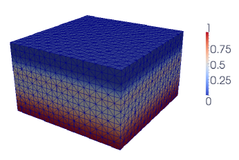
Figure 1. The mesh and surface plots of the amplitude of the associated solution for the scattered field $\boldsymbol{v}_{h}^{\rm PML}$ for Example 1: (left) the amplitude of the real part of the solution $|{\rm Re}\boldsymbol{v}_{h}^{\rm PML}|$; (right) the amplitude of the imaginary part of the solution $|{\rm Im}\boldsymbol{v}_{h}^{\rm PML}|$.

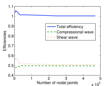
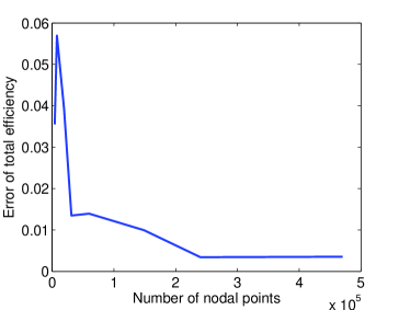
Figure 2. Grating efficiencies and robustness of grating efficiency for Example 1.

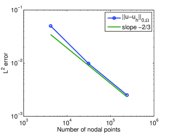
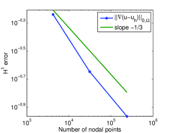
Figure 3. Quasi-optimality of $L^{2}$- and $H^{1}$- error estimates for Example 1.

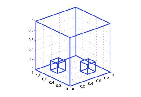
Figure 4. Geometry of the domain for Example 2.

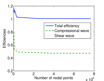
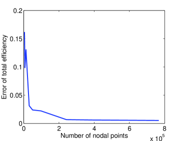
Figure 5. Grating efficiencies and robustness of grating efficiency for Example 2.

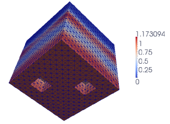
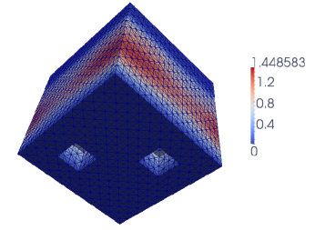
Figure 6. The mesh and surface plots of the amplitude of the associated solution for the scattered field $\boldsymbol{v}_{h}^{\rm PML}$ for Example 2: (left) the amplitude of the real part of the solution $|{\rm Re}\boldsymbol{v}_{h}^{\rm PML}|$; (right) the amplitude of the imaginary part of the solution $|{\rm Im}\boldsymbol{v}_{h}^{\rm PML}|$.

5. Concluding remarks

We have studied a variational formulation for the elastic wave scattering problem in a biperiodic structure and adopted the PML to truncate the physical domain. The scattering problem is reduced to a boundary value problem by using transparent boundary conditions. We prove that the truncated PML problem has a unique weak solution which converges exponentially to the solution of the original problem by increasing the PML paramers. Numerical results show that the proposed method is effective to solve the scattering problem of elastic waves in biperiodic structures. Although the paper presents the results for the rigid boundary condition, the method is applicable to other boundary conditions or the transmission problem where the structures are penetrable. This work considers only the uniform mesh refinement. We plan to incorporate the adaptive mesh refinement with a posteriori error estimate for the finite element method to handle the problems where the solutions may have singularities. The progress will be reported elsewhere in a future work.

Appendix A Technical estimates

In this section, we present the proofs for some technical estimates which are used in our analysis for the error estimate between the solutions of the PML problem and the original scattering problem.

Proposition A.1.

For any $n\in\mathbb{Z}^{2}$, we have $\kappa_{1}^{2}<|\chi^{(n)}|<\kappa_{2}^{2}$.

Proof.

Recalling (2.13) and (2.8), we consider three cases:

1. For $n\in U_{1}$, $\beta_{1}^{(n)}=(\kappa_{1}^{2}-|\boldsymbol{\alpha}^{(n)}|^{2})^{1/2}$ and $\beta_{2}^{(n)}=(\kappa_{2}^{2}-|\boldsymbol{\alpha}^{(n)}|^{2})^{1/2}$. We have

   $$\chi^{(n)}=|\boldsymbol{\alpha}^{(n)}|^{2}+\beta_{1}^{(n)}\beta_{2}^{(n)}=|\boldsymbol{\alpha}^{(n)}|^{2}+(\kappa_{1}^{2}-|\boldsymbol{\alpha}^{(n)}|^{2})^{1/2}(\kappa_{2}^{2}-|\boldsymbol{\alpha}^{(n)}|^{2})^{1/2}.$$

   Consider the function

   $$g_{1}(t)=t+(k_{1}-t)^{1/2}(k_{2}-t)^{1/2},\quad 0<k_{1}<k_{2}.$$

   It is easy to know that $g_{1}$ is decreasing for $0<t<k_{1}$. Hence

   $$k_{1}=g_{1}(k_{1})<g_{1}(t)<g_{1}(0)=(k_{1}k_{2})^{1/2},$$

   which gives $\kappa_{1}^{2}<\chi^{(n)}<\kappa_{1}\kappa_{2}$.

2. For $n\in U_{2}\setminus U_{1}$, $\beta_{1}^{(n)}={\rm i}(|\boldsymbol{\alpha}^{(n)}|^{2}-\kappa_{1}^{2})^{1/2},\beta_{2}^{(n)}=(\kappa_{2}^{2}-|\boldsymbol{\alpha}^{(n)}|^{2})^{1/2}$. We have

   $$\chi^{(n)}=|\boldsymbol{\alpha}^{(n)}|^{2}+{\rm i}(|\boldsymbol{\alpha}^{(n)}|^{2}-\kappa_{1}^{2})^{1/2}(\kappa_{2}^{2}-|\boldsymbol{\alpha}^{(n)}|^{2})^{1/2}$$

   and

   $$|\chi^{(n)}|^{2}=(\kappa_{1}^{2}+\kappa_{2}^{2})|\boldsymbol{\alpha}^{(n)}|^{2}-(\kappa_{1}\kappa_{2})^{2},$$

   which gives $\kappa_{1}^{2}<|\chi^{(n)}|<\kappa_{2}^{2}$.

3. For $n\notin U_{2}$, $\beta_{1}^{(n)}={\rm i}(|\boldsymbol{\alpha}^{(n)}|^{2}-\kappa_{1}^{2})^{1/2},\beta_{2}^{(n)}={\rm i}(|\boldsymbol{\alpha}^{(n)}|^{2}-\kappa_{2}^{2})^{1/2}$. We have

   $$\chi^{(n)}=|\boldsymbol{\alpha}^{(n)}|^{2}-(|\boldsymbol{\alpha}^{(n)}|^{2}-\kappa_{1}^{2})^{1/2}(|\boldsymbol{\alpha}^{(n)}|^{2}-\kappa_{2}^{2})^{1/2}.$$

   Let

   $$g_{2}(t)=t-(t-k_{1})^{1/2}(t-k_{2})^{1/2},\quad 0<k_{1}<k_{2}.$$

   It is easy to verify that the function $g_{2}$ is decreasing for $t>k_{2}$. Hence we have

   $$(k_{1}+k_{2})/2=g_{2}(\infty)<g_{2}(t)<g_{2}(k_{2})=k_{2},$$

   which gives $(\kappa_{1}^{2}+\kappa_{2}^{2})/2<\chi^{(n)}<\kappa_{2}^{2}$.

Combining the above estimates, we get $\kappa_{1}^{2}<|\chi^{(n)}|<\kappa_{2}^{2}$ for any $n\in\mathbb{Z}^{2}$. ∎

Proposition A.2.

The function $g_{3}(t)=t^{k}/e^{(t^{2}-s^{2})^{1/2}}$ satisfies $g_{5}(t)\leq(s^{2}+k^{2})^{k/2}$ for any $t>s>0,~{}k\in\mathbb{R}^{1}$.

Proof.

Using the change of variables $\tau=(t^{2}-s^{2})^{1/2}$, we have

$$\hat{g}_{3}(\tau)=\frac{(\tau^{2}+s^{2})^{k/2}}{e^{\tau}}.$$

Taking the derivative of $\hat{g}_{4}$ gives

$$\hat{g}^{\prime}_{3}(\tau)=-\frac{(\tau^{2}-k\tau+s^{2})(\tau^{2}+s^{2})^{\frac{k}{2}-1}}{e^{\tau}}.$$

1. If $s\geq k/2$, then $\hat{g}_{3}^{\prime}\leq 0$ for $\tau>0$. The function $\hat{g}_{3}$ is decreasing and reaches its maximum at $\tau=0$, i.e.,

   $$g_{3}(t)\leq\hat{g}_{3}(0)=s^{k}.$$

2. If $s<k/2$, then $\hat{g}^{\prime}_{3}<0$ for $\tau\in(0,(k-(k^{2}-4s^{2})^{1/2})/2)\cup((k+(k^{2}-4s^{2})^{1/2})/2,\infty)$ and $\hat{g}_{3}>0$ for $\tau\in((k-(k^{2}-4s^{2})^{1/2})/2,(k+(k^{2}-4s^{2})^{1/2})/2)$. Thus $\hat{g}_{3}$ reaches its maximum at either $\tau_{1}=0$ or $\tau_{2}=(k+(k^{2}-4s^{2})^{1/2})/2$. Thus we have

   $$g_{3}(t)=\hat{g}_{3}(\tau)\leq\max\{\hat{g}_{3}(\tau_{1}),\,\hat{g}_{3}(\tau_{2})\}\leq(s^{2}+k^{2})^{k/2}.$$

The proof is completed by combining the above estimates. ∎

Proposition A.3.

For any $n\in\mathbb{Z}^{2}$, we have $\|M^{(n)}-\hat{M}^{(n)}\|_{F}\leq\hat{K}$, where $\hat{K}=11\mu K/\kappa_{1}^{4}$.

Proof.

We consider the three cases:

1. For $n\in U_{1}$, we have $|\boldsymbol{\alpha}^{(n)}|<\kappa_{1},\beta_{1}^{(n)}=\Delta_{1}^{(n)}<\kappa_{1},\beta_{2}^{(n)}=\Delta_{2}^{(n)}<\kappa_{2}$, and $\Delta_{1}^{(n)}<\Delta_{2}^{(n)}$. Using the facts that $\kappa_{1}<\kappa_{2}$, $\Delta_{i}^{(n)}\geq{\Delta}^{-}_{\,i}$ for $n\in U_{1}$, we obtain from (2.13) and Proposition A.1 and A.2 that

   $$|\varepsilon^{(n)}|\leq\frac{2e^{-\Delta_{2}^{(n)}{\rm Im}\zeta}}{e^{\Delta_{2}^{(n)}{\rm Im}\zeta}-e^{-\Delta_{2}^{(n)}{\rm Im}\zeta}}\leq\frac{2}{e^{2\Delta_{2}^{(n)}{\rm Im}\zeta}-1}\leq\frac{2}{e^{\Delta_{1}^{(n)}{\rm Im}\zeta}-1}\leq\frac{2}{e^{{\Delta}^{-}_{\,1}{\rm Im}\zeta}-1},$$

   $$|\theta^{(n)}|\leq\frac{(e^{-\Delta_{2}^{(n)}{\rm Im}\zeta}+e^{-\Delta_{1}^{(n)}{\rm Im}\zeta})^{2}}{(1-e^{-2\Delta_{1}^{(n)}{\rm Im}\zeta})(1-e^{-2\Delta_{2}^{(n)}{\rm Im}\zeta})}\leq\frac{4e^{-2{\Delta}^{-}_{\,1}{\rm Im}\zeta}}{(1-e^{-2{\Delta}^{-}_{\,1}{\rm Im}\zeta})^{2}}\leq\frac{4}{(e^{\frac{1}{2}{\Delta}^{-}_{\,1}{\rm Im}\zeta}-1)^{2}},$$

   $$|\eta^{(n)}|\leq\frac{e^{-2\Delta_{2}^{(n)}{\rm Im}\zeta}+e^{-2\Delta_{1}^{(n)}{\rm Im}\zeta}}{(1-e^{-2\Delta_{1}^{(n)}{\rm Im}\zeta})(1-e^{-2\Delta_{2}^{(n)}{\rm Im}\zeta})}\leq\frac{2e^{-2{\Delta}^{-}_{\,1}{\rm Im}\zeta}}{(1-e^{-2{\Delta}^{-}_{\,1}{\rm Im}\zeta})^{2}}\leq\frac{2}{(e^{\frac{1}{2}{\Delta}^{-}_{\,1}{\rm Im}\zeta}-1)^{2}},$$

   $$|\gamma^{(n)}|\leq\frac{e^{-2\Delta_{1}^{(n)}{\rm Im}\zeta}+e^{-4\Delta_{2}^{(n)}{\rm Im}\zeta}}{(1-e^{-2\Delta_{1}^{(n)}{\rm Im}\zeta})(1-e^{-2\Delta_{2}^{(n)}{\rm Im}\zeta})^{2}}\leq\frac{2e^{-2\Delta_{1}^{(n)}{\rm Im}\zeta}}{(1-e^{-2\Delta_{1}^{(n)}{\rm Im}\zeta})^{3}}\leq\frac{2}{(e^{\frac{1}{3}{\Delta}^{-}_{\,1}{\rm Im}\zeta}-1)^{3}},$$

   $$|\theta^{(n)}(\varepsilon^{(n)}+1)|\leq \frac{4e^{-2\Delta_{1}^{(n)}{\rm Im}\zeta}}{(1-e^{-2\Delta_{1}^{(n)}{\rm Im}\zeta})^{2}}\frac{e^{\Delta_{2}^{(n)}{\rm Im}\zeta}+e^{-\Delta_{2}^{(n)}{\rm Im}\zeta}}{e^{\Delta_{2}^{(n)}{\rm Im}\zeta}-e^{-\Delta_{2}^{(n)}{\rm Im}\zeta}}$$

   $$\leq \frac{4e^{-2\Delta_{1}^{(n)}{\rm Im}\zeta}}{(1-e^{-2\Delta_{1}^{(n)}{\rm Im}\zeta})^{2}}\frac{2}{1-e^{-2\Delta_{1}^{(n)}{\rm Im}\zeta}}\leq\frac{8}{(e^{\frac{1}{3}{\Delta}^{-}_{\,1}{\rm Im}\zeta}-1)^{3}},$$

   $$|\hat{\chi}^{(n)}-\chi^{(n)}|\leq 4\kappa_{2}^{2}|\theta^{(n)}|\leq F,$$

   $$\max\Big{\{} |\big{(}(\alpha_{1}^{(n)})^{2}(\beta_{1}^{(n)}-\beta_{2}^{(n)})+\beta_{2}^{(n)}\chi^{(n)}\big{)}\chi^{(n)}\varepsilon^{(n)}|,|\alpha_{1}^{(n)}\alpha_{2}^{(n)}(\beta_{1}^{(n)}-\beta_{2}^{(n)})\chi^{(n)}\varepsilon^{(n)}|,$$

   $$|\big{(}(\alpha_{2}^{(n)})^{2}(\beta_{1}^{(n)}-\beta_{2}^{(n)})+\beta_{2}^{(n)}\chi^{(n)}\big{)}\chi^{(n)}\varepsilon^{(n)}|,|\beta_{2}^{(n)}\kappa_{2}^{2}\chi^{(n)}\varepsilon^{(n)}|\Big{\}}\leq 3\kappa_{2}^{5}|\varepsilon^{(n)}|\leq F,$$

   $$\max\Big{\{} |\big{(}(\alpha_{1}^{(n)})^{2}(\beta_{1}^{(n)}-\beta_{2}^{(n)})+\beta_{2}^{(n)}\chi^{(n)}\big{)}(\hat{\chi}^{(n)}-\chi^{(n)})|,|\alpha_{1}^{(n)}\alpha_{2}^{(n)}(\beta_{1}^{(n)}-\beta_{2}^{(n)})(\hat{\chi}^{(n)}-\chi^{(n)})|,$$

   $$|\big{(}(\alpha_{2}^{(n)})^{2}(\beta_{1}^{(n)}-\beta_{2}^{(n)})+\beta_{2}^{(n)}\chi^{(n)}\big{)}(\hat{\chi}^{(n)}-\chi^{(n)})|,|\alpha_{1}^{(n)}\beta_{2}^{(n)}(\beta_{1}^{(n)}-\beta_{2}^{(n)})(\hat{\chi}^{(n)}-\chi^{(n)})|,$$

   $$|\alpha_{2}^{(n)}\beta_{2}^{(n)}(\beta_{1}^{(n)}-\beta_{2}^{(n)})(\hat{\chi}^{(n)}-\chi^{(n)})|,|\beta_{2}^{(n)}\kappa_{2}^{2}(\hat{\chi}^{(n)}-\chi^{(n)})|\Big{\}}\leq 12\kappa_{2}^{5}|\theta^{(n)}|\leq F,$$

   $$\max\Big{\{} |4(\alpha_{2}^{(n)})^{2}\beta_{1}^{(n)}(\beta_{2}^{(n)})^{2}\theta^{(n)}(\varepsilon^{(n)}+1)|,|4\alpha_{1}^{(n)}\alpha_{2}^{(n)}\beta_{1}^{(n)}(\beta_{2}^{(n)})^{2}\theta^{(n)}(\varepsilon^{(n)}+1)|,$$

   $$|4(\alpha_{1}^{(n)})^{2}\beta_{1}^{(n)}(\beta_{2}^{(n)})^{2}\theta^{(n)}(\varepsilon^{(n)}+1)|\Big{\}}\leq 4\kappa_{2}^{5}|\theta^{(n)}(\varepsilon^{(n)}+1)|\leq F,$$

   $$\max\Big{\{} |2(\alpha_{1}^{(n)})^{2}\beta_{1}^{(n)}\kappa_{2}^{2}\eta^{(n)}|,|2\alpha_{1}^{(n)}\alpha_{2}^{(n)}\beta_{1}^{(n)}\chi^{(n)}\eta^{(n)}|,$$

   $$2(\alpha_{2}^{(n)})^{2}\beta_{1}^{(n)}\kappa_{2}^{2}\eta^{(n)}|,|2\beta_{1}^{(n)}(\beta_{2}^{(n)})^{2}\kappa_{2}^{2}\eta^{(n)}|\Big{\}}\leq 2\kappa_{2}^{5}|\eta^{(n)}|\leq F,$$

   $$|2\alpha_{1}^{(n)}\alpha_{1}^{(n)}\beta_{1}^{(n)}\beta_{2}^{(n)}(\beta_{1}^{(n)}-\beta_{2}^{(n)})\gamma^{(n)}|\leq 4\kappa_{2}^{5}|\gamma^{(n)}|\leq F,$$

   $$\max\Big{\{}|2\alpha_{1}^{(n)}\beta_{1}^{(n)}\beta_{2}^{(n)}(\kappa_{2}^{2}-2(\beta_{2}^{(n)})^{2})\theta^{(n)}|,|2\alpha_{2}^{(n)}\beta_{1}^{(n)}\beta_{2}^{(n)}(\kappa_{2}^{2}-2(\beta_{2}^{(n)})^{2})\theta^{(n)}|\Big{\}}\leq 6\kappa_{2}^{5}|\theta^{(n)}|\leq F,$$

2. For $n\in U_{2}\setminus U_{1}$, we have $|\boldsymbol{\alpha}^{(n)}|<\kappa_{2},\beta_{1}^{(n)}={\rm i}\Delta_{1}^{(n)},\beta_{2}^{(n)}=\Delta_{2}^{(n)}<\kappa_{2}$, $\Delta_{1}^{(n)}<(\kappa_{2}^{2}-\kappa_{1}^{2})^{1/2}<\kappa_{2}$. Using the facts that $\Delta_{1}^{(n)}\geq{\Delta}^{+}_{1},\Delta_{2}^{(n)}\geq{\Delta}^{-}_{\,2}$ for $n\in U_{2}\setminus U_{1}$, we get from Proposition A.1 and A.2 that

   $$|\varepsilon^{(n)}|=\frac{2e^{-\Delta_{2}^{(n)}{\rm Im}\zeta}}{e^{\Delta_{2}^{(n)}{\rm Im}\zeta}-e^{-\Delta_{2}^{(n)}{\rm Im}\zeta}}\leq\frac{2}{e^{2\Delta_{2}^{(n)}{\rm Im}\zeta}-1}\leq\frac{2}{e^{2{\Delta}^{-}_{\,2}{\rm Im}\zeta}-1}\leq\frac{2}{e^{{\Delta}^{-}_{\,2}{\rm Im}\zeta}-1},$$

   $$|\theta^{(n)}|\leq\frac{(e^{-\Delta_{2}^{(n)}{\rm Im}\zeta}+e^{-\Delta_{1}^{(n)}{\rm Re}\zeta})^{2}}{(1-e^{-2\Delta_{1}^{(n)}{\rm Re}\zeta})(1-e^{-2\Delta_{2,j}^{(n)}{\rm Im}\zeta})}\leq\frac{(e^{-{\Delta}^{-}_{\,2}{\rm Im}\zeta}+e^{-{\Delta}^{+}_{1}{\rm Re}\zeta})^{2}}{(1-e^{-2{\Delta}^{+}_{1}{\rm Re}\zeta})(1-e^{-2{\Delta}^{-}_{\,2}{\rm Im}\zeta})},$$

   $$|\eta^{(n)}|\leq \frac{e^{-2\Delta_{2}^{(n)}{\rm Im}\zeta}+e^{-2\Delta_{1}^{(n)}{\rm Re}\zeta}}{(1-e^{-2\Delta_{1}^{(n)}{\rm Re}\zeta})(1-e^{-2\Delta_{2}^{(n)}{\rm Im}\zeta})}\leq\frac{e^{-2{\Delta}^{-}_{2}{\rm Im}\zeta}+e^{-2{\Delta}^{+}_{1}{\rm Re}\zeta}}{(1-e^{-2{\Delta}^{+}_{1}{\rm Re}\zeta})(1-e^{-2{\Delta}^{-}_{2}{\rm Im}\zeta})}$$

   $$\leq \frac{(e^{-{\Delta}^{-}_{2}{\rm Im}\zeta}+e^{-{\Delta}^{+}_{1}{\rm Re}\zeta})^{2}}{(1-e^{-2{\Delta}^{+}_{1}{\rm Re}\zeta})(1-e^{-2{\Delta}^{-}_{2}{\rm Im}\zeta})},$$

   $$|\gamma^{(n)}|\leq \frac{e^{-2\Delta_{1}^{(n)}{\rm Re}\zeta}+e^{-4\Delta_{2}^{(n)}{\rm Im}\zeta}}{(1-e^{-2\Delta_{1}^{(n)}{\rm Re}\zeta})(1-e^{-2\Delta_{2}^{(n)}{\rm Im}\zeta})^{2}}\leq\frac{e^{-2{\Delta}^{+}_{1}{\rm Re}\zeta}+e^{-4{\Delta}^{-}_{\,2}{\rm Im}\zeta}}{(1-e^{-2{\Delta}^{+}_{1}{\rm Re}\zeta})(1-e^{-2{\Delta}^{-}_{\,2}{\rm Im}\zeta})^{2}}$$

   $$\leq \frac{(e^{-{\Delta}^{-}_{\,2}{\rm Im}\zeta}+e^{-{\Delta}^{+}_{1}{\rm Re}\zeta})^{2}}{(1-e^{-2{\Delta}^{+}_{1}{\rm Re}\zeta})(1-e^{-2{\Delta}^{-}_{2}{\rm Im}\zeta})},$$

   $$|\theta^{(n)}(\varepsilon^{(n)}+1)|\leq \frac{(e^{-\Delta_{2}^{(n)}{\rm Im}\zeta}+e^{-\Delta_{1}^{(n)}{\rm Re}\zeta})^{2}}{(1-e^{-2\Delta_{1}^{(n)}{\rm Re}\zeta})(1-e^{-2\Delta_{2}^{(n)}{\rm Im}\zeta})}\frac{2}{1-e^{-2\Delta_{2}^{(n)}{\rm Im}\zeta}}$$

   $$\leq \frac{2(e^{-{\Delta}^{-}_{2}{\rm Im}\zeta}+e^{-{\Delta}^{+}_{1}{\rm Re}\zeta})^{2}}{(1-e^{-2{\Delta}^{+}_{1}{\rm Re}\zeta})(1-e^{-2{\Delta}^{-}_{2}{\rm Im}\zeta})^{2}},$$

   $$|\hat{\chi}^{(n)}-\chi^{(n)}|\leq\frac{4\kappa_{2}^{4}}{\kappa_{1}^{2}}|\theta^{(n)}|\leq F,$$

   $$\max\Big{\{} |\big{(}(\alpha_{1}^{(n)})^{2}(\beta_{1}^{(n)}-\beta_{2}^{(n)})+\beta_{2}^{(n)}\chi^{(n)}\big{)}\chi^{(n)}\varepsilon^{(n)}|,|\alpha_{1}^{(n)}\alpha_{2}^{(n)}(\beta_{1}^{(n)}-\beta_{2}^{(n)})\chi^{(n)}\varepsilon^{(n)}|,$$

   $$|\big{(}(\alpha_{2}^{(n)})^{2}(\beta_{1}^{(n)}-\beta_{2}^{(n)})+\beta_{2}^{(n)}\chi^{(n)}\big{)}\chi^{(n)}\varepsilon^{(n)}|,|\beta_{2}^{(n)}\kappa_{2}^{2}\chi^{(n)}\varepsilon^{(n)}|\Big{\}}\leq 3\kappa_{2}^{5}|\varepsilon^{(n)}|\leq F,$$

   $$\max\Big{\{} |\big{(}(\alpha_{1}^{(n)})^{2}(\beta_{1}^{(n)}-\beta_{2}^{(n)})+\beta_{2}^{(n)}\chi^{(n)}\big{)}(\hat{\chi}^{(n)}-\chi^{(n)})|,|\alpha_{1}^{(n)}\alpha_{2}^{(n)}(\beta_{1}^{(n)}-\beta_{2,j}^{(n)})(\hat{\chi}^{(n)}-\chi^{(n)})|,$$

   $$|\big{(}(\alpha_{2}^{(n)})^{2}(\beta_{1}^{(n)}-\beta_{2}^{(n)})+\beta_{2}^{(n)}\chi^{(n)}\big{)}(\hat{\chi}^{(n)}-\chi^{(n)})|,|\alpha_{1}^{(n)}\beta_{2}^{(n)}(\beta_{1}^{(n)}-\beta_{2}^{(n)})(\hat{\chi}^{(n)}-\chi^{(n)})|,$$

   $$|\alpha_{2}^{(n)}\beta_{2}^{(n)}(\beta_{1}^{(n)}-\beta_{2}^{(n)})(\hat{\chi}^{(n)}-\chi^{(n)})|,|\beta_{2}^{(n)}\kappa_{2}^{2}(\hat{\chi}^{(n)}-\chi^{(n)})|\Big{\}}\leq\frac{12\kappa_{2}^{7}}{\kappa_{1}^{2}}|\theta^{(n)}|\leq F,$$

   $$\max\Big{\{} |4(\alpha_{2}^{(n)})^{2}\beta_{1}^{(n)}(\beta_{2}^{(n)})^{2}\theta^{(n)}(\varepsilon^{(n)}+1)|,|4\alpha_{1}^{(n)}\alpha_{2}^{(n)}\beta_{1}^{(n)}(\beta_{2}^{(n)})^{2}\theta^{(n)}(\varepsilon^{(n)}+1)|,$$

   $$|4(\alpha_{1}^{(n)})^{2}\beta_{1}^{(n)}(\beta_{2}^{(n)})^{2}\theta^{(n)}(\varepsilon^{(n)}+1)|\Big{\}}\leq 4\kappa_{2}^{5}|\theta^{(n)}(\varepsilon^{(n)}+1)|\leq F,$$

   $$\max\Big{\{} |2(\alpha_{1}^{(n)})^{2}\beta_{1}^{(n)}\kappa_{2}^{2}\eta^{(n)}|,|2\alpha_{1}^{(n)}\alpha_{2}^{(n)}\beta_{1}^{(n)}\chi^{(n)}\eta^{(n)}|,$$

   $$|2(\alpha_{2}^{(n)})^{2}\beta_{1}^{(n)}\kappa_{2}^{2}\eta^{(n)}|,|2\beta_{1}^{(n)}(\beta_{2}^{(n)})^{2}\kappa_{2}^{2}\eta^{(n)}|\Big{\}}\leq 2\kappa_{2}^{5}|\eta^{(n)}|\leq F,$$

   $$|2\alpha_{1}^{(n)}\alpha_{2}^{(n)}\beta_{1}^{(n)}\beta_{2}^{(n)}(\beta_{1}^{(n)}-\beta_{2}^{(n)})\gamma^{(n)}|\leq 4\kappa_{2}^{5}|\gamma^{(n)}|\leq F,$$

   $$\max\Big{\{} |2\alpha_{1}^{(n)}\beta_{1}^{(n)}\beta_{2}^{(n)}(\kappa_{2}^{2}-2(\beta_{2}^{(n)})^{2})\theta^{(n)}|,|2\alpha_{2}^{(n)}\beta_{1}^{(n)}\beta_{2}^{(n)}(\kappa_{2}^{2}-2(\beta_{2}^{(n)})^{2})\theta^{(n)}|\Big{\}}$$

   $$\leq 6\kappa_{2}^{5}|\theta^{(n)}|\leq F.$$

3. For $n\notin U_{2}$, we have $\kappa_{2}<|\boldsymbol{\alpha}^{(n)}|,\beta_{1}^{(n)}={\rm i}\Delta_{1}^{(n)},\beta_{2}^{(n)}={\rm i}\Delta_{2}^{(n)}$, and $\Delta_{2}^{(n)}<\Delta_{1}^{(n)}<|\boldsymbol{\alpha}^{(n)}|$. Noting ${\rm Re}\zeta\geq 1$, we obtain from Proposition A.2 that

   $$|\varepsilon^{(n)}|\leq\frac{2e^{-\Delta_{2}^{(n)}{\rm Re}\zeta}}{e^{\Delta_{2}^{(n)}{\rm Re}\zeta}-e^{-\Delta_{2}^{(n)}{\rm Re}\zeta}}\leq\frac{2}{e^{\Delta_{2}^{(n)}{\rm Re}\zeta}}\frac{1}{e^{\Delta_{2}^{(n)}{\rm Re}\zeta}-1}\leq\frac{2}{e^{(|\boldsymbol{\alpha}^{(n)}|^{2}-\kappa_{2}^{2})^{1/2}}}\frac{1}{e^{{\Delta}^{+}_{2}{\rm Re}\zeta}-1},$$

   $$|\theta^{(n)}|\leq \frac{(e^{-\Delta_{2}^{(n)}{\rm Re}\zeta}+e^{-\Delta_{1}^{(n)}{\rm Re}\zeta})^{2}}{(1-e^{-2\Delta_{1}^{(n)}{\rm Re}\zeta})(1-e^{-2\Delta_{2}^{(n)}{\rm Re}\zeta})}\leq\frac{4e^{-2\Delta_{2}^{(n)}{\rm Re}\zeta}}{(1-e^{-2\Delta_{2}^{(n)}{\rm Re}\zeta})^{2}}$$

   $$\leq \frac{4}{e^{\Delta_{2}^{(n)}{\rm Re}\zeta}}\frac{e^{-\Delta_{2}^{(n)}{\rm Re}\zeta}}{(1-e^{-2\Delta_{2}^{(n)}{\rm Re}\zeta})^{2}}\leq\frac{4}{e^{\Delta_{2}^{(n)}}}\frac{1}{(e^{\frac{1}{2}\Delta_{2}^{(n)}{\rm Re}\zeta}-1)^{2}}$$

   $$\leq \frac{4}{e^{(|\boldsymbol{\alpha}^{(n)}|^{2}-\kappa_{2}^{2})^{1/2}}}\frac{1}{(e^{\frac{1}{2}{\Delta}^{+}_{2}{\rm Re}\zeta}-1)^{2}},$$

   $$|\eta^{(n)}|\leq \frac{e^{-2\Delta_{2}^{(n)}{\rm Re}\zeta}+e^{-2\Delta_{1}^{(n)}{\rm Re}\zeta}}{(1-e^{-2\Delta_{1}^{(n)}{\rm Re}\zeta})(1-e^{-2\Delta_{2}^{(n)}{\rm Re}\zeta})}\leq\frac{2e^{-2\Delta_{2}^{(n)}{\rm Re}\zeta}}{(1-e^{-2\Delta_{2}^{(n)}{\rm Re}\zeta})^{2}}$$

   $$\leq \frac{2}{e^{\Delta_{2}^{(n)}{\rm Re}\zeta}}\frac{e^{-\Delta_{2}^{(n)}{\rm Re}\zeta}}{(1-e^{-2\Delta_{2}^{(n)}{\rm Re}\zeta})^{2}}\leq\frac{2}{e^{\Delta_{2}^{(n)}}}\frac{1}{(e^{\frac{1}{2}\Delta_{2}^{(n)}{\rm Re}\zeta}-1)^{2}}$$

   $$\leq \frac{2}{e^{(|\boldsymbol{\alpha}^{(n)}|^{2}-\kappa_{2}^{2})^{1/2}}}\frac{1}{(e^{\frac{1}{2}{\Delta}^{+}_{2}{\rm Re}\zeta}-1)^{2}},$$

   $$|\gamma^{(n)}|\leq \frac{e^{-2\Delta_{1}^{(n)}{\rm Re}\zeta}+e^{-4\Delta_{2}^{(n)}{\rm Re}\zeta}}{(1-e^{-2\Delta_{1}^{(n)}{\rm Re}\zeta})(1-e^{-2\Delta_{2}^{(n)}{\rm Re}\zeta})^{2}}\leq\frac{2e^{-2\Delta_{2}^{(n)}{\rm Re}\zeta}}{(1-e^{-2\Delta_{2}^{(n)}{\rm Re}\zeta})^{3}}$$

   $$\leq \frac{2}{e^{\Delta_{2}^{(n)}{\rm Re}\zeta}}\frac{e^{-\Delta_{2}^{(n)}{\rm Re}\zeta}}{(1-e^{-2\Delta_{2}^{(n)}{\rm Re}\zeta})^{3}}\leq\frac{2}{e^{\Delta_{2}^{(n)}}}\frac{1}{(e^{\frac{1}{3}\Delta_{2}^{(n)}{\rm Re}\zeta}-1)^{3}}$$

   $$\leq \frac{2}{e^{(|\boldsymbol{\alpha}^{(n)}|^{2}-\kappa_{2}^{2})^{1/2}}}\frac{1}{(e^{\frac{1}{3}{\Delta}^{+}_{2}{\rm Re}\zeta}-1)^{3}},$$

   $$|\theta^{(n)}(\varepsilon^{(n)}+1)|\leq \frac{4e^{-2\Delta_{2}^{(n)}{\rm Re}\zeta}}{(1-e^{-2\Delta_{2}^{(n)}{\rm Re}\zeta})^{2}}\frac{2}{1-e^{-2\Delta_{2}^{(n)}{\rm Re}\zeta}}\leq\frac{8}{e^{\Delta_{2}^{(n)}{\rm Re}\zeta}}\frac{e^{-\Delta_{2}^{(n)}{\rm Re}\zeta}}{(1-e^{-2\Delta_{2}^{(n)}{\rm Re}\zeta})^{3}}$$

   $$\leq \frac{8}{e^{\Delta_{2}^{(n)}}}\frac{1}{(e^{\frac{1}{3}\Delta_{2}^{(n)}{\rm Re}\zeta}-1)^{3}}\leq\frac{8}{e^{(|\boldsymbol{\alpha}^{(n)}|^{2}-\kappa_{2}^{2})^{1/2}}}\frac{1}{(e^{\frac{1}{3}{\Delta}^{+}_{2}{\rm Re}\zeta}-1)^{3}},$$

   $$|\hat{\chi}^{(n)}-\chi^{(n)}|\leq \frac{4|\boldsymbol{\alpha}^{(n)}|^{4}|\theta^{(n)}|}{\kappa_{1}^{2}}\leq\frac{16}{\kappa_{1}^{2}}\frac{|\boldsymbol{\alpha}^{(n)}|^{4}}{e^{(|\boldsymbol{\alpha}^{(n)}|^{2}-\kappa_{2}^{2})^{1/2}}}\frac{1}{(e^{\frac{1}{2}{\Delta}^{+}_{2}{\rm Re}\zeta}-1)^{2}}$$

   $$\leq \frac{16(\kappa_{2}^{2}+16)^{2}}{\kappa_{1}^{2}(e^{\frac{1}{2}{\Delta}^{+}_{2}{\rm Re}\zeta}-1)^{2}}\leq F,$$

   $$\max\Big{\{} |\big{(}(\alpha_{1}^{(n)})^{2}(\beta_{1}^{(n)}-\beta_{2}^{(n)})+\beta_{2}^{(n)}\chi^{(n)}\big{)}\chi^{(n)}\varepsilon^{(n)}|,|\alpha_{1}^{(n)}\alpha_{2}^{(n)}(\beta_{1}^{(n)}-\beta_{2}^{(n)})\chi^{(n)}\varepsilon^{(n)}|,$$

   $$|\big{(}(\alpha_{2}^{(n)})^{2}(\beta_{1}^{(n)}-\beta_{2}^{(n)})+\beta_{2}^{(n)}\chi^{(n)})\chi^{(n)}\varepsilon^{(n)}|,|\beta_{2}^{(n)}\kappa_{2}^{2}\chi^{(n)}\varepsilon^{(n)}|\Big{\}}$$

   $$\leq 3\kappa_{2}^{2}|\boldsymbol{\alpha}^{(n)}|^{3}|\varepsilon^{(n)}|\leq\frac{|\boldsymbol{\alpha}^{(n)}|^{3}}{e^{(|\boldsymbol{\alpha}^{(n)}|^{2}-\kappa_{2}^{2})^{1/2}}}\frac{6\kappa_{2}^{2}}{e^{{\Delta}^{+}_{2}{\rm Re}\zeta}-1}\leq\frac{6\kappa_{2}^{2}(\kappa_{2}^{2}+9)^{3/2}}{e^{{\Delta}^{+}_{2}{\rm Re}\zeta}-1}\leq F,$$

   $$\max\Big{\{} |\big{(}(\alpha_{1}^{(n)})^{2}(\beta_{1}^{(n)}-\beta_{2}^{(n)})+\beta_{2}^{(n)}\chi^{(n)}\big{)}(\hat{\chi}^{(n)}-\chi^{(n)})|,|\alpha_{1}^{(n)}\alpha_{2}^{(n)}(\beta_{1}^{(n)}-\beta_{2}^{(n)})(\hat{\chi}^{(n)}-\chi^{(n)})|,$$

   $$|\big{(}(\alpha_{2}^{(n)})^{2}(\beta_{1}^{(n)}-\beta_{2}^{(n)})+\beta_{2}^{(n)}\chi^{(n)})(\hat{\chi}^{(n)}-\chi^{(n)})|,|\alpha_{1}^{(n)}\beta_{2}^{(n)}(\beta_{1}^{(n)}-\beta_{2}^{(n)})(\hat{\chi}^{(n)}-\chi^{(n)})|,$$

   $$|\alpha_{2}^{(n)}\beta_{2}^{(n)}(\beta_{1}^{(n)}-\beta_{2}^{(n)})(\hat{\chi}^{(n)}-\chi^{(n)})|,|\beta_{2}^{(n)}\kappa_{2}^{2}(\hat{\chi}^{(n)}-\chi^{(n)})|\Big{\}}$$

   $$\leq\frac{12|\boldsymbol{\alpha}^{(n)}|^{7}|\theta^{(n)}|}{\kappa_{1}^{2}}\leq\frac{48}{\kappa_{1}^{2}}\frac{|\boldsymbol{\alpha}^{(n)}|^{7}}{e^{(|\boldsymbol{\alpha}^{(n)}|^{2}-\kappa_{2}^{2})^{1/2}}}\frac{1}{(e^{\frac{1}{2}{\Delta}^{+}_{2}{\rm Re}\zeta}-1)^{2}}$$

   $$\leq\frac{48(\kappa_{2}^{2}+49)^{7/2}}{\kappa_{1}^{2}(e^{\frac{1}{2}{\Delta}^{+}_{2}{\rm Re}\zeta}-1)^{2}}\leq F,$$

   $$\max\Big{\{} |4(\alpha_{2}^{(n)})^{2}\beta_{1}^{(n)}(\beta_{2}^{(n)})^{2}\theta^{(n)}(\varepsilon^{(n)}+1)|,|4\alpha_{1}^{(n)}\alpha_{2}^{(n)}\beta_{1}^{(n)}(\beta_{2}^{(n)})^{2}\theta^{(n)}(\varepsilon^{(n)}+1)|,$$

   $$|4(\alpha_{1}^{(n)})^{2}\beta_{1}^{(n)}(\beta_{2}^{(n)})^{2}\theta^{(n)}(\varepsilon^{(n)}+1)|\Big{\}}$$

   $$\leq 4|\boldsymbol{\alpha}^{(n)}|^{5}|\theta^{(n)}(\varepsilon^{(n)}+1)|\leq\frac{32|\boldsymbol{\alpha}^{(n)}|^{5}}{e^{(|\boldsymbol{\alpha}^{(n)}|^{2}-(\kappa_{2}^{2})^{1/2}}}\frac{1}{(e^{\frac{1}{3}{\Delta}^{+}_{2}{\rm Re}\zeta}-1)^{3}}\leq\frac{32(\kappa_{2}^{2}+25)^{5/2}}{(e^{\frac{1}{3}{\Delta}^{+}_{2}{\rm Re}\zeta}-1)^{3}}\leq F,$$

   $$\max\Big{\{} |2(\alpha_{1}^{(n)})^{2}\beta_{1}^{(n)}\kappa_{2}^{2}\eta^{(n)}|,|2\alpha_{1}^{(n)}\alpha_{2}^{(n)}\beta_{1}^{(n)}\chi^{(n)}\eta^{(n)}|,|2(\alpha_{2}^{(n)})^{2}\beta_{1}^{(n)}\kappa_{2}^{2}\eta^{(n)}|,|2\beta_{1}^{(n)}(\beta_{2}^{(n)})^{2}\kappa_{2}^{2}\eta^{(n)}|\Big{\}}$$

   $$\leq 2\kappa_{2}^{2}|\boldsymbol{\alpha}^{(n)}|^{3}|\eta^{(n)}|\leq 4\kappa_{2}^{2}\frac{|\boldsymbol{\alpha}^{(n)}|^{3}}{e^{(|\boldsymbol{\alpha}^{(n)}|^{2}-\kappa_{2}^{2})^{1/2}}}\frac{1}{(e^{\frac{1}{2}{\Delta}^{+}_{2}{\rm Re}\zeta}-1)^{2}}\leq\frac{4\kappa_{2}^{2}(\kappa_{2}^{2}+9)^{3/2}}{(e^{\frac{1}{2}{\Delta}^{+}_{2}{\rm Re}\zeta}-1)^{2}}\leq F,$$

   $$|2\alpha_{1}^{(n)}\alpha_{2}^{(n)}\beta_{1}^{(n)}\beta_{2}^{(n)}(\beta_{1}^{(n)}-\beta_{2}^{(n)})\gamma^{(n)}|\leq 4|\boldsymbol{\alpha}^{(n)}|^{5}|\gamma^{(n)}|$$

   $$\leq \frac{8|\boldsymbol{\alpha}^{(n)}|^{5}}{e^{(|\boldsymbol{\alpha}^{(n)}|^{2}-\kappa_{2}^{2})^{1/2}}}\frac{1}{(e^{\frac{1}{3}{\Delta}^{+}_{2}{\rm Re}\zeta}-1)^{3}}\leq\frac{8(\kappa_{2}^{2}+25)^{5/2}}{(e^{\frac{1}{3}{\Delta}^{+}_{2}{\rm Re}\zeta}-1)^{3}}\leq F,$$

   $$\max\Big{\{} |2\alpha_{1}^{(n)}\beta_{1}^{(n)}\beta_{2}^{(n)}(\kappa_{2}^{2}-2(\beta_{2}^{(n)})^{2})\theta^{(n)}|,|2\alpha_{2}^{(n)}\beta_{1}^{(n)}\beta_{2}^{(n)}(\kappa_{2}^{2}-2(\beta_{2}^{(n)})^{2})\theta^{(n)}|\Big{\}}$$

   $$\leq 6|\boldsymbol{\alpha}^{(n)}|^{5}|\theta^{(n)}|\leq\frac{|\boldsymbol{\alpha}^{(n)}|^{5}}{e^{(|\boldsymbol{\alpha}^{(n)}|^{2}-\kappa_{2}^{2})^{1/2}}}\frac{24}{(e^{\frac{1}{2}{\Delta}^{+}_{2}{\rm Re}\zeta}-1)^{2}}\leq\frac{24((\kappa_{2})^{2}+25)^{\frac{5}{2}}}{(e^{\frac{1}{2}{\Delta}^{+}_{2}{\rm Re}\zeta}-1)^{2}}\leq F,$$

   where we have used the estimate for $g_{3}$ and the facts that $\Delta_{i}^{(n)}\geq\Delta_{i}^{+}$ for $n\notin U_{2}$.

It follows from Proposition A.1 and the estimate $|\hat{\chi}^{(n)}-\chi^{(n)}|\leq K$ that $\kappa_{1}^{2}-K\leq|\hat{\chi}^{(n)}|\leq\kappa_{2}^{2}+K$. Again, we may choose some proper PML parameters $\sigma$ and $\delta$ such that $K\leq\kappa_{1}^{2}/2$, which gives $|\hat{\chi}^{(n)}|\geq\kappa_{1}^{2}/2$. Using the matrix Frobenius norm and combining all the above estimates, we get

$$\| M^{(n)}-\hat{M}^{(n)}\|_{F}^{2}\leq\frac{4\mu^{2}}{\kappa_{1}^{8}}\Big{(}|\big{(}(\alpha_{1}^{(n)})^{2}(\beta_{1}^{(n)}-\beta_{2}^{(n)})+\beta_{2}^{(n)}\chi^{(n)}\big{)}\chi^{(n)}\varepsilon^{(n)}|^{2}+|2(\alpha_{1}^{(n)})^{2}\beta_{1}^{(n)}\kappa_{2}^{2}\eta^{(n)}|^{2}$$

$$+|\big{(}(\alpha_{1}^{(n)})^{2}(\beta_{1}^{(n)}-\beta_{2}^{(n)})+\beta_{2}^{(n)}\chi^{(n)}\big{)}(\hat{\chi}^{(n)}-\chi^{(n)})|^{2}+|4(\alpha_{2}^{(n)})^{2}\beta_{1}^{(n)}(\beta_{2}^{(n)})^{2}\theta^{(n)}(\varepsilon^{(n)}+1)|^{2}$$

$$+2|\alpha_{1}^{(n)}\alpha_{2}^{(n)}(\beta_{1}^{(n)}-\beta_{2}^{(n)})\chi^{(n)}\varepsilon^{(n)}|^{2}+2|\alpha_{1}^{(n)}\alpha_{2}^{(n)}(\beta_{1}^{(n)}-\beta_{2}^{(n)})(\hat{\chi}^{(n)}-\chi^{(n)})|^{2}$$

$$+2|2\alpha_{1}^{(n)}\alpha_{2}^{(n)}\beta_{1}^{(n)}\chi^{(n)}\eta^{(n)}|^{2}+2|4\alpha_{1}^{(n)}\alpha_{2}^{(n)}\beta_{1}^{(n)}(\beta_{2}^{(n)})^{2}\theta^{(n)}(\varepsilon^{(n)}+1)|^{2}+|2(\alpha_{2}^{(n)})^{2}\beta_{1}^{(n)}\kappa_{2}^{2}\eta^{(n)}|^{2}$$

$$+2|2\alpha_{1}^{(n)}\alpha_{2}^{(n)}\beta_{1}^{(n)}\beta_{2}^{(n)}(\beta_{1}^{(n)}-\beta_{2}^{(n)})\gamma^{(n)}|^{2}+2|\alpha_{1}^{(n)}\beta_{2}^{(n)}(\beta_{1}^{(n)}-\beta_{2}^{(n)})(\hat{\chi}^{(n)}-\chi^{(n)})|^{2}$$

$$+2|2\alpha_{1}^{(n)}\beta_{1}^{(n)}\beta_{2}^{(n)}(\kappa_{2}^{2}-2(\beta_{2}^{(n)})^{2})\theta^{(n)}|^{2}+|\big{(}(\alpha_{2}^{(n)})^{2}(\beta_{1}^{(n)}-\beta_{2}^{(n)})+\beta_{2}^{(n)}\chi^{(n)}\big{)}\chi^{(n)}\varepsilon^{(n)}|^{2}$$

$$+|\big{(}(\alpha_{2}^{(n)})^{2}(\beta_{1}^{(n)}-\beta_{2}^{(n)})+\beta_{2}^{(n)}\chi^{(n)}\big{)}(\hat{\chi}^{(n)}-\chi^{(n)})|^{2}+|4(\alpha_{1}^{(n)})^{2}\beta_{1}^{(n)}(\beta_{2}^{(n)})^{2}\theta^{(n)}(\varepsilon^{(n)}+1)|^{2}$$

$$+2|\alpha_{2}^{(n)}\beta_{2}^{(n)}(\beta_{1}^{(n)}-\beta_{2}^{(n)})(\hat{\chi}^{(n)}-\chi^{(n)})|^{2}+2|2\alpha_{2}^{(n)}\beta_{1}^{(n)}\beta_{2}^{(n)}(\kappa_{2}^{2}-2(\beta_{2}^{(n)})^{2})\theta^{(n)}|^{2}$$

$$+|\beta_{2}^{(n)}\kappa_{2}^{2}\chi^{(n)}\varepsilon^{(n)}|^{2}+|\beta_{2}^{(n)}\kappa_{2}^{2}(\hat{\chi}^{(n)}-\chi^{(n)})|^{2}+|2\beta_{1}^{(n)}(\beta_{2}^{(n)})^{2}\kappa_{2}^{2}\eta^{(n)}|^{2}\Big{)}\leq\frac{116\mu^{2}}{\kappa_{1}^{8}}K^{2},$$

which completes the proof. ∎

References

• [1] T. Arens, The scattering of plane elastic waves by a one-dimensional periodic surface, Math. Methods Appl. Sci., 22 (1999), 55–72.
• [2] T. Arens, A new integral equation formulation for the scattering of plane elastic waves by diffraction gratings, J. Integral Equations Applications, 11 (1999), 275–297.
• [3] I. Babuška and A. Aziz, Survey Lectures on Mathematical Foundations of the Finite Element Method, in The Mathematical Foundations of the Finite Element Method with Application to the Partial Differential Equations, ed. by A. Aziz, Academic Press, New York, 1973, 5–359.
• [4] G. Bao, Finite element approximation of time harmonic waves in periodic structures, SIAM J. Numer. Anal. , 32 (1995), 1155–1169.
• [5] G. Bao, Variational approximation of Maxwell’s equations in biperiodic structures, SIAM J. Appl. Math., 57 (1997), 364–381.
• [6] G. Bao, Z. Chen, and H. Wu, Adaptive finite element method for diffraction gratings, J. Opt. Soc. Amer. A, 22 (2005), 1106–1114.
• [7] G. Bao, D. C. Dobson, and J. A. Cox, Mathematical studies in rigorous grating theory, J. Opt. Soc. Amer. A, 12 (1995), 1029–1042.
• [8] G. Bao, L. Cowsar, and W. Masters, eds., Mathematical Modeling in Optical Science, Frontiers Appl. Math., 22, SIAM, Philadelphia, 2001.
• [9] G. Bao, P. Li, and H. Wu, An adaptive edge element method with perfectly matched absorbing layers for wave scattering by periodic structures, Math. Comp., 79 (2010), 1–34.
• [10] G. Bao and H. Wu, On the convergence of the solutions of PML equations for Maxwell’s equations, SIAM J. Numer. Anal., 43 (2005), 2121–2143.
• [11] J.-P. Bérenger, A perfectly matched layer for the absorption of electromagnetic waves, J. Comput. Phys., 114 (1994), 185–200.
• [12] J. H. Bramble and J. E. Pasciak, Analysis of a finite PML approximation for the three dimensional time-harmonic Maxwell and acoustic scattering problems, Math. Comp., 76 (2007), 597–614.
• [13] J. H. Bramble, J. E. Pasciak, and D. Trenev, Analysis of a finite PML approximation to the three dimensional elastic wave scattering problem, Math. Comp., 79 (2010), 2079–2101.
• [14] J. Chen and Z. Chen, An adaptive perfectly matched layer technique for 3-D time-harmonic electromagnetic scattering problems, Math. Comp., 77 (2008), 673–698.
• [15] X. Chen and A. Friedman, Maxwell’s equations in a periodic structure, Trans. Amer. Math. Soc., 323 (1991), 4650–507.
• [16] Z. Chen and H. Wu, An adaptive finite element method with perfectly matched absorbing layers for the wave scattering by periodic structures, SIAM J. Numer. Anal., 41 (2003), 799-826.
• [17] Z. Chen and X. Liu, An adptive perfectly matched layer technique for time-harmonic scattering problems, SIAM J. Numer. Anal., 43 (2005), 645–671.
• [18] Z. Chen, X. Xiang, and X. Zhang, Convergence of the PML method for elastic wave scattering problems, Math. Comp., to appear.
• [19] F. Collino and P. Monk, The perfectly matched layer in curvilinear coordinates, SIAM J. Sci. Comput., 19 (1998), 2061–1090.
• [20] F. Collino and C. Tsogka, Application of the perfectly matched absorbing layer model to the linear elastodynamic problem in anisotropic heterogeneous media, Geophysics, 66 (2001), 294–307.
• [21] W. Chew and W. Weedon, A 3D perfectly matched medium for modified Maxwell’s equations with stretched coordinates, Microwave Opt. Techno. Lett., 13 (1994), 599–604.
• [22] D. Dobson and A. Friedman, The time-harmonic Maxwell equations in a doubly periodic structure, J. Math. Anal. Appl., 166 (1992), 507–528.
• [23] J. Elschner and G. Hu, Variational approach to scattering of plane elastic waves by diffraction gratings, Math. Meth. Appl. Sci., 33 (2010), 1924–1941.
• [24] J. Elschner and G. Hu, Scattering of plane elastic waves by three-dimensional diffraction gratings, Math. Models Methods Appl. Sci., 22 (2012), 1150019.
• [25] F. D. Hastings, J. B. Schneider, and S. L. Broschat, Application of the perfectly matched layer (PML) absorbing boundary condition to elastic wave propagation, J. Acoust. Soc. Am., 100 (1996), 3061–3069.
• [26] T. Hohage, F. Schmidt, and L. Zschiedrich, Solving time-harmonic scattering problems based on the pole condition. II: Convergence of the PML method, SIAM J. Math. Anal., 35 (2003), 547–560.
• [27] X. Jiang, P. Li, J. Lv, and W. Zheng, An adaptive finite element method for the elastic wave scattering problem in periodic structure, preprint.
• [28] M. Lassas and E. Somersalo, On the existence and convergence of the solution of PML equations, Computing, 60 (1998), 229–241.
• [29] P. Li, Y. Wang, and Y. Zhao, Inverse elastic surface scattering with near-field data, Inverse Problems, 31 (2015), 035009.
• [30] PHG (Parallel Hierarchical Grid), http://lsec.cc.ac.cn/phg/.
• [31] E. Turkel and A. Yefet, Absorbing PML boundary layers for wave-like equations, Appl. Numer. Math., 27 (1998), 533–557.
• [32] Z. Wang, G. Bao, J. Li, P. Li, and H. Wu, An adaptive finite element method for the diffraction grating problem with transparent boundary condition, SIAM J. Numer. Anal., 53 (2015), 1585–1607.