Accurate modeling of plasma acceleration with arbitrary order pseudo-spectral particle-in-cell methods

Abstract

Particle in Cell (PIC) simulations are a widely used tool for the investigation of both laser- and beam-driven plasma acceleration. It is a known issue that the beam quality can be artificially degraded by numerical Cherenkov radiation (NCR) resulting primarily from an incorrectly modeled dispersion relation. Pseudo-spectral solvers featuring infinite order stencils can strongly reduce NCR – or even suppress it – and are therefore well suited to correctly model the beam properties. For efficient parallelization of the PIC algorithm, however, localized solvers are inevitable. Arbitrary order pseudo-spectral methods provide this needed locality. Yet, these methods can again be prone to NCR. Here, we show that acceptably low solver orders are sufficient to correctly model the physics of interest, while allowing for parallel computation by domain decomposition.

Introduction

Plasma accelerators provide high accelerating gradients and promise very compact next-generation particle accelerators as drivers for brilliant light sources Maier et al. (2012); Huang, Ding, and Schroeder (2012) and high energy physics Schroeder et al. (2010). Using laser or beam drivers, the acceleration of electron beams by multiple GeV over few-cm distances has been demonstrated in experiments Leemans et al. (2006, 2014); Litos et al. (2014); Wang et al. (2013). The improvement of beam quality, especially in terms of energy spread, remains crucial for applications. Due to the non-linear nature of the beam-plasma interaction, Particle-in-Cell (PIC) simulations are a vital tool to model the beam injection and transport in the plasma. PIC algorithms self-consistently solve the interaction of spatially discretized electromagnetic fields with charged particles defined in a continuous phase space. However, these codes can suffer from numerical Cherenkov radiation (NCR) Godfrey (1974) that is caused primarily by incorrect modeling of the electromagnetic dispersion relation. Mitigation of this effect is crucial as it gives rise to an unphysical degradation of beam quality which leads to wrong predictions when using those results as input for studies on applications such as compact Free-Electron Lasers. For example, NCR has been found to artificially decrease the beam quality in terms of transverse beam emittance Lehe et al. (2013) for finite-difference time domain (FDTD) solvers, such as the commonly used Yee scheme. Efforts to circumvent this issue include the modification of the FDTD dispersion relation Lehe et al. (2013); Cowan et al. (2013) and digital filtering Greenwood et al. (2004); Vay et al. (2011). In contrast to FDTD solvers, pseudo-spectral solvers, which solve Maxwell’s equations in spectral space, strongly reduce NCR – and sometimes even suppress it.
In practice, PIC simulation can easily demand thousands of hours of computation time. Therefore, implementations that are efficient and scalable for parallel production are unavoidable. The parallelization of PIC codes is typically done by decomposing the simulation volume into domains which are evaluated by individual processes. For FDTD algorithms efficient scaling to several thousand parallel processes is possible. Pseudo-spectral solvers, however, act globally on the grid due to the needed Fourier transform, which limits efficient parallelization. An approach to overcome this limitation are arbitrary order pseudo-spectral solvers Vay and Arefiev (2016); Vincenti and Vay (2016); Li et al. (2017), which only locally affect the fields when solving Maxwell’s equations. On the downside, this — again — introduces spurious numerical dispersion and can make a simulation prone to NCR.
In the following, we investigate numerical Cherenkov radiation and its implications on the physics of a simulation for arbitrary order pseudo-spectral solvers using the spectral, quasi-cylindrical PIC algorithm implemented in the code Fbpic Lehe et al. (2016a); Lehe and Kirchen (2017).
The paper is structured as follows. We will first summarize the concept of pseudo-spectral solvers, with an emphasis on the arbitrary order Vay and Arefiev (2016) pseudo-spectral analytic time domain (PSATD) Haber et al. (1973), followed by a discussion of the main characteristics of NCR. In the last part we numerically analyze the mitigation of NCR in the arbitrary order PSATD scheme. As a figure of merit for the physical accuracy of the solver we use the effect of NCR on the beam emittance and the slice energy spread. With parameter scans we show the dependence of NCR on physical and numerical parameters of the simulation.

Finite order pseudo-spectral solvers

A widely used method in PIC codes are FDTD solvers. These algorithms use finite difference operators to approximate derivatives in time and space when numerically solving Maxwell’s equations, which introduces a spurious numerical dispersion. This approximation can be done with arbitrary precision by increasing the used stencil order, i.e., taking contributions from more surrounding grid nodes into account. Yet, this has the drawback of also increasing the computational demand of the calculation. Further, common FDTD algorithms represent the electromagnetic fields on a staggered grid, where the electric and magnetic fields are not defined at the same points in time and space. This is known to cause errors when modeling the direct interaction between an electron beam and a co-propagating laser Lehe et al. (2014).
The use of finite differences in space can be avoided by transforming Maxwell’s equations into spectral space. In that case the differential operator $\partial_{z}$ is given by a multiplication with $ik_{z}$, which numerically can be evaluated without approximations. The resulting solver class is referred to as pseudo-spectral time domain (PSTD) Liu (1997) and it describes the limit of an FDTD solver with an infinite stencil order Vincenti and Vay (2016). Yet, this solver still applies finite difference approximations in time and thereby, like FDTD solvers, its timestep is limited by a Courant condition. It is subject to spurious numerical dispersion, but unlike FDTD schemes the erroneous dispersion caused by the PSTD scheme results in modes traveling faster than the speed of light Vay, Haber, and Godfrey (2013).
Under the assumption of constant currents $\boldsymbol{J}$ over one timestep $\Delta t$, this constraint can be overcome by integrating Maxwell’s equations analytically in time. With a precise representation of derivatives in time and space, the resulting pseudo-spectral analytic time domain (PSATD) scheme is not subject to a Courant condition and is free of spurious numerical dispersion. Furthermore, it is currently the only solver that can be combined with the Galilean scheme Kirchen et al. (2016); Lehe et al. (2016b) that is intrinsically stable when modeling relativisticly drifting plasmas with uniform velocity.
The PSATD field propagation equations in Cartesian coordinates are

$$\boldsymbol{\tilde{E}}^{n+1} =C\boldsymbol{\tilde{E}}^{n}+iS\boldsymbol{\hat{k}}\times\boldsymbol{\tilde{B}}^{n}-\frac{S}{ck}\boldsymbol{\tilde{J}}^{n+1/2}$$ (1a)

$$+i\frac{\boldsymbol{\hat{k}}}{k}\left[\left(\frac{S}{ck\Delta t}-1\right)\tilde{\rho}^{n+1}+\left(C-\frac{S}{ck\Delta t}\right)\tilde{\rho}^{n}\right]$$

$$\boldsymbol{\tilde{B}}^{n+1} =C\boldsymbol{\tilde{B}}^{n}-iS\boldsymbol{\hat{k}}\times\boldsymbol{\tilde{E}}^{n}+i\frac{1-C}{ck}\boldsymbol{\hat{k}}\times\boldsymbol{\tilde{J}}^{n+1/2},$$ (1b)

where $\boldsymbol{k}$ is the wave vector of length $k\equiv\sqrt{k_{x}^{2}+k_{y}^{2}+k_{z}^{2}}$ with $\boldsymbol{\hat{k}}=\boldsymbol{k}/k$ and $\tilde{F}$ is the Fourier transform of a field $F$, with $E$ and $B$ the electric and magnetic field, and $\rho$ and $J$ the charge and current density. Further, $C=\cos(kc\Delta t)$ and $S=\sin(kc\Delta t$). With pseudo-spectral methods the fields are naturally centered in space and time, eliminating a source of interpolation errors due to the usual staggering of the electromagnetic fields in the popular Yee FDTD solver. The equations of the PSTD scheme can be retrieved from those of the PSATD scheme, by writing the PSATD equations in an equivalent staggered form Vay, Haber, and Godfrey (2013) and performing a first-order Taylor expansion in $\Delta t$.
In the following we will use the PSATD scheme in a quasi-cylindrical geometry as derived in Ref. Lehe et al. (2016a). In this geometry the fields are decomposed into azimuthal modes $m$, which can then be represented on separate 2D grids Lifschitz et al. (2009). In practice, as the contributions from most of the modes go to zero for near-symmetrical systems, only a few of these have to be taken into account. Consequently, this geometry allows to model near-symmetrical problems at a drastically reduced computational effort compared to full 3D simulations. In the quasi-cylindrical PSATD scheme the real-space components $F_{r}$, $F_{\theta}$ and $F_{z}$ of a field $\boldsymbol{F}$ are connected to their spectral components $\tilde{F}_{+,m}$, $\tilde{F}_{-,m}$ and $\tilde{F}_{z}$ by the combination of a Hankel transform (along $r$) and a Fourier transform (along $z$). The equations of the quasi-cylindrical PSATD can be derived from the Cartesian PSATD scheme by replacing the differential operators in Eqs. (1a) and (1b) by Lehe et al. (2016b)

$$\boldsymbol{\tilde{F}}=i\boldsymbol{k}\tilde{S} \to\begin{pmatrix}\tilde{F}_{+,m}\\ \tilde{F}_{-,m}\\ \tilde{F}_{z,m}\end{pmatrix}=\begin{pmatrix}-k_{\perp}\tilde{S}_{m}/2\\ k_{\perp}\tilde{S}_{m}/2\\ ik_{z}\tilde{S}_{m}\end{pmatrix}$$ (2a)

$$\boldsymbol{\tilde{F}}=i\boldsymbol{k}\times\boldsymbol{\tilde{V}} \to\begin{pmatrix}\tilde{F}_{+,m}\\ \tilde{F}_{-,m}\\ \tilde{F}_{z,m}\end{pmatrix}=\begin{pmatrix}k_{z}\tilde{V}_{+,m}-ik_{\perp}\tilde{V}_{z,m}/2\\ -k_{z}\tilde{V}_{-,m}-ik_{\perp}\tilde{V}_{z,m}/2\\ ik_{\perp}\tilde{V}_{+,m}+ik_{\perp}\tilde{V}_{-,m},\end{pmatrix}$$ (2b)

where $\tilde{S}$ is any scalar field and $\boldsymbol{\tilde{V}}$ any vector field. This representation of the PSATD scheme preserves the advantages of the Cartesian PSATD scheme, i.e. an ideal dispersion relation, a centered representation of the fields and no Courant condition for the timestep, and combines them with the reduced computational demand associated with a quasi-cylindrical geometry.
The propagation of the fields in spectral space in Eqs. (1a) and (1b) corresponds to a global operation in spatial space, where information is transferred over the entire simulation grid. However, for domain decomposition a locality of the solver operations is necessary. In order to achieve an arbitrary order local stencil the solver equations are modified.
The formulations of the modified pseudo-spectral scheme can be derived from the expression of a finite difference with arbitrary order. For a centered scheme the discrete derivative with stencil order $2\,n$ of a function $F$ at a discrete point $p$ on the spatial grid is Fornberg (1988)

$$(D_{z}F)_{p} =\sum_{j=1}^{n}\alpha_{n,j}\frac{F_{p+j}-F_{p-j}}{2\,j\,\Delta z}$$ (3)

$$\alpha_{n,j} =(-1)^{j+1}\frac{2\,(n!)^{2}}{(n-j)!\;(n+j)!}.$$

To get a spectral method with a finite stencil derivative consider the spectral representation of this operator

$$(D_{z}F)_{p}=\sum_{k_{z}}i[k_{z}]\tilde{F}_{k_{z}}e^{ik_{z}p\Delta z}.$$ (4)

Here $[k_{z}]$ is the modified wavenumber given as

$$[k_{z}]=\sum_{j=1}^{n}\alpha_{n,j}\frac{\sin(k_{z}j\Delta z)}{j\,\Delta z},$$ (5)

with the grid spacing $\Delta z$ and $\tilde{F}$ the spectral form of $F$. This means that the equivalent to a finite stencil in real space can be achieved by using a modified PSTD algorithm, whereby $k_{z}$, $k_{x}$, $k_{y}$ are replaced by $[k_{z}]$, $[k_{x}]$, $[k_{y}]$ in the discretized Maxwell equations in spectral space. Because this modified PSTD algorithm is mathematically equivalent to an FDTD scheme (with high-order spatial derivatives), it has the same locality.
Similarly to the PSTD algorithm, in order to obtain a PSATD scheme with improved locality, we follow identical steps. More precisely, the discretized Maxwell equations Eqs. (1a) and (1b) are modified by replacing $k_{z}$, $k_{x}$, $k_{y}$ by $[k_{z}]$, $[k_{x}]$, $[k_{y}]$ – including in the expression of $k\equiv\sqrt{k_{x}^{2}+k_{y}^{2}+k_{z}^{2}}$ which in turn impacts the expressions of the coefficients $C$ and $S$. Consequently, unlike the modified PSTD algorithm, the modified PSATD scheme is not strictly local. In order to evaluate its locality, we get the corresponding stencil coefficients on the spatial grid, by applying an inverse Fourier transform to the operators used to advance the fields in Eqs. (1a) and (1b), i.e. $\boldsymbol{\hat{[k]}}S$ and $C$.

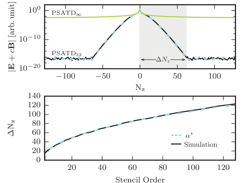
Figure 1: Expansion of an electromagnetic unit pulse after one PIC cycle with modified $k_{z}$ (top). The field pushed with the unmodified PSATD method (green line) shows non-negligible field contributions along the entire simulation grid, while the fields modeled with order 32 PSATD (black line) decrease by $16$ orders of magnitude over $\Delta N_{z}$ cells and reach the machine precision level. The number of cells over which the fields decrease (bottom) depends on the stencil order. The dashed lines show the stencil coefficients derived from the modified PSATD equations.

Next, we will use this scheme in quasi-cylindrical geometry with the PIC framework Fbpic to verify the locality of the solver. In Fbpic only $k_{z}$ is modified, because the Fourier transform is only used along the $z$-axis. Therefore, the corresponding solver stencil remains infinite in radial direction and locality is only gained in longitudinal direction. To examine this, a $\delta$-peak in E and B is initialized on axis in the center of the simulation box with a grid resolution of $\Delta r=\Delta z=1\,\upmu\mathrm{m}$. It is then propagated for one timestep $\Delta t=\Delta z/c$. Fig. 1 (top) shows the expansion of the pulse for a stencil order of 32 compared to the standard PSATD. When using the unmodified PSATD ($\text{PSATD}_{\infty}$) scheme the simulation shows field contributions along the entire axis, whereas the fields modeled with finite order PSATD quickly decrease in amplitude and reach the machine precision level. The expansion of the unit pulse strictly follows the stencil coefficients $\alpha*$ derived from the modified PSATD operations given by

$$\alpha^{*}=\sqrt{|\mathcal{F}^{-1}(C)^{2}|+|\mathcal{F}^{-1}(Sk_{\perp})^{2}|+|\mathcal{F}^{-1}(S[k_{z}])^{2}|},$$ (6)

where $\mathcal{F}^{-1}$ denotes an inverse Fourier transform along the $z$-axis. Here these coefficients are calculated numerically and instead of an analytical Fourier transform an FFT was used. The coefficients are evaluated for $k_{\perp}=0.5\,\upmu\mathrm{m}^{-1}$. The stencil coefficients as well as the unit pulse reach machine precision related noise after decreasing by $16$ orders of magnitude over a range of $\Delta N_{z}$ cells. In order to show how the stencil extent $\Delta N_{z}$ scales with the arbitrary order PSATD, the same simulation is done with varied stencil order. Fig. 1 (bottom) shows that the stencil extent behaves non-linearly to the applied stencil order. While for high orders the extent is similar to the stencil order, the reach of the solver tends to be bigger than the order in low order cases.
In a domain decomposition scheme the fields would only need to be exchanged between neighboring processes in guard regions with the size of $\Delta N_{z}$ cells, as this is the maximum distance information can travel within one timestep. These guard cells hold copies of the fields in the neighboring domains. At each timestep the fields are evaluated independently in each domain and the information is only exchanged in these cells. When significantly less than $\Delta N_{z}$ guard cells are used, truncation of the stencil can lead to spurious fields Vincenti and Vay (2016).
Note that for parallelization also a localized current correction or a charge conserving current deposition is needed. For that an exact current deposition in k-space for Cartesian coordinates Vay, Haber, and Godfrey (2013) and a local FFT based current correction on staggered grids Li et al. (2017) have been shown.
To summarize, in high order FDTD schemes the computational demand scales with the stencil order as an extension of the stencil to more neighboring cells calls for more individual numerical operations. In contrast, the stencil in spatial space for the arbitrary order PSATD is merely determined by the modification of the $k$ values in spectral space. Apart from this the scheme is identical to the infinite order PSATD. Therefore, the computational demand of the solver is independent of the stencil order and consequently also of the precision of the field solver. However, the improved locality of this schemes comes along with approximations on the integration of the electromagnetic fields which also result in spurious numerical dispersion. The implications of this will be discussed in the following.

Numerical Cherenkov radiation

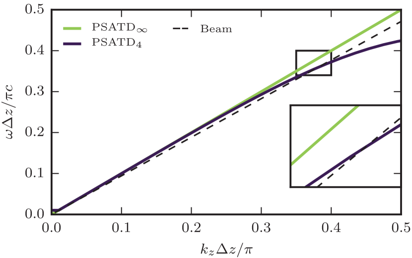
Figure 2: Dispersion relation for the arbitrary order PSATD solver (solid lines) on the $k_{z}$-Axis ($k_{r}=0$). Finite stencils introduce a spurious dispersion relation, which leads to a reduced phase velocity $v_{\phi,z}=\omega/k_{z}$ of modes with large $k_{z}$ and allows unphysical intersections (box) with the mode corresponding to the velocity of a relativistic particle (dashed line), here $\gamma_{\text{beam}}=3$. Particle beams can then travel with the same velocity as electromagnetic modes, which leads to coherent emission of spurious radiation, referred to as NCR.

In general, the phase velocity $v_{\phi}$ of an electromagnetic mode with wave vector $\boldsymbol{k}$ and angular frequency $\omega$ is $v_{\phi}^{2}=\omega^{2}/\boldsymbol{k}^{2}$. The allowed electromagnetic modes in vacuum are described by the dispersion relation

$$\omega^{2}=c^{2}\boldsymbol{k}^{2}.$$ (7)

When modifying $\boldsymbol{k}$ in longitudinal direction the dispersion relation is

$$\omega^{2}=c^{2}\left(k_{r}^{2}+[k_{z}]^{2}\right).$$ (8)

Here, a spurious numerical dispersion is introduced, where the phase velocity in vacuum decreases for modes with increasing $k_{z}$. Fig. 2 shows the distorted dispersion relation caused by the arbitrary order PSATD solver compared to the accurate case (Eq. (7)) given by the unmodified, infinite order PSATD method. Due to the distortion of the dispersion relation, relativistic particles can travel with the same velocity as some electromagnetic modes. This can lead to coherent emission of spurious radiation referred to as numerical Cherenkov radiation. Consequently, the affected modes obey

$$v_{\phi,z}=v_{\text{beam}},$$ (9)

where $v_{\text{beam}}$ is the velocity of the charged particles in the simulation. Using Eq. (8) this can be rewritten as

$$v_{\text{beam}}=\frac{c\sqrt{k_{r}^{2}+[k_{z}]^{2}}}{k_{z}}.$$ (10)

This condition describes the modes, where the spurious electromagnetic dispersion relation intersects with the beam mode corresponding to the velocity of a charged particle. This effect is illustrated in Fig. 3. The dashed lines indicate the modes fulfilling Eq. (10) and thus correspond to the intersection points of the dispersion relation and the beam mode as depicted in Fig. 2. These intersection points denote the modes where NCR is excited. They are overlaid with the spatial Fourier transform of the longitudinal electric field from Fbpic simulations, with parameters as discussed in the next section. The panels of Fig. 3 show results from simulations done with different stencil orders. They all show excited modes that can be attributed to the physics in the simulation of a beam driven plasma accelerator, e.g. the plasma wave or betatron radiation. However, compared to the unmodified $\mathrm{PSATD_{\infty}}$ scheme simulation, additional excited modes are visible around the modes prone to NCR. The excitations are especially strong for low solver orders. They decrease for higher stencil orders as the resonant modes of Eq. (10) move away from modes that can be attributed to the physics of the simulation. Eventually, for the $\mathrm{PSATD_{\infty}}$ the phase velocity $v_{\phi}$ is always greater than $v_{\mathrm{beam}}$ (i.e. no dashed line) and no NCR is present.
The analysis of the Fourier transformed electric field consequently can be used as an indication for the presence and magnitude of NCR. Next, we will show the influence of these unphysical modes on the properties of an electron beam.

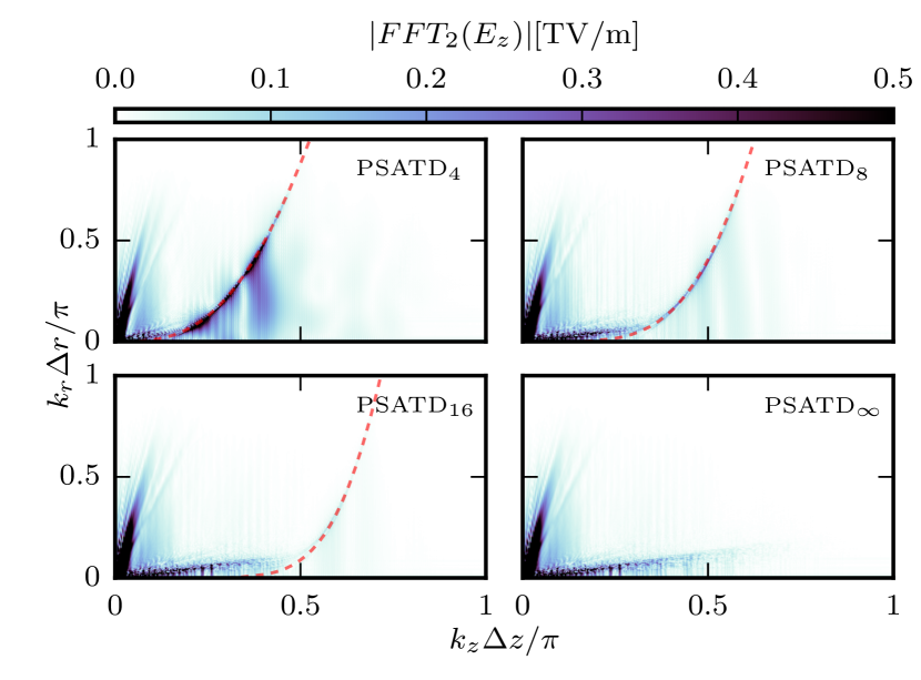
Figure 3: Spatial Fourier transforms of the accelerating field for simulations with different PSATD stencil orders. The simulations with finite order show resonances around the modes with a phase velocity matching the velocity of the electron beam (dashed lines) given by Eq. (10). The magnitude of NCR decreases for increasing stencil order. The NCR-free infinite order PSATD simulation is shown for reference.

Accurate modeling of plasma accelerators in finite order PSATD

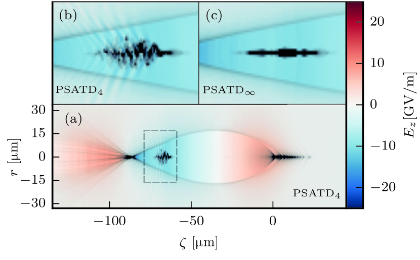
Figure 4: (a) Simulation setup featuring a driver and witness beam after propagating $35\,\mathrm{mm}$. Colors correspond to the accelerating field and the charge density is given in gray (arb. units), $\zeta=z-ct$ are the co-moving coordinates with $\zeta=0$ at the center of the driver beam. The short $\mathrm{PSATD_{4}}$ stencil leads to distortions of the longitudinal field around the witness beam (b) that are not present for an infinite order stencil (c).

To show that already low stencil orders are sufficient to mitigate errors due to NCR in the context of plasma-based acceleration, PIC simulations with the spectral, quasi-cylindrical code Fbpic for beam-driven plasma accelerator parameters are presented. Typical setups Grebenyuk et al. (2014); Litos et al. (2014) feature high bunch charges and consequently high currents, as they aim for applications in future brilliant light sources and high energy physics.
The propagation of cold, i.e. zero emittance, monoenergetic driver and witness electron beams through a plasma of density $1\times 10^{17}\;\mathrm{cm^{-3}}$ is simulated. A non-linear wakefield is driven by a 1 GeV Gaussian beam with a charge of 180 pC, $8.4\;\mathrm{\upmu m}$ rms length and $5\;\mathrm{\upmu m}$ rms width, compare Fig. 4(a). The 25 MeV Gaussian witness bunch of 50 pC charge, $2\;\mathrm{\upmu m}$ rms length and $1\;\mathrm{\upmu m}$ rms width is positioned in the accelerating region at the back of the bubble.
The simulation box has a resolution of 5 cells/$\mathrm{\upmu m}$ longitudinally and 1.5 cells/$\mathrm{\upmu m}$ transversally, with 16 particles per cell distributed as $2\times 2\times 4$ in longitudinal, radial and azimuthal direction, respectively. A total of 900 $\times$ 300 cells in two azimuthal modes is used. While the pseudo-spectral solver of Fbpic is technically not limited by a CFL condition, a timestep of $\Delta t=\Delta z/c$ was used. For the same physical parameters, the stencil order of the arbitrary order PSATD is varied. The NCR-free simulation with an infinite order stencil is used as a reference in the following.
Fig. 4 and 5 both show simulation results after a propagation through 35 mm of plasma. In Fig. 4 (b) and (c) the accelerating field $E_{z}$ and the charge density $\rho$ in the vicinity of the witness bunch can be seen. In the case of a low stencil order strong distortions are visible in $E_{z}$. The distortions are the spatial space equivalent to resonances visible for the $\mathrm{PSATD_{4}}$ in Fig. 3. These spurious fields affect the witness beam shape which corresponds to an increase of beam emittance, as it has been reported for 3D FDTD codes Lehe et al. (2013).
We find that also the longitudinal phase space is affected, as shown in Fig. 5, which compares the phase spaces modeled with several stencil orders. The projected energy spread increases during propagation through the plasma due to the slope of $E_{z}$ in combination with beam loading, so that an s-shape like structure is imprinted on the phase space also with $\mathrm{PSATD_{\infty}}$. However, for decreasing stencil order, NCR causes an increasingly violent high frequency oscillation on the longitudinal phase space, leading to an unphysical growth of both slice and projected energy spread. It can be observed that the perturbation is especially pronounced behind the beam center, where the current density is highest, while the head remains mostly unaffected.
Fig. 6 (top) shows the evolution of the slice energy spread during the propagation through the plasma for different solver orders. For finite order stencils the energy spread grows non-linearly with $z$. While $\mathrm{PSATD_{4}}$ and $\mathrm{PSATD_{8}}$ still deviate significantly from the Cherenkov free infinite order case, the impact of NCR on the beam in the PSATD₁₆ simulation is barely visible even after a long propagation distance. The dashed lines correspond to simulations done with the FDTD Yee scheme in 3D Cartesian and quasi-cylindrical geometry. These are performed with the PIC code Warp Vay et al. (2012) using the same parameters and resolution as Fbpic. With the Yee scheme the growth rate of spurious slice energy spread is even greater than for the low order PSATD case. Note that the Warp framework also features a $\mathrm{PSATD_{\infty}}$ (and arbitrary order) solver, which, if used for this problem, would also produce the correct physical results as the Fbpic $\mathrm{PSATD_{\infty}}$ algorithm.
Fig. 6 (bottom) shows the error of the slice energy spread and the transverse beam emittance and the longitudinal electric field after a propagation length of 35 mm depending on the stencil order. Here, the errors are defined as

$$\mathrm{Err}_{\sigma\gamma}=\sqrt{\frac{1}{N_{\mathrm{slice}}}\sum_{i}^{N_{\mathrm{slice}}}\left(\frac{\sigma_{\gamma,f,i}-\sigma_{\gamma,\infty,i}}{\sigma_{\gamma,\infty,i}}\right)^{2}},$$ (11)

$$\mathrm{Err}_{\epsilon}=\frac{\epsilon_{f}-\epsilon_{\infty}}{\epsilon_{\infty}},$$ (12)

$$\mathrm{Err}_{E_{z}}=\sqrt{\frac{1}{N_{z}N_{r}}\sum_{N_{z},N_{r}}\left(\frac{FFT_{2}(E_{z})_{f}-FFT_{2}(E_{z})_{\infty}}{FFT_{2}(E_{z})_{\infty}}\right)^{2}},$$ (13)

respectively. The subscripts $f$ and $\infty$ indicate quantities from finite and infinite order simulations. For the calculation of $\mathrm{Err}_{\sigma\gamma}$ $N_{\mathrm{slice}}$ slices of length $0.5$ $\upmu$m within $\pm 3\sigma_{z}$ of the witness beam are considered. For $\mathrm{Err}_{E_{z}}$ the sum is calculated over all cells of the spatial Fourier transform of $E_{z}$ (compare Fig. 3). This quantity can be regarded as measure for the strength of the spurious fields caused by NCR.
As can be expected from Fig. 3, Fig. 6 (bottom) confirms that the unphysical contributions of NCR to the field, $\mathrm{Err}_{E_{z}}$, depend strongly on the stencil order and decrease by 8 orders of magnitude as the stencil order increases from 4 to 256. With the strength of NCR decreasing, the beam quality in terms of energy spread and emittance also converges toward the correct values given by the reference case with a PSATD_∞. The beam’s energy spread is even more sensitive to potential NCR than the beam emittance. $\mathrm{Err}_{\epsilon}$ and $\mathrm{Err}_{\sigma\gamma}$ are below 0.05 for the stencil orders of 12 and 32, respectively. In the following, this will also be used as a criterion for sufficient accuracy.

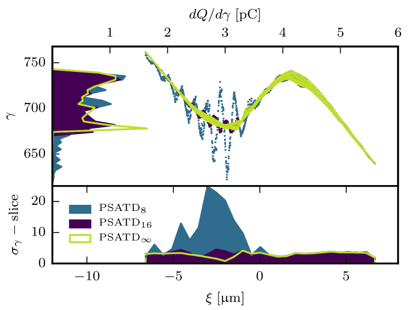
Figure 5: Longitudinal phase space of the witness beam after propagation through $35\,\mathrm{mm}$ of plasma. $\xi$ is the internal bunch coordinate with $\xi=0$ at the center of the witness beam. For decreasing stencil order it is increasingly spoiled by a high frequency oscillation. This causes a growth of projected and slice energy spread (slice length of $0.5\;\mathrm{\upmu m}$ here).

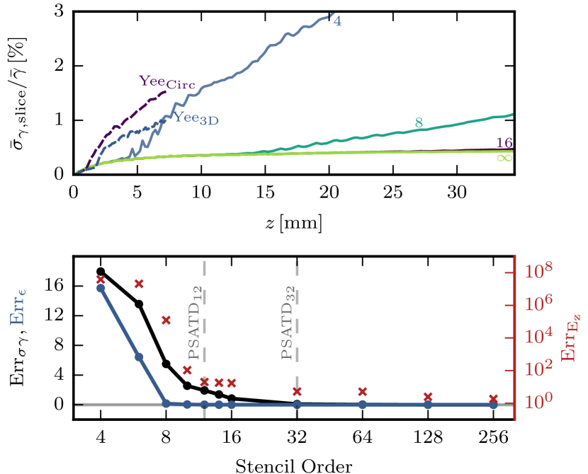
Figure 6: Top: Growth of the witness beam’s slice energy spread during the propagation through $35\,\mathrm{mm}$ of plasma. The slice energy spread is averaged over all slices within $\pm$ 3 standard deviations around the bunch center. The solid and dashed lines show data obtained with the PSATD and Yee scheme, respectively. The PSATD₁₆ and PSATD_∞ lines almost overlay each other. Bottom: Errors in emittance (blue), slice energy spread (black) and longitudinal field (red crosses) after $35\,\mathrm{mm}$. For a stencil order increasing from 4 to 256 the error introduced by NCR in the electric field decreases by 8 orders of magnitude. Consequently, the error of the final emittance and slice energy spread quickly approaches zero.

The stencil order necessary to meet this criterion depends on the physical and numerical parameters of the simulation. Fig. 7 is obtained from scans over the beam charge, the propagation length as well as the longitudinal grid resolution and shows the required stencil order to achieve $\mathrm{Err}_{\sigma\gamma}<0.05$. Fig. 7 (top) shows the required stencil order depending on the propagation length in plasma for the same parameters used in Fig. 3-6. For a reduced propagation length accurate modeling is possible with lower stencil orders. This is a result of the difference in the growth rate of the spurious slice energy spread seen in Fig. 6 (top).
NCR also scales with the bunch charge density and the longitudinal grid resolution. The connection of the required stencil order with these parameters is shown in Fig. 7 (bottom). As the computational demand increases quadratically with the grid resolution, this scan and for consistency also the charge scan are evaluated after a propagation length of $20$ mm. Clearly, high charges call for increased stencil orders (see Fig. 7b). However, please note that in the presented case, due to the small beam dimensions $50$ pC already correspond to a high peak current of $3$ kA and a peak electron density of $1\times 10^{19}\;\mathrm{cm}^{-3}$.
The required stencil order can be reduced by increasing the longitudinal grid resolution (see Fig. 7c). However, for the propagation length and charge considered here, it is necessary to apply a stencil order of at least 8 even when using a resolution of 20 cells/$\upmu$m.

Figure 7: Starting from the parameters used in Fig. 3-6 either the charge, the propagation length or the longitudinal grid resolution is scanned and the required stencil order to fulfill $\mathrm{Err}_{\sigma\gamma}<0.05$ is shown. Top: Required stencil order depending on the propagation length for a beam charge of $50$ pC and a resolution of $5$ cells/$\upmu$m. Bottom: Required stencil order depending on the beam charge (b) with a resolution of $5$ cells/$\upmu$m, and depending on the longitudinal grid resolution (c) with a beam charge of $50$ pC, both evaluated after $20$ mm of propagation in plasma.

Conclusion

In conclusion, NCR stemming from erroneous modeling of the dispersion relation leads to beam phase space degradation, which manifests itself in a spurious growth of slice energy spread and emittance. This effect is present in both the FDTD Yee scheme and finite order PSATD solvers. Errors from NCR rapidly decrease for higher stencil orders, eventually showing the same results as the NCR-free infinite order PSATD solver.
In the case discussed here, which is inspired by typical beam driven plasma acceleration parameters, a stencil order of 32 effectively suppresses spurious beam quality degradation. We have chosen a long propagation distance of 35 mm and a high witness beam charge of 50 pC corresponding to an electron density of $1\times 10^{19}$ cm^-3. This is a conservative example in the sense that our results are applicable to many setups in the field of plasma acceleration that use more moderate parameters. This is confirmed by parameter scans that show that the constraints on the required stencil order are relaxed for a lower beam charge and shorter propagation length.
In practice, this means that with around $60$ guard cells between neighboring domains, parallelization is possible while retaining the physics of the considered problem.
Analogous to the frequently used Yee scheme, growth of NCR in the finite order stencil PSATD scheme can also be reduced by increasing the resolution of the simulation grid. However, this is an inefficient solution especially in schemes where the timestep is limited by a CFL-condition and hence directly linked to the grid resolution. Yet, this means that in simulations with high spatial resolution the effects of NCR are less severe. This, for example, would be the case for laser plasma acceleration, where a high resolution is required in any case to resolve the laser wavelength. Therefore, in these cases even lower order stencils than suggested here are sufficient to model the physics without artifacts from NCR.
The arbitrary order PSATD scheme preserves the benefits of pseudo-spectral solvers, e.g. the analytic integration in time or a centered definition of the electric and magnetic fields. It further allows to independently adjust the precision of the electromagnetic dispersion relation and the resolution of the simulation. This way the needed spatial resolution is governed by the physical problem and not by the mitigation of NCR.

Input scripts to reproduce the presented Fbpic and Warp simulations can be found in Ref. Jalas et al. (2017).