From cells to tissue: A continuum model of epithelial mechanics

Abstract

A continuum model of epithelial tissue mechanics was formulated using cellular-level mechanical ingredients and cell morphogenetic processes, including cellular shape changes and cellular rearrangements. This model can include finite deformation, and incorporates stress and deformation tensors, which can be compared with experimental data. Using this model, we elucidated dynamical behavior underlying passive relaxation, active contraction-elongation, and tissue shear flow. This study provides an integrated scheme for the understanding of the mechanisms that are involved in orchestrating the morphogenetic processes in individual cells, in order to achieve epithelial tissue morphogenesis.

I Introduction

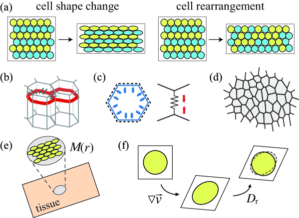
Figure 1: Schematic illustration of the model of epithelial mechanics. (a) Tissue deformation based on cellular shape deformation (left) and by cellular rearrangement (right). (b) In epithelial tissues, cells adhere to each other via E-Cadherin (green) at adherens junctions (AJ), and acto-myosin (red) runs along the cell junctions. (c) Cell pressures (left) and cell junction tensions (right) act in the AJ plane and determine epithelial cell shapes. (d) CVM schematic representation. Each cell is represented by a polygonal contour. (e, f) Schematic illustration of the model presented here. (e) A coarse-grained cellular shape tensor $M$ represents the tissue-scale cellular shape field in our model. (f) Kinematics of cellular shape deformation. Cellular shape alterations through tissue deformation $\nabla\vec{v}$ and cell rearrangement $D_{\mathrm{r}}$.

During tissue morphogenesis, tissues acquire their unique shape and size through a series of deformations. Morphogenesis occurs at multiple levels, and molecular, cellular, and tissue level changes are interdependent. At cellular level, tissue deformation is accounted for by changes in cell shape, position, and number (Fig. 1(a); hereafter named cell morphogenetic processes), which are triggered by biochemical signaling and forces generated by cells Heisenberg2013 ; Sampathkumar2014 ; Guillot2013 . While the tissue stress can affect cell morphogenetic processes through the changes in molecular activity and localization, cell morphogenetic processes generate stress Blanchard2011 ; Aigouy2010 ; Sugimura2013 ; Aw2016 ; Uyttewaal2012 ; Schluck2013 ; Wyatt2015 . However, the mechanisms by which the shape of a tissue emerges from these multi-scale feedback processes remain unclear.

In order to clarify this, a coarse-grained description and modeling of cellular and tissue dynamics at an appropriate length scale is required: while the position and timing of cell morphogenetic processes are stochastic at single cell level, the averaging of values obtained over a larger length scale yields a smooth spatial pattern that is reproducible among different samples. We previously determined the appropriate averaging length scale for describing epithelial tissue dynamics (several tens of cells in a patch), and developed coarse-grained methods for measuring stress and kinematics Bosveld2012 ; Guirao2015 ; Ishihara2012 ; Ishihara2013 . A force inference method was used for the quantification of cell junction tensions and cell pressures (Fig. 1(b), (c)), which can be integrated to calculate a stress tensor Ishihara2012 ; Ishihara2013 ; Chiou2012 ; Brodland2014 . A texture tensor method was used for the measuring of different cell morphogenetic processes (e.g., cell division, cell shape changes) in the same physical dimension, which can be further integrated to obtain tissue scale, spatio-temporal maps of tissue growth and cell morphogenetic processes Guirao2015 . Together, these methods provide the information on the amplitude, orientation, and anisotropy of tissue stress, tissue growth, and cell morphogenetic processes, and correlations between them Guirao2015 .

A modeling scheme capable of accommodating the quantitative data described above is still lacking Khalilgharibi2016 . Cell-based models, such as the cell vertex model (CVM) Honda1983 and the cellular Potts model (CPM) Graner1993 are often employed for the simulation of epithelial tissue morphogenesis (Fig. 1(d); Fletcher2014 ; Maree2007 ; Brodland2004 ), and have proven useful for including experimental data obtained at cellular level, such as the laser ablation of cell junctions or subcellular distribution of proteins. However, the relationship between cell morphogenetic processes and tissue scale deformation and rheology emerges from numerical simulations without being directly tractable. Continuum models allow the in-depth analysis of tissue rheology Fung1993 ; Tlili2015 , yet in many cases do not include the information of the cellular structure by construction, and thus fail to discriminate between different cell morphogenetic processes. A limited number of studies considered the degrees of freedom that represent cell morphogenetic processes and cell polarity Shraiman2005 ; Ranft2010 ; Tlili2015 ; Popovic2016 , but do so in the context of macroscopic models, which do not incorporate cell-level mechanical parameters explicitly. The finite-element model introduced in Brodland2006 includes at a coarse-grained level the contributions of cellular rheology, shape changes, rearrangements and divisions. A continuum model has been derived from the CVM previously but without considering cell rearrangements Murisic2015 (see also Turner2005 ; Fozard2010 in 1D).

The main aim of our study was to develop a two-dimensional hydrodynamic model of the epithelial tissue. This model included a field that represents coarse-grained cell shape, which enabled us to treat different types of cell morphogenetic processes distinctively. First, kinematics was identified by decomposing tissue deformation into cell shape changes and cell rearrangements. Following this, by introducing an energy function deduced from CVM/CPM, thermodynamic formalism was employed to determine kinetics. The model we derived here describes tissue deformation through stress and deformation tensors, which can be compared with the data obtained experimentally Guirao2015 ; Ishihara2012 ; Ishihara2013 , and can incorporate active terms smoothly. We solved the model for several conditions typical for deforming planar tissues during development, and demonstrated that the model predicts the relaxation of cellular shape following the tissue stretching, the relation of the direction of cell elongation and tissue flow during active contraction-elongation (CE), and shear-thinning in tissues. Our approach provides a theoretical framework that enables to assess how cellular level mechanical parameters and cell morphogenetic processes are integrated to realize tissue-scale deformation.

II Model

II.1 Cellular shape tensor

To construct a continuum model, we approximated each cell by an ellipse, characterized by a $2\times 2$ symmetric tensor $M$. Cellular shape can be expressed as $(\vec{r}-\vec{r}_{c})^{T}M^{-1}(\vec{r}-\vec{r}_{c})=1$, where $\vec{r}_{c}$ represents the center of a cell and superscript ^T denotes the transpose (Fig. 1(e)). Since the eigenvalues of $M$ are the square lengths of ellipse semi-axes, cell area can be presented as $A=\pi|M|^{1/2}$, where $|M|$ is the determinant of $M$. By coarse-graining over a representative surface element comprising a sufficient number of cells Bosveld2012 ; Guirao2015 , we obtained a spatially smooth tensor field $M(\vec{r})$. Similar to a previously described texture tensor Guirao2015 , the symmetric tensor $M(\vec{r})$ represents measure of tissue scale deformation in our model, with the physical dimension of square length, which can be experimentally quantified from segmented images of two-dimensional (2D) epithelia.

II.2 Kinematics

Total tissue deformation rate can be represented by the tensor $\nabla\vec{v}$, in which $\vec{v}$ is the velocity field. Here, we used $\left(\nabla\vec{v}\right)_{ij}=\partial_{j}v_{i}$, where indices $i$ and $j$ denote cartesian coordinates. The deformation rate $\nabla\vec{v}$ represented the sum of its symmetric part $D=(\nabla\vec{v}+[\nabla\vec{v}]^{T})/2$ and its antisymmetric part $\Omega=\left(\nabla\vec{v}-[\nabla\vec{v}]^{T}\right)/2$. We decomposed tissue deformation rate into the sum of contributions, due to the cellular shape alterations and other cell morphogenetic processes, and here, we considered cell rearrangement, division, and death:

$$\nabla\vec{v}=\Omega+D_{\mathrm{s}}+D_{\mathrm{r}}\,.$$ (1)

The quantity $\Omega+D_{\mathrm{s}}$ represents the tissue deformation rate stemming from cellular shape alterations, while $D_{\mathrm{r}}$ denotes the deformation rates that involve topological changes in a network of cell junctions, i.e. cell rearrangement, division, and death. We assumed that these processes are irrotational, so that $D_{\mathrm{r}}$ is symmetric. In practice, these tensors can be experimentally determined by cellular shape tracking Guirao2015 . In cellular materials, $D_{\mathrm{r}}$ is kinematically associated with cell shape changes Tlili2015 :

$$\dot{M}-(\nabla\vec{v}-D_{r})M-M(\nabla\vec{v}-D_{r})^{T}=0\,,$$ (2)

where $\dot{M}\equiv\partial_{t}M+\vec{v}\nabla M$ represents the Lagrange derivative of $M$ (Fig. 1(f)). The kinematic relationship (47) was derived for the non-affine deformation in the rheology of polymer melts Leonov1976 ; Leonov1987 ; Larson1988 and foams Marmottant2008 ; Benito2008 , where $D_{\mathrm{r}}$ can be interpreted as due to the slippage between polymer molecules and between bubbles, respectively. When $D_{\mathrm{r}}=0$, the left-hand side of (47) becomes the co-deformational upper-convected derivative Larson1983 . In SI Section 3, we demonstrate that the conservation of cell number density $\rho=1/\pi|M|^{1/2}$ can be presented as $\partial_{t}\rho+\nabla\cdot(\rho\vec{v})=(\mbox{Tr$\,{D_{\mathrm{r}}}$})\rho$, where Tr  denotes the trace, and Tr$\,{D_{\mathrm{r}}}$ coincides with the variation rate of $\rho$. The effects of cell division and cell death should be investigated in future studies, while here we considered a situation in which individual cells only deform elastically and/or intercalate, and the tissue area is invariant and the deformation rate is traceless ($\mbox{Tr$\,{D_{\mathrm{r}}}$}=0$).

II.3 Energy function and elastic stress

In CVM and CPM, cell geometry can be determined by minimizing energy function Fletcher2014 ; Farhadifar2010

$$f_{c}=\sum_{i}\frac{K}{2}\left(A_{i}-A_{0}\right)^{2}+\sum_{[ij]}\gamma_{0}\ell_{ij}+\sum_{i}\frac{\kappa_{0}}{2}L_{i}^{2}\,,$$ (3)

where $A_{i}$ and $L_{i}$ represent the area and perimeter, respectively, of cell $i$, and $\ell_{ij}$ is the length of the interface between cells $i$ and $j$. The first term represents cell-area elasticity with elastic modulus $K$ and reference cell area $A_{0}$. The second and third terms represent cell junction tensions, where the tension is given by $\gamma_{0}+\kappa_{0}(L_{i}+L_{j})$.

Here, by using the cell shape tensor $M(\vec{r})$, we considered an energy function for the continuum model, which is comparable with that of the CVM/CPM, (3). For arbitrary semi-axes $a$, $b$, the perimeter of an ellipse can be given by Euler’s formula (see Suppl. Fig. S1) Chandrupatla2010 :

$$L(a,b)=\pi\,\sqrt{2(a^{2}+b^{2})}\,\mathcal{F}\left(\frac{1}{4},-\frac{1}{4};1;h^{2}\right),\,h=\frac{a^{2}-b^{2}}{a^{2}+b^{2}}\,,$$ (4)

where $\mathcal{F}$ is a hypergeometric function. Using the Cayley-Hamilton equation, we derived the identities $a^{2}+b^{2}=\mbox{Tr$\,{M}$}$, $(a^{2}-b^{2})^{2}=\mbox{Tr$\,{M}$}^{2}-4|M|$. Upon coarse-graining (3), we obtained energy density per unit area

$$F=\frac{1}{\pi|M|^{1/2}}\left[\frac{K}{2}\left(\pi|M|^{1/2}-A_{0}\right)^{2}+\frac{\gamma_{0}}{2}L(M)+\frac{\kappa_{0}}{2}\!\ L(M)^{2}\right]\,,$$ (5)

where $L(M)$ is defined for arbitrarily large cellular shape anisotropy by

$$L(M)=\pi\,\sqrt{2\mbox{Tr$\,{M}$}}\,\mathcal{F}\left(\frac{1}{4},-\frac{1}{4};1;1-\frac{4|M|}{(\mbox{Tr$\,{M}$})^{2}}\right)\,.$$ (6)

The total elastic energy was obtained by integration $\mathcal{F}=\int F(M(\vec{r}))\,\mathrm{d}\vec{r}$.

We focused, for simplicity, on conditions close to the isotropic case (see SI Sec. 1.2 for higher-order approximations). Expanding $\mathcal{F}$ close to $a=b$, or $(\mbox{Tr$\,{M}$})^{2}=4|M|$, the zero order energy can be written as

$$F\!=\!\frac{1}{\pi|M|^{1/2}}\!\!\left[\frac{K}{2}\left(\pi|M|^{1/2}-A_{0}\right)^{2}+\frac{\pi\gamma_{0}}{\sqrt{2}}\sqrt{\mbox{Tr$\,{M}$}}+\pi^{2}\kappa_{0}\mbox{Tr$\,{M}$}\right]\,,$$ (7)

from which the elastic stress can be further derived as

$$\sigma_{\mathrm{e}}=K(\pi|M|^{1/2}-A_{0})I+\left(\frac{\gamma_{0}}{\sqrt{2\mbox{Tr$\,{M}$}}}+2\pi\kappa_{0}\right)\,\frac{M}{|M|^{1/2}}\,,$$ (8)

where $I$ is the unit tensor (SI Sec. 1, general case). The first and second terms represent the isotropic pressure $-P^{\mathrm{ce}}I$ due to the area-elasticity of cells, and the cellular shape-dependent stress $\sigma^{\mathrm{T}}$ due to cell junction tensions, respectively. (34) is consistent with the expression of the Batchelor stress tensor Batchelor1970 ; Ishihara2012 ; Ishihara2013 relating tissue-scale stress to cell pressures and cell junction tensions. Note that $\sigma_{\mathrm{e}}$ and $M$ commute, and therefore, share the same eigendirections, which is consistent with our previous observation showing that cells are elongated along the inferred maximal stress direction in Drosophila epithelia Sugimura2013 ; Guirao2015 ; Ishihara2012 .

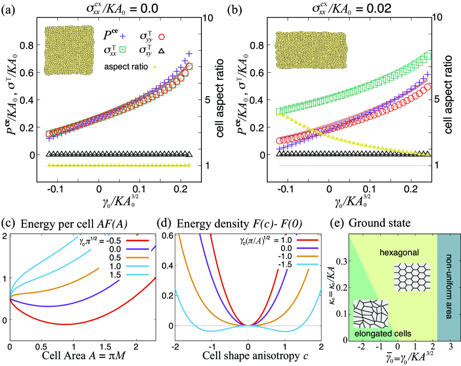
Figure 2: Energy function and elastic stress. (a,b) Macroscopic stress expressions calculated from coarse-grained cellular shape tensor $M$ (symbols) are compared with the true ones (solid lines) obtained using the CVM simulations (left vertical axis), as a function of the non-dimensional parameter $\gamma_{0}/KA_{0}^{3/2}$, with $\kappa_{0}/KA_{0}=0.04$. $P^{\mathrm{ce}}$ and $\sigma^{\mathrm{T}}$ represent the pressure stemming from cell elasticity and the stress generated by cell junction tensions, respectively. Yellow triangles denote the mean cellular shape aspect ratio (right vertical axis), equal to $e^{2c}$ in terms of the cell shape anisotropy. The external stress was set as $\sigma^{\mathrm{ex}}_{xy}=\sigma^{\mathrm{ex}}_{yy}=0$, with (a) $\sigma^{\mathrm{ex}}_{xx}=0$ (isotropic case) and (b) $\sigma^{\mathrm{ex}}_{xx}\neq 0$ (anisotropic case). (c) Energy per cell as a function of the cell area $A$ at $\gamma_{0}\pi^{1/2}=-0.5,0.0,0.5,1.0$ and $1.5$ with $K=1.0$ and $2\pi\kappa_{0}=0.4$. (d) Energy density function $F(c)$ at $\gamma_{0}(\pi/A)^{1/2}=1.0,0.0,-1.0$, and $-1.5$ with $2\pi\kappa_{0}/A=0.6$. (e) A ground state phase diagram is shown as a function of non-dimensional parameters $\overline{\gamma}_{0}=\gamma_{0}/KA^{3/2}$ and $\overline{\kappa}_{0}=\kappa_{0}/KA$, defined using a cell area $A=\pi M_{0}$, instead of $A_{0}$.

We performed numerical simulation of CVM under the isotropic and anisotropic stress environments, and compared the coarse-grained stress with the true one. Coarse-grained cell shape $M$ was evaluated by averaging the second moment of cell shape, and Euler expansion up to the second order was considered (SI Sec. 1.2). The results obtained here confirmed that the coarse-grained stress values agree with those obtained for the true one (Fig. 2(a,b), Suppl. Fig. S2).

Factorizing the tensor $M$ as $M=M_{0}e^{c\Theta}$ can be useful Merkel2017 , and here, $M_{0}$ and $c$ are scalar fields and $\Theta$ is a symmetric, trace-less tensor field parameterized by the angle $\theta$ as

$$\Theta=\begin{pmatrix}\cos 2\theta&~{}\sin 2\theta\\ \sin 2\theta&-\cos 2\theta\end{pmatrix}\,.$$ (9)

Since $\Theta^{2}=I$, we deduced $M=M_{0}[\cosh(c)I+\sinh(c)\Theta]$, where $M_{0}$ quantifies the coarse-grained cell area $A=\pi|M|^{1/2}=\pi M_{0}$, dimensionless parameter $c$ characterizes the coarse-grained cell shape anisotropy, and the angle $\theta$ represents the direction of the major axis of ellipses. Since $\mbox{Tr$\,{M}$}=2M_{0}\cosh(c)$, $L(M)$ and $F(M)$ depend only on $M_{0}$ and $c$.

For the energy function presented in (7), the energy per cell, $A\,F(A,c=0)$, is shown as a function of $A$ in Fig. 2(c) in the isotropic case $c=0$. For large values of $\gamma_{0}$, the functional form becomes concave, indicating thermodynamic instability of the state of homogeneous cell area. Fig. 2(d) shows $F(A,c)$ as a function of $c$ at constant cell area. Circular cell shape ($c=0$) becomes unstable for sufficiently large negative values of $\gamma_{0}$, where cells no longer prefer a hexagonal configuration, but adopt an elongated shape. We recovered two instabilities described for the CVM Farhadifar2010 ; Staple2010 (Fig. 2(e); SI Sec. 1.3), showing that the tissue scale energy density $F(M)$ retains the essential features of the original cell-based models.

II.4 Thermodynamic formalism

Since existing cell-based models, including CVM and CPM, use ad hoc prescriptions for kinetics, we considered the thermodynamic formalism Groot1962 in order to derive generic hydrodynamic equations. The total stress tensor $\sigma$ can be given by the sum of elastic and dissipative stresses, as

$$\sigma=\sigma_{\mathrm{e}}+\sigma_{\mathrm{p}}\,.$$ (10)

The entropy production rate of an isothermal process was calculated as Leonov1976 ; Leonov1987 :

$$T\dot{s}=\sigma\!:\!D-\sigma_{\mathrm{e}}\!:\!D_{\mathrm{s}}=\sigma_{\mathrm{p}}\!:\!D+\sigma_{\mathrm{e}}\!:\!D_{\mathrm{r}}\,,$$ (11)

where $s$ is the entropy density, and $T$ is the temperature. Here, $a\!\!:\!\!b\equiv\mbox{Tr$\,{[ab^{T}]}$}$ denotes the scalar product of two arbitrary tensors $a$ and $b$, and $a^{\prime}\equiv a\!-\!(\mbox{Tr$\,{a}$}/2)I$ is the deviatoric part of $a$. Because $D_{\mathrm{r}}$ is traceless, we can replace $\sigma_{\mathrm{e}}$ by ${\sigma_{\mathrm{e}}}^{\prime}$ in (11). By identifying conjugate flux-force pairs as $\sigma_{\mathrm{p}}$-$D$ and $D_{\mathrm{r}}$-${\sigma_{\mathrm{e}}}^{\prime}$, the fluxes $(\sigma_{\mathrm{p}},D_{\mathrm{r}})$ can be given by using the linear combinations of the forces $(D,{\sigma_{\mathrm{e}}}^{\prime})$:

$$\sigma_{\mathrm{p}} =\chi^{\mathrm{ss}}D-\chi^{\mathrm{sr}}{\sigma_{\mathrm{e}}}^{\prime}\,,$$ (12)

$$D_{\mathrm{r}} =\chi^{\mathrm{rs}}D+\chi^{\mathrm{rr}}{\sigma_{\mathrm{e}}}^{\prime}\,.$$ (13)

The coefficients $\chi^{\mathrm{ss}},\chi^{\mathrm{sr}},\chi^{\mathrm{rs}}$, and $\chi^{\mathrm{rr}}$ are fourth-order tensors that satisfy Onsager’s reciprocity (e.g., $\chi^{\mathrm{sr}}_{ijkl}=\chi^{\mathrm{rs}}_{klij}$). Note that Maxwell’s model was obtained for $\chi^{\mathrm{ss}}=\chi^{\mathrm{sr}}=0$ ($\sigma=\sigma_{\mathrm{e}}$, $\sigma_{\mathrm{p}}=0$), and that Kelvin-Voigt’s model was obtained for $\chi^{\mathrm{rs}}=\chi^{\mathrm{rr}}=0$ ($D=D_{\mathrm{s}}$, $D_{\mathrm{r}}=0$) Leonov1976 ; Leonov1987 . The term $\chi^{\mathrm{ss}}D$ characterizes dissipative stress due to the tissue strain rate, and reduces it to the usual bulk and shear viscous terms for isotropic material. According to (13), cell rearrangements may be driven both by the tissue strain rate and by its elastic stress Aigouy2010 ; Sugimura2013 ; Etournay2015 . The presence of the cross-term $-\chi^{\mathrm{sr}}{\sigma_{\mathrm{e}}}^{\prime}$ in (12) is a non-trivial prediction of the model, which cannot be represented by a rheology diagram in terms of a combination of springs and dashpots.

In the absence of external forces, the above equations can predict the relaxation to the steady state, and are not sufficient to address the active phenomena, such as the sustained epithelial flow Sato2015 or self-organized spatio-temporal patterning Saw2017 . Therefore, we included the formalism of active gels Kruse2005 ; Marchetti2013 , and added the term $r\Delta\mu$ to the entropy production rate (11):

$$T\dot{s}=\sigma_{\mathrm{p}}\!:\!D+{\sigma_{\mathrm{e}}}^{\prime}\!:\!D_{\mathrm{r}}+r\,\Delta\mu\,,$$ (14)

where $\Delta\mu$ represents the change in chemical potential associated with a chemical reaction that supplies energy to the system, and $r$ is the reaction rate. By identifying $r$-$\Delta\mu$ as an additional force-flux pair, additional terms $\sigma_{a}$ and $D_{a}$, which we refer to as active stress and active cell rearrangement, respectively, appeared in (12) and (13), both of which are proportional to $\Delta\mu$.

The coupling coefficients can depend on $M^{\prime}$. Including lowest-order non-linearities, with the condition that $D_{\mathrm{r}}$ is traceless, the generic form of the force-flux relationships can be written as:

$$\sigma_{\mathrm{p}} =\eta\,D^{\prime}+\eta^{\prime}\,(\mbox{Tr$\,{D}$})I$$

$$+\mu\,(DM^{\prime}+M^{\prime}D)+\mu^{\prime}\,(\mbox{Tr$\,{D}$})M^{\prime}+\mu^{\prime\prime}(\mbox{Tr$\,{(DM^{\prime})}$})I$$

$$-\nu_{1}{\sigma_{\mathrm{e}}}^{\prime}-\nu_{2}\left({\sigma_{\mathrm{e}}}^{\prime}M^{\prime}+M^{\prime}{\sigma_{\mathrm{e}}}^{\prime}\right)-\nu_{3}({\sigma_{\mathrm{e}}}^{\prime}\!:\!M^{\prime})I$$

$$-\zeta_{1}\Delta\mu\,I-\zeta_{2}\Delta\mu\,M^{\prime}\,,$$ (15)

$$D_{\mathrm{r}} =\nu_{1}D^{\prime}+\nu_{2}(DM^{\prime}+M^{\prime}D-\mbox{Tr$\,{(DM^{\prime})}$}I)+\nu_{3}(\mbox{Tr$\,{D}$})M^{\prime}$$

$$+\eta^{-1}_{1}{\sigma_{\mathrm{e}}}^{\prime}+\eta^{-1}_{2}\left({\sigma_{\mathrm{e}}}^{\prime}M^{\prime}+M^{\prime}{\sigma_{\mathrm{e}}}^{\prime}-\mbox{Tr$\,{({\sigma_{\mathrm{e}}}^{\prime}M^{\prime})}$}I\right)$$

$$-\beta_{\mathrm{2}}\Delta\mu\,M^{\prime}\,,$$ (16)

where the coupling coefficients are scalar in an isotropic system. In (53), $\eta$ and $\eta^{\prime}$ denote the tissue shear and bulk viscosity, respectively, and $\mu$, $\mu^{\prime}$, and $\mu^{\prime\prime}$ denote their anisotropic correction depending on the cellular shape. The term $\nu_{1}D^{\prime}$ of (54) plays a role similar to that of the Gordon-Schowalter process in the rheology of polymer melts, which describes the relaxation of polymer deformation, and, consequently, stress, by slippage Larson1983 . The cross terms, including $\nu_{2},$ and $\nu_{3}$, are possible in general. We introduced the active stress tensor as $\sigma_{\mathrm{a}}=-\left(\zeta_{1}I+\zeta_{2}M^{\prime}\right)\Delta\mu$. Using the terminology of active nematic liquid crystals, a negative and positive $\zeta_{2}$ values correspond to a contractile and extensile, respectively, material Marchetti2013 . These activities are often attributed to myosin contractility, for which ATP is consumed. The terms coupling $D_{\mathrm{r}}$ and ${\sigma_{\mathrm{e}}}^{\prime}$ in (54) underlie the Maxwellian dynamics of the system, and include the positive coefficient $\eta_{1}$ with the dimension of viscosity. In (54), active cell rearrangements contribute to the constitutive equation for $D_{\mathrm{r}}$ as $D_{\mathrm{a}}=-\beta_{2}\Delta\mu\,M^{\prime}$. Both $\sigma_{\mathrm{a}}$ and $D_{\mathrm{a}}$ are symmetric second-order tensors. Our treatment of active stresses and active cell rearrangements was similar to that suggested previously Etournay2015 ; Popovic2016 , since both approaches are inspired by the active gel models Kruse2005 ; Marchetti2013 .

Finally, the force balance equation was used to close the system:

$$\nabla\cdot\sigma=-\vec{f}_{\textrm{ex}},$$ (17)

where $\vec{f}_{\textrm{ex}}$ represents the external force field, supplemented with the appropriate boundary conditions. Collectively, the constitutive equations (34,10,53,54) with the kinematic relationships (1,47) and the force balance equation (17) determine hydrodynamic equations of a tissue (SI Sec. 2).

III Applications

We investigated three simple examples of dynamical behavior predicted by our model, including the passive response following the axial stretch induced by an external force, the deformation of a tissue due to the active internal forces, and the generation of shear flow. Two assumptions were used for simplicity to obtain the following analytical solutions: 2D incompressibility of a tissue ($M_{0}$ is constant and $\mbox{Tr$\,{D}$}=\mathrm{div}\vec{v}=0$; SI Sec. 2) and spatial homogeneity of all relevant fields.

III.1 Passive relaxation following the axial stretching

In Drosophila pupal wing, an external force from the proximal part of the body is responsible for the stretching of the wing along the proximal-distal (PD) axis. Upon the tissue stretching, wing cells elongate along the PD axis, while the tissue relaxes during several hours when cells intercalate and adopt a less elongated shape Aigouy2010 ; Sugimura2013 ; Guirao2015 ; Etournay2015 . Below, we demonstrated that our model can recapitulate this process, and determined the characteristic relaxation time in terms of cell mechanical parameters.

We considered a tissue with an initial size $L_{x}\times L_{y}=L_{0}\times L_{0}$ and in an initial isotropic, uniform state where the cell shape tensor is $M\!=\!M_{0}\,I$. From time $t=0$, the tissue elongates along the $x$-axis at the constant rate $\dot{L}_{x}/L_{x}=\partial_{x}v_{x}=\lambda$, and consequently, contracts along the $y$-axis at the rate $\dot{L}_{y}/L_{y}=\partial_{y}v_{y}=-\lambda$ (Fig. 3(a)). When the tissue size reaches $aL_{0}\times a^{-1}L_{0}$, the stretching stops ($\partial_{x}v_{x}=\partial_{y}v_{y}=0$). We attempted to identify a uniform solution to the problem, so that (17) is automatically verified when $f_{\textrm{ex}}=0$. All tensor variables are diagonal ($M=M_{0}e^{c\Theta}$ with $\theta=0$ ). The $M$-dependent terms in Eqs (53-54) are either canceled, or are isotropic tensors that may be absorbed into the pressure. Since we consider a passive process here and ignore active terms, we set $\Delta\mu=0$. Using (47), the time evolution of $c$ can be written as:

$$\dot{c}=2(1-\nu_{1})\partial_{x}v_{x}-2\eta^{-1}_{1}\Gamma(c)\sinh(c)\,,$$ (18)

where $\Gamma(c)=\gamma_{0}/2\sqrt{M_{0}\cosh c}+2\pi\kappa_{0}$ represents the strength of cell junction tensions as a function of cell mechanical parameters $\gamma_{0}$ and $\kappa_{0}$. The normal stress components were

$$\sigma_{xx} =-p+\eta\,\partial_{x}v_{x}+(1-\nu_{1})\Gamma(c)\sinh c\,,$$ (19)

$$\sigma_{yy} =-p+\eta\,\partial_{y}v_{y}-(1-\nu_{1})\Gamma(c)\sinh c\,,$$ (20)

where the pressure $p$ was determined in order to satisfy the incompressibility condition.

Setting $a=5$, the time course of cell shape anisotropy $c(t)$ is presented for several values of $\lambda$ in Figure 3(b). When $|c|\ll 1$, the temporal evolution becomes Maxwellian,

$$\dot{c}+2\eta^{-1}_{1}\Gamma(0)\,c=2(1-\nu_{1})\partial_{x}v_{x}.$$ (21)

This equation explicitly relates the relaxation time for cell rearrangements $\tau_{\mathrm{r}}=\eta_{1}/2\Gamma(0)$ to cell mechanical parameters. If the stretch rate is slower than this time scale ($\tau_{\mathrm{r}}<\lambda^{-1}$), the cells remain approximately circular during cell rearrangement, which is in a sharp contrast to transient cell elongation during the more rapid tissue stretch.

Given cell junction tensions of the order of $\gamma_{0}\approx 10^{-10}\,\mathrm{N}$ Bambardekar2015 , and a cellular length scale of the order of $r\approx 10^{-6}$ m, we expected $\Gamma(0)\sim\gamma_{0}/r\approx 10^{-4}\,\mathrm{N}\,\mathrm{m}^{-1}$. Since the time scale for relaxation is of the order of a few hours, $\tau_{\mathrm{r}}\approx 10^{4}\,\mathrm{s}$ Aigouy2010 ; Sugimura2013 , we obtained the order of magnitude of the 2D viscosity coefficient $\eta_{1}\sim\Gamma(0)\tau_{\mathrm{r}}\approx 1$ Pa m s. For comparison, we expected a 2D shear viscosity of the order of $\eta\approx 1\,\mathrm{Pa}\,\mathrm{m}\,\mathrm{s}$, provided by $\eta=h\,\eta_{3\mathrm{D}}$, where $h\approx 10^{-5}\,\mathrm{m}$ represents the typical height of the epithelium and $\eta_{3\mathrm{D}}\approx 10^{5}\,\mathrm{Pa}\,\mathrm{s}$ was determined in vitro in cell aggregates Guevorkian2010 ; Stirbat2013 .

III.2 Active contraction-elongation (CE)

CE denotes the simultaneous shrinkage and expansion of a tissue along two orthogonal axes Tada2012 , often controlled by the anisotropic localization/activity of signaling/driving molecules, such as molecular motors Guillot2013 ; Heisenberg2013 ; Bosveld2012 ; Shindo2014 ; Rozbicki2015 . During the CE, cells are often elongated along the axis perpendicular to the direction of the tissue flow (Fig. 4(a)) Tada2012 ; Shindo2014 ; Rozbicki2015 ; Morishita2017 which may occur in order to facilitate the force transmission along the axis of tissue contraction, through the formation of multicellular myosin cables through the mechanosensing of neighboring cells Rozbicki2015 . However, the mechanisms whereby tissue deformation due to the cellular shape alterations counteract that due to the cell rearrangements remain unclear.

Here, we investigated the CE by extending our model to include active stress and rearrangements provided by signaling molecules oriented along a fixed direction, as represented by a traceless tensor $Q=\vec{n}\otimes\vec{n}-\mbox{Tr$\,{(\vec{n}\otimes\vec{n})}$}/2$, where $\vec{n}=(\cos\phi,\sin\phi)^{T}$ represents a unit vector field pointing to the direction $\phi$. Possible feedbacks on the signal activity were ignored. We considered the lowest-order active contributions

$$\sigma_{\mathrm{a}} =-\zeta_{1}\,\Delta\mu\,I-\zeta_{\mathrm{Q}}\,\Delta\mu\,Q\,,$$ (22)

$$D_{\mathrm{a}} =-\beta_{\mathrm{Q}}\,\Delta\mu\,Q\,,$$ (23)

where the parameters $\zeta_{\mathrm{Q}}$ and $\beta_{\mathrm{Q}}$, respectively, quantify the strength of the active stress and of the active rearrangements. Negative and positive $\zeta_{\mathrm{Q}}$ values correspond to the contractile and extensile, respectively, stress along the direction $\vec{n}$. For positive $\beta_{\mathrm{Q}}$, $D_{\mathrm{a}}$ drives cell rearrangements where a cell junction parallel to $\vec{n}$ shrinks and is remodeled to form a new cell junction perpendicular to $\vec{n}$. As above, $-\zeta_{1}\,\Delta\mu\,I$ is absorbed into the pressure term when the tissue is incompressible.

We considered a uniform and fixed signal $\vec{n}=(0,1)^{T}$. We set $\zeta_{2}=\beta_{2}=0$ to focus on the activity induced by $Q$ (SI Sec. 3.1 for full calculation). Assuming as above that $\theta=0$, Eqs. (18-20) become

$$\dot{c} =2(1-\nu_{1})\partial_{x}v_{x}-2\eta^{-1}_{1}\Gamma(c)\sinh c-\beta_{\mathrm{Q}}\Delta\mu$$ (24)

$$\sigma_{xx} =-p+\eta\,\partial_{x}v_{x}+(1-\nu_{1})\Gamma(c)\sinh c+\frac{\zeta_{\mathrm{Q}}}{2}\Delta\mu$$ (25)

$$\sigma_{yy} =-p+\eta\,\partial_{y}v_{y}-(1-\nu_{1})\Gamma(c)\sinh c-\frac{\zeta_{\mathrm{Q}}}{2}\Delta\mu\,.$$ (26)

In isotropic stress conditions ($\sigma_{xx}=\sigma_{yy}$), both the cellular shape anisotropy at steady state ($\dot{c}=0$), determined by:

$$\Gamma(c)\sinh c=-\frac{(1-\nu_{1})\eta_{1}\zeta_{\mathrm{Q}}+\eta\eta_{1}\beta_{\mathrm{Q}}}{\eta_{1}(1-\nu_{1})^{2}+\eta}\frac{\Delta\mu}{2}\,,$$ (27)

and the tissue deformation rate $\partial_{x}v_{x}$

$$\partial_{x}v_{x}=\frac{-\zeta_{\mathrm{Q}}+(1-\nu_{1})\eta_{1}\beta_{\mathrm{Q}}}{\eta_{1}\left(1-\nu_{1}\right)^{2}+\eta}\frac{\Delta\mu}{2}\,.$$ (28)

remain non-zero, indicating that the tissue anisotropy and flow are maintained through the active stresses and cell rearrangements. In Eqs. (27) and (28), cellular shape anisotropy $c$ and velocity gradient $\partial_{x}v_{x}$ may adopt either an identical or an opposite sign depending on the numerical values of the active coefficients $\beta_{\mathrm{Q}}$ and $\zeta_{\mathrm{Q}}$. Therefore, cell elongation occurs either parallel or perpendicular to the direction of flow, depending on the parameter values (phase diagram in Fig. 4(b), with $\nu_{1}<1$). Considering the contractile effect of myosin motors (upper right quadrant of Fig. 4(b), $-\zeta_{\mathrm{Q}}>0$ and $\beta_{\mathrm{Q}}>0$), cell elongation occurs mostly perpendicular to the tissue flow, except below the green line of the slope $(1-\nu_{1})/\eta$. An earlier study using CPM suggested that the differential cell adhesion accounts for CE with cell elongation orthogonal to tissue flow, in which only the outer tissue boundary contributes to the driving of tissue deformation Zajac2000 ; Zajac2003 . Our model provides an alternative mechanism in which activities play an essential role, in agreement with recent observations of elevated myosin activity in the elongated cell junctions orthogonal to the tissue flow Shindo2014 ; Rozbicki2015 .

III.3 Shear flow

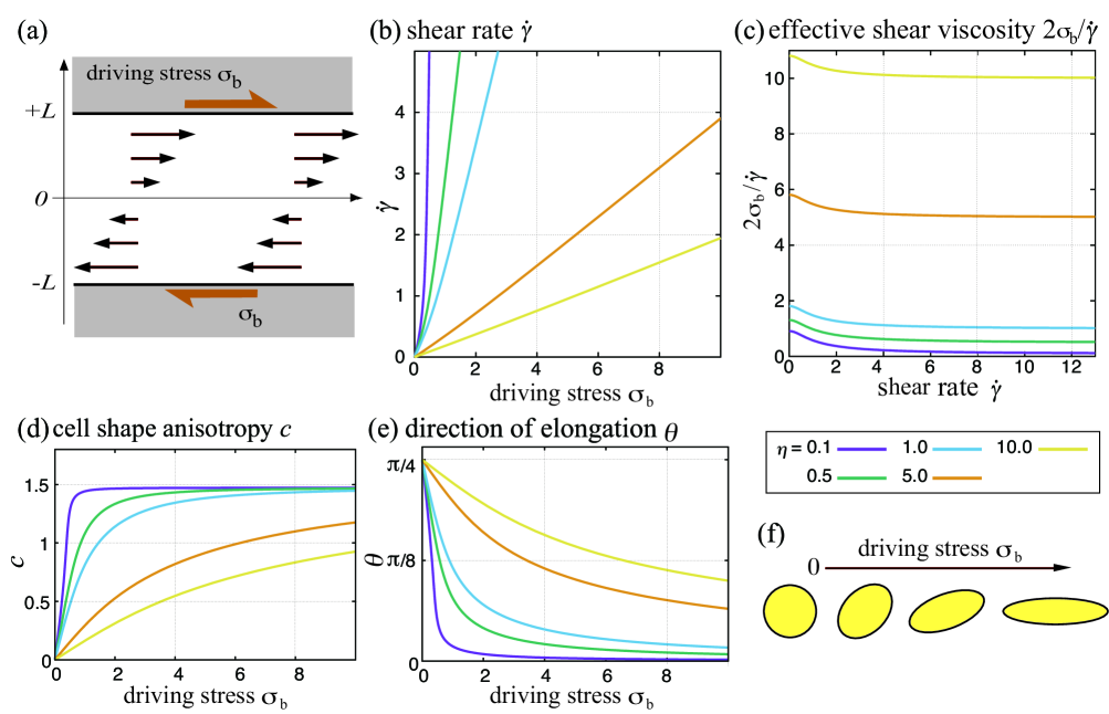
Figure 5: The tissue behaving as a shear-thinning fluid. (a) An external shear stress ($\sigma_{\mathrm{b}}$) is applied at the top and bottom boundaries ($y=\pm L$). (b) The shear rate $\dot{\gamma}$ is plotted against the driving stress $\sigma_{\mathrm{b}}$. (c) The effective viscosity $2\sigma_{\mathrm{b}}/\dot{\gamma}$ decreases as a function of the shear rate $\dot{\gamma}$. Cell shape anisotropy $c$ (d) and orientation $\theta$ (e) are plotted as a function of the driving stress $\sigma_{\mathrm{b}}$. (f) Cells elongate and align along the force axis as the driving stress $\sigma_{\mathrm{b}}$ increases. Parameters were set as $\gamma_{0}/(4M_{0})^{1/2}=0.1\,\mathrm{mN}\,\mathrm{m}^{-1}$, $2\pi\kappa_{0}=0.4\,\mathrm{mN}\,\mathrm{m}^{-1}$, $\nu_{1}=0.1$ and $\eta_{1}=1.0\,\mathrm{Pa}\,\mathrm{m}\,\mathrm{s}$.

A fundamental geometry for investigating rheology Oswald2009 , shear flow is commonly found in many developmental tissues Guirao2015 ; Sato2015 ; Rozbicki2015 . Here, we considered the simple geometry given in Fig. 5(a), inspired by the plane Couette flow Oswald2009 . The flow, with shear rate $\dot{\gamma}=\partial_{y}v_{x}$, is driven by an external shear stress $\sigma_{\mathrm{b}}$ acting in the opposite directions on the boundaries. The effective shear viscosity $\eta_{\mathrm{eff}}$ can be calculated as:

$$\eta_{\mathrm{eff}}=\frac{2\sigma_{\mathrm{b}}}{\dot{\gamma}}=\eta+(1-\nu_{1})^{2}\eta_{1}-(1-\nu_{1})\eta_{1}\cos 2\theta\tanh c\,,$$ (29)

where the cell shape anisotropy $c$ and orientation $\theta$ depend on the driving stress $\sigma_{\mathrm{b}}$ (SI Sec. 3.2). In the presence of a coupling between the cellular rearrangement rate and the elastic stress ($\eta_{1}\neq 0$), $\eta_{\mathrm{eff}}$ depends on $\sigma_{\mathrm{b}}$, which makes the tissue non-Newtonian (Fig. 5). The shear rate is an increasing function of the external stress $\sigma_{\mathrm{b}}$, whereas the effective shear viscosity decreases with $\dot{\gamma}$, indicating that the model predicts shear-thinning (Fig. 5(b-c)). Cellular shape anisotropy $c$ increases with $\sigma_{\mathrm{b}}$ or $\dot{\gamma}$, to converge to a finite value for large driving. Cells turn in the direction of the applied stress as they elongate (Fig. 5(d-f)). Shear-thinning was reported in vitro, using cellular spheroids Marmottant2009 , and was shown to be related to stress-dependent barriers that may control cell rearrangements (see Marchetti2013 for a mechanism leading to shear-thinning in active materials that does not involve topological effects). To the best of our knowledge, there is no experimental evidence for the shear-thinning in epithelial tissues in vivo, which is a non-trivial prediction of our model, obtained assuming only linear force-flux couplings.

Including the active stress and active cell rearrangements, both internal, Eqs. (53-54), or due to an oriented signal, Eqs. (22-23), the shear rate becomes

$$\dot{\gamma}=2\,\frac{\sigma_{\mathrm{b}}+\sigma_{2}+\sigma_{\mathrm{Q}}}{\eta+(1-\nu_{1})^{2}\eta_{1}-(1-\nu_{1})\eta_{1}\cos 2\theta\tanh c}\,,$$ (30)

with $\sigma_{2}=\Delta\mu\,M_{0}\,\sinh c\,\sin 2\theta(\zeta_{2}-2\eta_{1}(1-\nu_{1})\beta_{2})$ and $\sigma_{\mathrm{Q}}=\Delta\mu\,\sin 2\phi(\zeta_{\mathrm{Q}}+\eta_{1}(1-\nu_{1})\beta_{\mathrm{Q}})$. In addition to the external stress $\sigma_{\mathrm{b}}$, active stresses and active cell rearrangements are able to drive shear flow. Indeed, the active rearrangements described by (23) produce shear flow for an arbitrary orientation $\phi$, as has been observed in the genitalia of Drosophila and demonstrated using the CVM in the case of $\vec{n}$ pointing to $\phi=3\pi/4$ Sato2015 .

IV Discussion

We formulated a continuum model of epithelial mechanics based on the definition of a tissue-scale field $M$ representing cellular shape. The advantages of using this approach are as follows. Most importantly, our model is designed to connect cellular level mechanical ingredients (e.g., cell area elasticity and cell junction tension) and cell morphogenetic processes (e.g., cell rearrangements), in order to drive tissue mechanics and deformation. This was achieved by defining the energy function and kinematic relationship in terms of the cell shape field $M$, which distinguishes our work from the previous continuum models Tlili2015 ; Popovic2016 ; Brodland2006 . The model describes time-dependent flows, and allows the evaluation of time scales as a function of material parameters. Large and non-affine deformations can be treated. In addition, the model can also incorporate a signal field, for instance, the axial tensor $Q$, which, here, orients active stresses and cellular rearrangements. Many relevant fields can be experimentally determined, including tissue stress, tissue deformation, cell morphogenetic processes, and chemical signaling fields, such as the concentrations of cell polarity molecules or the orientation field describing the spatial distribution of myosin molecules. Once their dynamics are quantitatively characterized by the relevant scalar, vector, or tensor variables Aigouy2010 ; Sugimura2013 ; Bosveld2012 ; Guirao2015 ; Ishihara2012 ; Blanchard2009 ; Etournay2015 ; Blanchard2017 , comparison between the model and experiments is feasible.

The data presented here demonstrate that using our model, we can predict the dynamical behaviors underlying epithelial tissue morphogenesis. In the future, the quantitative comparison of the model predictions with experimental data should help us evaluate material parameters and validate constitutive equations. For example, since $D$, $D_{\mathrm{r}}$ Guirao2015 and $\sigma_{\mathrm{e}}$ Ishihara2012 ; Ishihara2013 are measurable quantities, the validity of (13) can be tested by comparing it with the experimental data. Furthermore, the relevance of the non-linear terms in (54) for epithelial rheology may be tested.

The current approach can be extended in several ways. Other cell morphogenetic processes, such as cell division and cell death, should be incorporated to the current modeling scheme Yabunaka2017 . Plastic behavior Marmottant2009 may be considered as well, either within the dissipation function formalism Tlili2015 , or by considering non-linear constitutive equations to effectively incorporate a yield stress. In analogy to the recent adaptations of the CPM Kabla2012 or the CVM Barton2016 , a cell polarity field may be included to describe collective cell migration Yabunaka2017 . Another possible extension of the model concerns kinetics. Here, the associated dissipation coefficients, including the coefficients governing active stress and active rearrangement, were determined phenomenologically by employing the thermodynamic formalism. This point can be further explored by considering detailed processes at the cellular level. In particular, the cell-level machinery underlying tissue-level active processes should be studied further in connection with signal activity dynamics. Finally, our 2D formalism can be extended to 3D.

In conclusion, the present work provides an integrated scheme for the understanding of the mechanical control of epithelial morphogenesis. Dynamics of signal fields can be coupled to the equations. Feedback between biochemical signaling and mechanics through the mechanosensing of a cell Blanchard2011 ; Aigouy2010 ; Sugimura2013 ; Aw2016 ; Uyttewaal2012 may represent a potential future research direction.

acknowledgements

We thank Yohanns Bellaïche, Cyprien Gay, François Graner, Boris Guirao, and Shunsuke Yabunaka for discussion. This research was supported by JSPS KAKENHI Grant Number JP24657145 and JP25103008, the JST CREST (JPMJCR13W4), the JST PRESTO program (13416135), and by the JSPS/MAEDI/MENESR Sakura program.

Appendix A Energy function and elastic stress

A.1 Derivation of elastic stress

The shape of a given cell is represented by $(\vec{r}-\vec{r}_{c})^{T}\,M^{-1}\,(\vec{r}-\vec{r}_{c})=1$, where $M$ is a positive definite matrix, and the center of the cell is located at $\vec{r}_{c}$.

Let each material point at the position $\vec{r}$ move to $\vec{r^{\prime}}=\vec{r}+\vec{u}(\vec{r})$, thus defining the displacement field $\vec{u}$. The center of a cell changes as $\vec{r^{\prime}}_{c}=\vec{r}_{c}+\vec{u}(\vec{r}_{c})$ and the cell shape changes as

$$(\vec{r}-\vec{r^{\prime}}_{c})^{T}\left((1+\nabla\!\vec{u})^{-1}\right)^{T}M^{-1}(1+\nabla\!\vec{u})^{-1}(\vec{r}-\vec{r^{\prime}}_{c})=1\,.$$

Upon coarse-graining, this indicates that $M$ changes as

$$M^{\prime}(\vec{x}+\vec{u})=(1+\nabla\vec{u})M(\vec{x})(1+\nabla\vec{u}^{T})\,,$$

whereby, at order $\mathcal{O}(|\nabla\vec{u}|)$,

$$M\to M^{\prime}=M-\vec{u}\cdot\nabla M+M(\nabla\!\vec{u})^{T}+\nabla\vec{u}M\,.$$ (31)

This equation represents the relationship between the change in the cell shape and tissue displacement field, in the absence of cell rearrangements. It has been derived rigorously for a cellular material in Tlili2015 .

By the virtual displacement $\vec{u}$, the total energy $\mathcal{F}(M)=\int F(M)\mathrm{d}\vec{x}$ changes as follows:

$$\delta\mathcal{F} =\mathcal{F}(M^{\prime})-\mathcal{F}(M)\simeq\int\frac{\partial F}{\partial M}:\delta M\mathrm{d}\vec{x}$$

$$=\int\frac{\partial F}{\partial M}:\left(-\vec{u}\cdot\nabla M+M(\nabla\!\vec{u})^{T}+\nabla\vec{u}M\right)\mathrm{d}\vec{x}$$

$$=\int\left[-\nabla\!\cdot\!(\vec{u}F)+\left(FI+\left(\frac{\partial F}{\partial M}\right)^{T}M+\frac{\partial F}{\partial M}M^{T}\right):\nabla\vec{u}\right]\mathrm{d}\vec{x}$$

where $I$ represents the unit tensor and $\delta M=M^{\prime}-M$. The first term vanishes at the boundary of the system, and the elastic stress $\sigma_{\mathrm{e}}$ is given as:

$$\sigma_{\mathrm{e}}=FI+\left(\frac{\partial F}{\partial M}\right)^{T}M+\left(\frac{\partial F}{\partial M}\right)M^{T}\,,$$ (32)

Since $M$ is symmetric, this expression further simplifies to

$$\sigma_{\mathrm{e}}=FI+2\left(\frac{\partial F}{\partial M}\right)M\,.$$ (33)

Using the relations

$$\frac{\partial{}}{\partial{M}}\mbox{Tr$\,{M}$}=I,\quad\frac{\partial{}}{\partial{M}}|M|=|M|M^{-1}\,,$$

and given Eq. (7) for the expression of the energy, Eq. (33) leads to

$$\sigma_{\mathrm{e}}=K(\pi|M|^{1/2}-A_{0})I+\left(\frac{\gamma_{0}}{\sqrt{2\mbox{Tr$\,{M}$}}}+2\pi\kappa_{0}\right)\,\frac{M}{|M|^{1/2}}\,.$$ (34)

A.2 Comparison of macroscopic and microscopic stress

To check the validity of coarsening, we conducted numerical simulation of CVM with an energy function given by Eq. (3) in the main text Farhadifar2010 ; Fletcher2014 :

$$f_{c}=\sum_{i}\frac{K}{2}\left(A_{i}-A_{0}\right)^{2}+\sum_{[ij]}\gamma_{0}\ell_{ij}+\sum_{i}\frac{\kappa_{0}}{2}L_{i}^{2}\,,$$ (35)

and compared two expressions of the stress tensor.

The first one is the ‘microscopic’ expression directly calculated from CVM Ishihara2012 ; Ishihara2013 ; Guirao2015

$$\sigma^{\mathrm{CVM}}=\frac{1}{\sum_{i}A_{i}}\left(-\sum_{i}P_{i}A_{i}I+\sum_{[ij]}T_{ij}\frac{\ell_{ij}\otimes\ell_{ij}}{|\ell_{ij}|}\right)\,$$ (36)

where $A_{i}$ is the area of cell $i$, and $\ell_{ij}$ is the length of the interface between cells $i$ and $j$. $P_{i}$ is the pressure of $i$-th cell originating from cell elasticity, and $T_{ij}$ is the tension of cell interface $[ij]$. $P_{i}$ and $T_{ij}$ are determined from the above energy function as $P_{i}=-K(A_{i}-A_{0})$ and $T_{ij}=\gamma_{\mathrm{0}}+\kappa_{\mathrm{0}}\left(L_{i}+L_{j}\right)$.

The second one is the ‘macroscopic’ expression of stress obtained by coarse-grained cell shape $M$, Eq. (34), estimated from the given geometry of the cell in a CVM simulation. In practice, we calculated the centroid and the second moment $\mu^{i}_{2}$ of each polygon (cell) $i$ Steger1996 , and then averaged it over $N$ cells:

$$M=\frac{4}{N}\sum_{i}{\mu^{i}_{2}}=\frac{4}{N}\sum_{i}\begin{pmatrix}\mu^{i}_{2,xx}&\mu^{i}_{2,xy}\\ \mu^{i}_{2,yx}&\mu^{i}_{2,yy}\end{pmatrix}$$ (37)

The factor $4$ is needed since the second moment of an ellipse with major and minor radii $a$ and $b$ has eigenvalues $a^{2}/4$ and $b^{2}/4$. With the estimated $M$, we calculated the cell area as $\pi|M|^{1/2}$, and the cell perimeter by using Euler’s formula for the ellipse perimeter to the second order Chandrupatla2010 :

$$L(M)=c_{h}\pi\sqrt{2\mbox{Tr$\,{M}$}}\left[1-\frac{1}{16}\left(1-\frac{4|M|}{(\mbox{Tr$\,{M}$})^{2}}\right)\right]$$ (38)

Taking into accout the factor $c_{h}=\sqrt{2\sqrt{3}/\pi}\sim 1.05$, the ratio between the perimeters of a circle and an hexagon with the same area, slightly improves the fitting. The precision of Euler’s expansion for the ellipse perimeter is illustrated in Fig. S1.

CVM simulations were conducted by minimising the energy (35). An external stress $\sigma^{\mathrm{ex}}$ was applied on the boundary of the system, for which we took $\sigma^{\mathrm{ex}}_{xy}=\sigma^{\mathrm{ex}}_{yx}=\sigma^{\mathrm{ex}}_{yy}=0$, while $\sigma^{\mathrm{ex}}_{xx}$ was controlled to stretch the system along the $x$-axis. After the system relaxed, we confirmed that the force was balanced and that the stress $\sigma^{\mathrm{CVM}}$ converged to coincide with the external stress $\sigma^{\mathrm{ex}}$. In Fig. S2, we distinguish the stress that comes from cell elasticity ($-P^{\mathrm{ce}}\,I$, where $P^{\mathrm{ce}}$ denotes the pressure) and from cell junction tension ($\sigma^{\mathrm{T}}$), respectively (i.e., the first and the second terms of Eqs. (36) and (34)). In the simulations, parameters are set as $K=10.0$, $A_{0}=1.0$ and $\kappa_{0}/KA_{0}=0.02$, $0.04$. The results are summarized in Fig. 2(a,b) in the main text and detailed in Fig. S2.

The values found for the macroscopic expression of stress with coarse-grained cell shape $M$ agree well with the microscopic (correct) stress, as long as the cell aspect ratio is not too large.

A.3 Stability analysis of the energy function

Cell area instability

Let cell shape be uniform, not depending on the position $\vec{r}$. With the expression $M=M_{0}e^{c\Theta}$, the cell area is taken as $A=\pi M_{0}$, and the energy density function per cell, $f=A\,F(M)$, is expressed as

$$f=\frac{K}{2}\left(\pi M_{0}-A_{0}\right)^{2}+\pi\gamma_{0}\sqrt{M_{0}\cosh c}+2\pi^{2}\kappa_{0}M_{0}\cosh c$$ (39)

The pressure $P$ is obtained by differentiating $f$ with respect to $A=\pi M_{0}$ (equivalently $P=-\mbox{Tr$\,{\sigma_{\mathrm{e}}}$}/2$)

$$P=-\frac{\partial f}{\partial(\pi M_{0})}=-K(\pi M_{0}-A_{0})-\frac{\gamma_{0}}{2}\sqrt{\frac{\cosh c}{M_{0}}}-2\pi\kappa_{0}\cosh c$$ (40)

Thermodynamic stability holds when $\partial P/\partial A<0$, which leads to the following condition:

$$\overline{\gamma}_{0}\equiv\frac{\gamma_{0}}{KA^{3/2}}<\frac{4}{\pi^{1/2}\cosh c}$$ (41)

Note that $\cosh c\geq 1$, where the equality holds at $c=0$. The cell area $A$ depends on parameters and boundary conditions. For a given cell area, the described condition does not hold for large $\gamma_{0}$ values, indicating that the homogenous cell size state becomes unstable. Taking higher order in approximating ellipse perimeter does not change the condition.

Cell shape instability

$f$ is an even function with respect to $c$, and is expanded as $f(c)=f(0)+\frac{f^{\prime\prime}(0)}{2!}c^{2}+\frac{f^{(4)}(0)}{4!}c^{4}+\cdots$, where

$$f^{\prime\prime}(0)=\pi\frac{\gamma_{0}}{2}\sqrt{M_{0}}+2\pi^{2}\kappa_{0}M_{0}\,.$$ (42)

$f$ takes its minimal value at $c=0$ as long as $f^{\prime\prime}(0)>0$ i.e.,

$$\gamma_{0}>-4\kappa_{0}\pi M_{0}^{1/2}\,.$$ (43)

If $\gamma_{0}$ is smaller than the threshold value $-4\kappa_{0}\pi M_{0}^{1/2}$, the circular shape is no longer stable, and cells preferentially take an elongated shape. Using a non-dimensionalized parameter $\overline{\kappa}_{0}=\kappa_{0}/KA$, the above condition can be written as

$$\overline{\gamma}_{0}>-4\pi^{1/2}\overline{\kappa}_{0}$$ (44)

This condition is unchanged when higher orderer correction of ellipse perimeter is taken into account.

Appendix B Hydrodynamic equations of epithelial mechanics

For convenience, we list the equations describing tissue hydrodynamics derived in the main text.

Force balance equation

reads:

$$\nabla\cdot\sigma=-\vec{f}_{\mathrm{ex}}\,,$$ (45)

where $\vec{f}_{\mathrm{ex}}$ represents the external force.

Kinematic equations

are given as:

$$\nabla\vec{v} =\Omega+D_{\mathrm{s}}+D_{\mathrm{r}}$$ (46)

$$\dot{M} =\left(\nabla\!\vec{v}-D_{\mathrm{r}}\right)M+M\left(\nabla\!\vec{v}-D_{\mathrm{r}}\right)^{T}$$ (47)

Tr$$\,{D_{\mathrm{r}}} =0$$ (48)

Here, $\Omega=(\nabla\vec{v}-[\nabla\vec{v}]^{T})/2$ represents the asymmetric part of the deformation rate tensor, while $D=D_{\mathrm{s}}+D_{\mathrm{r}}$ represents its symmetric part. Without cell division and death, $D_{\mathrm{r}}$ represents the deformation rate caused by cell rearrangement, the trace of which is zero.

Cell number balance equation

Given Eq. (47), we calculate

$$\frac{\mathrm{d}{}}{\mathrm{d}{t}}|M|=|M|\,\mathrm{Tr}\left(M^{-1}\frac{\mathrm{d}{M}}{\mathrm{d}{t}}\right)=2|M|\,\left(\nabla\cdot\vec{v}-\mbox{Tr$\,{D_{\mathrm{r}}}$}\right)\,.$$ (49)

Here, $d|M|/dt$ is Lagrange derivative, i.e., $\mathrm{d}|M|/\mathrm{d}t\equiv\partial|M|/\partial t+\vec{v}\nabla|M|$. The cell number density field $\rho$ is defined by $\rho=1/\pi|M|^{1/2}$, and its evolution equation reads

$$\frac{\partial{\rho}}{\partial{t}}+\nabla\cdot\left(\rho\vec{v}\right)=[\mbox{Tr$\,{D_{\mathrm{r}}}$}]\rho\,.$$ (50)

where Tr$\,{D_{\mathrm{r}}}$ indicates the cell number variation rate. Without cell division and death, cell number density does not change through cell rearrangement and $\mbox{Tr$\,{D_{\mathrm{r}}}$}=0$ (48).

Constitutive equations

are given as:

$$\sigma =\sigma_{\mathrm{e}}+\sigma_{\mathrm{p}}$$ (51)

$$\sigma_{\mathrm{e}} =K\left(\pi|M|^{1/2}-A_{0}\right)I+\left(\frac{\gamma_{0}}{\sqrt{2\mbox{Tr$\,{M}$}}}+2\pi\kappa_{0}\right)\,\frac{M}{|M|^{1/2}}$$ (52)

$$\sigma_{\mathrm{p}} =\eta\,D^{\prime}+\eta^{\prime}\,\mbox{Tr$\,{D}$}+\mu\,(DM^{\prime}+M^{\prime}D)+\mu^{\prime}\,(\mbox{Tr$\,{D}$})M^{\prime}+\mu^{\prime\prime}\,(\mbox{Tr$\,{(DM^{\prime})}$})I$$

$$-\nu_{1}{\sigma_{\mathrm{e}}}^{\prime}-\nu_{2}\left({\sigma_{\mathrm{e}}}^{\prime}M^{\prime}+M^{\prime}{\sigma_{\mathrm{e}}}^{\prime}\right)-\nu_{3}({\sigma_{\mathrm{e}}}^{\prime}\!:\!M^{\prime})I$$

$$-\zeta_{1}\Delta\mu\,I-\zeta_{2}\Delta\mu\,M^{\prime}$$ (53)

$$D_{\mathrm{r}} =\nu_{1}D^{\prime}+\nu_{2}(DM^{\prime}+M^{\prime}D-\mbox{Tr$\,{(DM^{\prime})}$}I)+\nu_{3}(\mbox{Tr$\,{D}$})M^{\prime}$$

$$+\eta^{-1}_{1}{\sigma_{\mathrm{e}}}^{\prime}+\eta^{-1}_{2}\left({\sigma_{\mathrm{e}}}^{\prime}M^{\prime}+M^{\prime}{\sigma_{\mathrm{e}}}^{\prime}-\mbox{Tr$\,{({\sigma_{\mathrm{e}}}^{\prime}M^{\prime})}$}I\right)-\beta_{\mathrm{2}}\Delta\mu\,M^{\prime}\,,$$ (54)

where $\sigma_{\mathrm{e}}$ and $\sigma_{\mathrm{p}}$ are the elastic and the dissipative stress respectively, and $\eta$ and $\eta^{\prime}$ are the tissue shear and bulk viscosity.

To obtain Eqs. (53-54) (Eqs. (15) and (16) in the main text), we set the fourth-order tensors $\chi^{\mathrm{sr}}$ and $\chi^{\mathrm{rr}}$ as follows:

$$\chi^{\mathrm{ss}}_{ijkl} =\eta\delta_{ik}\delta_{jl}+\eta^{\prime}\delta_{ij}\delta_{kl}$$

$$+\mu\!\left(\delta_{ik}M^{\prime}_{lj}+M^{\prime}_{ik}\delta_{jl}\right)+\mu^{\prime}M^{\prime}_{ij}\delta_{kl}+\mu^{\prime\prime}M^{\prime}_{lk}\delta_{ij}$$ (55)

$$\chi^{\mathrm{sr}}_{ijkl} =\nu_{1}\!\!\left(\!\delta_{ik}\delta_{lj}-\frac{1}{2}\delta_{ij}\delta_{kl}\!\right)+\nu_{2}\!\left(\delta_{ik}M^{\prime}_{lj}+M^{\prime}_{ik}\delta_{jl}\!-\!M^{\prime}_{ij}\delta_{kl}\right)\!$$

$$+\nu_{3}M^{\prime}_{kl}\delta_{ij}$$ (56)

$$\chi^{\mathrm{rr}}_{ijkl} =\eta_{1}^{-1}\delta_{ik}\delta_{jl}+\eta_{2}^{-1}\left(\delta_{ik}M^{\prime}_{lj}+M^{\prime}_{ik}\delta_{jl}-M^{\prime}_{lk}\delta_{ij}\right)$$ (57)

Here $\delta_{ij}$ is the Kronecker tensor. $\chi^{\mathrm{rs}}_{ijkl}$ is determined by Onsager’s reciprocity $\chi^{\mathrm{rs}}_{ijkl}=\chi^{\mathrm{sr}}_{klij}$:

$$\chi^{\mathrm{rs}}_{ijkl} =\nu_{1}\!\left(\delta_{ik}\delta_{lj}-\frac{1}{2}\delta_{ij}\delta_{kl}\right)+\nu_{2}\left(\delta_{ik}M^{\prime}_{lj}+M^{\prime}_{ik}\delta_{jl}-\delta_{ij}M^{\prime}_{kl}\right)$$

$$+\nu_{3}\delta_{kl}M^{\prime}_{ij}\,.$$ (58)

Incompressible case

An incompressible flow is characterized by a constant $|M|$, and thus $\nabla\cdot\vec{v}=0$ according to Eq. (49). The factorization $M=M_{0}\,e^{c\Theta}$ is all the more useful since $M_{0}$ is constant.

The constitutive equations are replaced by

$$\sigma ={\sigma^{\prime}_{\mathrm{e}}}+{\sigma_{\mathrm{p}}}^{\prime}-pI\,,$$ (59)

$${\sigma_{\mathrm{e}}}^{\prime} =\left(\frac{\gamma_{0}}{\sqrt{2\mbox{Tr$\,{M}$}}}+2\pi\kappa_{0}\right)\,\frac{M^{\prime}}{|M|^{1/2}}\,,$$ (60)

$${\sigma_{\mathrm{p}}}^{\prime} =\eta\,D^{\prime}+\mu\,(DM^{\prime}+M^{\prime}D-\mbox{Tr$\,{(DM^{\prime})}$}I)$$

$$-\nu_{1}{\sigma_{\mathrm{e}}}^{\prime}-\nu_{2}\left({\sigma_{\mathrm{e}}}^{\prime}M^{\prime}+M^{\prime}{\sigma_{\mathrm{e}}}^{\prime}\right)-\zeta_{2}\Delta\mu\,M^{\prime}$$ (61)

$$D_{\mathrm{r}} =\nu_{1}D+\nu_{2}(DM^{\prime}+M^{\prime}D-\mbox{Tr$\,{(DM^{\prime})}$}I)\,,$$

$$+\eta^{-1}_{1}{\sigma_{\mathrm{e}}}^{\prime}+\eta^{-1}_{2}\left({\sigma_{\mathrm{e}}}^{\prime}M^{\prime}+M^{\prime}{\sigma_{\mathrm{e}}}^{\prime}-\mbox{Tr$\,{({\sigma_{\mathrm{e}}}^{\prime}M^{\prime})}$}I\right)$$

$$-\beta_{\mathrm{2}}\Delta\mu\,M^{\prime}\,,$$ (62)

where $p$ represents the tissue pressure.

Appendix C Applications

C.1 Active contraction-elongation

In the main text, we considered the case $\zeta_{2}=\beta_{2}=0$. Here we take into account these terms and consider their role. For active contraction-elongation with signal along $\vec{n}=(0,1)$, the governing equations become

$$\dot{c} =2(1-\nu_{1})\partial_{x}v_{x}-2\eta^{-1}_{1}\Gamma(c)\sinh c+2\beta_{2}\Delta\mu M_{0}\sinh c-\beta_{\mathrm{Q}}\Delta\mu$$ (63)

$$\sigma_{xx} =-p+\eta\,\partial_{x}v_{x}+(1-\nu_{1})\Gamma(c)\sinh c-\zeta_{2}\Delta\mu M_{0}\sinh c+\frac{\zeta_{\mathrm{Q}}}{2}\Delta\mu$$ (64)

$$\sigma_{yy} =-p+\eta\,\partial_{y}v_{y}-(1-\nu_{1})\Gamma(c)\sinh c+\zeta_{2}\Delta\mu M_{0}\sinh c-\frac{\zeta_{\mathrm{Q}}}{2}\Delta\mu\,$$ (65)

for which $\Gamma(c)=\gamma_{0}/2\sqrt{M_{0}\cosh c}+2\pi\kappa_{0}$ and the incompressibility condition $\partial_{x}v_{x}+\partial_{y}v_{y}=0$ is taken into account. With isotropic boundary condition $\sigma_{xx}=\sigma_{yy}$, $\partial_{x}v_{x}$ is given by

$$\eta\partial_{x}v_{x}=-(1-\nu_{1})\Gamma(c)\sinh c+\zeta_{2}\Delta\mu M_{0}\sinh c-\frac{\zeta_{\mathrm{Q}}}{2}\Delta\mu\,$$ (66)

At steady state ($\dot{c}=0$), cell shape anisotropy $c$ is determined by

$$\Gamma(c)\sinh c=\frac{\eta_{1}\left[-(1-\nu_{1})\zeta_{\mathrm{Q}}-\eta\beta_{\mathrm{Q}}+2\left((1-\nu_{1})\zeta_{2}+\eta\beta_{2}\right)M_{0}\sinh c\right]}{\eta_{1}(1-\nu_{1})^{2}+\eta}\frac{\Delta\mu}{2}\,.$$ (67)

The tissue exhibits steady flow, with $\partial_{x}v_{x}$ given by

$$\partial_{x}v_{x}=\frac{-\zeta_{\mathrm{Q}}+(1-\nu_{1})\beta_{\mathrm{Q}}\eta_{1}+2(\zeta_{2}-(1-\nu_{1})\beta_{2}\eta_{1})M_{0}\sinh(c))}{\eta_{1}\left(1-\nu_{1}\right)^{2}+\eta}\frac{\Delta\mu}{2}$$ (68)

C.2 Shear flow

We will consider shear flow for which three kinds of driving are taken into account. The first is a shear stress acting on the boundary, the other two are the cell-intrinsic active stresss and rearrangements. Cell vertex model simulations have shown that directed cell rearrangements may produced self-driven shear flow Sato2015 . In addition, the properties predicted by the following analysis will give opportunities to test the model in the future.

Assumptions

We look for a solution with steady and uniform shear velocity gradient in the form of

$$\nabla\vec{v}=\begin{pmatrix}0&\dot{\gamma}\\ 0&0\end{pmatrix}\,.$$ (69)

In the incompressible case, $\sigma^{\prime}_{\mathrm{e}}$, $\sigma^{\prime}_{\mathrm{p}}$, and $D_{\mathrm{r}}$ are given as follows

$$\sigma^{\prime}_{\mathrm{e}} =\left(\frac{\gamma_{0}}{\sqrt{2\mbox{Tr$\,{M}$}}}+2\pi\kappa_{0}\right)\frac{M^{\prime}}{M_{0}}=\Gamma(c)\sinh(c)\,\Theta$$ (70)

$$\sigma^{\prime}_{\mathrm{p}} =\eta D^{\prime}-\nu_{1}\sigma^{\prime}_{\mathrm{e}}-\zeta_{2}\Delta\mu M^{\prime}-\zeta_{\mathrm{Q}}\Delta\mu Q$$ (71)

$$D_{\mathrm{r}} =\nu_{1}D^{\prime}+\eta^{-1}_{1}\sigma^{\prime}_{\mathrm{e}}-\beta_{2}\Delta\mu M^{\prime}-\beta_{\mathrm{Q}}\Delta\mu Q$$ (72)

Here, for simplicity, we omit possible dependences of the coefficients $\chi^{ss}$, $\chi^{sr}$, $\chi^{rs}$, and $\chi^{rr}$ on $M^{\prime}$. With an orientation along $\vec{n}=(\cos\phi,\sin\phi)^{T}$, the external signal reads

$$Q=\frac{1}{2}\begin{pmatrix}\cos 2\phi&\sin 2\phi\\ \sin 2\phi&-\cos 2\phi\end{pmatrix}\,.$$ (73)

Writing $D_{\mathrm{r}}$ as

$$D_{\mathrm{r}}=\begin{pmatrix}d_{r}&\delta_{r}\\ \delta_{r}&-d_{r}\end{pmatrix}\,,$$ (74)

$d_{r}$ and $\delta_{r}$ are given as follows

$$d_{r} =\left(\frac{\Gamma(c)}{\eta_{1}}-\beta_{2}\Delta\mu\,M_{0}\right)\sinh c\,\cos 2\theta-\frac{\beta_{\mathrm{Q}}\Delta\mu}{2}\,\cos 2\phi\,,$$ (75)

$$\delta_{r} =\frac{\nu_{1}}{2}\dot{\gamma}+\left(\frac{\Gamma(c)}{\eta_{1}}-\beta_{2}\Delta\mu\,M_{0}\right)\sinh c\,\sin 2\theta-\frac{\beta_{\mathrm{Q}}\Delta\mu}{2}\,\sin 2\phi\,.$$ (76)

Kinematics

The kinematic equation at steady state ($\dot{M}=(\nabla\vec{v}-D_{\mathrm{r}})M+M(\nabla\vec{v}-D_{\mathrm{r}})^{T}=0$) leads to

$$\left(\cosh c+\sinh c\cos 2\theta\right)d_{r}-\sinh c\sin 2\theta(\dot{\gamma}-\delta_{r})=0$$ (77)

$$\cosh c(\dot{\gamma}-2\delta_{r})-\dot{\gamma}\cos 2\theta\sinh(c)=0$$ (78)

$$\left(\cosh c-\sinh c\cos 2\theta\right)d_{r}-\sinh c\sin 2\theta\delta_{r}=0$$ (79)

One of these three equations is not independent of the others, because of the constraint that $|M|$ is constant. With some calculation, we derive two independent equations

$$\dot{\gamma}-2\delta_{r}=\dot{\gamma}\cos 2\theta\tanh(c)$$ (80)

$$2d_{r}=\dot{\gamma}\tanh(c)\sin 2\theta$$ (81)

By substituting Eqs. (75) and (76), we reach the equations

$$2\left(\frac{\Gamma(c)}{\eta_{1}}-\beta_{2}\Delta\mu\,M_{0}\right)\sinh c\,\sin 2\theta-\beta_{\mathrm{Q}}\Delta\mu\,\sin 2\phi =(1-\nu_{1}-\tanh c\,\cos 2\theta)\,\dot{\gamma}$$ (82)

$$2\left(\frac{\Gamma(c)}{\eta_{1}}-\beta_{2}\Delta\mu\,M_{0}\right)\sinh c\,\cos 2\theta-\beta_{\mathrm{Q}}\Delta\mu\,\cos 2\phi =\tanh c\,\sin 2\theta\,\dot{\gamma}\,,$$ (83)

which determine cell shape $(c,\theta)$ for a given shear rate $\dot{\gamma}$.

Stress

The total stress $\sigma=\sigma^{\prime}_{\mathrm{e}}+\sigma^{\prime}_{\mathrm{p}}-pI$ reads

$$\sigma=(1-\nu_{1})\,\Gamma(c)\sinh c\,\Theta+\eta D^{\prime}-\zeta_{2}\Delta\mu\,M^{\prime}-\zeta_{\mathrm{Q}}\Delta\mu\,Q-pI\,.$$ (84)

The stress boundary condition at $y=+L$ (top) is given as $\sigma_{xy}=\sigma_{\mathrm{b}}$, where $\sigma_{\mathrm{b}}$ is the force per unit length applied at the boundary to drive the shear flow. This condition reads

$$\sigma_{\mathrm{b}}+\frac{\zeta_{\mathrm{Q}}\Delta\mu}{2}\,\sin 2\phi=\frac{\eta}{2}\dot{\gamma}+(1-\nu_{1})\Gamma(c)\,\sinh c\,\sin 2\theta-\zeta_{2}\Delta\mu\,M_{0}\,\sinh c\,\sin 2\theta$$ (85)

The active stress $\zeta_{\mathrm{Q}}\Delta\mu\,\sin 2\phi/2$ plays a role equivalent to the external driving stress $\sigma_{\mathrm{b}}$ in the sense that it shifts $\sigma_{\mathrm{b}}$ by a constant as $\sigma^{\prime}_{\mathrm{b}}=\sigma_{\mathrm{b}}-\zeta_{\mathrm{Q}}\Delta\mu\,\sin 2\phi/2$.

Shear rate

From Eqs. (82), (83) and (85), we can evaluate how the shear rate $\dot{\gamma}$ depends on the driving stress $\sigma_{\mathrm{b}}$.

$$\dot{\gamma}=2\frac{\sigma_{\mathrm{b}}+\Delta\mu\,\left((\zeta_{\mathrm{Q}}-(1-\nu_{1})\eta_{1}\beta_{\mathrm{Q}})\sin 2\phi+(\zeta_{2}-2\eta_{1}(1-\nu_{1})\beta_{2})M_{0}\,\sinh c\,\sin 2\theta\right)}{\eta+(1-\nu_{1})\eta_{1}[1-\nu_{1}-\tanh c\cos 2\theta]}$$ (86)

For $\sigma_{\mathrm{b}}=\zeta_{\mathrm{Q}}=\beta_{2}=\zeta_{2}=0$, (86) shows that oriented active rearrangements suffice to generate shear flow, as shown using the CVM in Sato2015 with an orientation along $\vec{n}=(-1/\sqrt{2},1/\sqrt{2})$, with $\phi=3\pi/4$, and an external signal

$$Q=\frac{1}{2}\begin{pmatrix}0&-1\\ -1&0\end{pmatrix}\,.$$ (87)

Shear thinning

For $\Delta\mu=0$, $\eta_{\mathrm{eff}}=2\sigma_{\mathrm{b}}/\dot{\gamma}$ is not constant, indicating that the tissue is a non-Newtonian material (Fig. 5(b-c) in the main text). As $\sigma_{\mathrm{b}}$ and accordingly $\dot{\gamma}$ increase, $\eta_{\mathrm{eff}}$ converges to $\eta_{\mathrm{eff}}^{\infty}=\eta$ (Fig. 5(c)). This convergence occurs at the rate $\eta_{\mathrm{eff}}-\eta\sim\dot{\gamma}^{-2}$, as shown in the numerical calculation (Fig. 3).

To understand this dependence of $\eta_{\mathrm{eff}}$ on $\dot{\gamma}$, let us consider Eqs. (82) and (83) with $\Delta\mu=0$.

$$2\Gamma(c)\sinh c\,\sin 2\theta =\eta_{1}(1-\nu_{1}-\tanh c\,\cos 2\theta)\,\dot{\gamma}$$ (88)

$$2\Gamma(c)\sinh c\,\cos 2\theta =\eta_{1}\tanh c\,\sin 2\theta\,\dot{\gamma}\,$$ (89)

For the right hand sides of these equations to remain finite in the limit $\dot{\gamma}\to\infty$, $c$ and $\theta$ converge to $c\to c^{\infty}$ and $\theta\sim\dot{\gamma}^{-1}\to 0$, respectively, where $c^{\infty}$ is a solution of the following equation:

$$\tanh c^{\infty}=1-\nu_{1}\,.$$ (90)

Considering small deviations $c=c^{\infty}-\Delta c$ and $\theta=\Delta\theta$, Eq. (88) reads

$$4\Gamma(c^{\infty})\sinh c^{\infty}\Delta\theta=\frac{\Delta c}{\cosh^{2}c^{\infty}}\dot{\gamma}\,,$$ (91)

thus $\Delta c$ is of the order of $\Delta c\sim\dot{\gamma}^{-2}$. The difference $\eta_{\mathrm{eff}}-\eta$ for large $\dot{\gamma}$ is evaluated from Eq. (86), as

$$\eta_{\mathrm{eff}}-\eta =(1-\nu_{1})\eta_{1}\left[1-\nu_{1}-\tanh c\cos 2\theta\right]$$

$$\sim(1-\nu_{1})\eta_{1}\frac{\Delta c}{\cosh^{2}c^{\infty}}$$

$$\sim\eta_{1}\nu_{1}(1-\nu_{1})(2-\nu_{1})\,\Delta c\,,$$ (92)

which is of the order of $\dot{\gamma}^{-2}$.

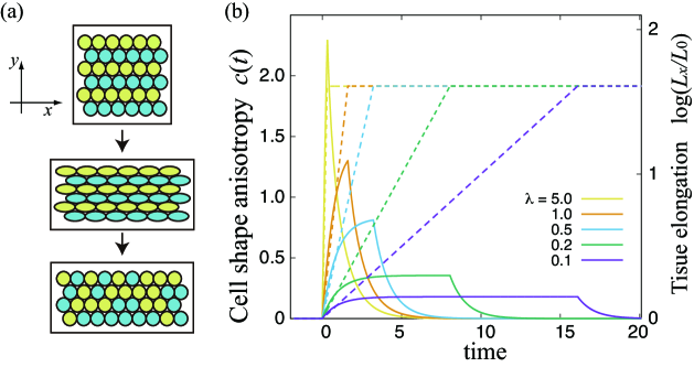
Figure 3: Passive relaxation of cellular shape anisotropy following the tissue stretching. (a) Stretching along the $x$-axis of a tissue with the constant area. Cells are elongated, and after relaxation, they recover their circular shapes. (b) Cellular shape anisotropy $c(t)$ (solid lines). Forced deformation ($a=5$, dashed lines) with the deformation rates $\lambda=5.0,1.0,0.5,0.2,0.1\,\times 10^{-4}\,\mathrm{s}^{-1}$ is followed by relaxation (numerical solution of (18)). Parameters are $\gamma_{0}/(4M_{0})^{1/2}=0.1\,\mathrm{mN}\,\mathrm{m}^{-1}$ , $2\pi\kappa_{0}=0.4\,\mathrm{mN}\,\mathrm{m}^{-1}$, $\nu_{1}=0.1$, and $\eta_{1}=1.0\,\mathrm{Pa}\,\mathrm{m}\,\mathrm{s}$. The characteristic time $\tau_{\mathrm{r}}=\eta_{1}/2\Gamma(0)=1.0\times 10^{4}\,\mathrm{s}$ is used as the time unit.

Figure 4: Active contraction-elongation (CE) of a tissue. (a) Schematics of CE in Xenopus embryo Tada2012 ; Shindo2014 . Due to the cell rearrangement, the tissue simultaneously shrinks along the medio-lateral, $y$ axis and elongates along the anterior-posterior, $x$-axis, whereas the cells adopt an elongated shape along the $y$-axis. (b) Phase diagram showing the dependence of the cellular shape anisotropy $c$ and the tissue deformation rate $\partial_{x}v_{x}$ on the active parameters $\zeta_{\mathrm{Q}}\,\Delta\mu$ and $\beta_{\mathrm{Q}}\,\Delta\mu$. Ellipses illustrate cellular shape, and arrows point to the direction of tissue flow. Parameter values are set as $\nu_{1}=0.1~{}<\!1$, $\eta_{1}=1.0\,\mathrm{Pa}\,\mathrm{m}\,\mathrm{s}$, and $\eta=5.0\,\mathrm{Pa}\,\mathrm{m}\,\mathrm{s}$.

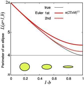
Fig. S​​ 1: Euler approximation of the perimeter $L$ of an ellipse of semi-axes $a=1$ and $b\in[0,1]$ as a function of $1-b$ at first and second order is compared to the exact value. The isotropic case corresponds to $a=b$, or $1-b=0$.

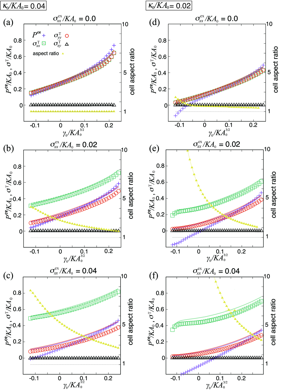
Fig. S​​ 2: Macroscopic stress expressions calculated from coarse-grained cell shape tensor $M$ (symbols) are compared with the true ones (solid lines) obtained by CVM simulations (left vertical axis), as a function of the non-dimensionalized parameter $\gamma_{0}/KA_{0}^{3/2}$, with $\kappa_{0}/KA_{0}=0.02$ (right column) and $\kappa_{0}/KA_{0}=0.04$ (left column). $P^{\mathrm{ce}}$ and $\sigma^{\mathrm{T}}$ are the pressure and stresses originating from cell elasticity and cell junction tensions, respectively. Yellow triangles denote the mean cell shape aspect ratio (right vertical axis), equal to $\exp(2c)$ in terms of the cell shape anisotropy. Components of the external stress are set as $\sigma^{\mathrm{ex}}_{xy}=\sigma^{\mathrm{ex}}_{yy}=0$, with (from left to right column) $\sigma^{\mathrm{ex}}_{xx}=0.0$, $0.02$, $0.04$.

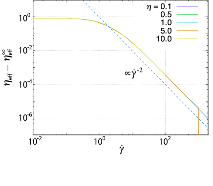
Fig. S​​ 3: Log-log plot of the difference $\eta_{\mathrm{eff}}-\eta_{\mathrm{eff}}^{\infty}$ as a function of the shear rate $\dot{\gamma}$. The dashed line corresponds to $\eta_{\mathrm{eff}}-\eta_{\mathrm{eff}}^{\infty}\propto\dot{\gamma}^{-2}$.

References

- (1) Heisenberg CP, Bellaïche Y (2013) Forces in tissue morphogenesis and patterning. Cell 153(5):948-962.
- (2) Sampathkumar A, Yan A, Krupinski P, Meyerowitz EM (2014) Physical forces regulate plant development and morphogenesis. Curr Biol 24(10):R475-R483.
- (3) Lecuit T, Lenne PF, Munro E (2011) Force generation, transmission, and integration during cell and tissue morphogenesis. Annu Rev Cell Dev Biol 27:157-184.
- (4) Blanchard GB, Adams RJ (2011) Measuring the multi-scale integration of mechanical forces during morphogenesis. Curr Opin Genet Dev 21:653-663.
- (5) Aigouy B, et al. (2010) Cell flow reorients the axis of planar polarity in the wing epithelium of Drosophila. Cell 142:773-86.
- (6) Sugimura K, Ishihara S (2013) The mechanical anisotropy in a tissue promotes ordering in hexagonal cell packing. Development 140(19):4091-4101.
- (7) Aw WY, Heck BW, Joyce B, Devenport D (2016) Transient tissue-scale deformation coordinates alignment of planar cell polarity junctions in the mammalian skin. Curr Biol 26(16):2090-2100.
- (8) Uyttewaal M, et al. (2012) Mechanical stress acts via Katanin to amplify differences in growth rate between adjacent cells in Arabidopsis. Cell 149(2):439-451.
- (9) Schluck T, Nienhaus U, Aegerter-Wilmsen T, Aegerter CM (2013) Mechanical control of organ size in the development of the Drosophila wing disc. PLoS One 8(10):e76171.
- (10) Wyatt TP, et al. (2015) Emergence of homeostatic epithelial packing and stress dissipation through divisions oriented along the long cell axis. Proc Nat Acad Sci USA 112(18):5726-5731.
- (11) Bosveld F, et al. (2012) Mechanical control of morphogenesis by Fat/Dachsous/Four-jointed planar cell polarity pathway. Science 336:724-727.
- (12) Guirao B, et al. (2015) Unified quantitative characterization of epithelial tissue development. eLife 4:e08519.
- (13) Ishihara S, Sugimura K (2012) Bayesian inference of force dynamics during morphogenesis. J Theor Biol 313:201-211.
- (14) Ishihara S, et al. (2013) Comparative study of non-invasive force and stress inference methods in tissue. Eur Phys J E Soft Matter 36:45.
- (15) Chiou KK, Hufnagel L, Shraiman BI (2012) Mechanical stress inference for two dimensional cell arrays. PLoS Comput Biol 8(5):e1002512.
- (16) Brodland GW, et al. (2014) CellFIT: A cellular force-inference toolkit using curvilinear cell boundaries. PLoS One 9(6):e99116.
- (17) Khalilgharibi N, Fouchard J, Recho P, Charras G, Kabla A (2016) The dynamic mechanical properties of cellularised aggregates. Curr Opin Cell Biol 42:113-120.
- (18) Honda H (1983) Geometrical models for cells in tissues. Int Rev Cytol 81:191-248.
- (19) Graner F, Sawada Y (1993) Can surface adhesion drive cell rearrangement? part II: A geometrical model. J Theor Biol 164:477-506.
- (20) Fletcher AG, Osterfield M, Baker RE, Shvartsman SY (2014) Vertex models of epithelial morphogenesis. Biophys J 106(11):2291-2304.
- (21) Marée AFM, Grieneisen VA, Hogeweg P (2007) The cellular Potts model and biophysical properties of cells, tissues and morphogenesis Single-Cell-Based Models in Biology and Medicine, eds Anderson ARA, Chaplain MAJ, Rejniak KA (Springer-Verlag, New York).
- (22) Brodland GW (2004) Computational modeling of cell sorting, tissue engulfment, and related phenomena: A review. Appl Mech Rev 57:47-76.
- (23) Fung YC (1993) Biomechanics mechanical properties of living tissues 2nd ed. (Springer-Verlag, New York).
- (24) Tlili S, et al. (2015) Mechanical formalisms for tissue dynamics. Eur Phys J E Soft Matter 38:121.
- (25) Shraiman BI (2005) Mechanical feedback as a possible regulator of tissue growth. Proc Nat Acad Sci USA 102:3318-3323.
- (26) Ranft J, et al. (2010) Fluidization of tissues by cell division and apoptosis. Proc Nat Acad Sci USA 107:20863-20868.
- (27) Popović M, et al. (2017) Active dynamics of tissue shear flow. New J Phys 19:033006.
- (28) Brodland GW, Chen DIL, Veldhuis JH (2006) A cell-based constitutive model for embryonic epithelia and other planar aggregates of biological cells. Int. J. Plast. 22, 965-995.
- (29) Murisic N, Hakim V, Kevrekidis IG, Shvartsman SY, Audoly B (2015) From discrete to continuum models of three-dimensional deformations in epithelial sheets. Biophys J 109:154-163.
- (30) Turner S (2005) Using cell potential energy to model the dynamics of adhesive biological cells. Phys Rev E 71:041903.
- (31) Fozard JA, Byrne HM, Jensen OE, King JR (2010) Continuum approximations of individual-based models for epithelial monolayers. Math Med Biol 27:39-74.
- (32) Larson RG (1988) Constitutitive Equations for Polymer Melts and Solutions (Butterworth-Heinemann).
- (33) Leonov AI (1976) Nonequilibrium thermodynamics and rheology of viscoelastic polymer media. Rheologica Acta 15:85-98.
- (34) Leonov AI (1987) On a class of constitutive equations for viscoelastic liquids. J Non-Newtonian Fluid Mech 25:1-59.
- (35) Marmottant P, Raufaste C, Graner F (2008) Discrete rearranging disordered patterns, part II: 2D plasticity, elasticity and flow of a foam. Eur Phys J E 25:371-384.
- (36) Bénito S, Bruneau CH, Colin T, Gay C, Molino F (2008) An elasto-visco-plastic model for immortal foams or emulsions. Eur Phys J E 25:225-251.
- (37) Larson RG (1983) Convection and diffusion of polymer network. J Non-Newtonian Fluid Mech 13:279-308.
- (38) Farhadifar R, Röper JC, Aigouy B, Eaton S, Jülicher F (2007) The influence of cell mechanics, cell-cell interactions, and proliferation on epithelial packing. Curr Biol 17:2095-2104.
- (39) Chandrupatla TR (2010) The perimeter of an ellipse. Math Scientist 35:122-131.
- (40) Batchelor GK (1970) The stress system in a suspension of force-free particles. J Fluid Mech 41:545-570.
- (41) Merkel M, et al (2017) Triangles bridge the scales: Quantifying cellular contributions to tissue deformation. Phys Rev E 95:032401.
- (42) Staple DB, et al. (2010) Mechanics and remodelling of cell packings in epithelia. Eur Phys J E 33:117-127.
- (43) De Groot SR, Mazur P (1962) Non-equilibrium thermodynamics (North-Holland Publishing Company, Amsterdam).
- (44) Etournay R, et al. (2015) Interplay of cell dynamics and epithelial tension during morphogenesis of the drosophila pupal wing. eLife 4:e14334.
- (45) Sato K, et al. (2015) Left-right asymmetric cell intercalation drives directional collective cell movement in epithelial morphogenesis. Nat Comm 6:10074.
- (46) Saw TB, et al. (2017) Topological defects in epithelia govern cell death and extrusion. Nature. 544:212-216
- (47) Kruse K, Joanny JF, Jülicher F, Prost J, Sekimoto K (2005) Generic theory of active polar gels: a paradigm for cytoskeletal dynamics. Eur Phys J E 16:5-16.
- (48) Marchetti MC, et al. (2013) Hydrodynamics of soft active matter. Rev Mod Phys 85:1143.
- (49) Bambardekar K, Clément R, Blanc O, Chardès C, Lenne PF (2015) Direct laser manipulation reveals the mechanics of cell contacts in vivo. Proc Nat Acad Sci USA 112:1416-1421.
- (50) Guevorkian K, Colbert MJ, Durth M, Dufour S, Brochard-Wyart F (2010) Aspiration of biological viscoelastic drops. Phys Rev Lett 104:218101.
- (51) Stirbat TV, et al. (2013) Fine tuning of tissues’ viscosity and surface tension through contractility suggests a new role for -catenin. PLoS One 8:e52554.
- (52) Tada M, Heisenberg CP (2012) Convergent extension: using collective cell migration and cell intercalation to shape embryos. Development 139:3897-3904.
- (53) Shindo A, Wallingford JB (2014) PCP and septins compartmentalize cortical actomyosin to direct collective cell movement. Science 343:649-652.
- (54) Rozbicki E, et al. (2015) Myosin-II-mediated cell shape changes and cell intercalation contribute to primitive streak formation. Nat Cell Biol 17:397-408.
- (55) Morishita Y, Hironaka K, Lee S, Jin T, Ohtsuka D (2017) Reconstructing 3D deformation dynamics for curved epithelial sheet morphogenesis from positional data of sparsely-labelled cells. Nat Commun In press.
- (56) Zajac M, Jones GL, Glazier JA (2000) Model of convergent extension in animal morphogenesis. Phys Rev Lett 85(9):2022-2025.
- (57) Zajac M, Jones GL, Glazier JA (2003) Simulating convergent extension by way of anisotropic differential adhesion. J Theor Biol 222:247-259.
- (58) Oswald P (2009) Rheophysics: The Deformation and Flow of Matter (Cambridge University Press, UK).
- (59) Marmottant P, et al. (2009) The role of fluctuations and stress on the effective viscosity of cell aggregates. Proc Nat Acad Sci USA 106:17271-17275.
- (60) Blanchard GB, et al. (2009) Tissue tectonics: morphogenetic strain rates, cell shape change and intercalation. Nat Methods 6:458-464.
- (61) G. B. Blanchard (2017) Taking the strain: quantifying the contributions of all cell behaviours to changes in epithelial shape. Phil Trans Roy Soc B 372:20150513.
- (62) Yabunaka S, Marcq P, Preprint (2017).
- (63) Kabla AJ (2012) Collective cell migration: leadership, invasion and segregation. J R Soc Interface 9:3268-3278.
- (64) Barton DL, Henkes S, Weijer CJ, Sknepnek R (2016) Active vertex model for cell-resolution description of epithelial tissue mechanics. BioRXiV doi: https://doi.org/10.1101/095133.

References

- (1) S. Tlili, C. Gay, F. Graner, P. Marcq, F. Molino, and P. Saramito, Mechanical formalisms for tissue dynamics. Eur. Phys. J. E 38, 33 (2015).
- (2) R. Farhadifar, J. C. Röper, B. Aigouy, S. Eaton, and F. Jülicher, The influence of cell mechanics, cell-cell interactions, and proliferation on epithelial packing. Curr. Biol. 17, 2095 (2007).
- (3) A. G. Fletcher, M. Osterfield, R. E. Baker and S. Y. Shvartsman, Vertex models of epithelial morphogenesis. Biophys. J. 106, 2291 (2014).
- (4) S. Ishihara and K. Sugimura, Bayesian inference of force dynamics during morphogenesis. J. Theor. Biol. 313, 201 (2012).
- (5) S. Ishihara, K. Sugimura, S. J. Cox, I, Bonnet, Y. Bellaïche, and F. Graner, Comparative study of non-invasive force and stress inference methods in tissue. Eur. Phys. J. E 36, 45 (2013).
- (6) B. Guirao, S. U. Rigaud, F. Bosveld, A. Bailles, J. Lopez-Gay, S. Ishihara, K. Sugimura, F. Graner, and Y. Bellaïche, Unified quantitative characterization of epithelial tissue development. eLife 4, e08519 (2015).
- (7) C. Steger, On the Calculation of Arbitrary Moments of Polygons. Technical Report FGBV-96-05, Technische Universität München (1996)
- (8) T. R. Chandrupatla, The perimeter of an ellipse. Math. Scientist 35, 122 (2010).
- (9) K. Sato, T. Hiraiwa, E. Maekawa, A. Isomura, T. Shibata and E. Kuranaga, Left-right asymmetric cell intercalation drives directional collective cell movement in epithelial morphogenesis. Nat. Comm. 6, 10074 (2015).