On Affine Invariant $L_{p}$ Depth Classifiers based
on an Adaptive Choice of $p$

Subhajit Dutta and Anil K. Ghosh

Abstract

In this article, we use L_p depth for classification of multivariate data, where the value of $p$ is chosen adaptively using observations from the training sample. While many depth based classifiers are constructed assuming elliptic symmetry of the underlying distributions, our proposed L_p depth classifiers cater to a larger class of distributions. We establish Bayes risk consistency of these proposed classifiers under appropriate regularity conditions. Several simulated and benchmark data sets are analyzed to compare their finite sample performance with some existing parametric and nonparametric classifiers including those based on other notions of data depth.

Key words: Bayes risk, Data depth, Kernel density estimation, $l_{p}$-symmetric distributions, Maximum likelihood estimation, Misclassification rates.

Short title: Affine invariant $L_{p}$ depth classifiers

1 Introduction

Data depth measures the centrality of a point x in $\mathbb{R}^{d}$ with respect to a $d$-dimensional data cloud, or a $d$-dimensional probability distribution. As a result, it provides a centre-outward ordering of multivariate data. Various notions of data depth are available in the literature (see, e.g., Liu, Parelius and Singh, 1999; Zuo and Serfling, 2000), and they have been used for generalizing many univariate statistical methods to the multivariate setup. One important application is supervised classification. Ghosh and Chaudhuri (2005) introduced maximum depth classifiers and also developed a modified classifier based on Tukey’s (1975) half-space depth (HD). Later, Dutta and Ghosh (2012) investigated some robust classifiers based on projection depth (PD) (see, e.g., Zuo and Serfling, 2000) and robust versions of Mahalanobis depth (MD). Li, Cuesta-Albertos and Liu (2012) developed nonparametric classifiers based on depth-depth (DD) plots. Other depth based classification methods include the work of Jörnsten (2004), Hoberg and Mosler (2006), Hartikainen and Oja (2006), Cui, Lin and Yang (2008) and Paindaveine and Van Bever (2015).

Constructions of most of these classifiers were motivated by elliptic symmetry (i.e., $l_{2}$-symmetry after an affine transformation; see, e.g., Fang, Kotz and Ng, 1989) of the competing class distributions. In this article, we develop some classifiers motivated by general $l_{p}$-symmetry (after an affine transformation) of the underlying distributions. We assume that the density of each competing class to be continuous, and of the form $f(\mbox{\bf x})=\psi(\|{\bf A}(\mbox{\bf x}-{\bf b})\|_{p})$, where $p\geq 1$, ${\bf b}$ is a $d$-dimensional vector, ${\bf A}$ is a $d\times d$ non-singular matrix and $\psi:\mathbb{R}_{+}\rightarrow\mathbb{R}_{+}$ is a scalar continuous function. Here, $\|\mbox{\bf z}\|_{p}=(|z_{1}|^{p}+\cdots+|z_{d}|^{p})^{1/p}$ for any $\mbox{\bf z}=(z_{1},\ldots,z_{d})^{T}\in\mathbb{R}^{d}$. Clearly, the location (i.e., the centre of symmetry) $\mu$ of this distribution is ${\bf b}$. In the case of $p=2$ (i.e., elliptic symmetry), the associated scatter matrix $\Sigma$ is given by $({\bf AA}^{T})^{-1}$. If $f$ is assumed to have finite second moments, it has the mean vector $E[\mbox{\bf X}]={\bf b}$ and the dispersion matrix $E[(\mbox{\bf X}-\mbox{\boldmath$\mu$})(\mbox{\bf X}-\mbox{\boldmath$\mu$})^{T}]=c_{p,\psi}~{}{({\bf AA}^{T})}^{-1}$, where $c_{p,\psi}$ is a positive constant that depends on $p$ and $\psi$. So, ${\bf A}$ can be viewed as a square root of $\mbox{\boldmath$\Sigma$}^{-1}$ (upto a scalar constant). Several authors have studied various properties of multivariate $l_{p}$-symmetric distributions (see, e.g., Yue and Ma, 1995; Gupta and Song, 1997). Sinz and Bethge (2010) used $l_{p}$-symmetric distributions to develop various statistical tools including independent component analysis. Arellano-Valle and Richter (2012) have introduced skewed versions of $l_{p}$-symmetric distributions. Throughout this article, by $l_{p}$-symmetric, we mean $l_{p}$-symmetric after applying an affine transformation (as we have discussed above).

If the underlying class distributions are $l_{2}$-symmetric (i.e., spherically or elliptically symmetric), for several existing notions of data depth, the class densities turn out to be functions of depths. Consequently, the Bayes classifier can be expressed as a function of data depths corresponding to different competing classes. This is the main argument used in proving the Bayes risk consistency for most of the existing depth based classifiers. However, if the depth contours fail to match the density contours, one cannot use such mathematical arguments. To appreciate this, consider a two-class problem with equal priors and class densities $f_{1}(\mbox{\bf x})=c_{p}\exp(-\|\mbox{\bf x}\|_{p}^{p})$ and $f_{2}(\mbox{\bf x})=c_{p}/\sigma^{d}\exp(-\|\mbox{\bf x}\|_{p}^{p}/\sigma)$, where $\sigma\neq 1$ is a positive constant, and $c_{p}$ is the normalizing constant. Clearly, the boundary of the Bayes classifier is of the form $\{\mbox{\bf x}:\|\mbox{\bf x}\|_{p}=K_{0}\}$ for some $K_{0}>0$. Now, MD contours for each class are concentric hyper-spheres of the form $\{\mbox{\bf x}:\|\mbox{\bf x}\|_{2}=K\}$ for varying choices of $K>0$. Therefore, when $p\neq 2$, no classifier based on MD can yield the Bayes class boundary.

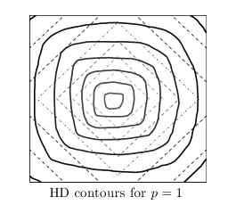
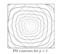
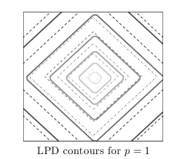
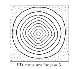
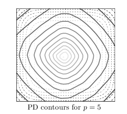
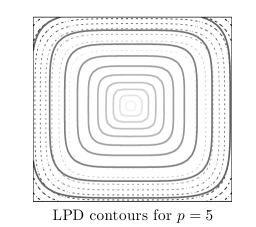
Figure 1: Density contours (dotted curves) of $l_{p}$ symmetric distributions for $p=1$ and $p=5$, and the corresponding HD, PD and L_pD contours (bold curves) estimated from the data.

For $l_{p}$-symmetric distributions with $p\neq 2$, Dutta, Ghosh and Chaudhuri (2011) proved that the density cannot be a function of HD as well. Figure 1 shows HD and PD contours (indicated using bold curves) computed based on 2000 observations from two $l_{p}$-symmetric densities (density contours are shown using dotted curves) with $p=1$ and $p=5$ (see the left and the middle panels). This figure clearly shows that the class density cannot be a function of depth in either of these cases.

To overcome this limitation, we use L_p depth (see, e.g., Zuo and Serfling, 2000) with a data driven choice of $p$. L_p depth (L_pD) of an observation x with respect to a multivariate distribution function $F$ is defined as $\delta_{p}(\mbox{\bf x})=[1+r_{p}(\mbox{\bf x})]^{-1}$, where $r_{p}(\mbox{\bf x})=\|\mbox{\boldmath$\Sigma$}^{-1/2}(\mbox{\bf x}-\mbox{\boldmath$\mu$})\|_{p}$ with $\mu$ and $\Sigma$ being the location and the scatter associated with $F$. The empirical version of $\delta_{p}(\mbox{\bf x})$ is obtained by estimating $p$, and $r_{p}(\mbox{\bf x})$ from the data (see Section 2 for details). The right panel of Figure 1 shows that the empirical L_pD contours based on 2000 observations almost coincide with the underlying $l_{p}$-symmetric density contours both for $p=1$ and $p=5$. So, classifiers based on $\delta_{p}(\mbox{\bf x})$ are expected to yield an improved performance.

2 Estimation of L_p Depth

To construct a classifier based on $\delta_{p}(\mbox{\bf x})$, first one needs to find an appropriate value of $p$ for each of the competing classes. We choose the value of $p$ which fits to the data well. Suppose $\mbox{\bf x}_{1},\mbox{\bf x}_{2},\ldots,\mbox{\bf x}_{n}$ are $n$ independent observations from a $l_{p}$-symmetric distribution with density $f$. If ${\bf b}$ and ${\bf A}$ denote the associated location and scatter parameters (defined in Section 1), then $f$ can be expressed as:

$$f(\mbox{\bf x},p)=|{\bf A}|~{}\frac{p^{d-1}\Gamma(d/p)}{2^{d}[\Gamma(1/p)]^{d}}\frac{g_{p}(\delta_{p}(\mbox{\bf x}))~{}\delta_{p}(\mbox{\bf x})^{d+1}}{{[1-\delta_{p}(\mbox{\bf x})]}^{d-1}},$$

where $\delta_{p}(\mbox{\bf x})=[1+\|{\bf A}(\mbox{\bf x}-{\bf b})\|_{p}]^{-1}$, and $g_{p}$ is the density of $\delta_{p}(\mbox{\bf X})$ (see Lemma 1 in the Appendix). In Section 2.1, we discuss the estimation procedure for $p$, assuming that ${\hat{\bf b}}$ and ${\hat{\bf A}}$ (estimates for ${\bf b}$ and ${\bf A}$, respectively) are given. In Section 2.2, we construct ${\hat{\bf b}}$ and ${\hat{\bf A}}$ which makes the estimate of $p$, and hence the empirical version of L_pD affine invariant.

2.1 Estimation of $p$

For any fixed $p$, using the data $\mbox{\bf x}_{1},\mbox{\bf x}_{2},\ldots,\mbox{\bf x}_{n}$ from $f$, we first compute $\hat{r_{p}}(\mbox{\bf x}_{i})=\|{\hat{\bf A}}(\mbox{\bf x}_{i}-{\hat{\bf b}})\|_{p}$ and ${\hat{\delta}}_{p}(\mbox{\bf x}_{i})=[1+\hat{r_{p}}(\mbox{\bf x}_{i})]^{-1}$ for $i=1,2,\ldots,n$. In order to estimate $f$, one needs an estimate of $g_{p}$. Assuming $\hat{\delta_{p}}(\mbox{\bf x}_{1}),\ldots,\hat{\delta_{p}}(\mbox{\bf x}_{n})$ as sample observations, we estimate it using the kernel density estimation (see, e.g., Silverman, 1998) method. This density estimate is given by $\hat{g}_{p,h}(\delta)=\frac{1}{nh}\sum_{i=1}^{n}K\left[h^{-1}({\delta-\hat{\delta_{p}}(\mbox{\bf x}_{i})})\right]$, where $K$ is the kernel function and $h$ is the associated bandwidth parameter. We use the Gaussian kernel $K(t)=(2\pi)^{-1/2}e^{-t^{2}/2}$, and $h$ is chosen using the bandwidth selection method proposed in Sheather and Jones (1991). So, under the assumption of $l_{p}$ symmetry, the estimate of the density function $f$ is given by

$$\hat{f}_{h}(\mbox{\bf x},p)=|\hat{{\bf A}|}~{}\frac{p^{d-1}\Gamma(d/p)}{2^{d}\{\Gamma(1/p)\}^{d}}\frac{\hat{g}_{p,h}(\hat{\delta_{p}}(\mbox{\bf x}))~{}\hat{\delta_{p}}(\mbox{\bf x})^{d+1}}{[1-\hat{\delta}_{p}(\mbox{\bf x})]^{d-1}}.$$

Irrespective of the dimension of the data, here we need only one-dimensional kernel density estimation. Similar approaches for depth based density estimation were also used by Fraiman, Liu and Mechole (1997) and Hartikainen and Oja (2006).

We compute the estimated joint likelihood ${\cal L}_{p}(\mbox{\bf x}_{1},\ldots,\mbox{\bf x}_{n})$ $=\prod_{i=1}^{n}\hat{f}_{h}(\mbox{\bf x}_{i},$ $p)$ for different $p$, and choose the one that maximizes ${\cal L}_{p}(\mbox{\bf x}_{1},\ldots,\mbox{\bf x}_{n})$ or $\log{\cal L}_{p}(\mbox{\bf x}_{1},\ldots,$ $\mbox{\bf x}_{n})$. However, note that if $\hat{\delta}_{p}(\mbox{\bf x})$ is close to zero or unity, $|\log\hat{f}_{h}(\mbox{\bf x},p)|$ tends to be very influential. So, we consider only those $\mbox{\bf x}_{i}$s for which $\hat{\delta}_{p}(\mbox{\bf x}_{i})$ lie between $\zeta_{1n}$ and $\zeta_{2n}$ ($0<\zeta_{1n}<\zeta_{2n}<1$) and find $\hat{p}$ (the estimate of $p$) by maximizing

$${\varphi}_{p}(\mbox{\bf x}_{1},\cdots,\mbox{\bf x}_{n})=\sum_{\{i~{}:~{}\hat{\delta}_{p}(\mbox{\bf x}_{i})\in[\zeta_{1n},\zeta_{2n}]\}}\log\hat{f}_{h}(\mbox{\bf x}_{i},p)$$

over ${\cal P}=\{p_{1},p_{2},\ldots,p_{M}\}$, a finite set of values for $p$. The following theorem suggests a suitable choice for $[\zeta_{1n},\zeta_{2n}]$, and gives the asymptotic behavior of $\hat{p}$ under appropriate regularity conditions.

Theorem 1: Let $\mbox{\bf X}_{1},\mbox{\bf X}_{2},\ldots,\mbox{\bf X}_{n}$ be independent and identically distributed with the density of the form $f(\mbox{\bf x},p_{0})=\psi_{0}(\|{\bf A}(\mbox{\bf x}-{\bf b})\|_{p_{0}})$ for some $p_{0}\geq 1$. For any $p\geq 1$, define $\zeta_{1n}=\zeta_{1}(p)$ and $\zeta_{2n}=\zeta_{2}(p)$ as the $\alpha_{1n}$-th and $\alpha_{2n}$-th quantile of $g_{p}$, where $\alpha_{1n}\downarrow 0$, $\alpha_{2n}\uparrow 1$ and $n^{1/2}~{}\min\{\zeta_{1n},1-\zeta_{2n}\}\rightarrow\infty$ as $n\rightarrow\infty$. Now, consider the following assumptions:

(C1) ${\hat{\bf A}}$ and ${\hat{\bf b}}$ are $\sqrt{n}$-consistent estimates of $a_{0}{\bf A}$ and ${\bf b}$ (i.e., $\sqrt{n}\|{\hat{\bf A}}-a_{0}A\|_{F}=O_{P}(1)$, where $a_{0}>0$ and $\|\cdot\|_{F}$ denotes the Frobenious norm; and $\sqrt{n}\|{\hat{\bf b}}-{\bf b}\|_{p}=O_{P}(1)$ for any $p\geq 1)$, respectively.

(C2) For any $p\geq 1$, $g_{p}$ is absolutely continuous and the bandwidth $h$ associated with the estimation of $g_{p}$ is of the order $O(n^{-1/4+\varepsilon})$ for some $\varepsilon\in(0,1/4)$.

(C3) For any $p\geq 1$, $\displaystyle n^{1/2}h^{2}\inf_{\{\delta_{p}(\mbox{\bf x})\in~{}[\zeta_{1n},\zeta_{2n}]\}}g_{p}(\delta_{p}(\mbox{\bf x}))\rightarrow\infty$ as $n\rightarrow\infty$.

Assume (C1)-(C3), and define $\hat{p}_{n}=\arg\max_{p}{\varphi}_{p}(\mbox{\bf X}_{1},\cdots,\mbox{\bf X}_{n})$. If $p_{0}\in{\cal P}$, then $\hat{p}_{n}\stackrel{{\scriptstyle P}}{{\rightarrow}}p_{0}$ as $n\rightarrow\infty$. If $p_{0}\notin{\cal P}$, then $\hat{p}_{n}\stackrel{{\scriptstyle P}}{{\rightarrow}}p_{0}^{*}$, where $p_{0}^{*}$ minimizes the Kullback-Leibler divergence between $f(\cdot,p_{0})$ and $f(\cdot,p)$ over $p\in{\cal P}$.

If $g_{p}$ is bounded away from zero and infinity, it is easy to see that $(C3)$ holds for any choice of $\alpha_{1n}$ and $\alpha_{2n}$. In fact, $(C3)$ holds if $g_{p}$ remains bounded away from zero on any bounded interval inside its support. Also note that the Sheather-Jones bandwidth (see Sheather and Jones, 1991) that we use for kernel density estimation is of the order $O_{P}(n^{-1/5})$.

The quantities ${\hat{\bf b}}$ and ${\hat{\bf A}}$ can be obtained directly from ${\hat{}\mbox{\boldmath$\mu$}}$ and ${\hat{}\mbox{\boldmath$\Sigma$}}$, the estimates of $\mu$ and $\Sigma$. Affine equivariant estimates of $\mu$ and $\Sigma$ (e.g., usual moment based estimates or minimum covariance determinant (MCD) estimates) can be used for this purpose. Assuming the existence of second order moments, the sample mean converges to $\mu$ and the sample dispersion matrix converges to constant multiple of $\Sigma$ at $\sqrt{n}$ rate as stated in $(C1)$. Under appropriate regularity conditions, we have $\sqrt{n}$ convergence for MCD estimates as well (see Cator and Lopuhaä, 2012).

2.2 Estimation of ${\bf b}$ and ${\bf A}$

We can continue to use ${\hat{}\mbox{\boldmath$\mu$}}$ (the moment based estimate, or the MCD estimate) as an estimate of ${\bf b}$. However, to construct ${\hat{\bf A}}$, one has to compute the square root of ${\hat{}\mbox{\boldmath$\Sigma$}}$. Note that the symmetric square root of ${\hat{}\mbox{\boldmath$\Sigma$}}$ is not affine eqivariant. We construct an affine equivariant square root of ${\hat{}\mbox{\boldmath$\Sigma$}}$ using the transformation re-transformation technique (see, e.g., Chakraborty and Chaudhuri, 1996). Consider a subset $\alpha=\{i_{1},i_{2},\ldots,i_{d+1}\}$ of the set $\{1,2,\ldots,n\}$. Use it to construct a $d\times d$ matrix ${\mathbb{X}}(\alpha)=[(\mbox{\bf x}_{i_{1}}-\mbox{\bf x}_{i_{d+1}})~{}(\mbox{\bf x}_{i_{2}}-\mbox{\bf x}_{i_{d+1}})~{}\ldots~{}(\mbox{\bf x}_{i_{d}}-\mbox{\bf x}_{i_{d+1}})]$, and compute ${\mathbb{Z}}(\alpha)={\mathbb{X}}{(\alpha)}^{T}{\hat{}\mbox{\boldmath$\Sigma$}}^{-1}~{}{\mathbb{X}}{(\alpha)}$. Now, find an $\alpha_{0}$ that makes ${\mathbb{Z}}(\alpha)$ close to a constant multiple of ${\bf I}_{d}$ (the $d\times d$ identity matrix). For practical purposes, one may choose an $\alpha_{0}$ that maximizes the ratio of the determinant of ${\mathbb{Z}}(\alpha)$ to the trace of ${\mathbb{Z}}(\alpha)$. However, finding the actual maximizer $\alpha_{0}$ is computationally difficult. So, following Chakraborty and Chaudhuri (1996), we choose an $\alpha$ which makes the ratio is close to $1$ ($\geq 0.99$).

Figure 2: Density contours (dotted curves) and estimated L_pD contours (bold curves).

The matrix ${\mathbb{X}}(\alpha_{0})$ can now be considered as a square root of ${\hat{}\mbox{\boldmath$\Sigma$}}$ (upto a scalar multiple). The use of ${\hat{\bf A}}={\mathbb{X}}^{-1}(\alpha_{0})$ makes $\hat{\delta}_{p}(\mbox{\bf x})$ affine invariant. To study the empirical performance of this estimation method, we generated 400 observations from the density $f_{1}(x_{1},x_{2})\propto\exp\{-(|x_{1}|+{|x_{2}|}/{0.3})\}$ (which is $l_{1}$-symmetric), and then rotated them by an angle of $3\pi/4$. The left panel in Figure 2 shows that the estimated L_pD contours (solid curves) closely matches the corresponding density contours (dotted curves). We carried out a second experiment with observations from the density $f_{2}(x_{1},x_{2})\propto\exp\{-(|x_{1}|^{5}+{|x_{2}|^{5}}/{0.3})\}$ (which is $l_{5}$-symmetric), which were further rotated by an angle of $\pi/4$. In this example also, the estimation method worked quite well (see the right panel in Figure 2).

3 Classification with L_p Depth

In this section, we first study the maximum L_pD classifier. This classifier works well when the competing classes have the same prior, and they differ only in their locations. However, if the classes have unequal priors and/or they differ only in their scatters and shapes, the maximum depth classifier may fail to have satisfactory performance. To cope with such cases, we develop a modified classifier in Section 3.2.

3.1 Maximum L_p depth classifier

The maximum L_pD classifier classifies an observation to the class with respect to which it has the maximum depth. To construct the empirical version of L_pD, we estimate $p$ and $\delta_{p}(\mbox{\bf x})$ from the data (as discussed in Section 2). Suppose there are $J$ competing classes with densities $f_{1},\ldots,f_{J}$, and for the $j$-th class, these estimates are denoted by $\hat{p}_{j}$ and ${\hat{\delta}}_{\hat{p}_{j},j}(\mbox{\bf x})$, respectively, for $1\leq j\leq J$. Then, the maximum L_pD classifier classifies an observation x to the $j$-th class if ${\hat{\delta}}_{\hat{p}_{j},j}(\mbox{\bf x})>{\hat{\delta}}_{\hat{p}_{i},i}(\mbox{\bf x})$ for all $i\neq j$. However, this classifier is mainly used when the competing classes differ only in their locations, and in such cases it is more appealing to use a common value of $p$ for all classes. If $\mbox{\bf x}_{j1},\mbox{\bf x}_{j2},\ldots,\mbox{\bf x}_{jn_{j}}$ are observations from the $j$-th ($1\leq j\leq J$) class, this common value of $p$ can be estimated by maximizing the joint log-likelihood function $\sum_{j=1}^{J}\varphi_{p}(\mbox{\bf x}_{j1},\mbox{\bf x}_{j2},\ldots,\mbox{\bf x}_{jn_{j}})$ over ${\cal P}$. The resulting maximum L_pD classifier is given by ${\sf d}_{1}(\mbox{\bf x})=\arg\min_{1\leq j\leq J}{\hat{\delta}}_{\hat{p},j}(\mbox{\bf x}),$ where $\hat{p}$ denotes the common estimated value of $p$.

Theorem 2: Assume the density functions $f_{1},\ldots,f_{J}$ to be unimodal, and $f_{j}$ is of the form $f_{j}(\mbox{\bf x},p_{0})=\psi(\|{\bf A}(\mbox{\bf x}-{\bf b}_{j})\|_{p_{0}})$ for some $p_{0}\in{\cal P}$ ($1\leq j\leq J$). If the prior probabilities of the competing classes are equal, under conditions $(C1)$ - $(C3)$ (stated in Theorem 1), the misclassification rate of ${\sf d}_{1}(\mbox{\bf x})$ converges to the Bayes risk as $min\{n_{1},\ldots,n_{J}\}\rightarrow\infty$.

3.2 Generalized L_p depth classifier

In practice, the prior probabilities of different classes may not be equal, and the class distributions can also differ in their scatters and shapes. In such cases, maximum depth classifiers may have higher misclassification probabilities (see, e.g., Dutta and Ghosh, 2012). We now construct the generalized L_pD classifier to cope with such situations. Suppose that there are $J$ competing classes, and $f_{h_{j}}(\mbox{\bf x},\hat{p}_{j})$ is the density estimate for the $j$-th class ($1\leq j\leq J$). In a two-class problem, this generalized L_pD classifier is given by

$${\sf d}_{2}(\mbox{\bf x})=\left\{\begin{array}[]{ll}1&~{}\mbox{if}~{}~{}\hat{f}_{h_{1}}(\mbox{\bf x},\hat{p}_{1})/\hat{f}_{h_{2}}(\mbox{\bf x},\hat{p}_{2})>k,\\ 2&~{}\mbox{otherwise}.\end{array}\right.$$

where $k$ is chosen by minimizing the leave-one-out cross-validation estimate of the misclassification probability. For more than two classes, we use the pairwise classification approach followed by the method of majority voting.

Theorem 3: Suppose that for all $1\leq j\leq J$, the density $f_{j}$ is continuous, it has support over entire ${\mathbb{R}}^{d}$ and is of the form $f(\mbox{\bf x},p_{j}^{\circ})=\psi_{j}(\|{\bf A}_{j}(\mbox{\bf x}-{\bf b}_{j})\|_{p_{j}^{\circ}})$ for some $p_{j}^{\circ}\in{\cal P}$. Also, assume that the optimal Bayes classifier has non-empty favorable regions for each of the $J$ classes. Then, under the conditions $(C1)$ - $(C3)$ (stated in Theorem 1), the misclassification rate of the generalized L_pD classifier ${\sf d}_{2}(\mbox{\bf x})$ converges to the Bayes risk as $min\{n_{1},\ldots,n_{J}\}\rightarrow\infty$.

3.3 Comparison with other depth based classifiers

To compare the performance of our L_pD classifiers with existing classifiers based on MD, HD and PD, we carried out some simulations. To keep our examples simple, here we used two-class problems in two dimensions. For varying choices of ($p_{1},{\bf b}_{1},{\bf A}_{1}$) and ($p_{2},{\bf b}_{2},{\bf A}_{2}$), we had different types of classification problems (see Table 1). In each case, taking equal number of observations from two competing classes, we generated training and test sets of sizes 400 and 1000, respectively. Each experiment was repeated 200 times, and the average test set misclassification rates of different classifiers were computed over these 200 trials. Note that our proposed method needs ${\cal P}$ to be specified. We observed that for higher values of $p$, $l_{p}$ contours do not change much (see, e.g., Figure 1, where $l_{5}$ contours almost look like $l_{\infty}$ contours). So, throughout this article, we used ${\cal P}=\{2^{(i-1)/2};~{}i=1,2,\ldots,10\}$ for our numerical work.

Following Ghosh and Hall (2008), we computed regret functions (i.e., difference between the misclassification rate of a classifier and the Bayes risk) for different classifiers. Table 1 shows the corresponding regret ratios for classifiers based on HD, PD and MD. Regret ratio ($\eta_{t}$) of the classifier $t$ is given by ratio of the regret of that classifier and that of the L_pD classifier. Clearly, $\eta_{t}<1(>1)$ implies that the classifier is better (worse) than the L_pD classifier, and the deviation from $1$ gives an idea of how better (worse) it is. Since HD and PD classifiers are robust, here we used robust version of MD based on MCD estimates. Following Hubert and van Driessen (2004), 75% observations were used to compute these estimates. These MCD estimates were also used as ${\hat{}\mbox{\boldmath$\mu$}}$ and ${\hat{}\mbox{\boldmath$\Sigma$}}$ to compute ${\hat{\bf A}}$, ${\hat{}\mbox{\bf b}}$ and hence the empirical versions of L_p depths. For the location problems, we used maximum depth classifiers based on different notions on depth. In other examples, generalized depth based classifiers were used. In this section, we used equal prior probabilities for two competing classes.

In all these examples, L_pD classifiers outperformed the classifiers based on HD and PD. The classifiers based on HD had the worst performance in all cases, especially in location problems. The discrete nature of the empirical version of HD affected its performance, and it often had issues with ties and zero depth (also see Ghosh and Chaudhuri (2005)). As expected, the classifiers based on MD had a slight edge over the L_pD classifiers when both of the competing classes were $l_{2}$-symmetric. But, in all other cases, they were outperformed by the L_pD classifiers.

Table 1: Regret ratios of other depth-based classifiers.

Choice $\downarrow$	Difference in locations				Difference in scales				Difference in shapes
$(p_{1},{\bf b}_{1},{\bf A}_{1})$	$(p_{2},{\bf b}_{2},{\bf A}_{2})$	HD	PD	MD	$(p_{2},{\bf b}_{2},{\bf A}_{2})$	HD	PD	MD	$(p_{2},{\bf b}_{2},{\bf A}_{2})$	HD	PD	MD
$(1,{\bf 0},{\bf I}_{2})$	$(1,{\bf 1},{\bf I}_{2})$	53.01	1.54	1.26	$(1,{\bf 0},\frac{1}{9}{\bf I}_{2})$	2.59	1.13	1.01	$(2,{\bf 0},{\bf I}_{2})$	2.52	2.49	1.75
$(2,{\bf 0},{\bf I}_{2})$	$(2,{\bf 1},{\bf I}_{2})$	30.19	2.97	0.96	$(2,{\bf 0},\frac{1}{9}{\bf I}_{2})$	5.88	1.50	0.89	$(4,{\bf 0},{\bf I}_{2})$	1.57	1.40	1.14
$(8,{\bf 0},{\bf I}_{2})$	$(8,{\bf 1},{\bf I}_{2})$	25.94	6.31	1.17	$(8,{\bf 0},\frac{1}{9}{\bf I}_{2})$	5.84	3.93	2.06	$(1,{\bf 0},{\bf I}_{2})$	14.62	2.85	1.67

${\bf 0}=(0,0)^{T}$, $~{}{\bf 1}=(1,1)^{T}$, $~{}{\bf I}_{2}$ is the $2\times 2$ identity matrix.

4 Results from the Analysis of Benchmark Datasets

We analyzed eight benchmark data sets for further assessment of the generalized L_pD classifier. The hemophilia data set was taken from Johnson and Wichern (1992). All other data sets were taken either from the UCI Machine Learning Repository (http://archive.ics.uci.edu/ml/) or from the CMU Datasets Archive (http://lib.stat.cmu.edu/datasets/). Descriptions of these data sets are available at these sources. In the case of blood transfusion data set, following Li et al. (2012), we considered only one of the two linearly dependent variables for our analysis. For the synthetic data and the satellite image (satimage) data, the training and the test sets are well specified. In all other cases, we formed these sets by randomly partitioning the data in a way such that the proportion of different classes in training and test sets were as close as possible. In cases of hemophilia data and diabetes data, we used training samples of size 50 and 100, respectively. In all other cases, we divided the data set into two nearly equal halves to form the training and the test sets. In each case, this random partitioning was done 500 times. Average misclassification rates of different classifiers were computed over these 500 test sets, and they are reported in Table 3 along with their corresponding standard errors. In cases of synthetic data and satimage data, when a classifier led to a test set misclassification rate $\Delta$, its standard error was computed as $\sqrt{\Delta(1-\Delta)/n_{t}}$, for $n_{t}$ being the size of the test set.

To facilitate comparison, along with the misclassification rates of different depth based classifiers, results are also reported for two parametric classifiers (linear discriminant analysis (LDA) and quadratic discriminant analysis (QDA)) and two nonparametric classifiers (kernel discriminant analysis (KDA) and nearest neighbor classifier ($k$-NN) with the smoothing parameter chosen by the leave-one-out cross-validation method). In some of these data sets, the measurement variables were not of comparable units and scales. So, we used KDA and $k$-NN (see, e.g., Hastie, Tibshirani and Friedman, 2009; Duda, Hart and Stork, 2012) on the standardized data set, where the moment based estimate of the pooled dispersion matrix was used for standardization. Therefore, to keep our comparisons fair, instead of MCD estimates, here we used moment based estimates of location and scatter parameters for MD and L_pD classifiers as well. Since the classifier based on HD had the highest misclassification rates in almost all cases, we do not report them here. For all these benchmark data sets, sample proportions of different classes were used as their prior probabilities.

Table 2: Average misclassification rates (in %) of different classifiers and their standard errors.

Data	$d$	$J$	Train	Test	LDA	QDA	$k$-NN	KDA	PD	MD	LpD
Synthetic†	2	2	250	1000	10.80 (.98)	10.20 (.96)	11.70 (1.0)	11.00 (.99)	10.80 (.98)	10.30 (.96)	09.40 (.92)
Hemophilia	2	2	50	25	15.22 (.27)	15.47 (.26)	15.79 (.30)	15.11 (.27)	17.36 (.30)	14.33 (.29)	13.99 (.29)
Blood Tran.	3	2	374	374	22.90 (.03)	22.48 (.05)	21.39 (.06)	22.66 (.05)	22.27 (.08)	22.58 (.06)	22.41 (.07)
Diabetes	5	3	100	45	10.46 (.18)	09.39 (.18)	10.04 (.18)	11.16 (.19)	10.38 (.23)	09.23 (.17)	09.52 (.18)
Pima	8	2	384	384	23.37 (.07)	26.02 (.08)	25.73 (.08)	26.57 (.07)	29.96 (.09)	25.47 (.08)	25.34 (.08)
Vehicle	18	4	423	423	22.49 (.07)	16.38 (.07)	21.84 (.08)	21.45 (.07)	42.64 (.11)	16.29 (.07)	16.16 (.07)
Wisconsin	30	2	284	285	04.71 (.05)	04.74 (.05)	09.36 (.07)	10.15 (.07)	07.45 (.06)	04.92 (.05)	04.63 (.05)
Satimage†	36	6	4435	2000	16.02 (.82)	14.11 (.78)	16.89 (.84)	19.71 (.89)	19.30 (.88)	15.22 (.80)	15.13 (.80)

^†Data sets with specific training and test sets.

The overall performance of the generalized L_pD classifier was fairly satisfactory (see Table 2). Except for the blood transfusion data, in all other data sets, it had lower misclassification rates than the PD classifier, and in most of the cases, the difference between their misclassification rates was found to be statistically significant at 5% level when the usual large sample test was used for testing the equality of proportions. In 7 out of 8 data sets, it had lower misclassification rates than the MD classifier as well. It performed better than LDA in all cases barring the Pima Indian data and better than QDA in 6 out of 8 data sets. In cases of haemophilia data and Pima Indian data, its performance was significantly better than QDA. In several data sets, the generalized L_pD and MD classifiers performed better than KDA and $k$-NN classifiers as well. In high-dimensional data sets, especially in vehicle data and Wisconsin breast cancer (diagnostic) data, while nonparmetric classifiers like KDA and $k$-NN had poor performance due to data sparsity, generalized MD and L_pD classifiers were not affected much by curse of dimensionality. In these data sets, these two depth based classifiers yielded substantially lower misclassification rates.

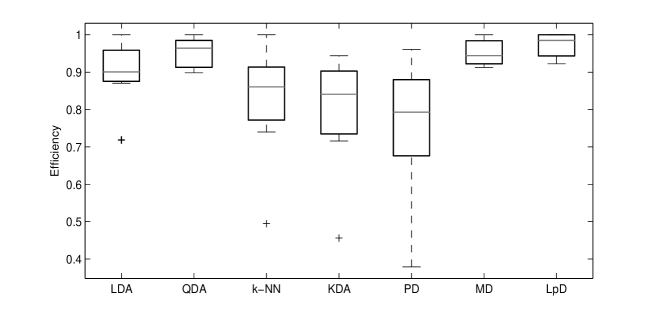
Figure 3: Overall performance of different classifiers on benchmark data sets.

For visual comparison of the overall performance among different classifiers, we computed their efficiencies for different data sets, and they are presented using boxplots in Figure 3. In a particular data set, the efficiency of a classifier $t$ is given by $e_{t}=\Delta_{0}/\Delta_{t}$, where $\Delta_{t}$ is the misclassification rate of the classifier $t$ and $\Delta_{0}=\min_{t}\Delta_{t}$. Clearly, $e_{t}=1$ for the best classifier, and $e_{t}<1$ for all other classifiers. Smaller values of $e_{t}$ indicates the lack of efficiency of the classifier $t$. Figure 3 clearly shows the superiority of the L_pD classifier over all other classifiers considered here.

Appendix: Proofs and Mathematical Details

Lemma 1: If the density $f(\mbox{\bf x},p)$ is of the form $\psi(\|{\bf A}(\mbox{\bf x}-{\bf b})\|_{p})$ for some $p>0$ and a continuous function $\psi:{\mathbb{R}}_{+}\rightarrow{\mathbb{R}}_{+}$, then it can be expressed as

$$f(\mbox{\bf x},p)=|{\bf A}|~{}\frac{p^{d-1}\Gamma(d/p)}{2^{d}\{\Gamma(1/p)\}^{d}}\frac{g_{p}(\delta_{p}(\mbox{\bf x}))\delta_{p}(\mbox{\bf x})^{d+1}}{[1-\delta_{p}(\mbox{\bf x})]^{d-1}}~{}\mbox{for}~{}0<\delta_{p}(\mbox{\bf x})<1,$$

where $\delta_{p}(\mbox{\bf x})=[1+\|{\bf A}(\mbox{\bf x}-{\bf b})\|_{p}]^{-1}$, and $g_{p}$ is the density function of $\delta_{p}(\mbox{\bf X})$ when $\mbox{\bf X}\sim f(\cdot,p)$.

Proof of Lemma 1: Define $\mbox{\bf Y}={\bf A}(\mbox{\bf X}-{\bf b})$. If $f_{0}$ denotes the density of Y, it is easy to see that $f_{0}(\mbox{\bf y})=|{\bf A}|^{-1}\psi(\|\mbox{\bf y}\|_{p})$. Now, following the proof of Lemma 1.4 in Fang, Kotz and Ng (1989), one can show that for any non-negative measurable function $\xi$, we have

$$\int_{\mathbb{R}^{d}}\xi(\|\mbox{\bf y}\|_{p})~{}d\mbox{\bf y}=\frac{2^{d}\{\Gamma(1/p)\}^{d}}{p^{d}\Gamma(d/p)}\int_{0}^{\infty}\xi(u^{1/p})u^{d/p-1}du.$$

So, for any non-negative measurable function $\phi$, defining $\xi=\phi.\psi$ we get

$$E[\phi(\|\mbox{\bf Y}\|_{p})] = |{\bf A}|^{-1}\int\phi(\|\mbox{\bf y}\|_{p})\psi(\|\mbox{\bf y}\|_{p})~{}d\mbox{\bf y}=|{\bf A}|^{-1}\frac{2^{d}\{\Gamma(1/p)\}^{d}}{p^{d}\Gamma(d/p)}\int_{0}^{\infty}\phi(u^{1/p})~{}\psi(u^{1/p})~{}u^{d/p-1}~{}du$$

$$= |{\bf A}|^{-1}\frac{2^{d}\{\Gamma(1/p)\}^{d}}{p^{d-1}\Gamma(d/p)}\int_{0}^{\infty}\phi(r)~{}\psi(r)~{}r^{d-1}~{}dr~{}(\mbox{letting}~{}r=u^{1/p}).$$

Therefore, the density of $r_{p}(\mbox{\bf X})=\|{\bf A}(\mbox{\bf X}-{\bf b})\|_{p}$ is the form ${\tau_{p}(r)=\displaystyle|{\bf A}|^{-1}\frac{2^{d}\{\Gamma(1/p)\}^{d}}{p^{d-1}\Gamma(d/p)}~{}\psi(r)~{}r^{d-1}}$, which implies $f(\mbox{\bf x},p)=\psi(r_{p}(\mbox{\bf x}))$ $=|{\bf A}|~{}\displaystyle\frac{p^{d-1}\Gamma(d/p)}{2^{d}\{\Gamma(1/p)\}^{d}}~{}\displaystyle\frac{\tau_{p}(r_{p}(\mbox{\bf x}))}{r_{p}(\mbox{\bf x})^{d-1}}.$ Recall that $\delta_{p}(\mbox{\bf x})=[1+r_{p}(\mbox{\bf x})]^{-1}$, and using the change of variables formula, we have the final expression for the density $f(\mbox{\bf x},p)$ in terms of $\delta_{p}(\mbox{\bf x})$ and its density $g_{p}(\cdot)$. $\Box$

Corollary 1: Define ${\tilde{\delta}}_{p}(\mbox{\bf x})=[1+a_{0}r_{p}(\mbox{\bf x})]^{-1}$, where $a_{0}$ is a positive constant, and let $g_{p}^{(a)}(\cdot)$ denote the density of ${\tilde{\delta}}_{p}(\mbox{\bf X})$. If the density $f(\mbox{\bf x},p)$ is of the form $\psi(\|{\bf A}(\mbox{\bf x}-{\bf b})\|_{p})$ for some $p>0$ and a continuous function $\psi:{\mathbb{R}}_{+}\rightarrow{\mathbb{R}}_{+}$, it can be expressed as

$$f(\mbox{\bf x},p)=a_{0}^{d}~{}|{\bf A}|~{}\frac{p^{d-1}\Gamma(d/p)}{2^{d}\{\Gamma(1/p)\}^{d}}\frac{g_{p}^{(a)}({\tilde{\delta}}_{p}(\mbox{\bf x})){\tilde{\delta}}_{p}(\mbox{\bf x})^{d+1}}{[1-{\tilde{\delta}}_{p}(\mbox{\bf x})]^{d-1}}~{}\mbox{for}~{}0<{\tilde{\delta}}_{p}(\mbox{\bf x})<1,$$

Proof of Corollary 1: If we define ${\tilde{r}}_{p}(\mbox{\bf x})=a_{0}r_{p}(\mbox{\bf x})$ and if $\tau^{(a)}_{p}(\cdot)$ denotes the density of ${\tilde{r}}_{p}(\mbox{\bf X})$, it is easy to check that $\displaystyle\frac{\tau_{p}(r_{p}(\mbox{\bf x}))}{r_{p}(\mbox{\bf x})^{d-1}}=a_{0}^{d}\displaystyle\frac{\tau_{p}^{(a)}({\tilde{r}}_{p}(\mbox{\bf x}))}{{\tilde{r}}_{p}(\mbox{\bf x})^{d-1}}$. Now from the proof of Lemma 1, it follows that $f(\mbox{\bf x},p)=a_{0}^{d}~{}|{\bf A}|~{}\displaystyle\frac{p^{d-1}\Gamma(d/p)}{2^{d}\{\Gamma(1/p)\}^{d}}~{}\displaystyle\frac{\tau_{p}^{(a)}({\tilde{r}}_{p}(\mbox{\bf x}))}{{\tilde{r}}_{p}(\mbox{\bf x})^{d-1}}.$ Since ${\tilde{\delta}}_{p}(\mbox{\bf x})=[1+{\tilde{r}}_{p}(\mbox{\bf x})]^{-1}$, the result is obtained by using the change of variables formula. $\Box$

Lemma 2: Let $f$ be $l_{p_{0}}$-symmetric for some $p_{0}\geq 1$. Define ${\tilde{\delta}}_{p}(\mbox{\bf x})$ and $g_{p}^{(a)}$ as in Corollary 1.
(i) If $\hat{{\bf b}}$ and ${\hat{\bf A}}$ satisfy assumption $(C1)$, for any $p\geq 1$, $\sup_{\mbox{\bf x}\in\mathbb{R}^{d}}|{\hat{\delta}}_{p}(\mbox{\bf x})-{\tilde{\delta}}_{p}(\mbox{\bf x})|=O_{P}(n^{-1/2})$.
(ii) Further, if the density $g_{p}$ and the bandwidth $h$ associated with the kernel density estimator ${\hat{g}}_{p,h}(\cdot)$ satisfies assumption $(C2)$, then $\sup_{\mbox{\bf x}\in\mathbb{R}^{d}}|{\hat{g}}_{p,h}(\hat{\delta}_{p}(\mbox{\bf x}))-g_{p}^{(a)}({\tilde{\delta}}_{p}(\mbox{\bf x}))|\stackrel{{\scriptstyle P}}{{\rightarrow}}0~{}\mbox{as}~{}n\rightarrow\infty$.

Proof of Lemma 2: (i) For any matrix A, let $\|\mbox{\bf A}\|_{F}=[trace(\mbox{\bf A}^{T}\mbox{\bf A})]^{1/2}$ denote its Frobenius norm and $\|\mbox{\bf A}\|_{p}=\sup_{\mbox{\bf x}}\{\|A\mbox{\bf x}\|_{p}/\|\mbox{\bf x}\|_{p}\}$ denote its $p$-th norm. For any $p\geq 1$, $\|\mbox{\bf A}\|_{p}$ is an induced norm that satisfies $\|\mbox{\bf A}\mbox{\bf x}\|_{p}\leq\|\mbox{\bf A}\|_{p}\|\mbox{\bf x}\|_{p}$ for all $\mbox{\bf x}\in{\mathbb{R}}^{d}$. In finite dimension, since all norms are equivalent, we have $\|\mbox{\bf A}\mbox{\bf x}\|_{p}\leq C_{p}\|\mbox{\bf A}\|_{F}\|\mbox{\bf x}\|_{p}$ for some positive constant $C_{p}$. This also implies that $\|\mbox{\bf x}\|_{p}\leq C_{p}\|\mbox{\bf A}^{-1}\|_{F}\|\mbox{\bf A}\mbox{\bf x}\|_{p}$, or $\|\mbox{\bf A}\mbox{\bf x}\|_{p}\geq\|\mbox{\bf x}\|_{p}/C_{p}\|\mbox{\bf A}^{-1}\|_{F}$.

Let us divide ${\mathbb{R}}^{d}$ into two disjoint regions: ${\cal R}_{1}=\{\mbox{\bf x}:\|\mbox{\bf x}\|\leq M\}$ and ${\cal R}_{2}=\{\mbox{\bf x}:\|\mbox{\bf x}\|>M\}$, where $M$ is a large positive constant. Note that $|\hat{\delta}_{p}(\mbox{\bf x})-\tilde{\delta}_{p}(\mbox{\bf x})|=\displaystyle\frac{|\hat{r}_{p}(\mbox{\bf x})-a_{0}{r}_{p}(\mbox{\bf x})|}{[1+\hat{r}_{p}(\mbox{\bf x})][1+a_{0}{r}_{p}(\mbox{\bf x})]}\leq|\hat{r}_{p}(\mbox{\bf x})-a_{0}{r}_{p}(\mbox{\bf x})|$. Using the triangle inequality, we obtain

$$\sqrt{n}\sup_{\mbox{\bf x}\in{\cal R}_{1}}|\hat{\delta}_{p}(\mbox{\bf x})-\tilde{\delta}_{p}(\mbox{\bf x})|\leq\sqrt{n}\sup_{\mbox{\bf x}\in{\cal R}_{1}}|\hat{r}_{p}(\mbox{\bf x})-a_{0}{r}_{p}(\mbox{\bf x})|\leq\|\hat{\mbox{\bf A}}\|_{F}\sqrt{n}\|\hat{\mbox{\bf b}}-\mbox{\bf b}\|_{p}+\sqrt{n}\|\hat{\mbox{\bf A}}-{a_{0}\mbox{\bf A}}\|_{F}\sup_{\mbox{\bf x}\in{\cal R}_{1}}\|\mbox{\bf x}-\mbox{\bf b}\|_{p}.\vspace{-0.1in}$$

Since $\sup_{\mbox{\bf x}\in{\cal R}_{1}}\|\mbox{\bf x}-\mbox{\bf b}\|_{p}\leq M+\|\mbox{\bf b}\|$, under the condition ($C1$), $\sup_{\mbox{\bf x}\in{\cal R}_{1}}\sqrt{n}|\hat{\delta}_{p}(\mbox{\bf x})-\tilde{\delta}_{p}(\mbox{\bf x})|=O_{p}(1)$. Also note that $|\hat{\delta}_{p}(\mbox{\bf x})-\tilde{\delta}_{p}(\mbox{\bf x})|\leq\displaystyle\frac{|\hat{r}_{p}(\mbox{\bf x})-a_{0}{r}_{p}(\mbox{\bf x})|}{[\hat{r}_{p}(\mbox{\bf x})][a_{0}{r}_{p}(\mbox{\bf x})]}$ and this implies that

$$\sqrt{n}|\hat{\delta}_{p}(\mbox{\bf x})-\tilde{\delta}_{p}(\mbox{\bf x})|\leq\displaystyle\frac{\|\hat{\mbox{\bf A}}\|_{F}\sqrt{n}\|\hat{\mbox{\bf b}}-\mbox{\bf b}\|_{p}}{(\|\hat{\mbox{\bf A}}\mbox{\bf x}\|_{p}-\|\hat{\mbox{\bf A}}\hat{\mbox{\bf b}}\|_{p})(\|{a_{0}\mbox{\bf A}}\mbox{\bf x}\|_{p}-\|{a_{0}\mbox{\bf A}}{\mbox{\bf b}\|}_{p})}+\frac{\sqrt{n}\|\hat{\mbox{\bf A}}-{(a_{0}\mbox{\bf A})}\|_{F}}{(\|\hat{\mbox{\bf A}}\mbox{\bf x}\|_{p}-\|\hat{\mbox{\bf A}}\hat{\mbox{\bf b}}\|_{p})a_{0}\|{\mbox{\bf A}}\|_{F}}.$$

Therefore, $\sqrt{n}\sup_{\mbox{\bf x}\in{\cal R}_{2}}|\hat{\delta}_{p}(\mbox{\bf x})-\tilde{\delta}_{p}(\mbox{\bf x})|$

$$\leq\displaystyle\frac{\|\hat{\mbox{\bf A}}\|_{F}\sqrt{n}\|\hat{\mbox{\bf b}}-\mbox{\bf b}\|_{p}}{[(M/\|\hat{\mbox{\bf A}}^{-1}\|_{F})-\|\hat{\mbox{\bf A}}\hat{\mbox{\bf b}}\|_{p}][(M/\|{C_{p}a_{0}\mbox{\bf A}}^{-1}\|_{F})-\|{a_{0}\mbox{\bf A}}{\mbox{\bf b}\|}_{p}]}+\frac{\sqrt{n}\|\hat{\mbox{\bf A}}-{(a_{0}\mbox{\bf A})}\|_{F}}{[M/\|\hat{\mbox{\bf A}}^{-1}\|_{F})-\|\hat{\mbox{\bf A}}\hat{\mbox{\bf b}}\|_{p}]a_{0}\|{\mbox{\bf A}}\|_{F}}.$$

In each of the two terms on the right side, the numerator is $O_{p}(1)$, while the denominator coverges to a positive constant. So, we have $\sqrt{n}\sup_{\mbox{\bf x}\in{\cal R}_{2}}|\hat{\delta}_{p}(\mbox{\bf x})-\tilde{\delta}_{p}(\mbox{\bf x})|=O_{p}(1)$. Now, combining the results on ${\cal R}_{1}$ and ${\cal R}_{2}$, the first part of the lemma is proved.

(ii) Note that $|{\hat{g}}_{p,h}(\hat{\delta}_{p}(\mbox{\bf x}))-g_{p}^{(a)}(\tilde{\delta}_{p}(\mbox{\bf x}))|\leq|\hat{g}_{p,h}(\hat{\delta}_{p}(\mbox{\bf x}))-\hat{g}_{p,h}(\tilde{\delta}_{p}(\mbox{\bf x}))|+|\hat{g}_{p,h}(\tilde{\delta}_{p}(\mbox{\bf x}))-g_{p}^{(a)}(\tilde{\delta}_{p}(\mbox{\bf x}))|.$ An application of the triangle inequality implies that

$$|\hat{g}_{p,h}(\hat{\delta}_{p}(\mbox{\bf x}))-\hat{g}_{p,h}(\tilde{\delta}_{p}(\mbox{\bf x}))|\leq\frac{1}{nh}\sum_{i=1}^{n}\left|K\left[\frac{\hat{\delta}_{p}(\mbox{\bf x})-\hat{\delta}_{p}(\mbox{\bf x}_{i})}{h}\right]\right.-\left.K\left[\frac{\tilde{\delta}_{p}(\mbox{\bf x})-\hat{\delta}_{p}(\mbox{\bf x}_{i})}{h}\right]\right|,$$

where $K$ is the kernel function associated with the density estimate. Using the mean value theorem and assuming $C_{K}=\sup_{x}|K^{\prime}(x)|<\infty$ (here we use the Gaussian kernel, which has bounded first derivative), we have $\sup_{\mbox{\bf x}\in\mathbb{R}^{d}}|\hat{g}_{p,h}(\hat{\delta}_{p}(\mbox{\bf x}))-\hat{g}_{p,h}(\tilde{\delta}_{p}(\mbox{\bf x}))|\leq C_{K}{\sup_{\mbox{\bf x}\in\mathbb{R}^{d}}|\hat{\delta}_{p}(\mbox{\bf x})-\tilde{\delta}_{p}(\mbox{\bf x})|}/{h^{2}}$. So, if $h$ satisfies the condition ($C2$), $~{}\sup_{\mbox{\bf x}\in\mathbb{R}^{d}}|\hat{g}_{p,h}(\hat{\delta}_{p}(\mbox{\bf x}))-\hat{g}_{p,h}(\tilde{\delta}_{p}(\mbox{\bf x}))|\stackrel{{\scriptstyle P}}{{\rightarrow}}0$ as $n\rightarrow\infty$.

To prove the convergence of $\sup_{\mbox{\bf x}\in\mathbb{R}^{d}}|\hat{g}_{p,h}(\tilde{\delta}_{p}(\mbox{\bf x}))-g_{p}^{(a)}(\tilde{\delta}_{p}(\mbox{\bf x}))|$, first note that

$$\sup_{\mbox{\bf x}\in\mathbb{R}^{d}}|\hat{g}_{p,h}(\tilde{\delta}_{p}(\mbox{\bf x}))-g_{p}^{(a)}(\tilde{\delta}_{p}(\mbox{\bf x}))|\leq\sup_{\mbox{\bf x}\in\mathbb{R}^{d}}|\hat{g}_{p,h}(\tilde{\delta}_{p}(\mbox{\bf x}))-g_{p,h}^{*}(\tilde{\delta}_{p}(\mbox{\bf x}))|+\sup_{\mbox{\bf x}\in\mathbb{R}^{d}}|g_{p,h}^{*}(\tilde{\delta}_{p}(\mbox{\bf x}))-g_{p}^{(a)}(\tilde{\delta}_{p}(\mbox{\bf x}))|,\vspace{-0.1in}$$

where $g_{p,h}^{*}(\tilde{\delta}_{p}(\mbox{\bf x}))={(nh)}^{-1}\sum_{i=1}^{n}K[\{\tilde{\delta}_{p}(\mbox{\bf x})-\tilde{\delta}_{p}(\mbox{\bf x}_{i})\}/{h}]$. So, using triangle inequality, one gets

$$\sup_{\mbox{\bf x}\in\mathbb{R}^{d}}|\hat{g}_{p,h}(\tilde{\delta}_{p}(\mbox{\bf x}))-g_{p}^{(a)}(\tilde{\delta}_{p}(\mbox{\bf x}))\leq\sup_{\mbox{\bf x}\in\mathbb{R}^{d}}|g_{p,h}^{*}(\tilde{\delta}_{p}(\mbox{\bf x}))-g_{p}^{(a)}(\tilde{\delta}_{p}(\mbox{\bf x}))|+C_{K}{\sup_{\mbox{\bf x}\in\mathbb{R}^{d}}|\hat{\delta}_{p}(\mbox{\bf x})-\tilde{\delta}_{p}(\mbox{\bf x})|}/{h^{2}}.\vspace{-0.1in}$$

We have already proved the convergence of the second term on the right side to $0$. Since $g_{p}$ is uniformly continuous and $nh/\log(n)\rightarrow\infty$ as $n\rightarrow\infty$ (see assumption (C2)), the convergence of the first term and hence the result now follow from the uniform convergence property of the kernel density estimate $g_{p,h}^{*}$ (see, e.g., Silverman, 1998).

Proof of Theorem 1: Define $A_{n}=\{\mbox{\bf x}:\tilde{\delta}_{p}(\mbox{\bf x})\in[\zeta_{1n},\zeta_{2n}]\}\subset\mathbb{R}^{d}$. Using the mean value theorem on the logarithmic function, one gets

$$\sup_{\mbox{\bf x}\in A_{n}}|\ln\hat{g}_{p,h}(\hat{\delta}_{p}(\mbox{\bf x}))-\ln g_{p}^{(a)}(\tilde{\delta}_{p}(\mbox{\bf x}))|\leq\sup_{\mbox{\bf x}\in\mathbb{R}^{d}}|\hat{g}_{p,h}(\hat{\delta}_{p}(\mbox{\bf x}))-g_{p}^{(a)}(\tilde{\delta}_{p}(\mbox{\bf x}))|\sup_{\mbox{\bf x}\in A_{n}}\left\{\frac{1}{\xi_{n}(\mbox{\bf x})}\right\},$$

where $\xi_{n}(\mbox{\bf x})=\lambda_{n}\hat{g}_{p,h}(\hat{\delta}_{p}(\mbox{\bf x}))+(1-\lambda_{n})g_{p}^{(a)}(\tilde{\delta}_{p}(\mbox{\bf x}))$ for some $\lambda_{n}\in(0,1)$. Hence, $\xi_{n}(\mbox{\bf x})$ converges to $g_{p}^{(a)}(\tilde{\delta}_{p}(\mbox{\bf x}))$ as $n\rightarrow\infty$ (follows from Lemma 2). From the proof of Lemma 2 and using a result on the rate of uniform consistency of the kernel density estimate (see Theorem B in Silverman, 1978, p. 181). Under (C2), we have $\sup_{\mbox{\bf x}\in\mathbb{R}^{d}}|\hat{g}_{p,h}(\hat{\delta}_{p}(\mbox{\bf x}))-g_{p}^{(a)}(\tilde{\delta}_{p}(\mbox{\bf x}))|=O_{P}(n^{-1/2}h^{-2})$. Therefore, using $(C3)$, we get $\sup_{\mbox{\bf x}\in A_{n}}|\ln\hat{g}_{p,h}(\hat{\delta}_{p}(\mbox{\bf x}))-\ln g_{p}^{(a)}(\tilde{\delta}_{p}(\mbox{\bf x}))|\stackrel{{\scriptstyle P}}{{\rightarrow}}0~{}\mbox{as}~{}n\rightarrow\infty$.

Following similar arguments as above, one can show that

$$\sup_{\mbox{\bf x}\in A_{n}}|\ln\hat{\delta}_{p}(\mbox{\bf x})-\ln(\tilde{\delta}_{p}(\mbox{\bf x}))|\leq\sup_{\mbox{\bf x}\in\mathbb{R}^{d}}|\hat{\delta}_{p}(\mbox{\bf x})-(\tilde{\delta}_{p}(\mbox{\bf x}))|\sup_{\mbox{\bf x}\in A_{n}}\left\{\frac{1}{\gamma_{n}(\mbox{\bf x})}\right\},$$

where $\gamma_{n}(\mbox{\bf x})$ = $\lambda_{n}\hat{\delta}_{p}(\mbox{\bf x})+(1-\lambda_{n})\tilde{\delta}_{p}(\mbox{\bf x})$ for some $\lambda_{n}\in(0,1)$, and it converges to $\tilde{\delta}_{p}(\mbox{\bf x})$. Since $\sup_{\mbox{\bf x}\in\mathbb{R}^{d}}|\hat{\delta}_{p}(\mbox{\bf x})-(\tilde{\delta}_{p}(\mbox{\bf x}))|=O_{P}(n^{-1/2})$ and $n^{1/2}\zeta_{1n}\rightarrow\infty$ as $n\rightarrow\infty$, we have $\sup_{\mbox{\bf x}\in A_{n}}|\log\hat{\delta}_{p}(\mbox{\bf x})-\log(\tilde{\delta}_{p}(\mbox{\bf x}))|$ $\stackrel{{\scriptstyle P}}{{\rightarrow}}0~{}\mbox{as}~{}n\rightarrow\infty$. Similarly, using the fact that $n^{1/2}(1-\zeta_{2n})\rightarrow\infty$ as $n\rightarrow\infty$, under the given conditions, one can show that $\sup_{\mbox{\bf x}\in A_{n}}|\log(1-\hat{\delta}_{p}(\mbox{\bf x}))-\log(1-{\tilde{\delta}}_{p}(\mbox{\bf x})))|\stackrel{{\scriptstyle P}}{{\rightarrow}}0~{}\mbox{as}~{}n\rightarrow\infty$. Combining these results and using corollary 1, we get $\sup_{\mbox{\bf x}\in A_{n}}|\ln\hat{f}_{n}(\mbox{\bf x},p)-\ln(a_{0}^{-d}f(\mbox{\bf x},p))|\stackrel{{\scriptstyle P}}{{\rightarrow}}0$ as $n\rightarrow\infty.$

Define the set $I_{n}=\{i:\mbox{\bf X}_{i}\in A_{n}\}$ and note that $\Bigl{|}\frac{1}{n}\sum_{i~{}\in I_{n}}\ln\hat{f}_{n}(\mbox{\bf x}_{i},p)-E_{p_{0}}\{\ln(a_{0}^{-d}f(\mbox{\bf X},p))\}\Bigr{|}\leq\sup_{\mbox{\bf x}\in A_{n}}|\ln\hat{f}_{n}(\mbox{\bf x},p)$ - $\ln(a_{0}^{-d}f(\mbox{\bf x},p))|$ $+\left|\frac{1}{n}\sum_{i~{}\in I_{n}}\ln(a_{0}^{-d}f(\mbox{\bf x}_{i},p))-E_{p_{0}}\{\ln(a_{0}^{-d}f(\mbox{\bf X},p))\}\right|,$ where $E_{p_{0}}$ denotes the expectation with respect to $f(\mbox{\bf x},p_{0})$. We have already proved the probability convergence of the first part on the right side to $0$. From the strong law of large numbers, we have $\left|\frac{1}{n}\sum_{i~{}\in I_{n}}\ln(a_{0}^{-d}f(\mbox{\bf x}_{i},p))-E_{p_{0}}\{\ln(a_{0}^{-d}f(\mbox{\bf X},p))I(\mbox{\bf X}\in A_{n})\}\right|\stackrel{{\scriptstyle a.s.}}{{\rightarrow}}0$ as $n\rightarrow\infty$.

Using monotone convergence theorem on the positive and negative parts of the integrand separately, we have $E_{p_{0}}\{\ln(a_{0}^{-d}f(\mbox{\bf X},p))I(\mbox{\bf X}\in A_{n})\}\rightarrow E_{p_{0}}\{\ln(a_{0}^{-d}f(\mbox{\bf X},p))\}~{}\mbox{as}~{}n\rightarrow\infty$. So, for all $p\geq 1$, we get $\frac{1}{n}\sum_{i~{}\in~{}I_{n}}\ln\hat{f}_{n}(\mbox{\bf x}_{i},p)\stackrel{{\scriptstyle P}}{{\rightarrow}}E_{p_{0}}\{\ln(a_{0}^{-d}f(\mbox{\bf X},p))\}=\ln(a_{0}^{-d})+E_{p_{0}}\{\ln f(\mbox{\bf X},p)\}$. One can notice that $E_{p_{0}}\{\ln f(\mbox{\bf X},p)\}=E_{p_{0}}\{\ln f(\mbox{\bf X},p_{0})\}-KL(p_{0},p)$, where $KL(p_{0},p)$ denotes the Kullback-Leibler divergence between $f(\mbox{\bf X},p_{0})$ and $f(\mbox{\bf X},p)$. So, maximization of $E_{p_{0}}\{\ln f(\mbox{\bf X},p)\}$ is equivalent to minimization of $KL(p_{0},p)$ over ${\cal P}$. Using Jensen’s inequality on the logarithmic function, we also have $E_{p_{0}}\{\ln f(\mbox{\bf X},p)\}<E_{p_{0}}\{\ln f(\mbox{\bf X},p_{0})\}$, or $KL(p_{0},p)>KL(p_{0},p_{0})$ for all $p\neq p_{0}$. Since ${\cal P}$ is a finite set, the proof now follows from the uniqueness of the minimizer of $KL(p_{0},p)$. $\Box$

Proof of Theorem 2: The misclassification rate of the classifier ${\sf d}_{1}$ is given by

$${\Delta({\sf d}_{1})=\frac{1}{J}\sum_{j=1}^{J}\int\theta_{j}(\mbox{\bf x},{\hat{p}_{n}})f_{j}(\mbox{\bf x},p_{0})~{}d\mbox{\bf x},}$$

where $\theta_{j}(\mbox{\bf x},{\hat{p}_{n}})=P\{\hat{\delta}_{{\hat{p}_{n}},j}(\mbox{\bf x})<\hat{\delta}_{{\hat{p}_{n}},i}(\mbox{\bf x})~{}\mbox{for some}~{}~{}i\neq j\}$. From the arguments given in the proof of Theorem 1, it follows that $\hat{p}_{n}\stackrel{{\scriptstyle P}}{{\rightarrow}}p_{0}$. Using the continuous mapping theorem, one gets $\hat{\delta}_{{\hat{p}_{n}},j}(\mbox{\bf x})\stackrel{{\scriptstyle P}}{{\rightarrow}}\tilde{\delta}_{p_{0},j}(\mbox{\bf x})$ for all $1\leq j\leq J$. So, if $\tilde{\delta}_{p_{0},j}(\mbox{\bf x})<\tilde{\delta}_{p_{0},i}(\mbox{\bf x})$ for all $i\neq j$ (or equivalently, $f_{j}(\mbox{\bf x},p_{0})>f_{i}(\mbox{\bf x},p_{0})$ for all $i\neq j$), $\theta_{j}(\mbox{\bf x},{\hat{p}}_{n})$ converges to $0$, otherwise it converges to $1$. Therefore, using the Dominated Convergence Theorem, we have the convergence of $\Delta({\sf d}_{1})$ to the Bayes risk. $\Box$

Lemma 3: If $p_{0}\in{\cal P}$, under $(C1)$ - $(C3)$, for any fixed $\mbox{\bf x}\in\mathbb{R}^{d}$, $\hat{f}_{h}(\mbox{\bf x},p_{0})\stackrel{{\scriptstyle P}}{{\rightarrow}}a_{0}^{-d}f(\mbox{\bf x},p_{0})$ as $n\rightarrow\infty$.

Proof of Lemma 3: Recall that $\displaystyle\hat{f}_{h}(\mbox{\bf x},p_{0})=C_{\hat{p}_{0},d}\frac{\hat{g}_{p_{0},h}(\hat{\delta}_{p_{0}}(\mbox{\bf x}))(\hat{\delta}_{p_{0}}(\mbox{\bf x}))^{d+1}}{(1-\hat{\delta}_{p_{0}}(\mbox{\bf x}))^{d-1}},$ where $C_{p,d}=\displaystyle\frac{p^{d-1}\Gamma(d/p)}{2^{d}\{\Gamma(1/p)\}^{d}}$. From the continuous mapping theorem and Theorem 1, we get $(\hat{\delta}_{\hat{p}_{n}}(\mbox{\bf x}))^{d+1}\stackrel{{\scriptstyle P}}{{\rightarrow}}(\tilde{\delta}_{p_{0}}(\mbox{\bf x}))^{d+1}$, $(1-\hat{\delta}_{\hat{p}_{n}}(\mbox{\bf x}))^{d-1}\stackrel{{\scriptstyle P}}{{\rightarrow}}(1-\tilde{\delta}_{p_{0}}(\mbox{\bf x}))^{d-1}~{}\mbox{for}~{}d>1$ and $\hat{g}_{\hat{p}_{0},h}({\delta}_{p_{0}}(\mbox{\bf x}))\stackrel{{\scriptstyle p}}{{\rightarrow}}g_{p_{0}}^{(a)}({\delta}_{p_{0}}(\mbox{\bf x}))$. The result now follows from Slutsky’s lemma and Corollary 1. $\Box$

Proof of Theorem 3 : For simplicity, we consider the case when $J=2$. For $J>2$, we use pairwise classification, and hence the result can be obtained by repeating the same argument for each of the $J(J-1)/2$ pairs of classes (see Tewari and Bartlett, 2007). Using Lemma 3, we get $(\hat{f}_{h_{1}}(\mbox{\bf x},p_{1}^{\circ}),\hat{f}_{h_{2}}(\mbox{\bf x},p_{2}^{\circ}))\stackrel{{\scriptstyle P}}{{\rightarrow}}(a_{1}^{-d}f(\mbox{\bf x},p_{1}^{\circ}),a_{2}^{-d}f(\mbox{\bf x},p_{2}^{\circ})),~{}\mbox{where}~{}a_{1},a_{2}>0$. Consider the classifier ${\sf d}_{2}^{p_{1}^{\circ},p_{2}^{\circ}}$ which is of the form:

$${\sf d}_{2}^{p_{1}^{\circ},p_{2}^{\circ}}(\mbox{\bf x})=\left\{\begin{array}[]{ll}1&~{}\mbox{if}~{}~{}\hat{f}_{h_{1}}(\mbox{\bf x},p_{1}^{\circ})/\hat{f}_{h_{2}}(\mbox{\bf x},p_{2}^{\circ})>k,\\ 2&~{}\mbox{otherwise}.\end{array}\right.$$

Here, $k$ is chosen by minimizing the leave-one-out cross-validation estimate of the misclassification probability. Note that for any fixed $k$, this cross-validation estimate is given by

$$\Delta^{CV}_{n,p_{1}^{\circ},p_{2}^{\circ}}(k)=\sum_{i=1,j\neq i}^{2}\frac{\pi_{i}}{n_{i}}\sum_{l=1}^{n_{i}}I\left[\Bigl{\{}{\hat{f}_{h_{i}}^{-il}(\mbox{\bf x}_{il},p_{i}^{\circ})}/{\hat{f}_{h_{j}}^{-il}(\mbox{\bf x}_{jl},p_{j}^{\circ})}\Bigr{\}}\leq k_{i}\right],$$

where $n=(n_{1},n_{2})$, $k_{1}=k$, $k_{2}=1/k$, and ${\hat{f}}_{h_{j}}^{-il}$ denotes the leave-one-out density estimate with $\mbox{\bf x}_{il}$ being left out as a training data point. Let $k_{n}$ denote the minimizer of $\Delta_{n,p_{1}^{\circ},p_{2}^{\circ}}^{CV}(k)$.

Define

$$\Delta_{p_{1}^{\circ},p_{2}^{\circ}}(k)=\sum_{i=1,j\neq i}^{2}\pi_{i}P\left[\Bigl{\{}{a_{i}^{-d}f(\mbox{\bf X},p_{i}^{\circ})}/{a_{j}^{-d}f(\mbox{\bf X},p_{j}^{\circ})}\Bigr{\}}\leq k_{i}~{}\biggr{|}~{}\mbox{\bf X}\in i\mbox{-th class}\right],$$

and $k_{0}=\arg\min_{k}\Delta_{p_{1}^{\circ},p_{2}^{\circ}}(k)$. Under the stated assumptions, $k_{0}=a_{1}^{-d}\pi_{2}/a_{2}^{-d}\pi_{1}$ is a unique solution, and $0<k_{0}<\infty$. Note that $\Delta_{p_{1}^{\circ},p_{2}^{\circ}}(k_{0})$ denotes the misclassification probability of the Bayes classifier ${\sf d}_{B}$. Consistency of the density estimates and using the same arguments as in Lemma 3 of Dutta and Ghosh (2012), one can show that $\sup_{k}|\Delta_{n,p_{1}^{\circ},p_{2}^{\circ}}^{CV}(k)-\Delta_{p_{1}^{\circ},p_{2}^{\circ}}(k)|\stackrel{{\scriptstyle P}}{{\rightarrow}}0$. This now implies that $k_{n}\stackrel{{\scriptstyle P}}{{\rightarrow}}k_{0}$ as $\min\{n_{1},n_{2}\}\rightarrow\infty$. So, using the continuous mapping theorem and continuity of the underlying densities, we have ${\sf d}_{2}^{p_{1}^{\circ},p_{2}^{\circ}}(\mbox{\bf x})\stackrel{{\scriptstyle P}}{{\rightarrow}}{\sf d}_{B}(\mbox{\bf x})$ for any fixed $\mbox{\bf x}\in\mathbb{R}^{d}$ not lying on the Bayes class boundary. Using the Dominated Convergence Theorem, we can show that the misclassification probability of the classifier ${\sf d}_{2}^{p_{1}^{\circ},p_{2}^{\circ}}$ has the following convergence:

$$\Delta_{2}^{p_{1}^{\circ},p_{2}^{\circ}}=\sum_{i=1}^{2}\pi_{i}~{}P[{\sf d}_{2}^{p_{1}^{\circ},p_{2}^{\circ}}(\mbox{\bf X})\neq i\mid\mbox{\bf X}\sim f(\cdot,p_{i}^{\circ})]\rightarrow\sum_{i=1}^{2}\pi_{i}~{}P[{\sf d}_{B}(\mbox{\bf X})\neq i\mid\mbox{\bf X}\sim f(\cdot,p_{i}^{\circ})]=\Delta_{B},$$

the Bayes risk as $\min\{n_{1},n_{2}\}\rightarrow\infty$.

From Theorem 1, we have ${\hat{p}_{1n_{1}}}\stackrel{{\scriptstyle P}}{{\rightarrow}}p_{1}^{\circ}$ and ${\hat{p}_{2n_{2}}}\stackrel{{\scriptstyle P}}{{\rightarrow}}p_{2}^{\circ}$ as $n\to\infty$. Since ${\cal P}$ is finite, this implies $P({\hat{p}_{1n_{1}}}=p_{1}^{\circ},{\hat{p}_{2n_{2}}}=p_{2}^{\circ})\rightarrow 1$ as $n\rightarrow\infty$. The misclassification probability of the classifier ${\sf d}_{2}$ can be expressed as follows:

$$\sum_{p_{1}\in{\cal P}}\sum_{p_{2}\in{\cal P}}\Delta_{2}^{p_{1},p_{2}}~{}P({\hat{p}_{1n_{1}}}=p_{1},{\hat{p}_{1n_{1}}}=p_{2}).$$

It is now straight forward to prove that the expression above converges to $\Delta_{2}^{p_{1}^{\circ},p_{2}^{\circ}}(=\Delta_{B},\mbox{ the Bayes risk})$ as $\min\{n_{1},n_{2}\}\to\infty$. $\Box$

References

• [1] Arellano-Valle, R. B. and Richter, W.-D. (2012) On skewed continuous $l_{n,p}$-symmetric distributions. Chilean J. Statist., 3, 193-212.
• [2] Cator, E. A. and LopuhaΓ€, H. P. (2012) Central limit theorem and influence function for the MCD estimators at general multivariate distributions. Bernoulli, 18, 520-551.
• [3] Chakraboty, B. and Chaudhuri, P. (1996) On a transformation and re-transformation technique for constructing affine equivariant multivariate median. Proc. Amer. Math. Soc., 124, 2539-2547.
• [4] Chakraborty, B. (2001) On affine equivariant multivariate quantiles. Ann. Inst. Statist. Math., 53, 380-403.
• [5] Cui, X., Lin, L. and Yang, G. (2008) An extended projection data depth and its applications to discrimination. Comm. Statist. Theory Methods, 37, 2276-2290.
• [6] Duda, R. O., Hart, P. E. and Stork, D. G. (2012) Pattern Classification, Wiley, New York.
• [7] Dutta, S., Ghosh, A. K. and Chaudhuri, P. (2011) Some intriguing properties of Tukey’s half-space depth. Bernoulli, 17, 1420-1434.
• [8] Dutta, S. and Ghosh, A. K. (2012) On robust classification using projection depth. Ann. Inst. Statist. Math., 64, 657-676.
• [9] Fang, K. -T., Kotz, S. and Ng, K. -W. (1989) Symmetric Multivariate and Related Distributions. Chapman and Hall, London.
• [10] Fraiman, R., Liu, R. Y. and Meloche, J. (1997) Multivariate density estimation by probing depth. In $L_{1}$-Statistical Procedures and Related Topics. IMS Lecture Notes (Ed. Y. Dodge), Inst. Math. Statist., Hayward, California, 31, 415-430.
• [11] Ghosh, A. K. and Chaudhuri, P. (2005) On maximum depth and related classifiers. Scand. J. Statist., 32, 328-350.
• [12] Ghosh, A. K. and Hall, P. (2008) On error rate estimation in nonparametric classification. Statistica Sinica, 18, 1081-1100.
• [13] Gupta, A. K. and Song, D. (1997) Lp norm spherical distribution. J. Statist. Plan. Infer., 60, 241-260.
• [14] Hartikainen, A. and Oja, H. (2006) On nonparametric discrimination rules. In Data Depth: Robust Multivariate Analysis, Computational Geometry, and Applications (Eds. R. Liu, R. SerflΒ‚ing and D. Souvaine), Amer. Math. Soc., 72, 61-70.
• [15] Hastie, T., Tibshirani, R. and Friedman, J. (2009) Elements of Statistical Learning Theory. Wiley, New York.
• [16] Hubert, M. and van Driessen, K. (2004) Fast and robust discriminant analysis. Comput. Statist. Data Anal., 45, 301-320.
• [17] Hoberg, R. and Mosler, K. (2006) Data analysis and classification with the zonoid depth. In Data Depth: Robust Multivariate Analysis, Computational Geometry and Applications (Eds. R. Liu, R. SerflΒ‚ing and D. Souvaine), Amer. Math. Soc., 72, 49-59.
• [18] Johnson, R. A. and Wichern, D. W. (1992) Applied Multivariate Statistical Analysis. Prentice-Hall, New Jersey.
• [19] JΓΆrnsten, R. (2004) Clustering and classification based on the L1 data depth. J. Multivar. Anal., 90, 67-89.
• [20] Li, J., Cuesta-Albertos, J. A. and Liu, R. (2012) Nonparametric classification procedures based on DD-plot. J. Amer. Statist. Assoc., 107, 737-753.
• [21] Liu, R., Parelius, J. and Singh, K. (1999) Multivariate analysis of the data-depth : Descriptive statistics and inference. Ann. Statist., 27, 783-858.
• [22] Paindaveine, D. and Van Bever, G. (2015) Nonparametrically consistent depth-based classifiers. Bernoulli, 21, 62-82.
• [23] Sheather, S. J. and Jones, M. C. (1991) A reliable data based bandwidth selection method for kernel density estimation. J. Royal Statist. Soc. Ser. B, 53, 683-690.
• [24] Silverman, B. W. (1978) Weak and strong uniform consistency of the kernel estimate of a density and its derivatives. Ann. Statist., 6, 177-184.
• [25] Silverman, B. W. (1998) Density Estimation for Statistics and Data Analysis. Chapman and Hall, London.
• [26] Sinz, F. and Bethge, M. (2010) Lp-nested symmetric distributions. J. Mach. Learn. Res., 11, 3409-3451.
• [27] Tewari, A. and Bartlett, P. L. (2007) On the consistency of multiclass classification methods. J. Mach. Learn. Res., 8, 1007-1025.
• [28] Tukey, J. W. (1975) Mathematics and the picturing of data. Proc. 1975 Inter. Cong. Math., Vancouver, 523-531.
• [29] Yue, X. and Ma, C. (1995) Multivariate Lp-norm symmetric distributions. Statist. Probab. Letters, 24, 281-288.
• [30] Zuo, Y. and Serfling, R. (2000) General notions of statistical depth function. Ann. Statist., 28, 461-482.