Cluster Monte Carlo and dynamical scaling for long-range interactions

Abstract

Many spin systems affected by critical slowing down can be efficiently simulated using cluster algorithms. Where such systems have long-range interactions, suitable formulations can additionally bring down the computational effort for each update from O($N^{2}$) to O($N\ln N$) or even O($N$), thus promising an even more dramatic computational speed-up. Here, we review the available algorithms and propose a new and particularly efficient single-cluster variant. The efficiency and dynamical scaling of the available algorithms are investigated for the Ising model with power-law decaying interactions.

1 Introduction

The theory of phase transitions and critical phenomena is by now rather well understood, although there remain a significant number of questions that are still very actively debated and some of which are not finally settled, ranging from the theory of disordered systems kawashima:03a ; fytas:16 to quite fundamental problems such as certain aspects of finite-size scaling wittmann:14 ; flores:16 . The theoretical basis of this success is the concept of the renormalization group fisher:74a that allows one to understand scaling and universality in such systems. While this theory provides the essential scaffolding for describing continuous phase transitions, and many results have been derived from it via perturbative approaches such as the $\epsilon$ expansion, the field is now hardly conceivable without contributions from numerical techniques such as the molecular dynamics rapaport:04 and Monte Carlo methods binder:book2 . While the basic techniques such as, e.g., the Metropolis algorithm metropolis:53a for simulations of spin systems, are rather easily implemented, using them for studies of critical points is not straightforward as there the simulational and the physical dynamics are affected by critical slowing down due to the proliferation of spatial correlations as the critical point is approached. An effective antidote for this problem is available in the form of cluster algorithms as originally proposed for the short-range Ising model swendsen-wang:87a ; wolff:89a and later generalized to a range of different spin models and certain off-lattice systems luijten:06 . They manage to substantially reduce or, in some cases, practically eliminate critical slowing down through the identification and updating of large-scale, fractal structures whose extent diverges as the critical point is approached. A related class of algorithms even achieve critical speeding up, an increase of computational efficiency with system size, for certain quantities deng:07 ; elci:13 .

While the electromagnetic force as the basic agent in condensed-matter systems decays slowly, proportional to the inverse square of the distance, due to screening effects short-range intermolecular interactions such as those parameterized in the Lennard-Jones potential dominate in many cases. In some systems, however, such as in frustrated magnets lacroix:11 or in certain lattices of cold atoms britton:12 , long-range interactions are responsible for the presence or absence of ordering. The effect of such interactions on the nature of the transition was studied early on in the framework of the renormalization group fisher:72 . Apart from describing experimentally relevant systems with long-range interactions, these models were also soon recognized as pathways for introducing non-trivial critical behavior into systems whose physical dimension is too low to exhibit such ordering for short-range couplings dyson:69 ; dyson:71 . While both local and cluster-update Monte Carlo simulation algorithms are directly applicable to systems with long-range interactions, the fact that each particle or spin interacts with all others implies an $O(N^{2})$ scaling of the computational effort for the simulation of a system of $N$ particles. As a result, the system sizes accessible computationally through these methods are severely restricted, typically to a few thousand spins xu:93 . Due to this limitation, many studies considered cut-offs to the interactions and/or extrapolation methods to try to access ranges of system sizes where finite-size scaling approaches could be meaningfully employed nagle:70 ; glumac:89 . It was realized by Luijten and Blöte luijten:95 that these restrictions could be lifted using a different formulation of the cluster algorithm that allows one to update all spins once with an $O(N\log N)$ computational effort. More recently, Fukui and Todo fukui:09 proposed a related, slightly more general approach with a scaling only slightly worse than linear. Below, we discuss a single-cluster variant with strictly $O(N)$ scaling. These methods hence deliver a twofold and very dramatic speedup: a computational acceleration from $O(N^{2})$ to $O(N)$ operations per sweep and, in addition, a reduction of critical slowing down in the vicinity of the critical point.

The rest of the paper is organized as follows. In Sec. 2 we give a short summary of the Swendsen-Wang algorithm to set the stage for the improved methods. Sections 3 and 4 discuss the Luijten-Blöte and Fukui-Todo approaches, respectively, including the single-cluster variant introduced here. The computational and algorithmic performance is discussed in Sec. 5. Finally, Sec. 6 contains our conclusions.

2 Swendsen-Wang algorithm

Although the algorithms discussed below can be generalized to the case of Potts and even continuous-spin models, for the sake of simplicity we restrict our presentation to the case of the Ising model with Hamiltonian

$${\cal H}=-\sum_{i,j}J_{ij}s_{i}s_{j}-\sum_{i}H_{i}s_{i},\;\;\;s_{i}=\pm 1.$$ (1)

Here, the sum is over all lattice sites, $J_{ij}$ is the exchange coupling between spins $i$ and $j$ and $H_{i}$ denotes a local external magnetic field. Unless stated otherwise, we will focus on the case of zero external fields, $H_{i}=0$.

Let us first consider the case of homogeneous nearest-neighbor interactions, $J_{ij}=J$ if $i$, $j$ are nearest neighbors on the lattice and $J_{ij}=0$ otherwise. It is straightforward to verify the following identities for the partition function of the model wj:chem ,

$$\begin{split}Z&=\sum_{\{s_{i}\}}\exp\left(\beta J\sum_{\langle i,j\rangle}s_{i}s_{j}\right)\\ &=\sum_{\{s_{i}\}}\prod_{\langle i,j\rangle}e^{\beta J}\left[(1-p)+p\delta_{s_{i},s_{j}}\right]\\ &=\sum_{\{s_{i}\}}\sum_{n_{ij}}\prod_{\langle i,j\rangle}e^{\beta J}\left[(1-p)\delta_{n_{ij},0}+p\delta_{s_{i},s_{j}}\delta_{n_{ij},1}\right]\\ &=\sum_{\{s_{i}\}}\sum_{n_{ij}}\prod_{\langle i,j\rangle}W(s_{i},s_{j},n_{ij}).\end{split}$$ (2)

Here, $n_{ij}\in\{0,1\}$ are new, binary variables that represent the state of the bonds as ‘active’ or ‘deleted’, and $p=1-\exp(-2\beta J)$ is the bond activation probability. The form (2) corresponds to the Fortuin-Kasteleyn (FK) representation of the Ising model fortuin:72a . This transformation from a pure spin model to a probability measure jointly defined on spins and ‘graph’ variables (i.e., bonds), known as the Edwards-Sokal coupling edwards:88a , is at the heart of all cluster updates of this type. The representation (2) implies the following update procedure known as the Swendsen-Wang algorithm swendsen-wang:87a for the ferromagnetic, nearest-neighbor Ising model:

1. Activate bond variables, i.e., set $n_{ij}=1$, between neighboring spins with probability $P_{ij}=\delta_{s_{i},s_{j}}p$.

2. Identify clusters of spins connected by active bonds.

3. Flip independent clusters with probability $1/2$.

This generates a new spin configuration which is then subjected to a new iteration of the same procedure etc. As it is possible to have single-site clusters, the algorithm is ergodic. Together with detailed balance, which can be shown quite straightforwardly by inspecting the configuration weight $W(s_{i},s_{j},n_{ij})$ in the joint spin and bond space, this guarantees that the underlying Markov chain converges to the equilibrium stationary distribution binder:book2 . For the best possible choices of the algorithm used for cluster identification weigel:10b , one full update of the Swendsen-Wang algorithm requires $O(N+E)$ operations, where $N$ is the number of spins and $E$ is the number of edges in the graph. For a short-range lattice model, $E=zN/2$, where $z$ is the coordination number, resulting in $O(N)$ scaling.

Consider now a long-range model where, in general, all $J_{ij}$ are non-zero and different. The FK representation (2) is easily generalized to this case by noting that the weight function is now

$$W(s_{i},s_{j},n_{ij})=e^{\beta J_{ij}}\left[(1-p_{ij})\delta_{n_{ij},0}+p_{ij}\delta_{s_{i},s_{j}}\delta_{n_{ij},1}\right],$$

where the bond dependent activation probability is

$$p_{ij}=1-\exp(-2\beta J_{ij}).$$

Note that there is a subtlety in the notation here, with $P_{ij}=\delta_{s_{i},s_{j}}p_{ij}$ being the activation probability for the bond between $i$ and $j$, while $p_{ij}$ is the activation probability conditioned on $s_{i}=s_{j}$. The resulting cluster algorithm still satisfies ergodicity and detailed balance, so is correct. As $E=N^{2}-N$, however, one update is now much more expensive, and we expect $O(N^{2})$ run-time scaling asymptotically, much like that for single spin updates.

A variant of the Swendsen-Wang algorithm due to Wolff wolff:89a grows and flips only a single cluster, emanating from a single, randomly chosen seed site, thus reducing the effort for cluster identification (which can be done on the fly) and leads to larger clusters being flipped, such that it is typically more efficient. While run times are now proportional to the number of edges in a given cluster, the number of operations required to update each spin once on average remains $O(N^{2})$.

3 Luijten-Blöte algorithm

Thus, while the Swendsen-Wang or Wolff (single cluster) algorithms naturally extend to the case of long-range interactions, their direct application leads to $O(N^{2})$ scaling. Luijten and Blöte luijten:95 noticed that in the interesting regime of couplings and temperatures most probabilities $p_{ij}$ will be very small and so there are many rejected bond activation attempts. These can be avoided by directly sampling from the cumulative distribution of bond probabilities. To see this, consider for definiteness a system with power-law interactions,

$$J_{ij}=\frac{J}{r_{ij}^{d+\sigma}}.$$ (3)

The bond activation probabilities are then $p_{ij}=1-\exp(-2\beta J/r_{ij}^{d+\sigma})\equiv p_{r}$, and only depend on the distance $r=r_{ij}$ of lattice sites. In the following, we only make use of this translational invariance and not of the specific power-law form of Eq. (3). We first consider the special case of a chain, i.e., lattice dimension $d=1$. The algorithm is a single-cluster variant, where spins are added successively to the cluster starting from an initial, random seed site by probing the bonds emanating from the currently considered spin for activation. If the current spin is at site $i$, we consider spins at sites $j$ to be added in the order of increasing distance $|j-i|$ along the chain. The probability that the first bond connecting to $i$ to be activated in this way is the spin at site $k$ is

$$q(k)=(1-p_{1})(1-p_{2})\cdots(1-p_{k-1})p_{k}.$$

We can pick a site $k$ according to this probability by considering the cumulative distribution,

$$C(k)=\sum_{n=1}^{k}q(n)=1-\prod_{n=1}^{k}(1-p_{n}).$$ (4)

If a random number $r$ drawn uniformly in $[0,1[$ is found to be between $C(k-1)$ and $C(k)$, the next spin to be added to the cluster is at distance $k$. The next bond after that must be drawn between the current spin $i$ and another spin at distance $l>k$, and so the relevant probability is

$$q_{k}(l)=(1-p_{k+1})(1-p_{k+2})\cdots(1-p_{l-1})p_{l},$$

and we need to sample from the cumulative distribution

$$C_{k}(l)=\sum_{n=k+1}^{l}q_{k}(n)=1-\prod_{n=k+1}^{l}(1-p_{n}),$$ (5)

such that $C(k)=C_{0}(k)$. For the third and higher spins we proceed iteratively along the same lines.

Note that for free boundaries we also need to allow for the possibility of activating bonds to spins with $k<i$, i.e., to the left of the current spin. This can be taken into account by formally using an interaction strength $2J$ instead of $J$ and using an extra random number for each activated bond to decide whether it is to a spin to the left or to the right of the current one. For periodic boundaries, on the other hand, the distance definition to use (for the chain) is modified to $r_{ij}=\min(|i-j|,L-|i-j|)$.

This leaves us to decide how efficiently one can sample from the cumulative distributions (4) and (5), respectively. We note that $C(k)$ and $C_{k}(l)$ are related by a linear transformation,

$$C_{k}(l)=\frac{p_{k+1}}{q(k+1)}\left[C(l)-C(k)\right],$$

such that it is sufficient to store $N$ elements in such a look-up table for a translationally invariant system. In the most naive implementation, we would require a number of comparisons that is $O(N)$ to decide in which bin the random number $r$ falls. This can be of course be avoided using a binary search in a table of the probabilities $C_{k}(l)$, reducing the effort to a factor $\log N$. If one wants to truncate the interaction to reduce the storage and time effort for look-ups, this works less well in higher dimensions as the number of distinct lattice distances to store in the vicinity of the seed site grows quickly with $d$. Luijten and Blöte hence suggest luijten:95 ; luijten:97 to modify the interaction potential in a way that allows for an analytic inversion of the cumulative distribution function and to thus avoid the lookup tables altogether. This will not lead to correct results for the original model considered, but it can be an affordable simplification if one is only interested in universal quantities which are independent of such details. A direct generalization of the exact algorithm to higher dimensions is feasible, but a little bit tedious due to the necessary bookkeeping.

The approach of Luijten and Blöte thus entails a computational effort of $O(\log E)=O(\log N)$ for the look-up of each weight (even in the non-translationally invariant case), and since there are on average $O(N)$ active bonds in the regime where the potential (3) is integrable fukui:09 , the total effort is $O(N\log N)$.

4 Fukui-Todo algorithm

The cluster update could be simplified further if one could decide about the number of active bonds at the onset and place them according to the local bond weights. This is in fact possible if one allows the bond activation variables that are restricted to $n_{ij}\in\{0,1\}$ following the FK representation to take arbitrary, non-negative integer values $n_{i,j}=0$, $1$, $2$, $\ldots$ fukui:09 . This is compatible with the FK weight if one ensures that the probability of a non-zero $n_{ij}$ for parallel spins is identical to the standard bond activation probability $p_{ij}$, i.e.,

$$\mathbb{P}(n_{ij}>0|s_{i}=s_{j})=\sum_{n_{ij}=1}^{\infty}f(n_{ij})=p_{ij}=1-e^{-2\beta J_{ij}}.$$ (6)

Instead of the binary distribution $f(n_{ij})=(1-p_{ij})\delta_{n_{ij},0}+p_{ij}\delta_{n_{ij},1}$ of the standard FK model, we now choose a Poisson distribution,

$$f_{\lambda}(n)=\frac{e^{-\lambda}\lambda^{n}}{n!},$$ (7)

where the normalization condition (6) implies that $\lambda_{ij}=2\beta J_{ij}$. This can be formally incorporated into a generalized FK representation by noting that the FK weight can be factorized into the $p_{ij}$ dependent part that only contains $n_{ij}$, while the remainder depending on $s_{i}s_{j}$ is independent of $p_{ij}$,

$$W(s_{i},s_{j},n_{ij})=e^{\beta J_{ij}}V(n_{ij})\Delta(s_{i},s_{j},n_{ij}),$$

where

$$\begin{split}V(n_{ij})&=(1-p_{ij})\delta_{n_{ij},0}+p_{ij}\delta_{n_{ij},1},\\ \Delta(s_{i},s_{j},n_{ij})&=\delta_{n_{ij},0}+\delta_{s_{i},s_{j}}\delta_{n_{ij},1}.\end{split}$$ (8)

We can therefore write down the FK representation of the model with general integer bond variables,

$$\begin{split}V(n_{ij})&=\frac{e^{-2\beta J_{ij}}(2\beta J_{ij})^{n_{ij}}}{n_{ij}!},\\ \Delta(s_{i},s_{j},n_{ij})&=\delta_{n_{ij},0}+(1-\delta_{n_{ij},0})\delta_{s_{i},s_{j}}.\end{split}$$ (9)

The advantage of allowing the bond variables to take on arbitrary integer values $n_{ij}\geq 0$ according to a Poisson distribution is that any (finite or infinite) sum of Poisson random variables, even of different means, leads again to a Poisson distribution, i.e., it is a sum-stable distribution. Additionally, we have the following distribution identity,

$$\prod_{(i,j)}f_{\lambda_{ij}}(n_{ij})=f_{\lambda_{\mathrm{tot}}}(n_{\mathrm{tot}})\frac{n_{\mathrm{tot}}!}{\prod_{(i,j)}n_{ij}!}\prod_{(i,j)}\left(\frac{\lambda_{ij}}{\lambda_{\mathrm{tot}}}\right)^{n_{ij}},$$ (10)

where $(i,j)$ denotes the (undirected) bond connecting the sites $i$ and $j$ on the lattice. The left-hand side corresponds to drawing each $n_{ij}$ independently according to $f_{\lambda_{ij}}$. The right-hand side, on the other hand, represents a prescription where a total number $n_{\mathrm{tot}}$ is drawn according to $f_{\lambda_{\mathrm{tot}}}$ with $\lambda_{\mathrm{tot}}=\sum_{(i,j)}\lambda_{ij}=\sum_{(i,j)}2\beta J_{ij}=2\beta J_{\mathrm{tot}}$ first and these ‘events’ are then randomly distributed over the actual bonds with a probability $\lambda_{ij}/\lambda_{\mathrm{tot}}$. The equation expresses the fact that these two procedures lead to the same final distribution of $n_{ij}$. The distribution of events can be performed using tables with binary search as for the approach of Luijten and Blöte or, alternatively, using Walker’s method of alias, as will be discussed below in Sec. 4.1.

4.1 Multi-cluster method

The modified FK representation can be used to simulate the underlying Ising model as follows:

1. Draw a total number of events $n_{\mathrm{tot}}\geq 0$ according to a Poisson distribution with mean $\lambda_{\mathrm{tot}}=2\beta\sum_{(ij)}J_{ij}$.

2. Distribute each event to one of the bonds with probability $\lambda_{ij}/\lambda_{\mathrm{tot}}$.

3. Identify clusters of like spins connected by bonds with $n_{ij}>0$ and flip each cluster with probability $1/2$.

The normalization (6) ensures that the actual spin dynamics of this approach is the same as that of the Swendsen-Wang approach. It is different, however, from the Luijten-Blöte algorithm in the same sense as the Wolff algorithm is different from Swendsen-Wang dynamics since in the single-cluster algorithm on average larger clusters are flipped.

Let us discuss some implementation details and the computational complexity of each step of the approach. The most straightforward algorithms for generating Poisson random variates have running time proportional to $\lambda$ knuth:vol2 , but there exist methods whose run-time is independent of the mean gentle:03 . In any case, as $\lambda_{\mathrm{tot}}=2\beta J_{\mathrm{tot}}$ this is $O(E)$, in general, but reduces to $O(N)$ for the relevant case of energy-integrable couplings (i.e., $\sigma>0$ for the Ising FM in one dimension). In this case, the total number of events to distribute is $O(N)$. The distribution of events in the second step is performed using a look-up operation. Specifically, if we use the shorthand $p_{k}$, $k=1,\ldots,E$ for the probabilities $\lambda_{ij}/\lambda_{\mathrm{tot}}$, one draws a random number $r$ uniformly in $[0,1[$. If $r<p_{1}$ the event is allocated to edge 1. Alternatively, if $r<p_{1}+p_{2}$ the event is allocated to edge 2 etc. While this approach has $O(E)$ scaling, it can easily be sped up by a binary (bisection) search in the table $\sum_{i<j}p_{i}$ of cumulative probabilities, bringing the computational effort down to $O(\ln E)$.

As it turns out, however, also this simplification is not optimal and a faster method is provided by Walker’s method of alias that can be outlined as follows: one first sets up a table $U_{k}=Ep_{k}$ and tries to sample from the distribution $p_{k}$ by selecting one of the entries in the table with a uniform random number in $[1,E]$. This would only be correct, however, if each $U_{k}=1$. In reality, there are “over-full” bins $U_{k}>1$ and “under-full” bins $U_{k}<1$. One now starts a procedure of re-distributing the extraneous weight from over-full bins to under-full ones, keeping track of the origin of weights using an alias table $A_{k}$. Once these tables are set up, perfect samples can be drawn from $p_{k}$ using just two uniform random numbers, one to index into $U_{k}$ and a second one for the alias table $A_{k}$. Details can be found in Refs. knuth:vol2 ; fukui:09 . This approach provides look-ups and distribution of an event in constant time.

For the cluster identification it is not convenient to store the bond states as is sometimes done for short-range models as this would bring the computational (and storage) effort up to $O(N^{2})$ again. Instead, we make use of the tree-based union-and-find method, where the cluster structure is stored as a forest of trees (implemented as an array of pointers). Each time a previously deleted bond is activated, connectivity queries decide whether the connected nodes belong to different trees, in which case one of the trees is attached to the other at the current leaf. While for a naive implementation connectivity queries and bond insertion have $O(N)$ scaling, additional heuristics known as path compression and tree balancing bring the run-time scaling down to $O(\log N)$ if employing one of these heuristics or even almost $O(1)$ if both tricks are combined. Details of this approach can be found in Refs. knuth:vol2 ; newman:01a ; elci:13 .

As a result, the Fukui-Todo approach shows run-time scaling that is, for all practical purposes, indistinguishable from $O(N)$ for systems with energy convergent couplings. This includes the mean-field model, where couplings are normally chosen to be $J_{ij}=1/N$ to ensure a finite energy in the thermodynamic limit. The storage requirement is $O(E)$ for the look-up table in the bond distribution step, whereas further storage requirements are $O(N)$ and therefore dominated by those of the tables. We note that for the case of translationally invariant systems we can reduce the size of the look-up table to $O(N)$ as only the distance between sites matters, and in the bond distribution step we can choose a site $i$ at random as well as a distance $k$ using the alias method on the look-up table to find a partner site $j$ to increment $n_{ij}$.

4.2 Single-cluster method

Single-cluster methods are typically more efficient than multi-cluster ones, and it is indeed possible to formulate a single-cluster variant of the Fukui-Todo approach as we will now show. The composition property (10) of the Poisson distribution can also be used to separately decide about how many events are to be distributed over the bonds connecting to a specific site $i$,

$$\prod_{i,j}f_{\lambda_{ij}}(n_{ij})=\prod_{i}f_{\lambda_{i}}(n_{i})\frac{n_{i}!}{\prod_{j\neq i}n_{ij}!}\prod_{j\neq i}\left(\frac{\lambda_{ij}}{\lambda_{i}}\right)^{n_{ij}}.$$ (11)

Note that on the left-hand side we now consider the product over pairs $i$, $j$ of sites, while in Eq. (10) the product was over bonds $(i,j)$, so in Eq. (11) each bond is counted twice. This identity is valid for $\lambda_{i}=\beta J_{i}=\beta\sum_{j\neq i}J_{ij}$ and we have adopted the notation $n_{i}=\sum_{j\neq i}n_{ij}$. It is hence possible to draw a number $n_{i}$ of events for each site according to the Poisson distribution $f_{\lambda_{i}}(n_{i})$ and distribute them onto the bonds adjacent to site $i$ according to the probability $\lambda_{ij}/\lambda_{i}$ using, e.g., the alias method. This generates exactly the same multi-cluster dynamics as the algorithm discussed in Sec. 4.1.

At the same time, however, the weight decomposition (11) per site naturally suggests a single-cluster variant of the algorithm. We start from the observation that a logically consistent definition of the single-cluster method is to perform a full multi-cluster decomposition of the lattice and then pick a lattice site uniformly at random and flip the cluster to which the site belongs. We now focus on this cluster and attempt to construct it without the full multi-cluster decomposition. We pick a seed site at random, draw the relevant number of events $n_{i}$ according to $f_{\lambda_{i}}$ and distribute them onto the bonds $n_{ij}$ emanating from site $i$. For each $n_{ij}$ that gets an event, we put site $j$ onto a stack of sites belonging to the cluster. We then fetch the next site from the stack and proceed with it in the same way as with the seed site. The process terminates if the stack is empty. While at first sight this might appear to construct a cluster according to the generalized FK measure (9) it misses the fact that for a site $j$ that is ultimately not part of the cluster according to this construction no bond events are ever generated and distributed, thus underestimating the probability that $j$ is added to the cluster. This is a consequence of the fact that in this scheme each bond $(i,j)$ has two chances to receive events, once when inspecting $i$ and once when inspecting $j$. We can correct for this bias by creating two events for each bond emanating from a cluster site, corresponding to $\lambda_{i}^{\prime}=2\lambda_{i}$. As a side effect, this also doubles the average number of events on bonds that are between sites inside of the cluster, but this does not affect the final cluster composition as all $n_{ij}>1$ are equivalent for the cluster identifcation. We hence arrive at the following single-cluster algorithm:

1. Choose a seed site $i$ uniformly, put it onto the stack and flip $s_{i}$.

2. If the stack is non-empty, remove the topmost site, $i$; otherwise terminate the algorithm.

3. Generate an integer $n_{i}>0$ randomly from the Poisson distribution $f_{2\lambda_{i}}$ and distribute $n_{i}$ events over the bonds $(i,j)$ with probability $\lambda_{ij}/\lambda_{i}$ using the alias method.

4. Put all such sites $j$ for which $n_{ij}>0$ and $s_{i}\neq s_{j}$ onto the stack and flip $s_{j}$.

5. Goto step 2.

As for the multi-cluster variant, the look-up table simplifies for the translationally invariant system. We see that this algorithm is significantly simpler than the multi-cluster variant as the cluster identification does not require the tree-based union-and-find algorithm. The run-time is strictly linear for all cases where $J_{\mathrm{tot}}=O(N)$, i.e., for models with convergent total energy.

5 Dynamical scaling

We now tend to an empirical analysis of the available algorithms for the case of the power-law model according to Eqs. (1) and (3). As outlined above, the efficiency of a Markov chain Monte Carlo algorithm comprises the two aspects of (1) the computational time required per update and (2) the scaling of relaxation or autocorrelation times, in particular for simulations in the vicinity of continuous phase transitions.

To study the second aspect, consider the time series $A_{t}$, $t=1$, $\ldots$, $N$ of measurements of an observable $A$. In thermal equilibrium, the autocorrelation function is time-translation invariant and exhibits an asymptotically exponential decay,

$$C_{\Delta t}=\langle A_{t}A_{t+\Delta t}\rangle-\langle A_{t}\rangle\langle A_{t+\Delta t}\rangle\sim e^{-\Delta t/\tau_{\mathrm{exp}}}.$$ (12)

The sampling efficiency is determined by the size of statistical fluctuations in the final averages. For a set of $N$ independent measurements, we know that

$$\sigma^{2}_{\mathrm{uncorr}}(\bar{A})=\frac{\sigma^{2}(A)}{N},$$

but in the presence of correlations between subsequent measurements of the form (12) we find instead janke:02

$$\sigma^{2}(\bar{A})=\frac{\sigma^{2}(A)}{N_{\mathrm{eff}}},\;\;\;N_{\mathrm{eff}}=N/2\tau_{\mathrm{int}},$$

where

$$\tau_{\mathrm{int}}=\frac{1}{2}+\sum_{\Delta t=1}^{N-1}\frac{C_{\Delta t}}{C_{0}}\left(1-\frac{\Delta t}{N}\right)$$ (13)

is the integrated autocorrelation time. In the vicinity of a critical point, we expect dynamical scaling of autocorrelation times according to binder:book2

$$\tau_{\mathrm{int}}\sim\xi^{z_{\mathrm{int}}},$$

where $\xi$ is the spatial correlation length and $z_{\mathrm{int}}$ denotes the dynamical critical exponent. The value of $z_{\mathrm{int}}$ depends on the model under consideration as well as the Monte Carlo algorithm. For short-range interactions and local updates, one in general expects diffusive propagation of information, implying a coupling of time and length scales according to $z_{\mathrm{int}}\approx 2$. In mean field one can in fact show that $z_{\mathrm{int}}=2$ exactly persky:96 . For cluster algorithms for short-range models, one finds significantly reduced values such as $z_{\mathrm{int}}=0.14(1)$ and $z_{\mathrm{int}}=0.46(3)$ deng:07a for the Swendsen-Wang algorithm for the 2D and 3D Ising models, respectively, and $z_{\mathrm{int}}\approx 0.26$ (2D) and $z_{\mathrm{int}}\approx 0.28$ (3D) for the Wolff algorithm wolff:89 . For the mean-field model, rigorous arguments imply that $z_{\mathrm{int}}^{\mathrm{SW}}=1$ and $z_{\mathrm{int}}^{\mathrm{Wolff}}=0$ ray:89 ; persky:96 .

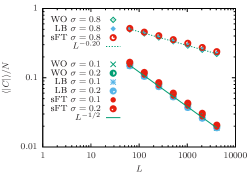
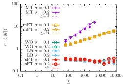
Figure 1: Left: Average relative size $\langle|C|\rangle/N$ of clusters grown in the single-cluster algorithms of the plain Wolff type (WO), the Luijten-Blöte algorithm (LB) and the single-cluster Fukui-Todo update (sFT) for simulations of the 1D long-range critical Ising model at the critical temperature in the non-mean-field ($\sigma=0.8$) and mean-field ($\sigma=0.1$ and $\sigma=0.2$) region of the interaction range. Right: Integrated autocorrelation times of the magnetization for $\sigma=0.1$ and $\sigma=0.2$ in the mean-field regime below the critical value $\sigma=1/2$ for the Metropolis (MT), multi-cluster Fukui-Todo (mFT), Wolff (WO), Luijten-Blöte (LB) and single-cluster Fukui-Todo (sFT) updates as a function of system size $L$.

For the model with power-law interactions, a study of the Langevin dynamics for the spherical model yields $z_{\mathrm{int}}^{\mathrm{Metro}}=\sigma$ cannas:01 . This carries over to the Ising model in the mean-field regime $0<\sigma<1/2$. By analogy to the mean-field limit, we conjecture that $z_{\mathrm{int}}^{\mathrm{SW}}=\sigma/2$ for multi-cluster and $z_{\mathrm{int}}^{\mathrm{Wolff}}=0$ for single-cluster updates in the same regime. Due to the particular scaling of the correlation length with system size according to $\xi\sim L^{\hbox{\footnotesize\coppa}}$ above the upper critical dimension berche:12a , where ${\hbox{\coppa}}=d/d_{c}$ and $d_{c}=4$ for short-range models and ${\hbox{\coppa}}=d/2\sigma$ for the interactions (3) flores:15 , we expect the following finite-size scaling of the autocorrelation times,

$$\tau_{\mathrm{int}}\sim L^{z_{\mathrm{int}}{\hbox{\footnotesize\coppa}}}\sim\left\{\begin{array}[]{l@{\hspace{0.5cm}}l}L^{1/2}\hfil\hskip 14.22636pt&\mbox{for Metropolis},\\ L^{1/4}\hfil\hskip 14.22636pt&\mbox{for multi cluster},\\ L^{0}\hfil\hskip 14.22636pt&\mbox{for single cluster}.\end{array}\right.$$ (14)

We note that this is consistent with the behavior in the limit $\sigma\to 0$, where the model becomes equivalent to a mean-field system, and a scaling $\tau_{\mathrm{int}}\sim L^{z_{\mathrm{int}}/4}$ is observed according to the usual identification of $N^{1/4}$ with the linear system size in the mean-field case persky:96 .

We have determined the integrated autocorrelation times of the energy and magnetization for the 1D power-law model using a standard self-consistent cut-off procedure for the summation of the autocorrelation function given in Eq. (13). For a discussion of this procedure, including the estimation of statistical errors see, e.g., Ref. janke:02 . Our simulations were performed for systems with periodic boundary conditions and for the interaction-range exponents $\sigma=0.1$ and $\sigma=0.2$ in the mean-field range $\sigma<1/2$ as well as a number of values $\sigma\geq 0.5$ in the non-trivial long-range regime. We used an Ewald summed form of the interaction (3) flores:15 and performed simulations at the previously determined critical temperatures $T_{c}=21.0013$ for $\sigma=0.1$, $T_{c}=10.8419$ for $\sigma=0.2$, $T_{c}=4.36395$ for $\sigma=0.5$, $T_{c}=3.54886$ for $\sigma=0.6$, $T_{c}=2.93061$ for $\sigma=0.7$, $T_{c}=2.43267$ for $\sigma=0.8$, and $T_{c}=2.00144$ for $\sigma=0.9$ luijten:97b . To provide autocorrelation times on a common time scale for all algorithms it is convenient to consider updates such that, on average, each spin is touched once (one sweep). While this is automatic for the Metropolis and multi-cluster updates, for the single-cluster variants it implies a rescaling of the raw autocorrelation times $\tau_{\mathrm{int}}^{\prime}$ determined from a time series recorded after each individual single-cluster update according to

$$\tau_{\mathrm{int}}^{\mathrm{sc}}=\tau_{\mathrm{int}}^{\prime}\frac{\langle|C|\rangle}{N},$$

where $\langle|C|\rangle$ denotes the average size of the simulated clusters. It is known that $\langle|C|\rangle$ provides an improved estimator of the susceptibility $\chi$ wj:chem . We hence expect a scaling of $\langle|C|\rangle\sim\xi^{\gamma/\nu}$ and thus $\langle|C|\rangle/N\sim L^{{\hbox{\footnotesize\coppa}}\gamma/\nu-d}$. For the mean-field cases $\sigma=0.1$ and $\sigma=0.2$ the values $\gamma/\nu=\sigma$ flores:15 and ${\hbox{\coppa}}=1/2\sigma$ imply ${\hbox{\footnotesize\coppa}}\gamma/\nu-d=-1/2$. What is more, the long-range model has the pecularity that the value of $\gamma/\nu=2-\eta=\sigma$ does not acquire any corrections beyond mean-field even for $1/2\leq\sigma\leq 1$, such that $\langle|C|\rangle/N$ scales as $L^{\sigma-1}$ there. These theoretical considerations are fully confirmed by the simulation results for the average cluster size summarized in Fig. 1 (left panel).

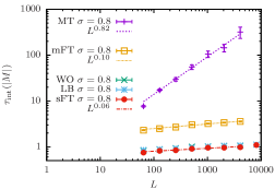
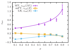
Figure 2: Left: Integrated autocorrelation times for the magnetization for the Metropolis (MT), multi-cluster Fukui-Todo (mFT), Wolff (WO), Luijten-Blöte (LB) and single-cluster Fukui-Todo (sFT) updates at $\sigma=0.8$ in the non-trivial long-range regime. Right: Dynamical critical exponents $z_{\mathrm{int}}$ of the magnetization for the Metropolis update (MT) and of the internal energy for the multi-cluster Fukui-Todo (mFT) and Luijten-Blöte (LB) updates as a function of interaction range $\sigma$. The lines are Bezier curves to guide the eye.

Taking this rescaling into account for the single-cluster variants, the right panel of Fig. 1 shows our numerical results for the integrated autocorrelation times per sweep of the (modulus of the) magnetization for the values $\sigma=0.1$ and $\sigma=0.2$ in the mean-field regime $0\leq\sigma\leq 1/2$. We find excellent agreement with the theoretical prediction (14) with some signs of the presence of scaling corrections for smaller system sizes. In particular, the results confirm that the Wolff algorithm (WO), the Luijten-Blöte algorithm (LB) and the single-cluster variant of the Fukui-Todo update (sFT) introduced here exhibit the same asymptotic dynamical behavior which is substantially superior to the dynamical behavior of the multi-cluster approach (mFT) and, even more so, the Metropolis update (MT). While the data in Fig. 1 show the autocorrelation times of the magnetization, we have also determined those of the internal energy and find practically identical results there (not shown).

Performing similar runs for the non-trivial long-range value $\sigma=0.8$, we arrive at different estimates of $z_{\mathrm{int}}$, cf. the data shown in the left panel of Fig. 2. In this regime we also start to see some differences in the scaling of autocorrelation times for internal energies and magnetizations. It can be shown that for single-spin flip heatbath dynamics the magnetization corresponds to the slowest mode, while for a random-cluster single-bond update (Sweeny’s algorithm sweeny:83 ; elci:13 ) the slowest mode is given by the bond density corresponding to the internal energy elci:15b . We expect the same to be true for the single-spin flip Metropolis update and the various cluster algorithms considered here. We indeed find numerically that our estimates $z_{\mathrm{int}}(|M|)>z_{\mathrm{int}}(E)$ for Metropolis, while in contrast $z_{\mathrm{int}}(|M|)<z_{\mathrm{int}}(E)$ for the cluster updates in the regime $\sigma\geq 0.5$. The right panel of Fig. 2 summarizes our results for $z_{\mathrm{int}}(|M|)$ for Metropolis and $z_{\mathrm{int}}(E)$ for multi-cluster and single-cluster dynamics. Note that the single-cluster algorithms WO, LB and sFT implement the same cluster dynamics, so result in the same estimates of $z_{\mathrm{int}}$, and for clarity we only show one data set. We see that for Metropolis the dynamical critical exponent is moving towards $z_{\mathrm{int}}\gtrsim 2$ expected for short-range models, while the behavior of multi-cluster and single-cluster updates appears to coalesce at a value of $z_{\mathrm{int}}$ close to $0$. We did not perform simulations at the upper critical interaction range $\sigma=1$ as there the system undergoes a Kosterlitz-Thouless phase transition angelini:14 , and we expect strong scaling corrections. For $\sigma>1$ there is no finite-temperature phase transition dyson:69 .

We finally consider the behavior of the actual run-time per update for the different algorithms. While such times are clearly hardware specific, the scaling of the different algorithms is not, and so this is the aspect we focus on here. The left panel of Fig. 3 summarizes the run-times per sweep for the different algorithms run on the same hardware, an Intel Core i5 3210M CPU running at 2.50GHz. The asymptotically quadratic run-times of the MT and WO algorithms are clearly visible. For the LB approach a slightly steeper than linear increase of run-times is seen, but as expected it is difficult to resolve the additional logarithmic component explicitly. The behavior of the mFT approach is compatible with linear scaling in the range of system sizes considered. Finally, the sFT algorithm follows the expected linear scaling in $L$. For the overall efficiency of the considered updates, it is the combination of computational effort per sweep and the achieved integrated autocorrelation times that matters. We hence consider the quantity

$$t_{\mathrm{eff}}=t_{\mathrm{sweep}}\tau_{\mathrm{int}},$$

which is the wall-clock time required to generate a statistically independent sample, as the final measure of efficiency elci:13 . These times are shown in the right panel of Fig. 3 for the algorithms considered here. As the lines in the plot show, the expected scaling from the computational complexity of the algorithms and the dynamical behavior according to Eq. (14) of $\sim L^{2.5}$ for Metropolis, $\sim L^{2}$ for Wolff, $\sim L^{1.25}$ for multi-cluster Fukui-Todo and $\sim L^{1}$ for the single-cluster Fukui-Todo approaches is fully compatible with the numerical data. It is clearly visible that the LB algorithm and the sFT approach introduced here show the asymptotically best performance, with an advantage over the other approaches that grows algebraically with $L$. As the inset displaying the time $t_{\mathrm{eff}}/L$ per spin shows, the sFT approach has perfect linear algorithmic scaling , while the LB algorithm has a logarithmic overhead for the weight look-up. The pronounced step in the run-times of both algorithms is due the fact that at a given, hardware-dependent system size the look-up table starts to exceed the size of the cache memory. At the largest system size considered here, $L=2^{26}\approx 7\times 10^{7}$, the sFT approach is about three times faster than LB. Comparing to the other algorithms, we note that already for $L=65\,536$ the sFT algorithm is about a million times faster to produce an independent sample than the Metropolis method.

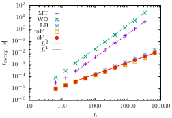
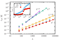
Figure 3: Left: Times in seconds per sweep on an Intel Core i5 3210M CPU for the different update algorithms applied to the 1D long-range Ising model with $\sigma=0.1$ at criticality and fits of the quadratic and linear laws to the data. Right: Time $t_{\mathrm{eff}}$ to generate an effective independent sample of the model with different update algorithms. The inset shows the normalized time $t_{\mathrm{eff}}/L$ per spin comparing the two most efficient approaches, LB and sFT. The legend is the same as that of the plot on the left.

6 Summary and outlook

We have discussed a range of different algorithms for the simulation of spin systems with long-range interactions. Naive approaches exhibit unfavorable $O(N^{2})$ scaling with the number of spins $N$, but it is possible to formulate cluster-update algorithms that combine $O(N\ln N)$ or even $O(N)$ scaling of the run-time per sweep with the additional benefit of a reduced critical slowing down of systems close to continuous phase transitions. The scaling of autocorrelation times in the mean-field regime $0\leq\sigma\leq 1/2$ of the 1D power-law Ising model is explained in terms of the modified QFSS approach to finite-size scaling berche:12a ; flores:15 . We introduced a single-cluster algorithm based on the generalized Fortuin-Kasteleyn representation (9) that is the only known algorithm with strictly linear scaling of run times. It outperforms all previously known approaches and, at the same time, is very straightforward to implement and can be applied to systems in any dimension with or without translational invariance. In the non-trivial long-range regime $1/2\leq\sigma\leq 1$, we observed a continuous variation of dynamical critical exponents with the Metropolis exponent wandering in the direction of the established value $z\gtrsim 2$ expected for short-range models and the values for single-cluster and multi-cluster dynamics coming closer together as the upper critical range $\sigma=1$ is approached.

Some important aspects of the problem have been omitted from the present discussion. This includes the fact that for such systems with periodic boundary conditions a summation over an infinite number of interaction partners is necessary to get reliable results. The corresponding Ewald summation is discussed, e.g., in Refs. flores:15 ; emilio:thesis . Another aspect is the problem of measuring the energy for the long-range interactions, a task that in itself has $O(N^{2})$ scaling in the straightforward approach. As was shown in Ref. fukui:09 , a linear algorithm can be formulated in the framework of the generalized Fortuin-Kasteleyn representation (9). The algorithms discussed here can also be generalized for the presence of external magnetic fields emilio:thesis , but they become less efficient with increasing field strength. While a substantial reduction of critical slowing down from cluster updates can only be expected for non-frustrated systems, the reduction of computational complexity of the present approach as compared to local updates might also make it interesting for simulations of spin-glass systems with long-range interactions beyer:12 .

Author contribution statement

EFS and MW performed the simulations, carried out the analysis and wrote the paper. The paper emerged out of joint work in collaboration with BB and RK.

References

- (1) N. Kawashima and H. Rieger, in Frustrated Spin Systems, edited by H. T. Diep (World Scientific, Singapore, 2005), Chap. 9, p. 491.
- (2) N. G. Fytas, V. Martín-Mayor, M. Picco, and N. Sourlas, Phys. Rev. Lett. 116, 227201 (2016).
- (3) M. Wittmann and A. P. Young, Phys. Rev. E 90, 062137 (2014).
- (4) E. Flores-Sola, B. Berche, R. Kenna, and M. Weigel, Phys. Rev. Lett. 116, 115701 (2016).
- (5) M. E. Fisher, Rev. Mod. Phys. 46, 597 (1974).
- (6) D. C. Rapaport, The Art of Molecular Dynamics Simulation (Cambridge University Press, Cambridge, 2004).
- (7) K. Binder and D. P. Landau, A Guide to Monte Carlo Simulations in Statistical Physics, 4th ed. (Cambridge University Press, Cambridge, 2015).
- (8) N. Metropolis et al., J. Chem. Phys. 21, 1087 (1953).
- (9) R. H. Swendsen and J. S. Wang, Phys. Rev. Lett. 58, 86 (1987).
- (10) U. Wolff, Phys. Rev. Lett. 62, 361 (1989).
- (11) E. Luijten, Lect. Notes Phys. 703, 13 (2006).
- (12) Y. Deng, T. M. Garoni, and A. D. Sokal, Phys. Rev. Lett. 98, 230602 (2007).
- (13) E. M. Elçi and M. Weigel, Phys. Rev. E 88, 033303 (2013).
- (14) C. Lacroix, P. Mendels, and F. Mila, Introduction to Frustrated Magnetism: Materials, Experiments, Theory (Springer, Berlin, 2011), Vol. 164.
- (15) J. W. Britton et al., Nature 484, 489 (2012).
- (16) M. E. Fisher, S. K. Ma, and B. G. Nickel, Phys. Rev. Lett. 29, 917 (1972).
- (17) F. J. Dyson, Commun. Math. Phys. 12, 91 (1969).
- (18) F. J. Dyson, Commun. Math. Phys. 21, 269 (1971).
- (19) H.-J. Xu, B. Bergersen, and Z. Rácz, Phys. Rev. E 47, 1520 (1993).
- (20) J. F. Nagle and J. C. Bonner, J. Phys. C 3, 352 (1970).
- (21) Z. Glumac and K. Uzelac, J. Phys. A 22, 4439 (1989).
- (22) E. Luijten and H. W. Blöte, Int. J. Mod. Phys. C 6, 359 (1995).
- (23) K. Fukui and S. Todo, J. Comp. Phys. 228, 2629 (2009).
- (24) W. Janke, in Computational Physics, edited by K. H. Hoffmann and M. Schreiber (Springer, Berlin, 1996), pp. 10–43.
- (25) C. M. Fortuin and P. W. Kasteleyn, Physica 57, 536 (1972).
- (26) R. G. Edwards and A. D. Sokal, Phys. Rev. D 38, 2009 (1988).
- (27) M. Weigel, Phys. Rev. E 84, 036709 (2011).
- (28) E. Luijten and H. W. J. Blöte, Phys. Rev. B 56, 8945 (1997).
- (29) D. E. Knuth, The Art of Computer Programming, Volume 2: Seminumerical Algorithms, 3rd ed. (Addison-Wesley, Upper Saddle River, NJ, 1997).
- (30) J. E. Gentle, Random number generation and Monte Carlo methods, 2nd ed. (Springer, Berlin, 2003).
- (31) R. E. Tarjan, J. ACM 22, 215 (1975).
- (32) M. E. J. Newman and R. M. Ziff, Phys. Rev. E 64, 016706 (2001).
- (33) W. Janke, in Proceedings of the Euro Winter School “Quantum Simulations of Complex Many-Body Systems: From Theory to Algorithms”, Vol. 10 of NIC Series, edited by J. Grotendorst, D. Marx, and A. Muramatsu (John von Neumann Institute for Computing, Jülich, 2002), pp. 423–445.
- (34) N. Persky, R. Ben-Av, I. Kanter, and E. Domany, Phys. Rev. E 54, 2351 (1996).
- (35) Y. Deng et al., Phys. Rev. Lett. 99, 055701 (2007).
- (36) U. Wolff, Phys. Lett. B 228, 379 (1989).
- (37) T. S. Ray, P. Tamayo, and W. Klein, Phys. Rev. A 39, 5949 (1989).
- (38) S. A. Cannas, D. A. Stariolo, and F. A. Tamarit, Physica A 294, 362 (2001).
- (39) B. Berche, R. Kenna, and J. C. Walter, Nucl. Phys. B 865, 115 (2012).
- (40) E. J. Flores-Sola, B. Berche, R. Kenna, and M. Weigel, Eur. Phys. J. B 88, 1 (2015).
- (41) E. Luijten, Ph.D. thesis, Delft University of Technology, 1997.
- (42) M. Sweeny, Phys. Rev. B 27, 4445 (1983).
- (43) E. M. Elçi, Ph.D. thesis, Coventry University, 2015.
- (44) M. C. Angelini, G. Parisi, and F. Ricci-Tersenghi, Phys. Rev. E 89, 062120 (2014).
- (45) E. Flores-Sola, Ph.D. thesis, Coventry University, Coventry, 2016.
- (46) F. Beyer, M. Weigel, and M. A. Moore, Phys. Rev. B 86, 014431 (2012).