Symmetry, Geometry, and Quantization
with Hypercomplex Numbers

Abstract.

These notes describe some links between the group $\mathrm{SL}_{2}(\mathbb{R}{})$, the Heisenberg group and hypercomplex numbers – complex, dual and double numbers. Relations between quantum and classical mechanics are clarified in this framework. In particular, classical mechanics can be obtained as a theory with noncommutative observables and a non-zero Planck constant if we replace complex numbers in quantum mechanics by dual numbers. Our consideration is based on induced representations which are build from complex-/dual-/double-valued characters. Dynamic equations, rules of additions of probabilities, ladder operators and uncertainty relations are discussed. Finally, we prove a Calderón–Vaillancourt-type norm estimation for relative convolutions.

Introduction

These lecture notes describe some links between the group $\mathrm{SL}_{2}(\mathbb{R}{})$, the Heisenberg group and hypercomplex numbers. The described relations appear in a natural way without any enforcement from our side. The discussion is illustrated by mathematical models of various physical systems.

By hypercomplex numbers we mean two-dimensional real associative commutative algebras. It is known [LavrentShabat77], that any such algebra is isomorphic either to complex, dual or double numbers, that is collection of elements $a+\iota b$, where $a$, $b\in\mathbb{R}{}$ and $\iota^{2}=-1$, $0$ or $1$. Complex numbers are crucial in quantum mechanics (or, in fact, any wave process), dual numbers similarly serve classical mechanics and double numbers are perfect to encode relativistic space-time.

Section 1 contains an easy-reading overview of the rôle of complex numbers in quantum mechanics and indicates that classical mechanics can be described as a theory with noncommutative observables and a non-zero Planck constant if we replace complex numbers by dual numbers. The Heisenberg group is the main ingredient for both – quantum and classic – models. The detailed exposition of the theory is provided in the following sections.

Section 2 introduces the group $\mathrm{SL}_{2}(\mathbb{R}{})$ and describes all its actions on two-dimensional homogeneous spaces: it turns out that they are Möbius transformations of complex, dual and double numbers. We also re-introduce the Heisenberg group in more details. In particular, we point out Heisenberg group’s automorphisms from the symplectic action of $\mathrm{SL}_{2}(\mathbb{R}{})$.

Section 3 uses Mackey’s induced representation to construct linear representations of $\mathrm{SL}_{2}(\mathbb{R}{})$ and the Heisenberg group. We use all sorts (complex, dual and double) of characters of one-dimensional subgroups to induce representations of $\mathrm{SL}_{2}(\mathbb{R}{})$. The similarity between obtained representations in hypercomplex numbers is illustrated by corresponding ladder operators.

Section 4 systematically presents the Hamiltonian formalism obtained from linear representations of the Heisenberg group. Using complex, dual and double numbers we recover principal elements of quantum, classical and hyperbolic (relativistic?) mechanics. This includes both the Hamilton–Heisenberg dynamical equation, rules of addition of probabilities and some examples.

Section 5 introduces co- and contra-variant transforms, which are also known under many other names, e.g. wavelet transform. These transforms intertwine the given representation with left and right regular representations. We use this observation to derive a connection between the uncertainty relations and analyticity condition – both in the standard meaning for the Heisenberg group and a new one for $\mathrm{SL}_{2}(\mathbb{R}{})$. We also obtain a Calderón–Vaillancourt-type norm estimation for integrated representation.

1. Preview: Quantum and Classical Mechanics

…it was on a Sunday that the idea first occurred to me that $ab-ba$ might correspond to a Poisson bracket.

P.A.M. Dirac, http://www.aip.org/history/ohilist/4575_1.html

In this section we will demonstrate that a Poisson bracket do not only corresponds to a commutator, in fact a Poisson bracket is the image of the commutator under a transformation which uses dual numbers.

1.1. Axioms of Mechanics

There is a recent revival of interest in foundations of quantum mechanics, which is essentially motivated by engineering challenges at the nano-scale. There are strong indications that we need to revise the development of the quantum theory from its early days.

In 1926, Dirac discussed the idea that quantum mechanics can be obtained from classical description through a change in the only rule, cf. [Dirac26a]:

…there is one basic assumption of the classical theory which is false, and that if this assumption were removed and replaced by something more general, the whole of atomic theory would follow quite naturally. Until quite recently, however, one has had no idea of what this assumption could be.

In Dirac’s view, such a condition is provided by the Heisenberg commutation relation of coordinate and momentum variables [Dirac26a]*(1):

(1) $$q_{r}p_{r}-p_{r}q_{r}=\mathrm{i}h.$$

Algebraically, this identity declares noncommutativity of $q_{r}$ and $p_{r}$. Thus, Dirac stated [Dirac26a] that classical mechanics is formulated through commutative quantities (“c-numbers” in his terms) while quantum mechanics requires noncommutative quantities (“q-numbers”). The rest of theory may be unchanged if it does not contradict to the above algebraic rules. This was explicitly re-affirmed at the first sentence of the subsequent paper [Dirac26b]:

The new mechanics of the atom introduced by Heisenberg may be based on the assumption that the variables that describe a dynamical system do not obey the commutative law of multiplication, but satisfy instead certain quantum conditions.

The same point of view is expressed in his later works [DiracDirections]*p. 6[DiracPrinciplesQM]*p. 26.

Dirac’s approach was largely approved, especially by researchers on the mathematical side of the board. Moreover, the vague version – “quantum is something noncommutative” – of the original statement was lightly reverted to “everything noncommutative is quantum”. For example, there is a fashion to label any noncommutative algebra as a “quantum space” [Cuntz01a].

Let us carefully review Dirac’s idea about noncommutativity as the principal source of quantum theory.

1.2. “Algebra” of Observables

Dropping the commutativity hypothesis on observables, Dirac made [Dirac26a] the following (apparently flexible) assumption:

All one knows about q-numbers is that if $z_{1}$ and $z_{2}$ are two q-numbers, or one q-number and one c-number, there exist the numbers $z_{1}+z_{2}$, $z_{1}z_{2}$, $z_{2}z_{1}$, which will in general be q-numbers but may be c-numbers.

Mathematically, this (together with some natural identities) means that observables form an algebraic structure known as a ring. Furthermore, the linear superposition principle imposes a liner structure upon observables, thus their set becomes an algebra. Some mathematically-oriented texts, e.g. [FaddeevYakubovskii09]*§ 1.2, directly speak about an “algebra of observables” which is not far from the above quote [Dirac26a]. It is also deducible from two connected statements in Dirac’s canonical textbook:

1. “the linear operators corresponds to the dynamical variables at that time” [DiracPrinciplesQM]*§ 7, p. 26.

2. “Linear operators can be added together” [DiracPrinciplesQM]*§ 7, p. 23.

However, the assumption that any two observables may be added cannot fit into a physical theory. To admit addition, observables need to have the same dimensionality. In the simplest example of the observables of coordinate $q$ and momentum $p$, which units shall be assigned to the expression $q+p$? Meters or $\frac{\text{kilos}\times\text{meters}}{\text{seconds}}$? If we get the value $5$ for $p+q$ in the metric units, what is then the result in the imperial ones? Since these questions cannot be answered, the above Dirac’s assumption is not a part of any physical theory.

Another common definition suffering from the same problem is used in many excellent books written by distinguished mathematicians, see for example [Mackey63]*§ 2-2 [Folland89]*§ 1.1. It declares that quantum observables are projection-valued Borel measures on the dimensionless real line. Such a definition permit an instant construction (through the functional calculus) of new observables, including algebraically formed [Mackey63]*§ 2-2, p. 63:

Because of Axiom III, expressions such as $A^{2}$, $A^{3}+A$, $1-A$, and $\mathrm{e}^{A}$ all make sense whenever $A$ is an observable.

However, if $A$ has a physical dimension (is not a scalar) then the expression $A^{3}+A$ cannot be assigned a dimension in a consistent manner.

Of course, physical defects of the above (otherwise perfect) mathematical constructions do not prevent physicists from making correct calculations, which are in a good agreement with experiments. We are not going to analyse methods which allow researchers to escape the indicated dangers. Instead, it will be more beneficial to outline alternative mathematical foundations of quantum theory, which do not have those shortcomings.

1.3. Non-Essential Noncommutativity

While we can add two observables if they have the same dimension only, physics allows us to multiply any observables freely. Of course, the dimensionality of a product is the product of dimensionalities, thus the commutator $[A,B]=AB-BA$ is well defined for any two observables $A$ and $B$. In particular, the commutator (1) is also well-defined, but is it indeed so important?

In fact, it is easy to argue that noncommutativity of observables is not an essential prerequisite for quantum mechanics: there are constructions of quantum theory which do not relay on it at all. The most prominent example is the Feynman path integral. To focus on the really cardinal moments, we firstly take the popular lectures [Feynman1990qed], which present the main elements in a very enlightening way. Feynman managed to tell the fundamental features of quantum electrodynamics without any reference to (non-)commutativity: the entire text does not mention it anywhere.

Is this an artefact of the popular nature of these lecture? Take the academic presentation of path integral technique given in [FeynHibbs65]. It mentioned (non-)commutativity only on pages 115–6 and 176. In addition, page 355 contains a remark on noncommutativity of quaternions, which is irrelevant to our topic. Moreover, page 176 highlights that noncommutativity of quantum observables is a consequence of the path integral formalism rather than an indispensable axiom.

But what is the mathematical source of quantum theory if noncommutativity is not? The vivid presentation in [Feynman1990qed] uses stopwatch with a single hand to explain the calculation of path integrals. The angle of stopwatch’s hand presents the phase for a path $x(t)$ between two points in the configuration space. The mathematical expression for the path’s phase is [FeynHibbs65]*(2-15):

(2) $$\phi[x(t)]=\mathrm{const}\cdot\mathrm{e}^{(\mathrm{i}/\hslash)S[x(t)]}$$

where $S[x(t)]$ is the classic action along the path $x(t)$. Summing up contributions (2) along all paths between two points $a$ and $b$ we obtain the amplitude $K(a,b)$. This amplitude presents very accurate description of many quantum phenomena. Therefore, expression (2) is also a strong contestant for the rôle of the cornerstone of quantum theory.

Is there anything common between two “principal” identities (1) and (2)? Seemingly, not. A more attentive reader may say that there are only two common elements there (in order of believed significance):

1. The non-zero Planck constant $\hslash$.

2. The imaginary unit $\mathrm{i}$.

The Planck constant was the first manifestation of quantum (discrete) behaviour and it is at the heart of the whole theory. In contrast, classical mechanics is oftenly obtained as a semiclassical limit $\hslash\rightarrow 0$. Thus, the non-zero Planck constant looks like a clear marker of quantum world in its opposition to the classical one. Regrettably, there is a common practice to “chose our units such that $\hslash=1$”. Thus, the Planck constant becomes oftenly invisible in many formulae even being implicitly present there. Note also, that $1$ in the identity $\hslash=1$ is not a scalar but a physical quantity with the dimensionality of the action. Thus, the simple omission of the Planck constant invalidates dimensionalities of physical equations.

The complex imaginary unit is also a mandatory element of quantum mechanics in all its possible formulations. It is enough to point out that the popular lectures [Feynman1990qed] managed to avoid any mention of noncommutativity but did uses complex numbers both explicitly (see the Index there) and implicitly (as rotations of the hand of a stopwatch). However, it is a common perception that complex numbers are a useful but manly technical tool in quantum theory.

1.4. Quantum Mechanics from the Heisenberg Group

Looking for a source of quantum theory we again return to the Heisenberg commutation relations (1): they are an important part of quantum mechanics (either as a prerequisite or as a consequence). It was observed for a long time that these relations are a representation of the structural identities of the Lie algebra of the Heisenberg group [Folland89, Howe80a, Howe80b]. In the simplest case of one dimension, the Heisenberg group $\mathbb{H}{}=\mathbb{H}^{1}{}$ can be realised by the Euclidean space $\mathbb{R}^{3}{}$ with the group law:

(3) $$\textstyle(s,x,y)*(s^{\prime},x^{\prime},y^{\prime})=(s+s^{\prime}+\frac{1}{2}\omega(x,y;x^{\prime},y^{\prime}),x+x^{\prime},y+y^{\prime})$$

where $\omega$ is the symplectic form on $\mathbb{R}^{2}{}$ [Arnold91]*§ 37, which is behind the entire classical Hamiltonian formalism:

(4) $$\omega(x,y;x^{\prime},y^{\prime})=xy^{\prime}-x^{\prime}y.$$

Here, like for the path integral, we see another example of a quantum notion being defined through a classical object.

The Heisenberg group is noncommutative since $\omega(x,y;x^{\prime},y^{\prime})=-\omega(x^{\prime},y^{\prime};x,y)$. The collection of points $(s,0,0)$ forms the centre of $\mathbb{H}{}$, that is $(s,0,0)$ commutes with any other element of the group. We are interested in the unitary irreducible representations (UIRs) ${\rho}$ of $\mathbb{H}{}$ in an infinite-dimensional Hilbert space $H$, that is a group homomorphism (${\rho}(g_{1}){\rho}(g_{2})={\rho}(g_{1}*g_{2})$) from $\mathbb{H}{}$ to unitary operators on $H$. By Schur’s lemma, for such a representation ${\rho}$, the action of the centre shall be multiplication by an unimodular complex number, i.e. ${\rho}(s,0,0)=\mathrm{e}^{2\pi\mathrm{i}\hslash s}I$ for some real $\hslash\neq 0$.

Furthermore, the celebrated Stone–von Neumann theorem [Folland89]*§ 1.5 tells that all UIRs of $\mathbb{H}{}$ in complex Hilbert spaces with the same value of $\hslash$ are unitary equivalent. In particular, this implies that any realisation of quantum mechanics, e.g. the Schrödinger wave mechanics, which provides the commutation relations (1) shall be unitary equivalent to the Heisenberg matrix mechanics based on these relations.

In particular, any UIR of $\mathbb{H}{}$ is equivalent to a subrepresentation of the following representation on $\mathcal{L}_{2}{}(\mathbb{R}^{2}{})$:

(5) $$\textstyle{\rho_{\hslash}}(s,x,y):f(q,p)\mapsto\mathrm{e}^{-2\pi\mathrm{i}(\hslash s+qx+py)}f\left(q-\frac{\hslash}{2}y,p+\frac{\hslash}{2}x\right).$$

Here $\mathbb{R}^{2}{}$ has the physical meaning of the classical phase space with $q$ representing the coordinate in the configurational space and $p$—the respective momentum. The function $f(q,p)$ in (5) presents a state of the physical system as an amplitude over the phase space. Thus, the action (5) is more intuitive and has many technical advantages [Howe80b, Zachos02a, Folland89] in comparison with the well-known Schrödinger representation (cf. (78)), to which it is unitary equivalent, of course.

Infinitesimal generators of the one-parameter subgroups ${\rho_{\hslash}}(0,x,0)$ and ${\rho_{\hslash}}(0,0,y)$ from (5) are the operators $\frac{1}{2}\hslash\partial_{p}-2\pi\mathrm{i}q$ and $-\frac{1}{2}\hslash\partial_{q}-2\pi\mathrm{i}p$. For these, we can directly verify the commutator identity:

$$\textstyle[-\frac{1}{2}\hslash\partial_{q}-2\pi\mathrm{i}p,\frac{1}{2}\hslash\partial_{p}-2\pi\mathrm{i}q]=\mathrm{i}h,\quad\text{ where }h=2\pi\hslash.$$

Since we have a representation of (1), these operators can be used as a model of the quantum coordinate and momentum.

For a Hamiltonian $H(q,p)$ we can integrate the representation ${\rho_{\hslash}}$ with the Fourier transform $\hat{H}(x,y)$ of $H(q,p)$:

(6) $$\tilde{H}=\int_{\mathbb{R}^{2}{}}\hat{H}(x,y)\,{\rho_{\hslash}}(0,x,y)\,\mathrm{d}x\,\mathrm{d}y$$

and obtain (possibly unbounded) operator $\tilde{H}$ on $\mathcal{L}_{2}{}(\mathbb{R}^{2}{})$. This assignment of the operator $\tilde{H}$ (quantum observable) to a function $H(q,p)$ (classical observable) is known as the Weyl quantization or a Weyl calculus [Folland89]*§ 2.1. The Hamiltonian $\tilde{H}$ defines the dynamics of a quantum observable $\tilde{k}$ by the Heisenberg equation:

(7) $$\mathrm{i}h\frac{\mathrm{d}\tilde{k}}{\mathrm{d}t}=\tilde{H}\tilde{k}-\tilde{k}\tilde{H}.$$

This is sketch of the well-known construction of quantum mechanics from infinite-dimensional UIRs of the Heisenberg group, which can be found in numerous sources [Kisil02e, Folland89, Howe80b].

1.5. Classical Noncommutativity

Now we are going to show that the priority of importance in quantum theory shall be shifted from the Planck constant towards the imaginary unit. Namely, we describe a model of classical mechanics with a non-zero Planck constant but with a different hypercomplex unit. Instead of the imaginary unit with the property $\mathrm{i}^{2}=-1$ we will use the nilpotent unit $\varepsilon$ such that $\varepsilon^{2}=0$. The dual numbers generated by nilpotent unit were already known for there connections with Galilean relativity [Yaglom79, Gromov90a] – the fundamental symmetry of classical mechanics – thus its appearance in our discussion shall not be very surprising after all. Rather, we may wander why the following construction was unnoticed for such a long time.

Another important feature of our scheme is that the classical mechanics is presented by a noncommutative model. Therefore, it will be a refutation of Dirac’s claim about the exclusive rôle of noncommutativity for quantum theory. Moreover, the model is developed from the same Heisenberg group, which were used above to describe the quantum mechanics.

Consider a four-dimensional algebra $\mathfrak{C}$ spanned by $1$, $\mathrm{i}$, $\varepsilon$ and $\mathrm{i}\varepsilon$. We can define the following representation ${\rho_{\varepsilon h}}$ of the Heisenberg group in a space of $\mathfrak{C}$-valued smooth functions [Kisil10a, Kisil11c]:

$${\rho_{\varepsilon h}}(s,x,y):\ f(q,p)\mapsto$$

$$\mathrm{e}^{-2\pi\mathrm{i}(xq+yp)}\left(f(q,p)+\varepsilon\hbar\left(2\pi sf(q,p)-\frac{\mathrm{i}y}{2}f^{\prime}_{q}(q,p)+\frac{\mathrm{i}x}{2}f^{\prime}_{p}(q,p)\right)\right).$$

A simple calculation shows the representation property

$${\rho_{\varepsilon h}}(s,x,y){\rho_{\varepsilon h}}(s^{\prime},x^{\prime},y^{\prime})={\rho_{\varepsilon h}}((s,x,y)*(s^{\prime},x^{\prime},y^{\prime}))$$

for the multiplication (3) on $\mathbb{H}{}$. Since this is not a unitary representation in a complex-valued Hilbert space its existence does not contradict the Stone–von Neumann theorem. Both representations (5) and (1.5) are noncommutative and act on functions over the phase space. The important distinction is:

• The representation (5) is induced (in the sense of Mackey [Kirillov76]*§ 13.4) by the complex-valued unitary character ${\rho_{\hslash}}(s,0,0)=\mathrm{e}^{2\pi\mathrm{i}\hslash s}$ of the centre of $\mathbb{H}{}$.

• The representation (1.5) is similarly induced by the dual number-valued character ${\rho_{\varepsilon h}}(s,0,0)=\mathrm{e}^{\varepsilon hs}=1+\varepsilon hs$ of the centre of $\mathbb{H}{}$, cf. [Kisil09c]. Here dual numbers are the associative and commutative two-dimensional algebra spanned by $1$ and $\varepsilon$.

Similarity between (5) and (1.5) is even more striking if (1.5) is written as:

(9) $${\rho_{\hslash}}(s,x,y):f(q,p)\mapsto\mathrm{e}^{-2\pi(\varepsilon\hslash s+\mathrm{i}(qx+py))}f\left(q-\frac{\mathrm{i}\hslash}{2}\varepsilon y,p+\frac{\mathrm{i}\hslash}{2}\varepsilon x\right).$$

Here, for a differentiable function $k$ of a real variable $t$, the expression $k(t+\varepsilon a)$ is understood as $k(t)+\varepsilon ak^{\prime}(t)$, where $a\in\mathbb{C}{}$ is a constant. For a real-analytic function $k$ this can be justified through its Taylor’s expansion, see [CatoniCannataNichelatti04] [Zejliger34]*§ I.2(10) [Gromov90a] [Dimentberg78a] [Dimentberg78b]. The same expression appears within the non-standard analysis based on the idempotent unit $\varepsilon$ [Bell08a].

The infinitesimal generators of one-parameter subgroups ${\rho_{\varepsilon h}}(0,x,0)$ and ${\rho_{\varepsilon h}}(0,0,y)$ in (1.5) are

$$\mathrm{d}{\rho^{X}_{\varepsilon h}}=-2\pi\mathrm{i}q-\frac{\varepsilon h}{4\pi\mathrm{i}}\partial_{p}\quad\text{ and }\quad\mathrm{d}{\rho^{Y}_{\varepsilon h}}=-2\pi\mathrm{i}p+\frac{\varepsilon h}{4\pi\mathrm{i}}\partial_{q},$$

respectively. We calculate their commutator:

(10) $$\mathrm{d}{\rho^{X}_{\varepsilon h}}\cdot\mathrm{d}{\rho^{Y}_{\varepsilon h}}-\mathrm{d}{\rho^{Y}_{\varepsilon h}}\cdot\mathrm{d}{\rho^{X}_{\varepsilon h}}=\varepsilon h.$$

It is similar to the Heisenberg relation (1): the commutator is non-zero and is proportional to the Planck constant. The only difference is the replacement of the imaginary unit by the nilpotent one. The radical nature of this change becomes clear if we integrate this representation with the Fourier transform $\hat{H}(x,y)$ of a Hamiltonian function $H(q,p)$:

(11) $$\mathring{H}=\int_{\mathbb{R}^{2n}{}}\hat{H}(x,y)\,{\rho_{\varepsilon h}}(0,x,y)\,\mathrm{d}x\,\mathrm{d}y=H+\frac{\varepsilon h}{2}\left(\frac{\partial H}{\partial p}\frac{\partial\ }{\partial q}-\frac{\partial H}{\partial q}\frac{\partial\ }{\partial p}\right).$$

This is a first order differential operator on the phase space. It generates a dynamics of a classical observable $k$ – a smooth real-valued function on the phase space – through the equation isomorphic to the Heisenberg equation (7):

$$\varepsilon h\frac{\mathrm{d}\mathring{k}}{\mathrm{d}t}=\mathring{H}\mathring{k}-\mathring{k}\mathring{H}.$$

Making a substitution from (11) and using the identity $\varepsilon^{2}=0$ we obtain:

(12) $$\frac{\mathrm{d}{k}}{\mathrm{d}t}=\frac{\partial H}{\partial p}\frac{\partial k}{\partial q}-\frac{\partial H}{\partial q}\frac{\partial k}{\partial p}\,.$$

This is, of course, the Hamilton equation of classical mechanics based on the Poisson bracket. Dirac suggested, see the paper’s epigraph, that the commutator corresponds to the Poisson bracket. However, the commutator in the representation (1.5) is exactly the Poisson bracket.

Note also, that both the Planck constant and the nilpotent unit disappeared from (12), however we did use the fact $h\neq 0$ to make this cancellation. Also, the shy disappearance of the nilpotent unit $\varepsilon$ at the very last minute can explain why its rôle remain unnoticed for a long time.

1.6. Summary

We revised mathematical foundations of quantum and classical mechanics and the rôle of hypercomplex units $\mathrm{i}^{2}=-1$ and $\varepsilon^{2}=0$ there. To make the consideration complete, one may wish to consider the third logical possibility of the hyperbolic unit $\mathrm{j}$ with the property $\mathrm{j}^{2}=1$ [Hudson66a, Khrennikov09book, Kisil10a, Ulrych10a, Pilipchuk10a, Kisil12a, Kisil09c], see Section 4.4.

The above discussion provides the following observations [Kisil12c]:

1. Noncommutativity is not a crucial prerequisite for quantum theory, it can be obtained as a consequence of other fundamental assumptions.

2. Noncommutativity is not a distinguished feature of quantum theory, there are noncommutative formulations of classical mechanics as well.

3. The non-zero Planck constant is compatible with classical mechanics. Thus, there is no a necessity to consider the semiclassical limit $\hslash\rightarrow 0$, where the constant has to tend to zero.

4. There is no a necessity to request that physical observables form an algebra, which is a physical non-sense since we cannot add two observables of different dimensionalities. Quantization can be performed by the Weyl recipe, which requires only a structure of a linear space in the collection of all observables with the same physical dimensionality.

5. It is the imaginary unit in (1), which is ultimately responsible for most of quantum effects. Classical mechanics can be obtained from the similar commutator relation (10) using the nilpotent unit $\varepsilon^{2}=0$.

In Dirac’s opinion, quantum noncommutativity was so important because it guaranties a non-trivial commutator, which is required to substitute the Poisson bracket. In our model, multiplication of classical observables is also non-commutative and the Poisson bracket exactly is the commutator. Thus, these elements do not separate quantum and classical models anymore.

Our consideration illustrates the following statement on the exceptional rôle of the complex numbers in quantum theory [Penrose78a]:

…for the first time, the complex field $\mathbb{C}$ was brought into physics at a fundamental and universal level, not just as a useful or elegant device, as had often been the case earlier for many applications of complex numbers to physics, but at the very basis of physical law.

Thus, Dirac may be right that we need to change a single assumption to get a transition between classical mechanics and quantum. But, it shall not be a move from commutative to noncommutative. Instead, we need to replace a representation of the Heisenberg group induced from a dual number-valued character by the representation induced by a complex-valued character. Our conclusion can be stated like a proportionality:

Classical$/$Quantum$=$Dual numbers$/$Complex numbers.

2. Groups, Homogeneous Spaces and Hypercomplex Numbers

This section shows that the group $\mathrm{SL}_{2}(\mathbb{R}{})$ naturally requires complex, dual and double numbers to describe its action on homogeneous space. And the group $\mathrm{SL}_{2}(\mathbb{R}{})$ acts by automorphism on the Heisenberg group, thus the Heisenberg group is naturally linked to hypercomplex numbers as well.

2.1. The Group $\mathrm{SL}_{2}(\mathbb{R}{})$ and Its Subgroups

The $\mathrm{SL}_{2}(\mathbb{R}{})$ group [Lang85] consists of $2\times 2$ real matrices with unit determinant. This is the smallest semis-simple Lie group, its Lie algebra is formed by zero-trace $2\times 2$ real matrices. The $ax+b$ group, which is used wavelet theory and harmonic analysis [Kisil12d], is only a subgroup of $\mathrm{SL}_{2}(\mathbb{R}{})$ consisting of the upper-triangular matrices $\begin{pmatrix}a^{1/2}&b\\ 0&a^{-1/2}\end{pmatrix}$.

Consider the Lie algebra $\mathfrak{sl}_{2}$ of the group $\mathrm{SL}_{2}(\mathbb{R}{})$. Pick up the following basis in $\mathfrak{sl}_{2}$ [MTaylor86]*§ 8.1:

(13) $$A=\frac{1}{2}\begin{pmatrix}-1&0\\ 0&1\end{pmatrix},\quad B=\frac{1}{2}\ \begin{pmatrix}0&1\\ 1&0\end{pmatrix},\quad Z=\begin{pmatrix}0&1\\ -1&0\end{pmatrix}.$$

The commutation relations between the elements are:

(14) $$[Z,A]=2B,\qquad[Z,B]=-2A,\qquad[A,B]=-\frac{1}{2}Z.$$

Any element $X$ of the Lie algebra $\mathfrak{sl}_{2}$ defines a one-parameter continuous subgroup $A(t)$ of $\mathrm{SL}_{2}(\mathbb{R}{})$ through the exponentiation: $A(t)=\exp(tX)$. There are only three different types of such subgroups under the matrix similarity $A(t)\mapsto MA(t)M^{-1}$ for some constant $M\in\mathrm{SL}_{2}(\mathbb{R}{})$.

Proposition 2.1.

Any continuous one-parameter subgroup of $\mathrm{SL}_{2}(\mathbb{R}{})$ is conjugate to one of the following subgroups:

(15) $$A = \left\{\begin{pmatrix}\mathrm{e}^{-t/2}&0\\ 0&\mathrm{e}^{t/2}\end{pmatrix}=\exp\begin{pmatrix}-t/2&0\\ 0&t/2\end{pmatrix},\ t\in\mathbb{R}{}\right\},$$

(16) $$N = \left\{{\begin{pmatrix}1&t\\ 0&1\end{pmatrix}=\exp\begin{pmatrix}0&t\\ 0&0\end{pmatrix},}\ t\in\mathbb{R}{}\right\},$$

(17) $$K = \left\{{\begin{pmatrix}\cos t&\sin t\\ -\sin t&\cos t\end{pmatrix}=\exp\begin{pmatrix}0&t\\ -t&0\end{pmatrix}},\ t\in(-\pi,\pi]\right\}.$$

2.2. Action of $\mathrm{SL}_{2}(\mathbb{R}{})$ as a Source of Hypercomplex Numbers

We recall the following standard construction [Kirillov76]*§ 13.2. Let $H$ be a closed subgroup of a Lie group $G$. Let $\Omega=G/H$ be the corresponding homogeneous space and $s:\Omega\rightarrow G$ be a smooth section, which is a right inverse to the natural projection $p:G\rightarrow\Omega$. The choice of $s$ is inessential in the sense that by a smooth map $\Omega\rightarrow\Omega$ we can always reduce one to another.

Any $g\in G$ has a unique decomposition of the form $g=s(\omega)h$, where $\omega=p(g)\in\Omega$ and $h\in H$. Note that $\Omega$ is a left homogeneous space with the $G$-action defined in terms of $p$ and $s$ as follows:

(18) $$g:\omega\mapsto g\cdot\omega=p(g*s(\omega))$$

where $*$ is the multiplication on $G$. This is also illustrated by the following commutative diagram:

We want to describe homogeneous spaces obtained from $G=\mathrm{SL}_{2}(\mathbb{R}{})$ and $H$ be one-dimensional continuous subgroup of $\mathrm{SL}_{2}(\mathbb{R}{})$. For $G=\mathrm{SL}_{2}(\mathbb{R}{})$, as well as for other semisimple groups, it is common to consider only the case of $H$ being the maximal compact subgroup $K$. However, in this paper we admit $H$ to be any one-dimensional continuous subgroup. Due to Prop. 2.1 it is sufficient to take $H=K$, $N$ or $A$. Then $\Omega$ is a two-dimensional manifold and for any choice of $H$ we define [Kisil97c]*Ex. 3.7(a):

(19) $$s:(u,v)\mapsto\frac{1}{\sqrt{v}}\begin{pmatrix}v&u\\ 0&1\end{pmatrix},\qquad(u,v)\in\mathbb{R}^{2}{},\ v>0.$$

A direct (or computer algebra [Kisil07a]) calculation show that:

Proposition 2.2.

The $\mathrm{SL}_{2}(\mathbb{R}{})$ action (18) associated to the map $s$ (19) is:

(20) $$\begin{pmatrix}a&b\\ c&d\end{pmatrix}:(u,v)\mapsto\left(\frac{(au+b)(cu+d)-\sigma cav^{2}}{(cu+d)^{2}-\sigma(cv)^{2}},\frac{v}{(cu+d)^{2}-\sigma(cv)^{2}}\right)$$

where $\sigma=-1$, $0$ and $1$ for the subgroups $K$, $N^{\prime}$ and $A^{\prime}$ respectively.

The expression in (20) does not look very appealing, however an introduction of hypercomplex numbers makes it more attractive:

Proposition 2.3.

Let a hypercomplex unit $\iota$ be such that $\iota^{2}=\sigma$, then the $\mathrm{SL}_{2}(\mathbb{R}{})$ action (20) becomes:

(21) $$\begin{pmatrix}a&b\\ c&d\end{pmatrix}:w\mapsto\frac{aw+b}{cw+d},\qquad\text{where }w=u+\iota v$$

for all three cases parametrised by $\sigma$ as in Prop. 2.2.

Remark 2.4.

We wish to stress that the hypercomplex numbers were not introduced here by our intention, arbitrariness or “generalising attitude” [Pontryagin86a]*p. 4. They were naturally created by the $\mathrm{SL}_{2}(\mathbb{R}{})$ action.

Notably the action (21) is a group homomorphism of the group $\mathrm{SL}_{2}(\mathbb{R}{})$ into transformations of the “upper half-plane” on hypercomplex numbers. Although dual and double numbers are algebraically trivial, the respective geometries in the spirit of Erlangen programme are refreshingly inspiring [Kisil05a, Kisil12a, Kisil08a] and provide useful insights even in the elliptic case [Kisil06a]. In order to treat divisors of zero, we need to consider Möbius transformations (21) of conformally completed plane [HerranzSantander02b, Kisil06b].

The arithmetic of dual and double numbers is different from complex numbers mainly in the following aspects:

1. They have zero divisors. However, we are still able to define their transforms by (21) in most cases. The proper treatment of zero divisors will be done through corresponding compactification [Kisil12a]*§ 8.1.

2. They are not algebraically closed. However, this property of complex numbers is not used very often in analysis.

Three possible values $-1$, $0$ and $1$ of $\sigma:=\iota^{2}$ will be referred to here as elliptic, parabolic and hyperbolic cases, respectively. This separation into three cases will be referred to as the EPH classification. Unfortunately, there is a clash here with the already established label for the Lobachevsky geometry. It is often called hyperbolic geometry because it can be realised as a Riemann geometry on a two-sheet hyperboloid. However, within our framework, the Lobachevsky geometry should be called elliptic and it will have a true hyperbolic counterpart.

Notation 2.5.

We denote the space $\mathbb{R}^{2}{}$ of vectors $u+v\iota$ by $\mathbb{R}_{e}{}$, $\mathbb{R}_{p}{}$ or $\mathbb{R}_{h}{}$ to highlight which number system (complex, dual or double, respectively) is used. The notation $\mathbb{R}_{\sigma}{}$ is used for a generic case.

2.3. Orbits of the Subgroup Actions

We start our investigation of the Möbius transformations (21)

$$\begin{pmatrix}a&b\\ c&d\end{pmatrix}:\ w\mapsto\frac{aw+b}{cw+d}$$

on the hypercomplex numbers $w=u+\iota v$ from a description of orbits produced by the subgroups $A^{\prime}$, $N^{\prime}$ and $K$. Due to the Iwasawa decomposition $\mathrm{SL}_{2}(\mathbb{R}{})=ANK$, any Möbius transformation can be represented as a superposition of these three actions.

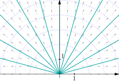
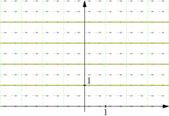
Figure 1. Actions of the subgroups $A$ and $N$ by Möbius transformations. Transverse thin lines are images of the vertical axis, grey arrows show the derived action.

The actions of subgroups $A$ and $N$ for any kind of hypercomplex numbers on the plane are the same as on the real line: $A$ dilates and $N$ shifts – see Fig. 1 for illustrations. Thin traversal lines in Fig. 1 join points of orbits obtained from the vertical axis by the same values of $t$ and grey arrows represent “local velocities” – vector fields of derived representations.

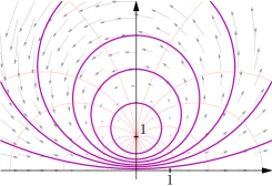
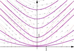
Figure 2. Action of the subgroup $K$. The corresponding orbits are circles, parabolas and hyperbolas shown by thick lines. Transverse thin lines are images of the vertical axis, grey arrows show the derived action.

By contrast, the action of the third matrix from the subgroup $K$ sharply depends on $\sigma=\iota^{2}$, as illustrated by Fig. 2. In elliptic, parabolic and hyperbolic cases, $K$-orbits are circles, parabolas and (equilateral) hyperbolas, respectively. The meaning of traversal lines and vector fields is the same as on the previous figure.

At the beginning of this subsection we described how subgroups generate homogeneous spaces. The following exercise goes it in the opposite way: from the group action on a homogeneous space to the corresponding subgroup, which fixes the certain point.

Exercise 2.6.

Let $\mathrm{SL}_{2}(\mathbb{R}{})$ act by Möbius transformations (21) on the three number systems. Show that the isotropy subgroups of the point $\iota$ are:

1. The subgroup $K$ in the elliptic case. Thus, the elliptic upper half-plane is a model for the homogeneous space $\mathrm{SL}_{2}(\mathbb{R}{})/K$.

2. The subgroup $N^{\prime}$ (22) of matrices

   (22) $$\begin{pmatrix}1&0\\ \nu&1\end{pmatrix}=\begin{pmatrix}0&-1\\ 1&0\end{pmatrix}\begin{pmatrix}1&\nu\\ 0&1\end{pmatrix}\begin{pmatrix}0&1\\ -1&0\end{pmatrix}$$

   in the parabolic case. It also fixes any point $\varepsilon v$ on the vertical axis, which is the set of zero divisors in dual numbers. The subgroup $N^{\prime}$ is conjugate to subgroup $N$, thus the parabolic upper half-plane is a model for the homogeneous space $\mathrm{SL}_{2}(\mathbb{R}{})/N$.

3. The subgroup $A^{\prime}$ (23) of matrices

   (23) $$\begin{pmatrix}\cosh\tau&\sinh\tau\\ \sinh\tau&\cosh\tau\end{pmatrix}=\frac{1}{2}\begin{pmatrix}1&-1\\ 1&1\end{pmatrix}\begin{pmatrix}\mathrm{e}^{\tau}&0\\ 0&\mathrm{e}^{-\tau}\end{pmatrix}\begin{pmatrix}1&1\\ -1&1\end{pmatrix}$$

   in the hyperbolic case. These transformations also fix the light cone centred at $\mathrm{j}$, that is, consisting of $\mathrm{j}+\text{zero divisors}$. The subgroup $A^{\prime}$ is conjugate to the subgroup $A$, thus two copies of the upper half-plane are a model for $\mathrm{SL}_{2}(\mathbb{R}{})/A$.

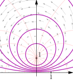
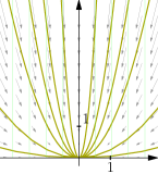
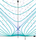
Figure 3. Actions of isotropy subgroups $K$, $N^{\prime}$ and $A^{\prime}$, which fix point $\iota$ in three EPH cases.

Figure 3 shows actions of the above isotropic subgroups on the respective numbers, we call them rotations around $\iota$. Note, that in parabolic and hyperbolic cases they fix larger sets connected with zero divisors.

It is inspiring to compare the action of subgroups $K$, $N^{\prime}$ and $A^{\prime}$ on three number systems, this is presented on Fig. 4. Some features are preserved if we move from top to bottom along the same column, that is, keep the subgroup and change the metric of the space. We also note the same system of a gradual transition if we compare pictures from left to right along a particular row. Note, that Fig. 3 extracts diagonal images from Fig. 4, this puts three images from Fig. 3 into a context, which is not obvious from Fig. 4.

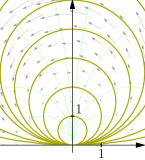
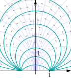
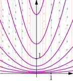
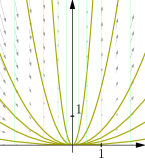
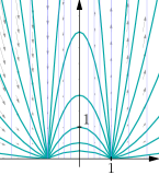
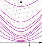
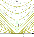
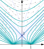
Figure 4. Actions of the subgroups $K$, $N^{\prime}$, $A^{\prime}$ are shown in the first, middle and last columns respectively. The elliptic, parabolic and hyperbolic spaces are presented in the first, middle and last rows respectively. The diagonal drawings comprise Fig. 3 and the first column Fig. 2.

2.4. The Heisenberg Group and Symplectomorphisms

Let $(s,x,y)$, where $s$, $x$, $y\in\mathbb{R}{}$, be an element of the one-dimensional Heisenberg group $\mathbb{H}{}$ [Folland89, Howe80b] also known as Weyl or Heisenberg-Weyl group. Consideration of the general case of the $n$-dimensional Heisenberg group $\mathbb{H}^{n}{}$ will be similar, but is beyond the scope of present paper. The group law on $\mathbb{H}{}$ is given as follows:

(24) $$\textstyle(s,x,y)\cdot(s^{\prime},x^{\prime},y^{\prime})=(s+s^{\prime}+\frac{1}{2}\omega(x,y;x^{\prime},y^{\prime}),x+x^{\prime},y+y^{\prime})$$

where the non-commutativity is due to $\omega$ – the symplectic form on $\mathbb{R}^{2}{}$ (4), which is the central object of the classical mechanics [Arnold91]*§ 37:

(25) $$\omega(x,y;x^{\prime},y^{\prime})=xy^{\prime}-x^{\prime}y.$$

The Heisenberg group is a non-commutative Lie group with the centre

$$Z=\{(s,0,0)\in\mathbb{H}{},\ s\in\mathbb{R}{}\}.$$

The left shifts

(26) $$\Lambda(g):f(g^{\prime})\mapsto f(g^{-1}g^{\prime})$$

act as a representation of $\mathbb{H}{}$ on a certain linear space of functions. For example, an action on $\mathcal{L}_{2}{}(\mathbb{H}{},dg)$ with respect to the Haar measure $dg=\mathrm{d}s\,\mathrm{d}x\,\mathrm{d}y$ is the left regular representation, which is unitary.

The Lie algebra $\mathfrak{h}$ of $\mathbb{H}{}$ is spanned by left-(right-)invariant vector fields

(27) $$\textstyle S^{l(r)}=\pm{\partial_{s}},\quad X^{l(r)}=\pm\partial_{x}-\frac{1}{2}y{\partial_{s}},\quad Y^{l(r)}=\pm\partial_{y}+\frac{1}{2}x{\partial_{s}}$$

on $\mathbb{H}{}$ with the Heisenberg commutator relation

(28) $$[X^{l(r)},Y^{l(r)}]=S^{l(r)}$$

and all other commutators vanishing. This is encoded in the phrase $\mathbb{H}{}$ is a nilpotent step $2$ Lie group. For simplicity, we will sometimes omit the superscript $l$ for left-invariant field.

The group of outer automorphisms of $\mathbb{H}{}$, which trivially acts on the centre of $\mathbb{H}{}$, is the symplectic group $\mathrm{Sp}(2)$ It is the group of symmetries of the symplectic form $\omega$ (25)  [Folland89]*Thm. 1.22 [Howe80a]*p. 830. The symplectic group is isomorphic to $\mathrm{SL}_{2}(\mathbb{R}{})$ considered in Sec. 2.2. The explicit action of $\mathrm{Sp}(2)$ on the Heisenberg group is:

(29) $$g:h=(s,x,y)\mapsto g(h)=(s,x^{\prime},y^{\prime})$$

where

$$g=\begin{pmatrix}a&b\\ c&d\end{pmatrix}\in\mathrm{SL}_{2}(\mathbb{R}{}),\quad\text{ and }\quad\begin{pmatrix}x^{\prime}\\ y^{\prime}\end{pmatrix}=\begin{pmatrix}a&b\\ c&d\end{pmatrix}\begin{pmatrix}x\\ y\end{pmatrix}.$$

Due to appearance of half-integer weight in the Shale–Weil representation below, we need to consider the metaplectic group $\mathrm{Mp}(2)$ which is the double cover of $\mathrm{Sp}(2)$. Then we can build the semidirect product $G=\mathbb{H}{}\rtimes\mathrm{Mp}(2)$ with the standard group law:

(30) $$(h,g)*(h^{\prime},g^{\prime})=(h*g(h^{\prime}),g*g^{\prime}),\qquad\text{where }h,h^{\prime}\in\mathbb{H}{},\quad g,g^{\prime}\in\mathrm{Mp}(2)$$

and the stars denote the respective group operations while the action $g(h^{\prime})$ is defined as the composition of the projection map $\mathrm{Mp}(2)\rightarrow{\mathrm{Sp}}(2)$ and the action (29). This group is sometimes called the Schrödinger group and it is known as the maximal kinematical invariance group of both the free Schrödinger equation and the quantum harmonic oscillator [Niederer73a]. This group is of interest not only in quantum mechanics but also in optics [ATorre10a, ATorre08a].

Consider the Lie algebra $\mathfrak{sl}_{2}$ of the group $\mathrm{SL}_{2}(\mathbb{R}{})$ (as well as groups $\mathrm{Sp}(2)$ and $\mathrm{Mp}(2)$). We again use the basis $A$, $B$, $Z$ (13) with commutators (14). Vectors $Z$, $B-Z/2$ and $B$ are generators of the one-parameter subgroups $K$, $N^{\prime}$ and $A^{\prime}$ (17), (22) and (23) respectively. Furthermore we can consider the basis $\{S,X,Y,A,B,Z\}$ of the Lie algebra $\mathfrak{g}$ of the Lie group $G=\mathbb{H}{}\rtimes\mathrm{Mp}(2)$. All non-zero commutators besides those already listed in (28) and (14) are:

(31) $$[A,X] =\textstyle\frac{1}{2}X, [B,X] =\textstyle-\frac{1}{2}Y, [Z,X] =Y;$$

(32) $$[A,Y] =\textstyle-\frac{1}{2}Y, [B,Y] =\textstyle-\frac{1}{2}X, [Z,Y] =-X.$$

3. Linear Representations and Hypercomplex Numbers

A consideration of the symmetries in analysis is natural to start from linear representations. The above geometrical actions (21) can be naturally extended to such representations by induction [Kirillov76]*§ 13.2 [Kisil97c]*§ 3.1 from a representation of a subgroup $H$. If $H$ is one-dimensional then its irreducible representation is a character, which is commonly supposed to be a complex valued. However, hypercomplex number naturally appeared in the $\mathrm{SL}_{2}(\mathbb{R}{})$ action (21), see [Kisil09c, Kisil12a], why shall we admit only $\mathrm{i}^{2}=-1$ to deliver a character then?

3.1. Hypercomplex Characters

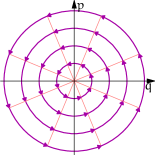
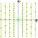
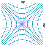
Figure 5. Rotations of algebraic wheels, i.e. the multiplication by $\mathrm{e}^{\iota t}$: elliptic ($E$), trivial parabolic ($P_{0}$) and hyperbolic ($H$). All blue orbits are defined by the identity $x^{2}-\iota^{2}y^{2}=r^{2}$. Thin “spokes” (straight lines from the origin to a point on the orbit) are “rotated” from the real axis. This is symplectic linear transformations of the classical phase space as well.

As we already mentioned, the typical discussion of induced representations of $\mathrm{SL}_{2}(\mathbb{R}{})$ is centred around the case $H=K$ and a complex valued character of $K$. A linear transformation defined by a matrix (17) in $K$ is a rotation of $\mathbb{R}^{2}{}$ by the angle $t$. After identification $\mathbb{R}^{2}{}=\mathbb{C}{}$ this action is given by the multiplication $\mathrm{e}^{\mathrm{i}t}$, with $\mathrm{i}^{2}=-1$. The rotation preserve the (elliptic) metric given by:

(33) $$x^{2}+y^{2}=(x+\mathrm{i}y)(x-\mathrm{i}y).$$

Therefore the orbits of rotations are circles, any line passing the origin (a “spoke”) is rotated by the angle $t$. Dual and double numbers produces the most straightforward adaptation of this result, see Fig. 5 for all three cases. The correspondences between the respective algebraic aspects is shown at Fig. 6.

Elliptic	Parabolic	Hyperbolic
$\mathrm{i}^{2}=-1$	$\varepsilon^{2}=0$	$\mathrm{j}^{2}=1$
$w=x+\mathrm{i}y$	$w=x+\varepsilon y$	$w=x+\mathrm{j}y$
$\bar{w}=x-\mathrm{i}y$	$\bar{w}=x-\varepsilon y$	$\bar{w}=x-\mathrm{j}y$
$\mathrm{e}^{\mathrm{i}t}=\cos t+\mathrm{i}\sin t$	$\mathrm{e}^{\varepsilon t}=1+\varepsilon t$	$\mathrm{e}^{\mathrm{j}t}=\cosh t+\mathrm{j}\sinh t$
$\left|w\right|_{e}^{2}=w\bar{w}=x^{2}+y^{2}$	$\left|w\right|_{p}^{2}=w\bar{w}=x^{2}$	$\left|w\right|_{h}^{2}=w\bar{w}=x^{2}-y^{2}$
$\arg w=\tan^{-1}\frac{y}{x}\frac{}{}$	$\arg w=\frac{y}{x}$	$\arg w=\tanh^{-1}\frac{y}{x}$
unit circle $\left|w\right|_{e}^{2}=1$	“unit” strip $x=\pm 1$	unit hyperbola $\left|w\right|_{h}^{2}=1$

Figure 6. Algebraic correspondence between complex, dual and double numbers.

Explicitly, parabolic rotations associated with $\mathrm{e}^{\varepsilon t}$ acts on dual numbers as follows:

(34) $$\mathrm{e}^{\varepsilon x}:a+\varepsilon b\mapsto a+\varepsilon(ax+b).$$

This links the parabolic case with the Galilean group [Yaglom79] of symmetries of the classic mechanics, with the absolute time disconnected from space.

The obvious algebraic similarity and the connection to classical kinematic is a wide spread justification for the following viewpoint on the parabolic case, cf. [HerranzOrtegaSantander99a, Yaglom79]:

• The parabolic trigonometric functions are trivial:

  (35) $$\mathop{\operator@font cosp}\nolimits t=\pm 1,\qquad\mathop{\operator@font sinp}\nolimits t=t.$$

• The parabolic distance is independent from $y$ if $x\neq 0$:

  (36) $$x^{2}=(x+\varepsilon y)(x-\varepsilon y).$$

• The polar decomposition of a dual number is defined by [Yaglom79]*App. C(30’):

  (37) $$u+\varepsilon v=u(1+\varepsilon\frac{v}{u}),\quad\text{ thus }\quad\left|u+\varepsilon v\right|=u,\quad\arg(u+\varepsilon v)=\frac{v}{u}.$$

• The parabolic wheel looks rectangular, see Fig. 5.

Those algebraic analogies are quite explicit and widely accepted as an ultimate source for parabolic trigonometry [LavrentShabat77, HerranzOrtegaSantander99a, Yaglom79]. Moreover, those three rotations are all non-isomorphic symplectic linear transformations of the phase space, which makes them useful in the context of classical and quantum mechanics [Kisil10a, Kisil11a], see Section 4. There exist also alternative characters [Kisil09a] based on Möbius transformations with geometric motivation and connections to equations of mathematical physics.

3.2. Induced Representations

Let $G$ be a group, $H$ be its closed subgroup with the corresponding homogeneous space $X=G/H$ with an invariant measure. Now we wish to linearise the action (18) through the induced representations [Kirillov76]*§ 13.2 [Kisil97c]*§ 3.1. We define a map $\mathsf{r}:G\rightarrow H$ associated to the natural projection $\mathsf{p}:G\rightarrow G/H$ and a continuous section $\mathsf{s}:G/H\rightarrow H$ from the identities:

(38) $$\mathsf{r}(g)={(\mathsf{s}(\omega))}^{-1}g,\qquad\text{where}\quad]\omega=\mathsf{p}(g)\in\Omega.$$

Let $\chi$ be an irreducible representation of $H$ in a vector space $V$, then it induces a representation of $G$ in the sense of Mackey [Kirillov76]*§ 13.2. For a character $\chi$ of $H$ we can define a lifting $\mathcal{L}_{\chi}:\mathcal{L}_{2}{}(G/H)\rightarrow\mathcal{L}_{2}^{\chi}{}(G)$ as follows:

(39) $$[\mathcal{L}_{\chi}f](g)=\chi(\mathbf{r}(g))f(\mathbf{p}(g))\qquad\text{where}\quad]f(x)\in\mathcal{L}_{2}{}(G/H).$$

The image space of the lifting $\mathcal{L}_{\chi}$ is invariant under left shifts. We also define the pulling $\mathcal{P}:\mathcal{L}_{2}^{\chi}{}(G)\rightarrow\mathcal{L}_{2}{}(G/H)$, which is a left inverse of the lifting and explicitly cab be given, for example, by $[\mathcal{P}F](x)=F(\mathbf{s}(x))$. Then the induced representation on $\mathcal{L}_{2}{}(G/H)$ is generated by the formula ${\rho_{\chi}}(g)=\mathcal{P}\circ\Lambda(g)\circ\mathcal{L}_{\chi}$. This representation has the realisation ${\rho_{\chi}}$ in the space of $V$-valued functions by the formula [Kirillov76]*§ 13.2.(7)–(9):

(40) $$[{\rho_{\chi}}(g)f](\omega)=\chi(\mathsf{r}(g^{-1}*\mathsf{s}(\omega)))f(g^{-1}\cdot\omega)$$

where $g\in G$, $\omega\in\Omega$, $h\in H$ and $\mathsf{r}:G\rightarrow H$, $\mathsf{s}:\Omega\rightarrow G$ are maps defined above; $*$ denotes multiplication on $G$ and $\cdot$ denotes the action (18) of $G$ on $\Omega$.

An alternative construction of induced representations is as follow [Kirillov76]*§ 13.2.

Let $\mathcal{F}_{2}^{\chi}{}(\mathbb{H}^{n}{})$ be the space of functions on $\mathbb{H}^{n}{}$ having the properties:

(41) $$f(gh)=\chi(h)f(g),\qquad\text{ for all}\quad]g\in\mathbb{H}^{n}{},\ h\in Z$$

and

(42) $$\int_{\mathbb{R}^{2n}{}}\left|f(0,x,y)\right|^{2}\,\mathrm{d}x\,\mathrm{d}y<\infty.$$

Then $\mathcal{F}_{2}^{\chi}{}(\mathbb{H}^{n}{})$ is invariant under the left shifts and those shifts restricted to $\mathcal{F}_{2}^{\chi}{}(\mathbb{H}^{n}{})$ make a representation ${\rho_{\chi}}$ of $\mathbb{H}^{n}{}$ induced by $\chi$.

Consider this scheme for representations of $\mathrm{SL}_{2}(\mathbb{R}{})$ induced from characters of its one-dimensional subgroups. We can notice that only the subgroup $K$ requires a complex valued character due to the fact of its compactness. For subgroups $N^{\prime}$ and $A^{\prime}$ we can consider characters of all three types—elliptic, parabolic and hyperbolic. Therefore we have seven essentially different induced representations. We will write explicitly only three of them here.

Example 3.1.

Consider the subgroup $H=K$, due to its compactness we are limited to complex valued characters of $K$ only. All of them are of the form $\chi_{k}$:

(43) $$\chi_{k}\begin{pmatrix}\cos t&\sin t\\ -\sin t&\cos t\end{pmatrix}=\mathrm{e}^{-\mathrm{i}kt},\qquad\text{ where}\quad]k\in\mathbb{Z}{}.$$

Using the explicit form (19) of the map $s$ we find the map $r$ given in (38) as follows:

$$r\begin{pmatrix}a&b\\ c&d\end{pmatrix}=\frac{1}{\sqrt{c^{2}+d^{2}}}\begin{pmatrix}d&-c\\ c&d\end{pmatrix}\in K.$$

Therefore:

$$\mathsf{r}(g^{-1}*\mathsf{s}(u,v))=\frac{1}{\sqrt{(cu+d)^{2}+(cv)^{2}}}\begin{pmatrix}cu+d&-cv\\ cv&cu+d\end{pmatrix}$$

where $g^{-1}=\begin{pmatrix}a&b\\ c&d\end{pmatrix}\in\mathrm{SL}_{2}(\mathbb{R}{})$. Substituting this into (43) and combining with the Möbius transformation of the domain (21) we get the explicit realisation ${\rho_{k}}{}$ of the induced representation (40):

(44) $${\rho_{k}}{}(g)f(w)=\frac{\left|cw+d\right|^{k}}{(cw+d)^{k}}f\left(\frac{aw+b}{cw+d}\right),\quad\text{ where}\quad]g^{-1}=\begin{pmatrix}a&b\\ c&d\end{pmatrix},\ w=u+\mathrm{i}v.$$

This representation acts on complex valued functions in the upper half-plane $\mathbb{R}^{2}_{+}{}=\mathrm{SL}_{2}(\mathbb{R}{})/K$ and belongs to the discrete series [Lang85]*§ IX.2. It is common to get rid of the factor $\left|cw+d\right|^{k}$ from that expression in order to keep analyticity and we will follow this practise for a convenience as well.

Example 3.2.

In the case of the subgroup $N$ there is a wider choice of possible characters.

1. Traditionally only complex valued characters of the subgroup $N$ are considered, they are:

   (45) $$\chi_{\tau}^{\mathbb{C}{}}\begin{pmatrix}1&0\\ t&1\end{pmatrix}=\mathrm{e}^{\mathrm{i}\tau t},\qquad\text{ where}\quad]\tau\in\mathbb{R}{}.$$

   A direct calculation shows that:

   $$r\begin{pmatrix}a&b\\ c&d\end{pmatrix}=\begin{pmatrix}1&0\\ \frac{c}{d}&1\end{pmatrix}\in N^{\prime}.$$

   Thus:

   (46) $$\mathsf{r}(g^{-1}*\mathsf{s}(u,v))=\begin{pmatrix}1&0\\ \frac{cv}{d+cu}&1\end{pmatrix},\quad\text{ where}\quad]g^{-1}=\begin{pmatrix}a&b\\ c&d\end{pmatrix}.$$

   A substitution of this value into the character (45) together with the Möbius transformation (21) we obtain the next realisation of (40):

   $${\rho^{\mathbb{C}{}}_{\tau}}(g)f(w)=\exp\left(\mathrm{i}\frac{\tau cv}{cu+d}\right)f\left(\frac{aw+b}{cw+d}\right)$$

   where $w=u+\varepsilon v$ and $g^{-1}=\begin{pmatrix}a&b\\ c&d\end{pmatrix}\in\mathrm{SL}_{2}(\mathbb{R}{})$. The representation acts on the space of complex valued functions on the upper half-plane $\mathbb{R}^{2}_{+}{}$, which is a subset of dual numbers as a homogeneous space $\mathrm{SL}_{2}(\mathbb{R}{})/N^{\prime}$. The mixture of complex and dual numbers in the same expression is confusing.

2. The parabolic character $\chi_{\tau}$ with the algebraic flavour is provided by multiplication (34) with the dual number:

   $$\chi_{\tau}\begin{pmatrix}1&0\\ t&1\end{pmatrix}=\mathrm{e}^{\varepsilon\tau t}=1+\varepsilon\tau t,\qquad\text{ where}\quad]\tau\in\mathbb{R}{}.$$

   If we substitute the value (46) into this character, then we receive the representation:

   $${\rho_{\tau}}{}(g)f(w)=\left(1+\varepsilon\frac{\tau cv}{cu+d}\right)f\left(\frac{aw+b}{cw+d}\right)$$

   where $w$, $\tau$ and $g$ are as above. The representation is defined on the space of dual numbers valued functions on the upper half-plane of dual numbers. Thus expression contains only dual numbers with their usual algebraic operations. Thus it is linear with respect to them.

All characters in the previous Example are unitary. Then, the general scheme [Kirillov76]*§ 13.2 implies unitarity of induced representations in suitable senses.

Theorem 3.3 ([Kisil09c]).

Both representations of $\mathrm{SL}_{2}(\mathbb{R}{})$ from Example 3.2 are unitary on the space of function on the upper half-plane $\mathbb{R}^{2}_{+}{}$ of dual numbers with the inner product:

(47) $$\left\langle f_{1},f_{2}\right\rangle=\int_{\mathbb{R}^{2}_{+}{}}f_{1}(w)\bar{f}_{2}(w)\,\frac{\mathrm{d}u\,\mathrm{d}v}{v^{2}},\qquad\text{ where}\quad]w=u+\varepsilon v$$

and we use the conjugation and multiplication of functions’ values in algebras of complex and dual numbers for representations ${\rho^{\mathbb{C}{}}_{\tau}}$ and ${\rho_{\tau}}$ respectively.

The inner product (47) is positive defined for the representation ${\rho^{\mathbb{C}{}}_{\tau}}$ but is not for the others. The respective spaces are parabolic cousins of the Krein spaces [ArovDym08], which are hyperbolic in our sense.

3.3. Similarity and Correspondence: Ladder Operators

From the above observation we can deduce the following empirical principle, which has a heuristic value.

Principle 3.4 (Similarity and correspondence).

1. Subgroups $K$, $N^{\prime}$ and $A^{\prime}$ play a similar rôle in the structure of the group $\mathrm{SL}_{2}(\mathbb{R}{})$ and its representations.

2. The subgroups shall be swapped simultaneously with the respective replacement of hypercomplex unit $\iota$.

The first part of the Principle (similarity) does not look sound alone. It is enough to mention that the subgroup $K$ is compact (and thus its spectrum is discrete) while two other subgroups are not. However, in a conjunction with the second part (correspondence) the Principle have received the following confirmations so far, see [Kisil09c] for details:

• The action of $\mathrm{SL}_{2}(\mathbb{R}{})$ on the homogeneous space $\mathrm{SL}_{2}(\mathbb{R}{})/H$ for $H=K$, $N^{\prime}$ or $A^{\prime}$ is given by linear-fractional transformations of complex, dual or double numbers respectively. Fig. 4 provides an illustration.

• Subgroups $K$, $N^{\prime}$ or $A^{\prime}$ are isomorphic to the groups of unitary rotations of respective unit cycles in complex, dual or double numbers.

• Representations induced from subgroups $K$, $N^{\prime}$ or $A^{\prime}$ are unitary if the inner product spaces of functions with values in complex, dual or double numbers.

Remark 3.5.

The principle of similarity and correspondence resembles supersymmetry between bosons and fermions in particle physics, but we have similarity between three different types of entities in our case.

3.4. Ladder Operators

We present another illustration to the Principle 3.4. Let ${\rho}$ be a representation of the group $\mathrm{SL}_{2}(\mathbb{R}{})$ in a space $V$. Consider the derived representation $\mathrm{d}{\rho}$ of the Lie algebra $\mathfrak{sl}_{2}$ [Lang85]*§ VI.1, that is:

(48) $$\mathrm{d}{\rho}(X)=\left.\frac{\mathrm{d}}{\mathrm{d}t}{\rho}(\mathrm{e}^{tX})\right|_{t=0},\qquad\text{for any }\quad X\in\mathfrak{sl}_{2}.$$

We also denote $\tilde{X}=\mathrm{d}{\rho}(X)$ for $X\in\mathfrak{sl}_{2}$. To see the structure of the representation ${\rho}$ we can decompose the space $V$ into eigenspaces of the operator $\tilde{X}$ for a suitable $X\in\mathfrak{sl}_{2}$.

3.4.1. Elliptic Ladder Operators

It would not be surprising that we are going to consider three cases: Let $X=Z$ be a generator of the subgroup $K$ (17). Since this is a compact subgroup the corresponding eigenspaces $\tilde{Z}v_{k}=\mathrm{i}kv_{k}$ are parametrised by an integer $k\in\mathbb{Z}{}$. The raising/lowering or ladder operators $L^{\!\pm}$ [Lang85]*§ VI.2 [MTaylor86]*§ 8.2 are defined by the following commutation relations:

(49) $$[\tilde{Z},L^{\!\pm}]=\lambda_{\pm}L^{\!\pm}.$$

In other words $L^{\!\pm}$ are eigenvectors for operators $\mathop{\operator@font ad}\nolimits Z$ of adjoint representation of $\mathfrak{sl}_{2}$ [Lang85]*§ VI.2.

Remark 3.6.

The existence of such ladder operators follows from the general properties of Lie algebras if the element $X\in\mathfrak{sl}_{2}$ belongs to a Cartan subalgebra. This is the case for vectors $Z$ and $B$, which are the only two non-isomorphic types of Cartan subalgebras in $\mathfrak{sl}_{2}$. However, the third case considered in this paper, the parabolic vector $B+Z/2$, does not belong to a Cartan subalgebra, yet a sort of ladder operators is still possible with dual number coefficients. Moreover, for the hyperbolic vector $B$, besides the standard ladder operators an additional pair with double number coefficients will also be described.

From the commutators (49) we deduce that $L^{\!+}v_{k}$ are eigenvectors of $\tilde{Z}$ as well:

(50) $$\tilde{Z}(L^{\!+}v_{k}) = (L^{\!+}\tilde{Z}+\lambda_{+}L^{\!+})v_{k}=L^{\!+}(\tilde{Z}v_{k})+\lambda_{+}L^{\!+}v_{k}=\mathrm{i}kL^{\!+}v_{k}+\lambda_{+}L^{\!+}v_{k}$$

$$= (\mathrm{i}k+\lambda_{+})L^{\!+}v_{k}.$$

Thus action of ladder operators on respective eigenspaces can be visualised by the diagram:

(51)

Assuming $L^{\!+}=a\tilde{A}+b\tilde{B}+c\tilde{Z}$ from the relations (14) and defining condition (49) we obtain linear equations with unknown $a$, $b$ and $c$:

$$c=0,\qquad 2a=\lambda_{+}b,\qquad-2b=\lambda_{+}a.$$

The equations have a solution if and only if $\lambda_{+}^{2}+4=0$, therefore the raising/lowering operators are

(52) $$L^{\!\pm}=\pm\mathrm{i}\tilde{A}+\tilde{B}.$$

3.4.2. Hyperbolic Ladder Operators

Consider the case $X=2B$ of a generator of the subgroup $A^{\prime}$ (23). The subgroup is not compact and eigenvalues of the operator $\tilde{B}$ can be arbitrary, however raising/lowering operators are still important [HoweTan92]*§ II.1 [Mazorchuk09a]*§ 1.1. We again seek a solution in the form $L_{h}^{\!+}=a\tilde{A}+b\tilde{B}+c\tilde{Z}$ for the commutator $[2\tilde{B},L_{h}^{\!+}]=\lambda L_{h}^{\!+}$. We will get the system:

$$4c=\lambda a,\qquad b=0,\qquad{a}=\lambda c.$$

A solution exists if and only if $\lambda^{2}=4$. There are obvious values $\lambda=\pm 2$ with the ladder operators $L_{h}^{\!\pm}=\pm 2\tilde{A}+\tilde{Z}$, see [HoweTan92]*§ II.1 [Mazorchuk09a]*§ 1.1. Each indecomposable $\mathfrak{sl}_{2}$-module is formed by a one-dimensional chain of eigenvalues with a transitive action of ladder operators.

Admitting double numbers we have an extra possibility to satisfy $\lambda^{2}=4$ with values $\lambda=\pm 2\mathrm{j}$. Then there is an additional pair of hyperbolic ladder operators $L_{\mathrm{j}}^{\!\pm}=\pm 2\mathrm{j}\tilde{A}+\tilde{Z}$, which shift eigenvectors in the “orthogonal” direction to the standard operators $L_{h}^{\!\pm}$. Therefore an indecomposable $\mathfrak{sl}_{2}$-module can be parametrised by a two-dimensional lattice of eigenvalues on the double number plane, see Fig. 7

Figure 7. The action of hyperbolic ladder operators on a 2D lattice of eigenspaces. Operators $L_{h}^{\!\pm}$ move the eigenvalues by $2$, making shifts in the horizontal direction. Operators $L_{\mathrm{j}}^{\!\pm}$ change the eigenvalues by $2\mathrm{j}$, shown as vertical shifts.

3.4.3. Parabolic Ladder Operators

Finally consider the case of a generator $X=-B+Z/2$ of the subgroup $N^{\prime}$ (22). According to the above procedure we get the equations:

$$b+2c=\lambda a,\qquad-a=\lambda b,\qquad\frac{a}{2}=\lambda c$$

which can be resolved if and only if $\lambda^{2}=0$. If we restrict ourselves with the only real (complex) root $\lambda=0$, then the corresponding operators $L_{p}^{\!\pm}=-\tilde{B}+\tilde{Z}/2$ will not affect eigenvalues and thus are useless in the above context. However the dual number roots $\lambda=\pm\varepsilon t$, $t\in\mathbb{R}{}$ lead to the operators $L_{\varepsilon}^{\!\pm}=\pm\varepsilon t\tilde{A}-\tilde{B}+\tilde{Z}/2$. These operators are suitable to build an $\mathfrak{sl}_{2}$-modules with a one-dimensional chain of eigenvalues.

Remark 3.7.

The following rôles of hypercomplex numbers are noteworthy:

• the introduction of complex numbers is a necessity for the existence of ladder operators in the elliptic case;

• in the parabolic case we need dual numbers to make ladder operators useful;

• in the hyperbolic case double numbers are not required neither for the existence or for the usability of ladder operators, but they do provide an enhancement.

We summarise the above consideration with a focus on the Principle of similarity and correspondence:

Proposition 3.8.

Let a vector $X\in\mathfrak{sl}_{2}$ generates the subgroup $K$, $N^{\prime}$ or $A^{\prime}$, that is $X=Z$, $B-Z/2$, or $B$ respectively. Let $\iota$ be the respective hypercomplex unit.

Then raising/lowering operators $L^{\!\pm}$ satisfying to the commutation relation:

$$[X,L^{\!\pm}]=\pm\iota L^{\!\pm},\qquad[L^{\!-},L^{\!+}]=2\iota X.$$

are:

$$L^{\!\pm}=\pm\iota\tilde{A}+\tilde{Y}.$$

Here $Y\in\mathfrak{sl}_{2}$ is a linear combination of $B$ and $Z$ with the properties:

• $Y=[A,X]$.

• $X=[A,Y]$.

• Killings form $K(X,Y)$ [Kirillov76]*§ 6.2 vanishes.

Any of the above properties defines the vector $Y\in\mathop{\operator@font span}\nolimits\{B,Z\}$ up to a real constant factor.

3.5. Induced Representations of the Heisenberg Group

In this subsection we calculate representations of of the Heisenberg group induced by a complex valued character. Representations induced by hypercomplex characters and their physical interpretation will be discussed in the next section.

Take a maximal (two dimensional) abelian subgroup $H=\{(s,0,y)\in\mathbb{H}{}\}$, then the homogeneous space can be parametrised by a real number $x$. We define the natural projection $\mathsf{p}(s,x,y)=x$ and the continuous section $\mathsf{s}(x)=(0,x,0)$. Then the map $\mathsf{r}:\mathbb{H}^{1}{}\rightarrow H^{\prime}_{x}$ is $\mathsf{r}(s,x,y)=(s-\frac{1}{2}xy,0,y)$. For the character $\chi_{\hslash}(s,0,y)=\mathrm{e}^{2\pi\mathrm{i}(\hslash s)}$, the representation of $\mathbb{H}^{1}{}$ on $\mathcal{L}_{2}{}(\mathbb{R}^{1}{})$ is:

(53) $$\textstyle[{\rho_{\chi}}(s,x,y)f](x^{\prime})=\exp(2\pi\mathrm{i}(\hslash(-s+yx^{\prime}-\frac{1}{2}xy)))\,f(x^{\prime}-x).$$

Then the Fourier transform $x\rightarrow q$ produces the Schrödinger representation [Folland89]*§ 1.3 of $\mathbb{H}{}$ in $\mathcal{L}_{2}{}(\mathbb{R}{})$, that is [Kisil10a]*(3.5):

(54) $$[{\rho_{\hslash}}(s,x,y)f\,](q)=\mathrm{e}^{2\pi\mathrm{i}\hslash(s-xy/2)+2\pi\mathrm{i}xq}\,f(q-\hslash y).$$

The variable $q$ is treated as the coordinate on the configurational space of a particle. The action of the derived representation on the Lie algebra $\mathfrak{h}$ is:

(55) $${\rho_{\hslash}}(X)=2\pi\mathrm{i}q,\qquad{\rho_{\hslash}}(Y)=-\hslash\frac{\mathrm{d}}{\mathrm{d}q},\qquad{\rho_{\hslash}}(S)=2\pi\mathrm{i}\hslash I.$$

The Shale–Weil theorem [Folland89]*§ 4.2 [Howe80a]*p. 830 states that any representation ${\rho_{\hslash}}$ of the Heisenberg groups generates a unitary oscillator (or metaplectic) representation ${\rho^{\text{SW}}_{\hslash}}$ of the $\mathrm{Mp}(2)$, the two-fold cover of the symplectic group [Folland89]*Thm. 4.58. The Shale–Weil theorem allows us to expand any representation ${\rho_{\hslash}}$ of the Heisenberg group to the representation ${\rho^{2}_{\hslash}}={\rho_{\hslash}}\oplus{\rho^{\text{SW}}_{\hslash}}$ of the group Schrödinger group (30). Of course, there is the derived form of the Shale–Weil representation for $\mathfrak{g}$. It can often be explicitly written in contrast to the Shale–Weil representation.

Example 3.9.

TheShale–Weil representation of $\mathrm{SL}_{2}(\mathbb{R}{})$ in $\mathcal{L}_{2}{}(\mathbb{R}{})$ associated to the Schrödinger representation (54) has the derived action, cf. [ATorre08a]*(2.2) [Folland89]*§ 4.3:

(56) $${\rho^{\text{SW}}_{\hslash}}(A)=-\frac{q}{2}\frac{\mathrm{d}}{\mathrm{d}q}-\frac{1}{4},\quad{\rho^{\text{SW}}_{\hslash}}(B)=-\frac{\hslash\mathrm{i}}{8\pi}\frac{\mathrm{d}^{2}}{\mathrm{d}q^{2}}-\frac{\pi\mathrm{i}q^{2}}{2\hslash},\quad{\rho^{\text{SW}}_{\hslash}}(Z)=\frac{\hslash\mathrm{i}}{4\pi}\frac{\mathrm{d}^{2}}{\mathrm{d}q^{2}}-\frac{\pi\mathrm{i}q^{2}}{\hslash}.$$

We can verify commutators (14) and (28), (32) for operators (55)–(56). It is also obvious that in this representation the following algebraic relations hold:

$$\qquad{\rho^{\text{SW}}_{\hslash}}(A) = \frac{\mathrm{i}}{4\pi\hslash}({\rho_{\hslash}}(X){\rho_{\hslash}}(Y)-{\textstyle\frac{1}{2}}{\rho_{\hslash}}(S))$$

$$= \frac{\mathrm{i}}{8\pi\hslash}({\rho_{\hslash}}(X){\rho_{\hslash}}(Y)+{\rho_{\hslash}}(Y){\rho_{\hslash}}(X)),$$

(58) $${\rho^{\text{SW}}_{\hslash}}(B) = \frac{\mathrm{i}}{8\pi\hslash}({\rho_{\hslash}}(X)^{2}-{\rho_{\hslash}}(Y)^{2}),$$

(59) $${\rho^{\text{SW}}_{\hslash}}(Z) = \frac{\mathrm{i}}{4\pi\hslash}({\rho_{\hslash}}(X)^{2}+{\rho_{\hslash}}(Y)^{2}).$$

Thus it is common in quantum optics to name $\mathfrak{g}$ as a Lie algebra with quadratic generators, see [Gazeau09a]*§ 2.2.4.

Note that ${\rho^{\text{SW}}_{\hslash}}(Z)$ is the Hamiltonian of the harmonic oscillator (up to a factor). Then we can consider ${\rho^{\text{SW}}_{\hslash}}(B)$ as the Hamiltonian of a repulsive (hyperbolic) oscillator. The operator ${\rho^{\text{SW}}_{\hslash}}(B-Z/2)=\frac{\hslash\mathrm{i}}{4\pi}\frac{\mathrm{d}^{2}}{\mathrm{d}q^{2}}$ is the parabolic analog. A graphical representation of all three transformations defined by those Hamiltonian is given in Fig. 5 and a further discussion of these Hamiltonians can be found in [Wulfman10a]*§ 3.8.

An important observation, which is often missed, is that the three linear symplectic transformations are unitary rotations in the corresponding hypercomplex algebra, cf. [Kisil09c]*§ 3. This means, that the symplectomorphisms generated by operators $Z$, $B-Z/2$, $B$ within time $t$ coincide with the multiplication of hypercomplex number $q+\iota p$ by $\mathrm{e}^{\iota t}$, see Subsection 3.1 and Fig. 5, which is just another illustration of the Similarity and Correspondence Principle 3.4.

Example 3.10.

There are many advantages of considering representations of the Heisenberg group on the phase space [Howe80b]*§ 1.7 [Folland89]*§ 1.6 [deGosson08a]. A convenient expression for Fock–Segal–Bargmann (FSB) representation on the phase space is, cf. § 4.2.1 and [Kisil02e]*(2.9) [deGosson08a]*(1):

(60) $$\textstyle[{\rho_{F}}(s,x,y)f](q,p)=\mathrm{e}^{-2\pi\mathrm{i}(\hslash s+qx+py)}f\left(q-\frac{\hslash}{2}y,p+\frac{\hslash}{2}x\right).$$

Then the derived representation of $\mathfrak{h}$ is:

(61) $$\textstyle{\rho_{F}}(X)=-2\pi\mathrm{i}q+\frac{\hslash}{2}\partial_{p},\qquad{\rho_{F}}(Y)=-2\pi\mathrm{i}p-\frac{\hslash}{2}\partial_{q},\qquad{\rho_{F}}(S)=-2\pi\mathrm{i}\hslash I.$$

This produces the derived form of the Shale–Weil representation:

(62) $$\textstyle{\rho^{\text{SW}}_{F}}(A)=\frac{1}{2}\left(q\partial_{q}-p\partial_{p}\right),\quad{\rho^{\text{SW}}_{F}}(B)=-\frac{1}{2}\left(p\partial_{q}+q\partial_{p}\right),\quad{\rho^{\text{SW}}_{F}}(Z)=p\partial_{q}-q\partial_{p}.$$

Note that this representation does not contain the parameter $\hslash$ unlike the equivalent representation (56). Thus, the FSB model explicitly shows the equivalence of ${\rho^{\text{SW}}_{\hslash_{1}}}$ and ${\rho^{\text{SW}}_{\hslash_{2}}}$ if $\hslash_{1}\hslash_{2}>0$ [Folland89]*Thm. 4.57.

As we will also see below the FSB-type representations in hypercomplex numbers produce almost the same Shale–Weil representations.

4. Mechanics and Hypercomplex Numbers

Complex valued representations of the Heisenberg group provide a natural framework for quantum mechanics [Howe80b, Folland89]. These representations provide the fundamental example of induced representations, the Kirillov orbit method and geometrical quantisation technique [Kirillov99, Kirillov94a]. Following the presentation in Section 3 we will consider representations of the Heisenberg group which are induced by hypercomplex characters of its centre: complex (which correspond to the elliptic case), dual (parabolic) and double (hyperbolic).

To describe dynamics of a physical system we use a universal equation based on inner derivations (commutator) of the convolution algebra [Kisil00a] [Kisil02e]. The complex valued representations produce the standard framework for quantum mechanics with the Heisenberg dynamical equation [Vourdas06a].

The double number valued representations, with the hyperbolic unit $\mathrm{j}^{2}=1$, is a natural source of hyperbolic quantum mechanics developed for a while [Hudson04a, Hudson66a, Khrennikov03a, Khrennikov05a, Khrennikov08a, Ulrych2014a]. The universal dynamical equation employs hyperbolic commutator in this case. This can be seen as a Moyal bracket based on the hyperbolic sine function. The hyperbolic observables act as operators on a Krein space with an indefinite inner product. Such spaces are employed in study of $\mathcal{PT}$-symmetric Hamiltonians and hyperbolic unit $\mathrm{j}^{2}=1$ naturally appear in this setup [GuentherKuzhel10a].

The representations with values in dual numbers provide a convenient description of the classical mechanics. For this we do not take any sort of semiclassical limit, rather the nilpotency of the parabolic unit ($\varepsilon^{2}=0$) does the task. This removes the vicious necessity to consider the Planck constant tending to zero. The dynamical equation takes the Hamiltonian form. We also describe classical non-commutative representations of the Heisenberg group which acts in the first jet space.

Remark 4.1.

It is worth to note that our technique is different from contraction technique in the theory of Lie groups [LevyLeblond65a, GromovKuratov05b, Gromov12a]. Indeed a contraction of the Heisenberg group $\mathbb{H}^{n}{}$ is the commutative Euclidean group $\mathbb{R}^{2n}{}$ which may be identified with the phase space in classical and quantum mechanics.

The considered here approach provides not only three different types of dynamics, it also generates the respective rules for addition of probabilities as well. For example, the quantum interference is the consequence of the same complex-valued structure, which directs the Heisenberg equation. The absence of an interference (a particle behaviour) in the classical mechanics is again the consequence the nilpotency of the parabolic unit. Double numbers creates the hyperbolic law of additions of probabilities, which was extensively investigates [Khrennikov03a, Khrennikov05a]. There are still unresolved issues with positivity of the probabilistic interpretation in the hyperbolic case [Hudson04a, Hudson66a].

The fundamental relations of quantum and classical mechanics were discussed in Section 1. Below we will recover the existence of three non-isomorphic models of mechanics from the representation theory. They were already derived in [Hudson04a, Hudson66a] from translation invariant formulation, that is from the group theory as well. It also hinted that hyperbolic counterpart is (at least theoretically) as natural as classical and quantum mechanics are. The approach provides a framework for a description of aggregate system which have say both quantum and classical components. This can be used to model quantum computers with classical terminals [Kisil09b].

Remarkably, simultaneously with the work [Hudson66a] group-invariant axiomatics of geometry leaded R.I. Pimenov [Pimenov65a] to description of $3^{n}$ Cayley–Klein constructions. The connection between group-invariant geometry and respective mechanics were explored in many works of N.A. Gromov, see for example [Gromov90a, Gromov90b, GromovKuratov05b]. They already highlighted the rôle of three types of hypercomplex units for the realisation of elliptic, parabolic and hyperbolic geometry and kinematic.

There is a further connection between representations of the Heisenberg group and hypercomplex numbers. The symplectomorphism of phase space are also automorphism of the Heisenberg group [Folland89]*§ 1.2. We recall that the symplectic group $\mathrm{SL}_{2}(\mathbb{R}{})$ [Folland89]*§ 1.2 is isomorphic to the group $\mathrm{SL}_{2}(\mathbb{R}{})$  [Lang85] [HoweTan92] [Mazorchuk09a] and provides linear symplectomorphisms of the two-dimensional phase space. It has three types of non-isomorphic one-dimensional continuous subgroups (15)–(17) with symplectic action on the phase space illustrated by Fig. 5. Hamiltonians, which produce those symplectomorphism, are of interest [Wulfman10a]*§ 3.8 [ATorre08a] [ATorre10a]. An analysis of those Hamiltonians from Subsection 3.3 by means of ladder operators recreates hypercomplex coefficients as well [Kisil11a].

Harmonic oscillators, which we shall use as the main illustration here, are treated in most textbooks on quantum mechanics. This is efficiently done through creation/annihilation (ladder) operators, cf. § 3.3 and [Gazeau09a] [BoyerMiller74a]. The underlying structure is the representation theory of the Heisenberg and symplectic groups [Lang85]*§ VI.2 [MTaylor86]*§ 8.2 [Howe80b] [Folland89]. As we will see, they are naturally connected with respective hypercomplex numbers. As a result we obtain further illustrations to the Similarity and Correspondence Principle 3.4.

We work with the simplest case of a particle with only one degree of freedom. Higher dimensions and the respective group of symplectomorphisms $\mathrm{Sp}(2n)$ may require consideration of Clifford algebras [Kisil93c] [ConstalesFaustinoKrausshar11a] [CnopsKisil97a] [GuentherKuzhel10a] [Porteous95] [Kisil14a] [Ulrych2014a].

4.1. p-Mechanic Formalism

Here we briefly outline a formalism [Kisil96a, Prezhdo-Kisil97, Kisil00a, BrodlieKisil03a, Kisil02e], which allows to unify quantum and classical mechanics.

4.1.1. Convolutions (Observables) on $\mathbb{H}{}$ and Commutator

Using the invariance of the Lebesgue measure $dg=\mathrm{d}s\,\mathrm{d}x\,\mathrm{d}y$ on $\mathbb{H}{}$ we can define the convolution of two functions:

(63) $$(k_{1}*k_{2})(g) = \int_{\mathbb{H}{}}k_{1}(g_{1})\,k_{2}(g_{1}^{-1}g)\,\mathrm{d}g_{1}.$$

Because $\mathbb{H}{}$ is non-commutative, the convolution is a non-commutative operation. It is meaningful for functions from various spaces including $\mathcal{L}_{1}{}(\mathbb{H}{})=\mathcal{L}_{1}{}(\mathbb{H}{},dg)$, the Schwartz space $\mathcal{S}{}$ and many classes of distributions, which form algebras under convolutions. Convolutions on $\mathbb{H}{}$ are used as observables in $p$-mechanic [Kisil96a, Kisil02e].

A unitary representation ${\rho}$ of $\mathbb{H}{}$ extends to $\mathcal{L}_{1}{}(\mathbb{H}{})$ by the formula:

(64) $${\rho}(k)=\int_{\mathbb{H}{}}k(g){\rho}(g)\,\mathrm{d}g$$

where the operator-valued integral can be defined in a weak sense. This is also an algebra homomorphism of convolutions to linear operators.

For a dynamics of observables we need inner derivations $D_{k}$ of the convolution algebra $\mathcal{L}_{1}{}(\mathbb{H}{})$, which are given by the commutator:

$$\qquad D_{k}:f\mapsto[k,f] = k*f-f*k$$

$$= \int_{\mathbb{H}{}}k(g_{1})\left(f(g_{1}^{-1}g)-f(gg_{1}^{-1})\right)\,\mathrm{d}g_{1},\quad f,k\in\mathcal{L}_{1}{}(\mathbb{H}{}).$$

To describe dynamics of a time-dependent observable $f(t,g)$ we use the universal equation, cf. [Kisil94d, Kisil96a]:

(66) $$S\dot{f}=[H,f]$$

where $S$ is the left-invariant vector field (27) generated by the centre of $\mathbb{H}{}$. The presence of operator $S$ fixes the dimensionality of both sides of the equation (66) if the observable $H$ (Hamiltonian) has the dimensionality of energy [Kisil02e]*Rem 4.1.

Alternatively, if we apply a right inverse $\mathcal{A}$ of $S$ to both sides of the equation (66) we obtain the equivalent equation

(67) $$\dot{f}=\left\{\!\left[H,f\right]\!\right\}$$

based on the universal bracket $\left\{\!\left[k_{1},k_{2}\right]\!\right\}=k_{1}*\mathcal{A}k_{2}-k_{2}*\mathcal{A}k_{1}$ [Kisil02e]. We will not use this approach in the present paper.

Example 4.2 (Harmonic oscillator).

Let $H=\frac{1}{2}(mk^{2}q^{2}+\frac{1}{m}p^{2})$ be the Hamiltonian of a one-dimensional harmonic oscillator, where $k$ is a constant frequency and $m$ is a constant mass. Its p-mechanisation will be the second order differential operator on $\mathbb{H}{}$ [BrodlieKisil03a]*§ 5.1:

$$\textstyle H=\frac{1}{2}(mk^{2}X^{2}+\frac{1}{m}Y^{2})$$

where we dropped sub-indexes of vector fields (27) in one dimensional setting. We can express the commutator as a difference between the left and the right action of the vector fields:

$$\textstyle[H,f]=\frac{1}{2}(mk^{2}((X^{r})^{2}-(X^{l})^{2})+\frac{1}{m}((Y^{r})^{2}-(Y^{l})^{2}))f.$$

Thus the equation (66) becomes [BrodlieKisil03a]*(5.2):

(68) $$\frac{\partial}{\partial s}\dot{f}=\frac{\partial}{\partial s}\left(mk^{2}y\frac{\partial}{\partial x}-\frac{1}{m}x\frac{\partial}{\partial y}\right)f.$$

Of course, the derivative $\frac{\partial}{\partial s}$ can be dropped from both sides of the equation and the general solution is found to be:

(69) $$\textstyle f(t;s,x,y)=f_{0}\left(s,x\cos(kt)+mky\sin(kt),-\frac{x}{mk}\sin(kt)+y\cos(kt)\right)$$

where $f_{0}(s,x,y)$ is the initial value of an observable on $\mathbb{H}{}$.

Example 4.3 (Unharmonic oscillator).

We consider unharmonic oscillator with cubic potential, see [CalzettaVerdaguer06a] and references therein:

(70) $$H=\frac{mk^{2}}{2}q^{2}+\frac{\lambda}{6}q^{3}+\frac{1}{2m}p^{2}.$$

Due to the absence of non-commutative products in (70), its p-mechanisation is again straightforward:

$$H=\frac{mk^{2}}{2}X^{2}+\frac{\lambda}{6}X^{3}+\frac{1}{m}Y^{2}.$$

Similarly to the harmonic case the dynamic equation, after cancellation of $\frac{\partial}{\partial s}$ on both sides, becomes:

(71) $$\dot{f}=\left(mk^{2}y\frac{\partial}{\partial x}+\frac{\lambda}{6}\left(3y\frac{\partial^{2}}{\partial x^{2}}+\frac{1}{4}y^{3}\frac{\partial^{2}}{\partial s^{2}}\right)-\frac{1}{m}x\frac{\partial}{\partial y}\right)f.$$

Unfortunately, it cannot be solved analytically as easy as in the harmonic case.

4.1.2. States and Probability

Let an observable ${\rho}(k)$ (64) is defined by a kernel $k(g)$ on the Heisenberg group and a representation ${\rho}$ at a Hilbert space $\mathcal{H}$. A state on the convolution algebra is given by a vector $v\in\mathcal{H}$. A simple calculation:

$$\left\langle{\rho}(k)v,v\right\rangle_{\mathcal{H}} = \left\langle\int_{\mathbb{H}{}}k(g){\rho}(g)v\,\mathrm{d}g,v\right\rangle_{\mathcal{H}}$$

$$= \int_{\mathbb{H}{}}k(g)\left\langle{\rho}(g)v,v\right\rangle_{\mathcal{H}}dg$$

$$= \int_{\mathbb{H}{}}k(g)\overline{\left\langle v,{\rho}(g)v\right\rangle_{\mathcal{H}}}\,\mathrm{d}g$$

can be restated as:

$$\left\langle{\rho}(k)v,v\right\rangle_{\mathcal{H}}=\left\langle k,l\right\rangle,\qquad\text{where}\quad l(g)=\left\langle v,{\rho}(g)v\right\rangle_{\mathcal{H}}.$$

Here the left-hand side contains the inner product on $\mathcal{H}$, while the right-hand side uses a skew-linear pairing between functions on $\mathbb{H}{}$ based on the Haar measure integration. In other words we obtain, cf. [BrodlieKisil03a]*Thm. 3.11:

Proposition 4.4.

A state defined by a vector $v\in\mathcal{H}$ coincides with the linear functional given by the wavelet transform

(72) $$l(g)=\left\langle v,{\rho}(g)v\right\rangle_{\mathcal{H}}$$

of $v$ used as the mother wavelet as well.

The addition of vectors in $\mathcal{H}$ implies the following operation on states:

(73) $$\left\langle v_{1}+v_{2},{\rho}(g)(v_{1}+v_{2})\right\rangle_{\mathcal{H}} = \left\langle v_{1},{\rho}(g)v_{1}\right\rangle_{\mathcal{H}}+\left\langle v_{2},{\rho}(g)v_{2}\right\rangle_{\mathcal{H}}$$

$${}+\left\langle v_{1},{\rho}(g)v_{2}\right\rangle_{\mathcal{H}}+\overline{\left\langle v_{1},{\rho}(g^{-1})v_{2}\right\rangle_{\mathcal{H}}}$$

The last expression can be conveniently rewritten for kernels of the functional as

(74) $$l_{12}=l_{1}+l_{2}+2A\sqrt{l_{1}l_{2}}$$

for some real number $A$. This formula is behind the contextual law of addition of conditional probabilities [Khrennikov01a] and will be illustrated below. Its physical interpretation is an interference, say, from two slits. Despite of a common belief, the mechanism of such interference can be both causal and local, see [Kisil01c] [KhrenVol01].

4.2. Elliptic Characters and Quantum Dynamics

In this subsection we consider the representation ${\rho_{h}}$ of the Heisenberg group $\mathbb{H}{}$ induced by the elliptic character $\chi_{h}(s)=\mathrm{e}^{\mathrm{i}hs}$ in complex numbers parametrised by $h\in\mathbb{R}{}$. We also use the convenient agreement $h=2\pi\hslash$ borrowed from physical literature.

4.2.1. Fock–Segal–Bargmann and Schrödinger Representations

The realisation of ${\rho_{h}}$ by the left shifts (26) on $\mathcal{L}_{2}^{h}{}(\mathbb{H}{})$ is rarely used in quantum mechanics. Instead two unitary equivalent forms are more common: the Schrödinger and Fock–Segal–Bargmann (FSB) representations.

The FSB representation can be obtained from the orbit method of Kirillov [Kirillov94a]. It allows spatially separate irreducible components of the left regular representation, each of them become located on the orbit of the co-adjoint representation, see [Kisil02e]*§ 2.1 [Kirillov94a] for details, we only present a brief summary here.

We identify $\mathbb{H}{}$ and its Lie algebra $\mathfrak{h}$ through the exponential map [Kirillov76]*§ 6.4. The dual $\mathfrak{h}^{*}$ of $\mathfrak{h}$ is presented by the Euclidean space $\mathbb{R}^{3}{}$ with bi-orthogonal coordinates $(\hslash,q,p)$. Then the pairing of $\mathfrak{h}^{*}$ and $\mathfrak{h}$ given by

$$\left\langle(s,x,y),(\hslash,q,p)\right\rangle=\hslash s+q\cdot x+p\cdot y.$$

This pairing can be used to defines the Fourier transform $\hat{\ }:\mathcal{L}_{2}{}(\mathbb{H}{})\rightarrow\mathcal{L}_{2}{}(\mathfrak{h}^{*})$ given by [Kirillov99]*§ 2.3:

(75) $$\hat{\phi}(F)=\int_{\mathfrak{h}^{n}}\phi(\exp X)\mathrm{e}^{-2\pi\mathrm{i}\left\langle X,F\right\rangle}\,\mathrm{d}X,\qquad\textrm{ where}\quad]X\in\mathfrak{h}^{n},\ F\in\mathfrak{h}^{*}.$$

For a fixed $\hslash$ the left regular representation (26) is mapped by the Fourier transform to the FSB type representation (60). The collection of points $(\hslash,q,p)\in\mathfrak{h}^{*}$ for a fixed $\hslash$ is naturally identified with the phase space of the system.

Remark 4.5.

It is possible to identify the case of $\hslash=0$ with classical mechanics [Kisil02e]. Indeed, a substitution of the zero value of $\hslash$ into (60) produces the commutative representation:

(76) $${\rho_{0}}(s,x,y):f(q,p)\mapsto\mathrm{e}^{-2\pi\mathrm{i}(qx+py)}f\left(q,p\right).$$

It can be decomposed into the direct integral of one-dimensional representations parametrised by the points $(q,p)$ of the phase space. The classical mechanics, including the Hamilton equation, can be recovered from those representations [Kisil02e]. However, the condition $\hslash=0$ (as well as the semiclassical limit $\hslash\rightarrow 0$) is not completely physical. Commutativity (and subsequent relative triviality) of those representation is the main reason why they are oftenly neglected. The commutativity can be outweighed by special arrangements, e.g. an antiderivative, see the discussion around (67) and [Kisil02e]*(4.1). However, the procedure is not straightforward, see discussion in [Kisil05c] [AgostiniCapraraCiccotti07a] [Kisil09a]. A direct approach using dual numbers will be shown below, cf. Rem. 4.17.

To recover the Schrödinger representation we use notations and technique of induced representations from § 3.2, see also [Kisil98a]*Ex. 4.1. The subgroup $H=\{(s,0,y)\,\mid\,s\in\mathbb{R}{},y\in\mathbb{R}^{n}{}\}\subset\mathbb{H}{}$ defines the homogeneous space $X=G/H$, which coincides with $\mathbb{R}^{n}{}$ as a manifold. The natural projection $\mathsf{p}:G\rightarrow X$ is $\mathsf{p}(s,x,y)=x$ and its left inverse $\mathsf{s}:X\rightarrow G$ can be as simple as $\mathsf{s}(x)=(0,x,0)$. For the map $\mathsf{r}:G\rightarrow H$, $\mathsf{r}(s,x,y)=(s-xy/2,0,y)$ we have the decomposition

$$(s,x,y)=\mathsf{s}(\mathsf{p}(s,x,y))*\mathsf{r}(s,x,y)=(0,x,0)*(s-\textstyle\frac{1}{2}xy,0,y).$$

For a character $\chi_{h}(s,0,y)=\mathrm{e}^{\mathrm{i}hs}$ of $H$ the lifting $\mathcal{L}_{\chi}:\mathcal{L}_{2}{}(G/H)\rightarrow\mathcal{L}_{2}^{\chi}{}(G)$ is as follows:

$$[\mathcal{L}_{\chi}f](s,x,y)=\chi_{h}(\mathsf{r}(s,x,y))\,f(\mathsf{p}(s,x,y))=\mathrm{e}^{\mathrm{i}h(s-xy/2)}f(x).$$

Thus the representation ${\rho_{\chi}}(g)=\mathcal{P}\circ\Lambda(g)\circ\mathcal{L}$ becomes:

(77) $$[{\rho_{\chi}}(s^{\prime},x^{\prime},y^{\prime})f](x)=\mathrm{e}^{-2\pi\mathrm{i}\hslash(s^{\prime}+xy^{\prime}-x^{\prime}y^{\prime}/2)}\,f(x-x^{\prime}).$$

After the Fourier transform $x\mapsto q$ (similar to one in (75)) we get the Schrödinger representation on the configuration space:

(78) $$[{\rho_{\chi}}(s^{\prime},x^{\prime},y^{\prime})\hat{f}\,](q)=\mathrm{e}^{-2\pi\mathrm{i}\hslash(s^{\prime}+x^{\prime}y^{\prime}/2)-2\pi\mathrm{i}x^{\prime}q}\,\hat{f}(q+\hslash y^{\prime}).$$

Note that this again turns into a commutative representation (multiplication by an unimodular function) if $\hslash=0$. To get the full set of commutative representations in this way we need to use the character $\chi_{(h,p)}(s,0,y)=\mathrm{e}^{2\pi\mathrm{i}(\hslash+py)}$ in the above consideration.

4.2.2. Commutator and the Heisenberg Equation

The property (41) of $\mathcal{F}_{2}^{\chi}{}(\mathbb{H}{})$ implies that the restrictions of two operators ${\rho_{\chi}}(k_{1})$ and ${\rho_{\chi}}(k_{2})$ to this space are equal if

$$\int_{\mathbb{R}{}}k_{1}(s,x,y)\,\chi(s)\,ds=\int_{\mathbb{R}{}}k_{2}(s,x,y)\,\chi(s)\,\mathrm{d}s.$$

In other words, for a character $\chi(s)=\mathrm{e}^{2\pi\mathrm{i}\hslash s}$ the operator ${\rho_{\chi}}(k)$ depends only on

$$\hat{k}_{s}(\hslash,x,y)=\int_{\mathbb{R}{}}k(s,x,y)\,\mathrm{e}^{-2\pi\mathrm{i}\hslash s}\,\mathrm{d}s$$

which is the partial Fourier transform $s\mapsto\hslash$ of $k(s,x,y)$. The restriction to $\mathcal{F}_{2}^{\chi}{}(\mathbb{H}{})$ of the composition formula for convolutions is [Kisil02e]*(3.5):

(79) $$(k^{\prime}*k)\hat{{}_{s}}=\int_{\mathbb{R}^{2n}{}}\mathrm{e}^{{\mathrm{i}h}{}(xy^{\prime}-yx^{\prime})/2}\,\hat{k}^{\prime}_{s}(\hslash,x^{\prime},y^{\prime})\,\hat{k}_{s}(\hslash,x-x^{\prime},y-y^{\prime})\,\mathrm{d}x^{\prime}\mathrm{d}y^{\prime}.$$

Under the Schrödinger representation (78) the convolution (79) defines a rule for composition of two pseudo-differential operators (PDO) in the Weyl calculus [Howe80b] [Folland89]*§ 2.3.

Consequently the representation (64) of commutator (4.1.1) depends only on its partial Fourier transform [Kisil02e]*(3.6):

$$[k^{\prime},k]\hat{{}_{s}} = 2\mathrm{i}\int_{\mathbb{R}^{2n}{}}\!\!\sin(\textstyle\frac{h}{2}(xy^{\prime}-yx^{\prime}))\,$$

$$\qquad\times\hat{k}^{\prime}_{s}(\hslash,x^{\prime},y^{\prime})\,\hat{k}_{s}(\hslash,x-x^{\prime},y-y^{\prime})\,\mathrm{d}x^{\prime}\mathrm{d}y^{\prime}.$$

Under the Fourier transform (75) this commutator is exactly the Moyal bracket [Zachos02a] for of $\hat{k}^{\prime}$ and $\hat{k}$ on the phase space.

For observables in the space $\mathcal{F}_{2}^{\chi}{}(\mathbb{H}{})$ the action of $S$ is reduced to multiplication, e.g. for $\chi(s)=\mathrm{e}^{\mathrm{i}hs}$ the action of $S$ is multiplication by $\mathrm{i}h$. Thus the equation (66) reduced to the space $\mathcal{F}_{2}^{\chi}{}(\mathbb{H}{})$ becomes the Heisenberg type equation [Kisil02e]*(4.4):

(81) $$\dot{f}=\frac{1}{\mathrm{i}h}[H,f]\hat{{}_{s}}$$

based on the above bracket (4.2.2). The Schrödinger representation (78) transforms this equation to the original Heisenberg equation.

Example 4.6.

1. Under the Fourier transform $(x,y)\mapsto(q,p)$ the p-dynamic equation (68) of the harmonic oscillator becomes:

   (82) $$\dot{f}=\left(mk^{2}q\frac{\partial}{\partial p}-\frac{1}{m}p\frac{\partial}{\partial q}\right)f.$$

   The same transform creates its solution out of (69).

2. Since $\frac{\partial}{\partial s}$ acts on $\mathcal{F}_{2}^{\chi}{}(\mathbb{H}{})$ as multiplication by $\mathrm{i}\hslash$, the quantum representation of unharmonic dynamics equation (71) is:

   (83) $$\dot{f}=\left(mk^{2}q\frac{\partial}{\partial p}+\frac{\lambda}{6}\left(3q^{2}\frac{\partial}{\partial p}-\frac{\hslash^{2}}{4}\frac{\partial^{3}}{\partial p^{3}}\right)-\frac{1}{m}p\frac{\partial}{\partial q}\right)f.$$

   This is exactly the equation for the Wigner function obtained in [CalzettaVerdaguer06a]*(30).

4.2.3. Quantum Probabilities

For the elliptic character $\chi_{h}(s)=\mathrm{e}^{\mathrm{i}hs}$ we can use the Cauchy–Schwartz inequality to demonstrate that the real number $A$ in the identity (74) is between $-1$ and $1$. Thus, we can put $A=\cos\alpha$ for some angle (phase) $\alpha$ to get the formula for counting quantum probabilities, cf. [Khrennikov03a]*(2):

(84) $$l_{12}=l_{1}+l_{2}+2\cos\alpha\,\sqrt{l_{1}l_{2}}$$

Remark 4.7.

It is interesting to note that the both trigonometric functions are employed in quantum mechanics: sine is in the heart of the Moyal bracket (4.2.2) and cosine is responsible for the addition of probabilities (84). In the essence the commutator and probabilities took respectively the odd and even parts of the elliptic character $\mathrm{e}^{\mathrm{i}hs}$.

Example 4.8.

Take a vector $v_{(a,b)}\in\mathcal{L}_{2}^{h}{}(\mathbb{H}{})$ defined by a Gaussian with mean value $(a,b)$ in the phase space for a harmonic oscillator of the mass $m$ and the frequency $k$:

(85) $$v_{(a,b)}(q,p)=\exp\left(-\frac{2\pi km}{\hslash}(q-a)^{2}-\frac{2\pi}{\hslash km}(p-b)^{2}\right).$$

A direct calculation shows:

$$\left\langle v_{(a,b)},{\rho_{\hslash}}(s,x,y)v_{(a^{\prime},b^{\prime})}\right\rangle=\frac{4}{\hslash}\exp\left(\pi\mathrm{i}\left(2s\hslash+x(a+a^{\prime})+y(b+b^{\prime})\right)\frac{}{}\right.$$

$$\left.{}-\frac{\pi}{2\hslash km}((\hslash x+b-b^{\prime})^{2}+(b-b^{\prime})^{2})-\frac{\pi km}{2\hslash}((\hslash y+a^{\prime}-a)^{2}+(a^{\prime}-a)^{2})\right)$$

$$= \frac{4}{\hslash}\exp\left(\pi\mathrm{i}\left(2s\hslash+x(a+a^{\prime})+y(b+b^{\prime})\right)\frac{}{}\right.$$

$$\left.{}-\frac{\pi}{\hslash km}((b-b^{\prime}+{\textstyle\frac{\hslash x}{2}})^{2}+({\textstyle\frac{\hslash x}{2}})^{2})-\frac{\pi km}{\hslash}((a-a^{\prime}-{\textstyle\frac{\hslash y}{2}})^{2}+({\textstyle\frac{\hslash y}{2}})^{2})\right).$$

Thus, the kernel $l_{(a,b)}=\left\langle v_{(a,b)},{\rho_{\hslash}}(s,x,y)v_{(a,b)}\right\rangle$ (72) for a state $v_{(a,b)}$ is:

(86) $$l_{(a,b)} = \frac{4}{\hslash}\exp\left(2\pi\mathrm{i}(s\hslash+xa+yb)\frac{}{}-\frac{\pi\hslash}{2km}x^{2}-\frac{\pi km\hslash}{2\hslash}y^{2}\right)$$

An observable registering a particle at a point $q=c$ of the configuration space is $\delta(q-c)$. On the Heisenberg group this observable is given by the kernel:

(87) $$X_{c}(s,x,y)=\mathrm{e}^{2\pi\mathrm{i}(s\hslash+xc)}\delta(y).$$

The measurement of $X_{c}$ on the state (85) (through the kernel (86)) predictably is:

$$\left\langle X_{c},l_{(a,b)}\right\rangle=\sqrt{\frac{2km}{\hslash}}\exp\left(-\frac{2\pi km}{\hslash}(c-a)^{2}\right).$$

Example 4.9.

Now take two states $v_{(0,b)}$ and $v_{(0,-b)}$, where for the simplicity we assume the mean values of coordinates vanish in the both cases. Then the corresponding kernel (73) has the interference terms:

$$l_{i} = \left\langle v_{(0,b)},{\rho_{\hslash}}(s,x,y)v_{(0,-b)}\right\rangle$$

$$= \frac{4}{\hslash}\exp\left(2\pi\mathrm{i}s\hslash-\frac{\pi}{2\hslash km}((\hslash x+2b)^{2}+4b^{2})-\frac{\pi\hslash km}{2}y^{2}\right).$$

The measurement of $X_{c}$ (87) on this term contains the oscillating part:

$$\left\langle X_{c},l_{i}\right\rangle=\sqrt{\frac{2km}{\hslash}}\exp\left(-\frac{2\pi km}{\hslash}c^{2}-\frac{2\pi}{km\hslash}b^{2}+\frac{4\pi\mathrm{i}}{\hslash}cb\right)$$

Therefore on the kernel $l$ corresponding to the state $v_{(0,b)}+v_{(0,-b)}$ the measurement is

$$\left\langle X_{c},l\right\rangle = 2\sqrt{\frac{2km}{\hslash}}\exp\left(-\frac{2\pi km}{\hslash}c^{2}\right)\left(1+\exp\left(-\frac{2\pi}{km\hslash}b^{2}\right)\cos\left(\frac{4\pi}{\hslash}cb\right)\right).$$

The presence of the cosine term in the last expression can generate an interference picture. In practise, it does not happen for the minimal uncertainty state (85) which we are using here: it rapidly vanishes outside of the neighbourhood of zero, where oscillations of the cosine occurs, see Fig. 8(a).

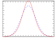
(a) (b)

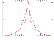
Figure 8. Quantum probabilities: the blue (dashed) graph shows the addition of probabilities without interaction, the red (solid) graph present the quantum interference. Left picture shows the Gaussian state (85), the right – the rational state (88)

Example 4.10.

To see a traditional interference pattern one can use a state which is far from the minimal uncertainty. For example, we can consider the state:

(88) $$u_{(a,b)}(q,p)=\frac{\hslash^{2}}{((q-a)^{2}+\hslash/km)((p-b)^{2}+\hslash km)}.$$

To evaluate the observable $X_{c}$ (87) on the state $l(g)=\left\langle u_{1},{\rho_{h}}(g)u_{2}\right\rangle$ (72) we use the following formula:

$$\left\langle X_{c},l\right\rangle=\frac{2}{\hslash}\int_{\mathbb{R}^{n}{}}\hat{u}_{1}(q,2(q-c)/\hslash)\,\overline{\hat{u}_{2}(q,2(q-c)/\hslash)}\,\mathrm{d}q$$

where $\hat{u}_{i}(q,x)$ denotes the partial Fourier transform $p\mapsto x$ of $u_{i}(q,p)$. The formula is obtained by swapping order of integrations. The numerical evaluation of the state obtained by the addition $u_{(0,b)}+u_{(0,-b)}$ is plotted on Fig. 8(b), the red curve shows the canonical interference pattern.

4.3. Ladder Operators and Harmonic Oscillator

Let ${\rho}$ be a representation of the Schrödinger group $G=\mathbb{H}{}\rtimes\mathrm{Mp}(2)$ (30) in a space $V$. Consider the derived representation of the Lie algebra $\mathfrak{g}$ [Lang85]*§ VI.1 and to simplify expressions we denote $\tilde{X}={\rho}(X)$ for $X\in\mathfrak{g}$. To see the structure of the representation ${\rho}$ we can decompose the space $V$ into eigenspaces of the operator $\tilde{X}$ for some $X\in\mathfrak{g}$. The canonical example is the Taylor series in complex analysis.

We are going to consider three cases corresponding to three non-isomorphic subgroups (15–17) of $\mathrm{SL}_{2}(\mathbb{R}{})$ starting from the compact case. Let $X=Z$ be a generator of the compact subgroup $K$. Corresponding symplectomorphisms (29) of the phase space are given by orthogonal rotations with matrices $\begin{pmatrix}\cos t&\sin t\\ -\sin t&\cos t\end{pmatrix}$. The Shale–Weil representation (56) coincides with the Hamiltonian of the harmonic oscillator in Schrödinger representation.

Since $\mathrm{Mp}(2)$ is a two-fold cover of $\mathrm{Mp}(2)$, the corresponding eigenspaces of a compact group $\tilde{Z}v_{k}=\mathrm{i}kv_{k}$ are parametrised by a half-integer $k\in\mathbb{Z}{}/2$. Explicitly for a half-integer $k$ eigenvectors are:

(89) $$v_{k}(q)=H_{k+\frac{1}{2}}\left(\sqrt{\frac{2\pi}{\hslash}}q\right)\mathrm{e}^{-\frac{\pi}{\hslash}q^{2}}$$

where $H_{k}$ is the Hermite polynomial [Folland89]*§ 1.7 [ErdelyiMagnusII]*8.2(9).

From the point of view of quantum mechanics as well as the representation theory, it is beneficial to introduce the ladder operators $L^{\!\pm}$ (49), known also as creation/annihilation in quantum mechanics [Folland89]*p. 49 [BoyerMiller74a]. There are two ways to search for ladder operators: in (complexified) Lie algebras $\mathfrak{h}$ and $\mathfrak{sl}_{2}$. The later coincides with our consideration in Section 3.3 in the essence.

4.3.1. Ladder Operators from the Heisenberg Group

Assuming $L^{\!+}=a\tilde{X}+b\tilde{Y}$ we obtain from the relations (31)–(32) and (49) the linear equations with unknown $a$ and $b$:

$$a=\lambda_{+}b,\qquad-b=\lambda_{+}a.$$

The equations have a solution if and only if $\lambda_{+}^{2}+1=0$, and the raising/lowering operators are $L^{\!\pm}=\tilde{X}\mp\mathrm{i}\tilde{Y}$.

Remark 4.11.

Here we have an interesting asymmetric response: due to the structure of the semidirect product $\mathbb{H}{}\rtimes\mathrm{Mp}(2)$ it is the symplectic group which acts on $\mathbb{H}{}$, not vise versa. However the Heisenberg group has a weak action in the opposite direction: it shifts eigenfunctions of $\mathrm{SL}_{2}(\mathbb{R}{})$.

In the Schrödinger representation (55) the ladder operators are

(90) $${\rho_{\hslash}}(L^{\!\pm})=2\pi\mathrm{i}q\pm\mathrm{i}\hslash\frac{\mathrm{d}}{\mathrm{d}q}.$$

The standard treatment of the harmonic oscillator in quantum mechanics, which can be found in many textbooks, e.g.  [Folland89]*§ 1.7 [Gazeau09a]*§ 2.2.3, is as follows. The vector $v_{-1/2}(q)=\mathrm{e}^{-\pi q^{2}/\hslash}$ is an eigenvector of $\tilde{Z}$ with the eigenvalue $-\frac{\mathrm{i}}{2}$. In addition $v_{-1/2}$ is annihilated by $L^{\!+}$. Thus the chain (51) terminates to the right and the complete set of eigenvectors of the harmonic oscillator Hamiltonian is presented by $(L^{\!-})^{k}v_{-1/2}$ with $k=0,1,2,\ldots$.

We can make a wavelet transform generated by the Heisenberg group with the mother wavelet $v_{-1/2}$, and the image will be the Fock–Segal–Bargmann (FSB) space [Howe80b] [Folland89]*§ 1.6. Since $v_{-1/2}$ is the null solution of $L^{\!+}=\tilde{X}-\mathrm{i}\tilde{Y}$, then by Cor. 5.3 the image of the wavelet transform will be null-solutions of the corresponding linear combination of the Lie derivatives (27):

(91) $$D=\overline{X^{r}-\mathrm{i}Y^{r}}=(\partial_{x}+\mathrm{i}\partial_{y})-\pi\hslash(x-\mathrm{i}y)$$

which turns out to be the Cauchy–Riemann equation on a weighted FSB-type space.

4.3.2. Symplectic Ladder Operators

We can also look for ladder operators within the Lie algebra $\mathfrak{sl}_{2}$, see § 3.4.1 and [Kisil09c]*§ 8. Assuming $L_{2}^{\!+}=a\tilde{A}+b\tilde{B}+c\tilde{Z}$ from the relations (14) and defining condition (49) we obtain the linear equations with unknown $a$, $b$ and $c$:

$$c=0,\qquad 2a=\lambda_{+}b,\qquad-2b=\lambda_{+}a.$$

The equations have a solution if and only if $\lambda_{+}^{2}+4=0$, and the raising/lowering operators are $L_{2}^{\!\pm}=\pm\mathrm{i}\tilde{A}+\tilde{B}$. In the Shale–Weil representation (56) they turn out to be:

(92) $$L_{2}^{\!\pm}=\pm\mathrm{i}\left(\frac{q}{2}\frac{\mathrm{d}}{\mathrm{d}q}+\frac{1}{4}\right)-\frac{\hslash\mathrm{i}}{8\pi}\frac{\mathrm{d}^{2}}{\mathrm{d}q^{2}}-\frac{\pi\mathrm{i}q^{2}}{2\hslash}=-\frac{\mathrm{i}}{8\pi\hslash}\left(\mp 2\pi q+\hslash\frac{\mathrm{d}}{\mathrm{d}q}\right)^{2}.$$

Since this time $\lambda_{+}=2\mathrm{i}$ the ladder operators $L_{2}^{\!\pm}$ produce a shift on the diagram (51) twice bigger than the operators $L^{\!\pm}$ from the Heisenberg group. After all, this is not surprising since from the explicit representations (90) and (92) we get:

$$L_{2}^{\!\pm}=-\frac{\mathrm{i}}{8\pi\hslash}(L^{\!\pm})^{2}.$$

4.4. Hyperbolic Quantum Mechanics

Now we turn to double numbers also known as hyperbolic, split-complex, etc. numbers [Yaglom79]*App. C [Ulrych05a] [KhrennikovSegre07a]. They form a two commutative associative dimensional algebra $\mathbb{O}{}$ spanned by $1$ and the hyperbolic unit $\mathrm{j}$ with the property $\mathrm{j}^{2}=1$. There are zero divisors in $\mathbb{O}{}$:

$$\mathrm{j}_{\pm}=\textstyle\frac{1}{\sqrt{2}}(1\pm j),\qquad\text{ such that }\quad\mathrm{j}_{+}\mathrm{j}_{-}=0\quad\text{ and }\quad\mathrm{j}_{\pm}^{2}=\mathrm{j}_{\pm}.$$

Thus, double numbers algebraically isomorphic to two copies of $\mathbb{R}{}$ spanned by $\mathrm{j}_{\pm}$. Being algebraically dull double numbers are nevertheless interesting as a $\mathrm{SL}_{2}(\mathbb{R}{})$-homogeneous space [Kisil05a, Kisil09c] and they are relevant in physics [Khrennikov05a, Ulrych05a, Ulrych08a, Ulrych2014a]. The combination of p-mechanical approach with hyperbolic quantum mechanics was already discussed in [BrodlieKisil03a]*§ 6.

For the hyperbolic character $\chi_{\mathrm{j}h}(s)=\mathrm{e}^{\mathrm{j}hs}=\cosh hs+\mathrm{j}\sinh hs$ of $\mathbb{R}{}$ one can define the hyperbolic Fourier-type transform:

$$\hat{k}(q)=\int_{\mathbb{R}{}}k(x)\,\mathrm{e}^{-\mathrm{j}qx}dx.$$

It can be understood in the sense of distributions on the space dual to the set of analytic functions [Khrennikov08a]*§ 3. Hyperbolic Fourier transform intertwines the derivative $\frac{\mathrm{d}}{\mathrm{d}x}$ and multiplication by $\mathrm{j}q$ [Khrennikov08a]*Prop. 1.

Example 4.12.

For the Gaussian the hyperbolic Fourier transform is the ordinary function (note the sign difference!):

$$\int_{\mathbb{R}{}}\mathrm{e}^{-x^{2}/2}\mathrm{e}^{-\mathrm{j}qx}dx=\sqrt{2\pi}\,\mathrm{e}^{q^{2}/2}.$$

However the opposite identity:

$$\int_{\mathbb{R}{}}\mathrm{e}^{x^{2}/2}\mathrm{e}^{-\mathrm{j}qx}dx=\sqrt{2\pi}\,\mathrm{e}^{-q^{2}/2}$$

is true only in a suitable distributional sense. To this end we may note that $\mathrm{e}^{x^{2}/2}$ and $\mathrm{e}^{-q^{2}/2}$ are null solutions to the differential operators $\frac{\mathrm{d}}{\mathrm{d}x}-x$ and $\frac{\mathrm{d}}{\mathrm{d}q}+q$ respectively, which are intertwined (up to the factor $\mathrm{j}$) by the hyperbolic Fourier transform. The above differential operators $\frac{\mathrm{d}}{\mathrm{d}x}-x$ and $\frac{\mathrm{d}}{\mathrm{d}q}+q$ are images of the ladder operators (90) in the Lie algebra of the Heisenberg group. They are intertwining by the Fourier transform, since this is an automorphism of the Heisenberg group [Howe80a].

An elegant theory of hyperbolic Fourier transform may be achieved by a suitable adaptation of [Howe80a], which uses representation theory of the Heisenberg group.

4.4.1. Hyperbolic Representations of the Heisenberg Group

Consider the space $\mathcal{F}_{h}^{\mathrm{j}}{}(\mathbb{H}{})$ of $\mathbb{O}{}$-valued functions on $\mathbb{H}{}$ with the property:

(93) $$f(s+s^{\prime},h,y)=\mathrm{e}^{\mathrm{j}hs^{\prime}}f(s,x,y),\qquad\text{ for all}\quad](s,x,y)\in\mathbb{H}{},\ s^{\prime}\in\mathbb{R}{}$$

and the square integrability condition (42). Then the hyperbolic representation of $\mathbb{H}{}$ is obtained by the restriction of the left shifts to $\mathcal{F}_{h}^{\mathrm{j}}{}(\mathbb{H}{})$. To obtain an equivalent representation on the phase space we take the $\mathbb{O}{}$-valued functional of the Lie algebra $\mathfrak{h}$:

(94) $$\chi^{j}_{(h,q,p)}(s,x,y)=\mathrm{e}^{\mathrm{j}(hs+qx+py)}=\cosh(hs+qx+py)+\mathrm{j}\sinh(hs+qx+py).$$

The hyperbolic Fock–Segal–Bargmann type representation is intertwined with the left group action by means of the Fourier transform (75) with the hyperbolic functional (94). Explicitly this representation is:

(95) $${\rho_{\hslash}}(s,x,y):f(q,p)\mapsto\textstyle\mathrm{e}^{-\mathrm{j}(hs+qx+py)}f\left(q-\frac{h}{2}y,p+\frac{h}{2}x\right).$$

For a hyperbolic Schrödinger type representation we again use the scheme described in § 3.2. Similarly to the elliptic case one obtains the formula, resembling (77):

(96) $$[{\rho^{\mathrm{j}}_{\chi}}(s^{\prime},x^{\prime},y^{\prime})f](x)=\mathrm{e}^{-\mathrm{j}h(s^{\prime}+xy^{\prime}-x^{\prime}y^{\prime}/2)}f(x-x^{\prime}).$$

Application of the hyperbolic Fourier transform produces a Schrödinger type representation on the configuration space, cf. (78):

$$[{\rho^{\mathrm{j}}_{\chi}}(s^{\prime},x^{\prime},y^{\prime})\hat{f}\,](q)=\mathrm{e}^{-\mathrm{j}h(s^{\prime}+x^{\prime}y^{\prime}/2)-\mathrm{j}x^{\prime}q}\,\hat{f}(q+hy^{\prime}).$$

The extension of this representation to kernels according to (64) generates hyperbolic pseudodifferential operators introduced in [Khrennikov08a]*(3.4).

4.4.2. Hyperbolic Dynamics

Similarly to the elliptic (quantum) case we consider a convolution of two kernels on $\mathbb{H}{}$ restricted to $\mathcal{F}_{h}^{\mathrm{j}}{}(\mathbb{H}{})$. The composition law becomes, cf. (79):

(97) $$(k^{\prime}*k)\hat{{}_{s}}=\int_{\mathbb{R}^{2n}{}}\mathrm{e}^{{\mathrm{j}h}{}(xy^{\prime}-yx^{\prime})}\,\hat{k}^{\prime}_{s}(h,x^{\prime},y^{\prime})\,\hat{k}_{s}(h,x-x^{\prime},y-y^{\prime})\,\mathrm{d}x^{\prime}\mathrm{d}y^{\prime}.$$

This is close to the calculus of hyperbolic PDO obtained in [Khrennikov08a]*Thm. 2. Respectively for the commutator of two convolutions we get, cf. (4.2.2):

(98) $$[k^{\prime},k]\hat{{}_{s}}=\int_{\mathbb{R}^{2n}{}}\!\!\sinh(h(xy^{\prime}-yx^{\prime}))\,\hat{k}^{\prime}_{s}(h,x^{\prime},y^{\prime})\,\hat{k}_{s}(h,x-x^{\prime},y-y^{\prime})\,\mathrm{d}x^{\prime}\mathrm{d}y^{\prime}.$$

This is the hyperbolic version of the Moyal bracket, cf. [Khrennikov08a]*p. 849, which generates the corresponding image of the dynamic equation (66).

Example 4.13.

1. For a quadratic Hamiltonian, e.g. harmonic oscillator from Example 4.2, the hyperbolic equation and respective dynamics is identical to quantum considered before.

2. Since $\frac{\partial}{\partial s}$ acts on $\mathcal{F}_{2}^{\mathrm{j}}{}(\mathbb{H}{})$ as multiplication by $\mathrm{j}h$ and $\mathrm{j}^{2}=1$, the hyperbolic image of the unharmonic equation (71) becomes:

   $$\dot{f}=\left(mk^{2}q\frac{\partial}{\partial p}+\frac{\lambda}{6}\left(3q^{2}\frac{\partial}{\partial p}+\frac{\hslash^{2}}{4}\frac{\partial^{3}}{\partial p^{3}}\right)-\frac{1}{m}p\frac{\partial}{\partial q}\right)f.$$

   The difference with quantum mechanical equation (83) is in the sign of the cubic derivative.

Notably, the hyperbolic setup allows us to linearise many non-linear problems of classical mechanics. It will be interesting to realise new hyperbolic coordinates introduced to this end in [Pilipchuk10a, Pilipchuk11a, PilipchukAndrianovMarkert16a] as a hyperbolic phase space.

4.4.3. Hyperbolic Probabilities

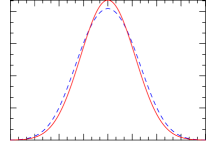
(a) (b)

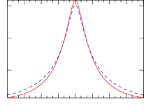
Figure 9. Hyperbolic probabilities: the blue (dashed) graph shows the addition of probabilities without interaction, the red (solid) graph present the hyperbolic quantum interference. Left picture shows the Gaussian state (85), with the same distribution as in quantum mechanics, cf. Fig. 8(a). The right picture shows the rational state (88), note the absence of interference oscillations in comparison with the quantum state on Fig. 8(b).

To calculate probability distribution generated by a hyperbolic state we are using the general procedure from Section 4.1.2. The main differences with the quantum case are as follows:

1. The real number $A$ in the expression (74) for the addition of probabilities is bigger than $1$ in absolute value. Thus, it can be associated with the hyperbolic cosine $\cosh\alpha$, cf. Rem. 4.7, for certain phase $\alpha\in\mathbb{R}{}$ [Khrennikov08a].

2. The nature of hyperbolic interference on two slits is affected by the fact that $\mathrm{e}^{\mathrm{j}hs}$ is not periodic and the hyperbolic exponent $\mathrm{e}^{\mathrm{j}t}$ and cosine $\cosh t$ do not oscillate. It is worth to notice that for Gaussian states the hyperbolic interference is exactly the same as quantum one, cf. Figs. 8(a) and 9(a). This is similar to coincidence of quantum and hyperbolic dynamics of harmonic oscillator.

   The contrast between two types of interference is prominent for the rational state (88), which is far from the minimal uncertainty, see the different patterns on Figs. 8(b) and 9(b).

4.4.4. Ladder Operators for the Hyperbolic Subgroup

Consider the case of the Hamiltonian $H=2B$, which is a repulsive (hyperbolic) harmonic oscillator [Wulfman10a]*§ 3.8. The corresponding one-dimensional subgroup of symplectomorphisms produces hyperbolic rotations of the phase space, see Fig. 5. The eigenvectors $v_{\mu}$ of the operator

$${\rho^{\text{SW}}_{\hslash}}(2B)v_{\nu}=-\mathrm{i}\left(\frac{\hslash}{4\pi}\frac{\mathrm{d}^{2}}{\mathrm{d}q^{2}}+\frac{\pi q^{2}}{\hslash}\right)v_{\nu}=\mathrm{i}\nu v_{\nu}$$

are Weber–Hermite (or parabolic cylinder) functions $v_{\nu}=D_{\nu-\frac{1}{2}}\left(\pm 2\mathrm{e}^{\mathrm{i}\frac{\pi}{4}}\sqrt{\frac{\pi}{\hslash}}q\right)$, see [ErdelyiMagnusII]*§ 8.2 [SrivastavaTuanYakubovich00a] for fundamentals of Weber–Hermite functions and [ATorre08a] for further illustrations and applications in optics.

The corresponding one-parameter group is not compact and the eigenvalues of the operator $2\tilde{B}$ are not restricted by any integrality condition, but the raising/lowering operators are still important [HoweTan92]*§ II.1 [Mazorchuk09a]*§ 1.1. We again seek solutions in two subalgebras $\mathfrak{h}$ and $\mathfrak{sl}_{2}$ separately. However, the additional options will be provided by a choice of the number system: either complex or double.

Example 4.14 (Complex Ladder Operators).

Assuming $L_{h}^{\!+}=a\tilde{X}+b\tilde{Y}$ from the commutators (31)–(32) we obtain the linear equations:

(99) $$-a=\lambda_{+}b,\qquad-b=\lambda_{+}a.$$

The equations have a solution if and only if $\lambda_{+}^{2}-1=0$. Taking the real roots $\lambda=\pm 1$ we obtain that the raising/lowering operators are $L_{h}^{\!\pm}=\tilde{X}\mp\tilde{Y}$. In the Schrödinger representation (55) the ladder operators are

(100) $$L_{h}^{\!\pm}=2\pi\mathrm{i}q\pm\hslash\frac{\mathrm{d}}{\mathrm{d}q}.$$

The null solutions $v_{\pm\frac{1}{2}}(q)=\mathrm{e}^{\pm\frac{\pi\mathrm{i}}{\hslash}q^{2}}$ to operators ${\rho_{\hslash}}(L^{\!\pm})$ are also eigenvectors of the Hamiltonian ${\rho^{\text{SW}}_{\hslash}}(2B)$ with the eigenvalue $\pm\frac{1}{2}$. However the important distinction from the elliptic case is, that they are not square-integrable on the real line anymore.

We can also look for ladder operators within the $\mathfrak{sl}_{2}$, that is in the form $L_{2h}^{\!+}=a\tilde{A}+b\tilde{B}+c\tilde{Z}$ for the commutator $[2\tilde{B},L_{h}^{\!+}]=\lambda L_{h}^{\!+}$, see § 3.4.2. Within complex numbers we get only the values $\lambda=\pm 2$ with the ladder operators $L_{2h}^{\!\pm}=\pm 2\tilde{A}+\tilde{Z}/2$, see [HoweTan92]*§ II.1 [Mazorchuk09a]*§ 1.1. Each indecomposable $\mathfrak{h}$- or $\mathfrak{sl}_{2}$-module is formed by a one-dimensional chain of eigenvalues with a transitive action of ladder operators $L_{h}^{\!\pm}$ or $L_{2h}^{\!\pm}$ respectively. And we again have a quadratic relation between the ladder operators:

$$L_{2h}^{\!\pm}=\frac{\mathrm{i}}{4\pi\hslash}(L_{h}^{\!\pm})^{2}.$$

4.4.5. Double Ladder Operators

There are extra possibilities in in the context of hyperbolic quantum mechanics [Khrennikov03a] [Khrennikov05a] [Khrennikov08a]. Here we use the representation of $\mathbb{H}{}$ induced by a hyperbolic character $\mathrm{e}^{\mathrm{j}ht}=\cosh(ht)+\mathrm{j}\sinh(ht)$, see (95) and [Kisil10a]*(4.5), and obtain the hyperbolic representation of $\mathbb{H}{}$, cf. (78):

(101) $$[{\rho^{\mathrm{j}}_{h}}(s^{\prime},x^{\prime},y^{\prime})\hat{f}\,](q)=\mathrm{e}^{\mathrm{j}h(s^{\prime}-x^{\prime}y^{\prime}/2)+\mathrm{j}x^{\prime}q}\,\hat{f}(q-hy^{\prime}).$$

The corresponding derived representation is

(102) $${\rho^{\mathrm{j}}_{h}}(X)=\mathrm{j}q,\qquad{\rho^{\mathrm{j}}_{h}}(Y)=-h\frac{\mathrm{d}}{\mathrm{d}q},\qquad{\rho^{\mathrm{j}}_{h}}(S)=\mathrm{j}hI.$$

Then the associated Shale–Weil derived representation of $\mathfrak{sp}_{2}$ in the Schwartz space $\mathcal{S}{}(\mathbb{R}{})$ is, cf. (56):

(103) $${\rho^{\text{SW}}_{h}}(A)=-\frac{q}{2}\frac{\mathrm{d}}{\mathrm{d}q}-\frac{1}{4},\quad{\rho^{\text{SW}}_{h}}(B)=\frac{\mathrm{j}h}{4}\frac{\mathrm{d}^{2}}{\mathrm{d}q^{2}}-\frac{\mathrm{j}q^{2}}{4h},\quad{\rho^{\text{SW}}_{h}}(Z)=-\frac{\mathrm{j}h}{2}\frac{\mathrm{d}^{2}}{\mathrm{d}q^{2}}-\frac{\mathrm{j}q^{2}}{2h}.$$

Note that ${\rho^{\text{SW}}_{h}}(B)$ now generates a usual harmonic oscillator, not the repulsive one like ${\rho^{\text{SW}}_{\hslash}}(B)$ in (56). However, the expressions in the quadratic algebra are still the same (up to a factor), cf. (3.9)–(59):

$$\qquad{\rho^{\text{SW}}_{h}}(A) =-\frac{\mathrm{j}}{2h}({\rho^{\mathrm{j}}_{h}}(X){\rho^{\mathrm{j}}_{h}}(Y)-{\textstyle\frac{1}{2}}{\rho^{\mathrm{j}}_{h}}(S))$$

$$=-\frac{\mathrm{j}}{4h}({\rho^{\mathrm{j}}_{h}}(X){\rho^{\mathrm{j}}_{h}}(Y)+{\rho^{\mathrm{j}}_{h}}(Y){\rho^{\mathrm{j}}_{h}}(X)),$$

$${\rho^{\text{SW}}_{h}}(B) =\frac{\mathrm{j}}{4h}({\rho^{\mathrm{j}}_{h}}(X)^{2}-{\rho^{\mathrm{j}}_{h}}(Y)^{2}),$$

$${\rho^{\text{SW}}_{h}}(Z) =-\frac{\mathrm{j}}{2h}({\rho^{\mathrm{j}}_{h}}(X)^{2}+{\rho^{\mathrm{j}}_{h}}(Y)^{2}).$$

This is due to the Principle 3.4 of similarity and correspondence: we can swap operators $Z$ and $B$ with simultaneous replacement of hypercomplex units $\mathrm{i}$ and $\mathrm{j}$.

The eigenspace of the operator $2{\rho^{\text{SW}}_{h}}(B)$ with an eigenvalue $\mathrm{j}\nu$ are spanned by the Weber–Hermite functions $D_{-\nu-\frac{1}{2}}\left(\pm\sqrt{\frac{2}{h}}x\right)$, see [ErdelyiMagnusII]*§ 8.2. Functions $D_{\nu}$ are generalisations of the Hermit functions (89).

The compatibility condition for a ladder operator within the Lie algebra $\mathfrak{h}$ will be (99) as before, since it depends only on the commutators (31)–(32). Thus, we still have the set of ladder operators corresponding to values $\lambda=\pm 1$:

$$L_{h}^{\!\pm}=\tilde{X}\mp\tilde{Y}=\mathrm{j}q\pm h\frac{\mathrm{d}}{\mathrm{d}q}.$$

Admitting double numbers we have an extra way to satisfy $\lambda^{2}=1$ in (99) with values $\lambda=\pm\mathrm{j}$. Then there is an additional pair of hyperbolic ladder operators, which are identical (up to factors) to (90):

$$L_{\mathrm{j}}^{\!\pm}=\tilde{X}\mp\mathrm{j}\tilde{Y}=\mathrm{j}q\pm\mathrm{j}h\frac{\mathrm{d}}{\mathrm{d}q}.$$

Pairs $L_{h}^{\!\pm}$ and $L_{\mathrm{j}}^{\!\pm}$ shift eigenvectors in the “orthogonal” directions changing their eigenvalues by $\pm 1$ and $\pm\mathrm{j}$. Therefore an indecomposable $\mathfrak{sl}_{2}$-module can be parametrised by a two-dimensional lattice of eigenvalues in double numbers, see Fig. 7.

The following functions

$$v_{\frac{1}{2}}^{\pm h}(q) = \mathrm{e}^{\mp\mathrm{j}q^{2}/(2h)}=\cosh\frac{q^{2}}{2h}\mp\mathrm{j}\sinh\frac{q^{2}}{2h},$$

$$v_{\frac{1}{2}}^{\pm\mathrm{j}}(q) = \mathrm{e}^{\mp q^{2}/(2h)}$$

are null solutions to the operators $L_{h}^{\!\pm}$ and $L_{\mathrm{j}}^{\!\pm}$ respectively. They are also eigenvectors of $2{\rho^{\text{SW}}_{h}}(B)$ with eigenvalues $\mp\frac{\mathrm{j}}{2}$ and $\mp\frac{1}{2}$ respectively. If these functions are used as mother wavelets for the wavelet transforms generated by the Heisenberg group, then the image space will consist of the null-solutions of the following differential operators, see Cor. 5.3:

$$\textstyle D_{h} =\overline{X^{r}-Y^{r}}=(\partial_{x}-\partial_{y})+\frac{h}{2}(x+y)$$

$$D_{\mathrm{j}} =\overline{X^{r}-\mathrm{j}Y^{r}}=(\partial_{x}+\mathrm{j}\partial_{y})-\frac{h}{2}(x-\mathrm{j}y)$$

for $v_{\frac{1}{2}}^{\pm h}$ and $v_{\frac{1}{2}}^{\pm\mathrm{j}}$ respectively. This is again in line with the classical result (91). However, annihilation of the eigenvector by a ladder operator does not mean that the part of the 2D-lattice becomes void since it can be reached via alternative routes on this lattice. Instead of multiplication by a zero, as it happens in the elliptic case, a half-plane of eigenvalues will be multiplied by the divisors of zero $1\pm\mathrm{j}$.

We can also search ladder operators within the algebra $\mathfrak{sl}_{2}$ and admitting double numbers we will again find two sets of them, cf. § 3.4.2:

$$L_{2h}^{\!\pm} = \pm\tilde{A}+\tilde{Z}/2=\mp\frac{q}{2}\frac{\mathrm{d}}{\mathrm{d}q}\mp\frac{1}{4}-\frac{\mathrm{j}h}{4}\frac{\mathrm{d}^{2}}{\mathrm{d}q^{2}}-\frac{\mathrm{j}q^{2}}{4h}=-\frac{\mathrm{j}}{4h}(L_{h}^{\!\pm})^{2},$$

$$L_{2\mathrm{j}}^{\!\pm} = \pm\mathrm{j}\tilde{A}+\tilde{Z}/2=\mp\frac{\mathrm{j}q}{2}\frac{\mathrm{d}}{\mathrm{d}q}\mp\frac{\mathrm{j}}{4}-\frac{\mathrm{j}h}{4}\frac{\mathrm{d}^{2}}{\mathrm{d}q^{2}}-\frac{\mathrm{j}q^{2}}{4h}=-\frac{\mathrm{j}}{4h}(L_{\mathrm{j}}^{\!\pm})^{2}.$$

Again the operators $L_{2h}^{\!\pm}$ and $L_{2h}^{\!\pm}$ produce double shifts in the orthogonal directions on the same two-dimensional lattice in Fig. 7.

4.5. Parabolic (Classical) Representations on the Phase Space

After the previous two cases it is natural to link classical mechanics with dual numbers generated by the parabolic unit $\varepsilon^{2}=0$. Connection of the parabolic unit $\varepsilon$ with the Galilean group of symmetries of classical mechanics is around for a while [Yaglom79]*App. C, for other applications see [CatoniCannataNichelatti04] [Zejliger34]*§ I.2(10) [Gromov90a] [Dimentberg78a] [Dimentberg78b].

However, the nilpotency of the parabolic unit $\varepsilon$ makes it difficult if we will work with dual number valued functions only. To overcome this issue we consider a commutative and associative four-dimensional real algebra $\mathfrak{C}$ spanned by $1$, $\mathrm{i}$, $\varepsilon$ and $\mathrm{i}\varepsilon$ with identities $\mathrm{i}^{2}=-1$ and $\varepsilon^{2}=0$. A seminorm on $\mathfrak{C}$ is defined as follows:

$$\left|a+b\mathrm{i}+c\varepsilon+d\mathrm{i}\varepsilon\right|^{2}=a^{2}+b^{2}.$$

4.5.1. Classical Non-Commutative Representations

We wish to build a representation of the Heisenberg group which will be a classical analog of the Fock–Segal–Bargmann representation (60). To this end, we introduce the space $\mathcal{F}_{h}^{\varepsilon}{}(\mathbb{H}{})$ of $\mathfrak{C}$-valued functions on $\mathbb{H}{}$ with the property:

(104) $$f(s+s^{\prime},h,y)=\mathrm{e}^{\varepsilon hs^{\prime}}f(s,x,y),\qquad\text{ for all}\quad](s,x,y)\in\mathbb{H}{},\ s^{\prime}\in\mathbb{R}{}$$

and the square integrability condition (42). Here as before, $\mathrm{e}^{\varepsilon hs^{\prime}}=1+\varepsilon hs^{\prime}$ in line with the Taylor expansion of the exponent. The described space is invariant under the left shifts and we restrict the left group action to $\mathcal{F}_{h}^{\varepsilon}{}(\mathbb{H}{})$.

An equivalent form of the induced representation acts on $\mathcal{F}_{h}^{\varepsilon}{}(\mathbb{R}^{2n}{})$, where $\mathbb{R}^{2n}{})$ is the homogeneous space of $\mathbb{H}{}$ over its centre. The Fourier transform $(x,y)\mapsto(q,p)$ intertwines the last representation with the following action on $\mathfrak{C}$-valued functions on the phase space:

$${\rho^{\varepsilon}_{h}}(s,x,y):f(q,p) \mapsto \mathrm{e}^{-2\pi\mathrm{i}(xq+yp)}(f(q,p)$$

$$\qquad+\varepsilon\hbar(2\pi sf(q,p)-\frac{y\mathrm{i}}{2}f^{\prime}_{q}(q,p)+\frac{x\mathrm{i}}{2}f^{\prime}_{p}(q,p))).$$

Note, that for any real polynomial $p(x)$ algebraic manipulations show that $p(x+\varepsilon y)=p(x)+\varepsilon yp^{\prime}(x)$. If extend this rule to any differentiable function then (4.5.1) can be re-written as:

(106) $${\rho_{\hslash}}(s,x,y):f(q,p)\mapsto\mathrm{e}^{-2\pi(\varepsilon\hslash s+\mathrm{i}(qx+py))}f\left(q-\frac{\mathrm{i}\hslash}{2}\varepsilon y,p+\frac{\mathrm{i}\hslash}{2}\varepsilon x\right).$$

The later form completely agrees with FSB representation (60).

Remark 4.15.

Comparing the traditional infinite-dimensional (60) and one-dimensional (76) representations of $\mathbb{H}{}$ we can note that the properties of the representation (4.5.1) are a non-trivial mixture of the former:

1. The action (4.5.1) is non-commutative, similarly to the quantum representation (60) and unlike the classical one (76). This non-commutativity will produce the Hamilton equations below in a way very similar to Heisenberg equation, see Rem. 4.17.

2. The representation (4.5.1) does not change the support of a function $f$ on the phase space, similarly to the classical representation (76) and unlike the quantum one (60). Such a localised action will be responsible later for an absence of an interference in classical probabilities.

3. The parabolic representation (4.5.1) can not be derived from either the elliptic (60) or hyperbolic (95) by the plain substitution $h=0$.

We may also write a classical Schrödinger type representation. According to § 3.2 we get a representation formally very similar to the elliptic (77) and hyperbolic versions (96):

$$[{\rho^{\varepsilon}_{\chi}}(s^{\prime},x^{\prime},y^{\prime})f](x) = \mathrm{e}^{-\varepsilon h(s^{\prime}+xy^{\prime}-x^{\prime}y^{\prime}/2)}f(x-x^{\prime})$$

$$= (1-\varepsilon h(s^{\prime}+xy^{\prime}-\textstyle\frac{1}{2}x^{\prime}y^{\prime}))f(x-x^{\prime}).$$

However due to nilpotency of $\varepsilon$ the (complex) Fourier transform $x\mapsto q$ produces a different formula for parabolic Schrödinger type representation in the configuration space, cf. (78) and (101):

$$[{\rho^{\varepsilon}_{\chi}}(s^{\prime},x^{\prime},y^{\prime})\hat{f}](q) =\mathrm{e}^{2\pi\mathrm{i}x^{\prime}q}\left(\left(1-\varepsilon h(s^{\prime}-{\textstyle\frac{1}{2}}x^{\prime}y^{\prime})\right)\hat{f}(q)+\varepsilon\mathrm{i}\hbar y^{\prime}\hat{f}^{\prime}(q)\right)$$

(108) $$=\mathrm{e}^{2\pi(-\varepsilon\hbar(s^{\prime}-{\textstyle\frac{1}{2}}x^{\prime}y^{\prime})+\mathrm{i}x^{\prime}q)}\hat{f}(q+\varepsilon\mathrm{i}\hbar y^{\prime}).$$

This representation shares all properties mentioned in Rem. 4.15 as well.

4.5.2. Hamilton Equation

The identity $\mathrm{e}^{\varepsilon t}-\mathrm{e}^{-\varepsilon t}=2\varepsilon t$ suggests that a parabolic version of the sine function is the identity function, while the parabolic cosine is identically equal to one, cf. § 3.1 and [HerranzOrtegaSantander99a, Kisil07a]. From this we obtain the parabolic version of the commutator (4.2.2):

$$[k^{\prime},k]\hat{{}_{s}}(\varepsilon h,x,y) = \varepsilon h\int_{\mathbb{R}^{2n}{}}(xy^{\prime}-yx^{\prime})$$

$${}\times\,\hat{k}^{\prime}_{s}(\varepsilon h,x^{\prime},y^{\prime})\,\hat{k}_{s}(\varepsilon h,x-x^{\prime},y-y^{\prime})\,\mathrm{d}x^{\prime}\mathrm{d}y^{\prime},$$

for the partial parabolic Fourier-type transform $\hat{k}_{s}$ of the kernels. Thus, the parabolic representation of the dynamical equation (66) becomes:

(109) $$\varepsilon h\frac{\mathrm{d}\hat{f}_{s}}{\mathrm{d}t}(\varepsilon h,x,y;t)$$

$$= \varepsilon h\int_{\mathbb{R}^{2n}{}}(xy^{\prime}-yx^{\prime})\,\hat{H}_{s}(\varepsilon h,x^{\prime},y^{\prime})\,\hat{f}_{s}(\varepsilon h,x-x^{\prime},y-y^{\prime};t)\,\mathrm{d}x^{\prime}\mathrm{d}y^{\prime}.$$

Although there is no possibility to divide by $\varepsilon$ (since it is a zero divisor) we can obviously eliminate $\varepsilon h$ from the both sides if the rest of the expressions are real. Moreover, this can be done “in advance” through a kind of the antiderivative operator considered in [Kisil02e]*(4.1). This will prevent “imaginary parts” of the remaining expressions (which contain the factor $\varepsilon$) from vanishing.

Remark 4.16.

It is noteworthy that the Planck constant completely disappeared from the dynamical equation. Thus the only prediction about it following from our construction is $h\neq 0$, which was confirmed by experiments, of course.

Using the duality between the Lie algebra $\mathfrak{h}$ of $\mathbb{H}{}$ and the phase space we can find an adjoint equation for observables on the phase space. To this end we apply the usual Fourier transform $(x,y)\mapsto(q,p)$. It turn to be the Hamilton equation (12) [Kisil02e]*(4.7). However, the transition to the phase space is more a custom rather than a necessity and in many cases we can efficiently work on the Heisenberg group itself.

Remark 4.17.

It is noteworthy, that the non-commutative representation (4.5.1) allows to obtain the Hamilton equation directly from the commutator $[{\rho^{\varepsilon}_{h}}(k_{1}),{\rho^{\varepsilon}_{h}}(k_{2})]$. Indeed, its straightforward evaluation will produce exactly the above expression. On the contrast such a commutator for the commutative representation (76) is zero and to obtain the Hamilton equation we have to work with an additional tools, e.g. an anti-derivative [Kisil02e]*(4.1).

Example 4.18.

1. For the harmonic oscillator in Example 4.2 the equation (109) again reduces to the form (68) with the solution given by (69). The adjoint equation of the harmonic oscillator on the phase space is not different from the quantum written in Example 4.6(1). This is true for any Hamiltonian of at most quadratic order.

2. For non-quadratic Hamiltonians classical and quantum dynamics are different, of course. For example, the cubic term of $\partial_{s}$ in the equation (71) will generate the factor $\varepsilon^{3}=0$ and thus vanish. Thus the equation (109) of the unharmonic oscillator on $\mathbb{H}{}$ becomes:

   $$\dot{f}=\left(mk^{2}y\frac{\partial}{\partial x}+\frac{\lambda y}{2}\frac{\partial^{2}}{\partial x^{2}}-\frac{1}{m}x\frac{\partial}{\partial y}\right)f.$$

   The adjoint equation on the phase space is:

   $$\dot{f}=\left(\left(mk^{2}q+\frac{\lambda}{2}q^{2}\right)\frac{\partial}{\partial p}-\frac{1}{m}p\frac{\partial}{\partial q}\right)f.$$

   The last equation is the classical Hamilton equation generated by the cubic potential (70). Qualitative analysis of its dynamics can be found in many textbooks [Arnold91]*§ 4.C, Pic. 12 [PercivalRichards82]*§ 4.4.

Remark 4.19.

We have obtained the Poisson bracket from the commutator of convolutions on $\mathbb{H}{}$ without any quasiclassical limit $h\rightarrow 0$. This has a common source with the deduction of main calculus theorems in [CatoniCannataNichelatti04] based on dual numbers. As explained in [Kisil05a]*Rem. 6.9 this is due to the similarity between the parabolic unit $\varepsilon$ and the infinitesimal number used in non-standard analysis [Devis77]. In other words, we never need to take care about terms of order $O(h^{2})$ because they will be wiped out by $\varepsilon^{2}=0$.

An alternative derivation of classical dynamics from the Heisenberg group is given in the recent paper [Low09a].

4.5.3. Classical Probabilities

It is worth to notice that dual numbers are not only helpful in reproducing classical Hamiltonian dynamics, they also provide the classic rule for addition of probabilities. We use the same formula (72) to calculate kernels of the states. The important difference now that the representation (4.5.1) does not change the support of functions. Thus if we calculate the correlation term $\left\langle v_{1},{\rho}(g)v_{2}\right\rangle$ in (73), then it will be zero for every two vectors $v_{1}$ and $v_{2}$ which have disjoint supports in the phase space. Thus no interference similar to quantum or hyperbolic cases (Subsection 4.2.3) is possible.

4.5.4. Ladder Operator for the Nilpotent Subgroup

Finally we look for ladder operators for the Hamiltonian $\tilde{B}+\tilde{Z}/2$ or, equivalently, $-\tilde{B}+\tilde{Z}/2$. It can be identified with a free particle [Wulfman10a]*§ 3.8.

We can search for ladder operators in the representation (55)–(56) within the Lie algebra $\mathfrak{h}$ in the form $L_{\varepsilon}^{\!\pm}=a\tilde{X}+b\tilde{Y}$. This is possible if and only if

(110) $$-b=\lambda a,\quad 0=\lambda b.$$

The compatibility condition $\lambda^{2}=0$ implies $\lambda=0$ within complex numbers. However, such a “ladder” operator $L_{\varepsilon}^{\!\pm}=a\tilde{X}$ produces only the zero shift on the eigenvectors, cf. (50).

Another possibility appears if we consider the representation of the Heisenberg group induced by dual-valued characters. On the configuration space such a representation is (108):

(111) $$[{\rho^{\varepsilon}_{\chi}}(s^{\prime},x^{\prime},y^{\prime})\hat{f}](q)=\mathrm{e}^{2\pi(-\varepsilon\hbar(s^{\prime}-{\textstyle\frac{1}{2}}x^{\prime}y^{\prime})+\mathrm{i}x^{\prime}q)}\hat{f}(q+\varepsilon\mathrm{i}\hbar y^{\prime}).$$

The corresponding derived representation of $\mathfrak{h}$ is

$${\rho^{\varepsilon}_{h}}(X)=2\pi\mathrm{i}q,\qquad{\rho^{\varepsilon}_{h}}(Y)={-\mathrm{i}\varepsilon\hbar}\frac{\mathrm{d}}{\mathrm{d}q},\qquad{\rho^{\varepsilon}_{h}}(S)=-2\pi\varepsilon\hbar I.$$

However, the Shale–Weil extension generated by this representation is inconvenient. It is better to consider the FSB–type parabolic representation (4.5.1) on the phase space induced by the same dual-valued character. Then the derived representation of $\mathfrak{h}$ is:

(112) $${\rho^{p}_{h}}(X)=-2\pi\mathrm{i}q+\frac{\mathrm{i}\varepsilon\hbar}{2}\partial_{p},\qquad{\rho^{p}_{h}}(Y)=-2\pi\mathrm{i}p-\frac{\mathrm{i}\varepsilon\hbar}{2}\partial_{q},\qquad{\rho^{p}_{h}}(S)=2\pi\varepsilon\hbar I.$$

An advantage of the FSB representation is that the derived form of the parabolic Shale–Weil representation coincides with the elliptic one (62).

Eigenfunctions with the eigenvalue $\mu$ of the parabolic Hamiltonian $\tilde{B}+\tilde{Z}/2=q\partial_{p}$ have the form

(113) $$v_{\mu}(q,p)=\mathrm{e}^{\mu p/q}f(q),\quad\text{ with an arbitrary function}\quad f(q).$$

The linear equations defining the corresponding ladder operator $L_{\varepsilon}^{\!\pm}=a\tilde{X}+b\tilde{Y}$ in the algebra $\mathfrak{h}$ are (110). The compatibility condition $\lambda^{2}=0$ implies $\lambda=0$ within complex numbers again. Admitting dual numbers we have additional values $\lambda=\pm\varepsilon\lambda_{1}$ with $\lambda_{1}\in\mathbb{C}{}$ with the corresponding ladder operators

$$L_{\varepsilon}^{\!\pm}=\tilde{X}\mp\varepsilon\lambda_{1}\tilde{Y}=-2\pi\mathrm{i}q+\frac{\mathrm{i}\varepsilon\hbar}{2}\partial_{p}\pm 2\pi\mathrm{i}\varepsilon\lambda_{1}p=-2\pi\mathrm{i}q+\varepsilon\mathrm{i}(\pm 2\pi\lambda_{1}p+\frac{\hbar}{2}\partial_{p}).$$

For the eigenvalue $\mu=\mu_{0}+\varepsilon\mu_{1}$ with $\mu_{0}$, $\mu_{1}\in\mathbb{C}{}$ the eigenfunction (113) can be rewritten as:

(114) $$v_{\mu}(q,p)=\mathrm{e}^{\mu p/q}f(q)=\mathrm{e}^{\mu_{0}p/q}\left(1+\varepsilon\mu_{1}\frac{p}{q}\right)f(q)$$

due to the nilpotency of $\varepsilon$. Then the ladder action of $L_{\varepsilon}^{\!\pm}$ is $\mu_{0}+\varepsilon\mu_{1}\mapsto\mu_{0}+\varepsilon(\mu_{1}\pm\lambda_{1})$. Therefore these operators are suitable for building $\mathfrak{sl}_{2}$-modules with a one-dimensional chain of eigenvalues.

Finally, consider the ladder operator for the same element $B+Z/2$ within the Lie algebra $\mathfrak{sl}_{2}$, cf. § 3.4.3. There is the only operator $L_{p}^{\!\pm}=\tilde{B}+\tilde{Z}/2$ corresponding to complex coefficients, which does not affect the eigenvalues. However the dual numbers lead to the operators

$$L_{\varepsilon}^{\!\pm}=\pm\varepsilon\lambda_{2}\tilde{A}+\tilde{B}+\tilde{Z}/2=\pm\frac{\varepsilon\lambda_{2}}{2}\left(q\partial_{q}-p\partial_{p}\right)+q\partial_{p},\qquad\lambda_{2}\in\mathbb{C}{}.$$

These operator act on eigenvalues in a non-trivial way.

5. Wavelet Transform, Uncertainty Relation and Analyticity

There are two and a half main examples of reproducing kernel spaces of analytic function. One is the Fock–Segal–Bargmann (FSB) space and others (one and a half) – the Bergman and Hardy spaces on the upper half-plane. The first space is generated by the Heisenberg group [Kisil11c]*§ 7.3 [Folland89]*§ 1.6, two others – by the group $\mathrm{SL}_{2}(\mathbb{R}{})$ [Kisil11c]*§ 4.2 (this explains our way of counting).

Those spaces have the following properties, which make their study particularly pleasant and fruitful:

1. There is a group, which acts transitively on functions’ domain.

2. There is a reproducing kernel.

3. The space consists of holomorphic functions.

Furthermore, for FSB space there is the following property:

1. The reproducing kernel is generated by a function, which minimises the uncertainty for coordinate and momentum observables.

It is known, that a transformation group is responsible for the appearance of the reproducing kernel [AliAntGaz00]*Thm. 8.1.3. This paper shows that the last two properties are equivalent and connected to the group as well.

5.1. Induced Wavelet (Covariant) Transform

The following object is common in quantum mechanics [Kisil02e], signal processing, harmonic analysis [Kisil12d], operator theory [Kisil12b, Kisil13a] and many other areas [Kisil11c]. Therefore, it has various names [AliAntGaz00]: coherent states, wavelets, matrix coefficients, etc. In the most fundamental situation [AliAntGaz00]*Ch. 8, we start from an irreducible unitary representation ${\rho}$ of a Lie group $G$ in a Hilbert space $\mathcal{H}{}$. For a vector $f\in\mathcal{H}{}$ (called mother wavelet, vacuum state, etc.), we define the map $\mathcal{W}_{f}$ from $\mathcal{H}{}$ to a space of functions on $G$ by:

(115) $$[\mathcal{W}_{f}v](g)=\tilde{v}(g):=\left\langle v,{\rho}(g)f\right\rangle.$$

Under the above assumptions, $\tilde{v}(g)$ is a bounded continuous function on $G$. The map $\mathcal{W}_{f}$ intertwines ${\rho}(g)$ with the left shifts on $G$:

(116) $$\mathcal{W}_{f}\circ{\rho}(g)=\Lambda(g)\circ\mathcal{W}_{f},\qquad\text{ where}\quad]\Lambda(g):\tilde{v}(g^{\prime})\mapsto\tilde{v}(g^{-1}g^{\prime}).$$

Thus, the image $\mathcal{W}_{f}\mathcal{H}{}$ is invariant under the left shifts on $G$. If ${\rho}$ is square integrable and $f$ is admissible [AliAntGaz00]*§ 8.1, then $\tilde{v}(g)$ is square-integrable with respect to the Haar measure on $G$. Moreover, it is a reproducing kernel Hilbert space and the kernel is $k(g)=[\mathcal{W}_{f}f](g)$. At this point, none of admissible vectors has an advantage over others.

It is common [Kisil11c]*§ 5.1, that there exists a closed subgroup $H\subset G$ and a respective $f\in\mathcal{H}{}$ such that ${\rho}(h)f=\chi(h)f$ for some character $\chi$ of $H$. In this case, it is enough to know values of $\tilde{v}(\mathsf{s}(x))$, for any continuous section $\mathsf{s}$ from the homogeneous space $X=G/H$ to $G$. The map $v\mapsto\tilde{v}(x)=\tilde{v}(\mathsf{s}(x))$ intertwines ${\rho}$ with the representation ${\rho_{\chi}}$ in a certain function space on $X$ induced by the character $\chi$ of $H$ [Kirillov76]*§ 13.2. We call the map

(117) $$\mathcal{W}_{f}:v\mapsto\tilde{v}(x)=\left\langle v,{\rho}(\mathsf{s}(x))f\right\rangle,\qquad\text{where}\quad x\in G/H$$

the induced wavelet transform [Kisil11c]*§ 5.1.

For example, if $G=\mathbb{H}{}$, $H=\{(s,0,0)\in\mathbb{H}{}:\ s\in\mathbb{R}{}\}$ and its character $\chi_{\hslash}(s,0,0)=\mathrm{e}^{2\pi\mathrm{i}\hslash s}$, then any vector $f\in\mathcal{L}_{2}{}(\mathbb{R}{})$ satisfies ${\rho_{\hslash}}(s,0,0)f=\chi_{\hslash}(s)f$ for the representation (54). Thus, we still do not have a reason to prefer any admissible vector to others.

5.2. The Uncertainty Relation

In quantum mechanics [Folland89]*§ 1.1, an observable (that is, a self-adjoint operator on a Hilbert space $\mathcal{H}{}$) $A$ produces the expectation value $\bar{A}$ on a pure state (that is, a unit vector) $\phi\in\mathcal{H}{}$ by $\bar{A}=\left\langle A\phi,\phi\right\rangle$. Then, the dispersion is evaluated as follow:

(118) $$\Delta_{\phi}^{2}(A)=\left\langle(A-\bar{A})^{2}\phi,\phi\right\rangle=\left\langle(A-\bar{A})\phi,(A-\bar{A})\phi\right\rangle=\left\|(A-\bar{A})\phi\right\|^{2}.$$

The next theorem links obstructions of exact simultaneous measurements with non-commutativity of observables.

Theorem 5.1 (The Uncertainty relation).

If $A$ and $B$ are self-adjoint operators on a Hilbert space $\mathcal{H}{}$, then

(119) $$\textstyle\left\|(A-a)u\right\|\left\|(B-b)u\right\|\geq\frac{1}{2}\left|\left\langle(AB-BA)u,u\right\rangle\right|$$

for any $u\in\mathcal{H}{}$ from the domains of $AB$ and $BA$ and $a$, $b\in\mathbb{R}{}$. Equality holds precisely when $u$ is a solution of $((A-a)+\mathrm{i}r(B-b))u=0$ for some real $r$.

Proof.

The proof is well-known [Folland89]*§ 1.3, but it is short, instructive and relevant for the following discussion, thus we include it in full. We start from simple algebraic transformations:

(120) $$\left\langle(AB-BA)u,u\right\rangle = \left\langle((A-a)(B-b)-(B-b)(A-a))u,u\right\rangle$$

$$= \left\langle(B-b)u,(A-a)u\right\rangle-\left\langle(A-a))u,(B-b)u\right\rangle$$

$$= 2\mathrm{i}\Im\left\langle(B-b)u,(A-a)u\right\rangle$$

Then by the Cauchy–Schwartz inequality:

$$\textstyle\frac{1}{2}\left\langle(AB-BA)u,u\right\rangle\leq\left|\left\langle(B-b)u,(A-a)u\right\rangle\right|\leq\left\|(B-b)u\right\|\left\|(A-a)u\right\|.$$

The equality holds if and only if $(B-b)u$ and $(A-a)u$ are proportional by a purely imaginary scalar. ∎

The famous application of the above theorem is the following fundamental relation in quantum mechanics. We use [Kisil10a]*(3.5) the Schrödinger representation (78) of the Heisenberg group (54):

(121) $$[{\rho_{\hslash}}(s^{\prime},x^{\prime},y^{\prime})\hat{f}\,](q)=\mathrm{e}^{-2\pi\mathrm{i}\hslash(s^{\prime}+x^{\prime}y^{\prime}/2)-2\pi\mathrm{i}x^{\prime}q}\,\hat{f}(q+\hslash y^{\prime}).$$

Elements of the Lie algebra $\mathfrak{h}$, corresponding to the infinitesimal generators $X$ and $Y$ of one-parameters subgroups $(0,t/(2\pi),0)$ and $(0,0,t)$ in $\mathbb{H}{}$, are represented in (121) by the (unbounded) operators $\tilde{M}$ and $\tilde{D}$ on $\mathcal{L}_{2}{}(\mathbb{R}{})$:

(122) $$\textstyle\tilde{M}=-\mathrm{i}q,\quad\tilde{D}=\hslash\frac{\mathrm{d}}{\mathrm{d}q},\quad\text{with the commutator}\quad[\tilde{M},\tilde{D}]=\mathrm{i}\hslash I.$$

In the Schrödinger model of quantum mechanics, $f(q)\in\mathcal{L}_{2}{}(\mathbb{R}{})$ is interpreted as a wave function (a state) of a particle, with $M=\mathrm{i}\tilde{M}$ and $\frac{1}{\mathrm{i}}\tilde{D}$ are the observables of its coordinate and momentum.

Corollary 5.2 (Heisenberg–Kennard uncertainty relation).

For the coordinate $M$ and momentum $D$ observables we have the Heisenberg–Kennard uncertainty relation:

(123) $$\Delta_{\phi}(M)\cdot\Delta_{\phi}(D)\geq\frac{h}{2}.$$

The equality holds if and only if $\phi(q)=\mathrm{e}^{-cq^{2}}$, $c\in\mathbb{R}_{+}{}$ is the Gaussian—the vacuum state in the Schrödinger model.

Proof.

The relation follows from the commutator $[M,D]=\mathrm{i}\hslash I$, which, in turn, is the representation of the Lie algebra $\mathfrak{h}$ of the Heisenberg group. By Thm. 5.1, the minimal uncertainty state in the Schrödinger representation is a solution of the differential equation: $(M-\mathrm{i}rD)\phi=0$ for some $r\in\mathbb{R}{}$, or, explicitly:

(124) $$(M-\mathrm{i}rD)\phi=-\mathrm{i}\left(q+r{\hslash}\frac{\mathrm{d}}{\mathrm{d}q}\right)\phi(q)=0.$$

The solution is the Gaussian $\phi(q)=\mathrm{e}^{-cq^{2}}$, $c=\frac{1}{2r\hslash}$. For $c>0$, this function is in the state space $\mathcal{L}_{2}{}(\mathbb{R}{})$. ∎

It is common to say that the Gaussian $\phi(q)=\mathrm{e}^{-cq^{2}}$ represents the ground state, which minimises the uncertainty of coordinate and momentum.

5.3. Right Shifts and Analyticity

To discover some preferable mother wavelets, we use the following general result from [Kisil11c]*§ 5. Let $G$ be a locally compact group and ${\rho}$ be its representation in a Hilbert space $\mathcal{H}{}$. Let $[\mathcal{W}_{f}v](g)=\left\langle v,{\rho}(g)f\right\rangle$ be the wavelet transform defined by a vacuum state $f\in\mathcal{H}{}$. Then, the right shift $R(g):[\mathcal{W}_{f}v](g^{\prime})\mapsto[\mathcal{W}_{f}v](g^{\prime}g)$ for $g\in G$ coincides with the wavelet transform $[\mathcal{W}_{f_{g}}v](g^{\prime})=\left\langle v,{\rho}(g^{\prime})f_{g}\right\rangle$ defined by the vacuum state $f_{g}={\rho}(g)f$. In other words, the covariant transform intertwines right shifts on the group $G$ with the associated action ${\rho}$ on vacuum states, cf. (116):

(125) $$R(g)\circ\mathcal{W}_{f}=\mathcal{W}_{{\rho}(g)f}.$$

Although, the above observation is almost trivial, applications of the following corollary are not.

Corollary 5.3 (Analyticity of the wavelet transform, [Kisil11c]*§ 5).

Let $G$ be a group and $dg$ be a measure on $G$. Let ${\rho}$ be a unitary representation of $G$, which can be extended by integration to a vector space $V$ of functions or distributions on $G$. Let a mother wavelet $f\in\mathcal{H}{}$ satisfy the equation

$$\int_{G}a(g)\,{\rho}(g)f\,\mathrm{d}g=0,$$

for a fixed distribution $a(g)\in V$. Then any wavelet transform $\tilde{v}(g)=\left\langle v,{\rho}(g)f\right\rangle$ obeys the condition:

(126) $$D\tilde{v}=0,\qquad\text{where}\quad D=\int_{G}\bar{a}(g)\,R(g)\,\mathrm{d}g$$

with $R$ being the right regular representation of $G$.

Some applications (including discrete one) produced by the $ax+b$ group can be found in [Kisil12d]*§ 6. We turn to the Heisenberg group now.

Example 5.4 (Gaussian and FSB transform).

The Gaussian $\phi(x)=\mathrm{e}^{-cq^{2}/2}$ is a null-solution of the operator $\hslash cM-\mathrm{i}D$. For the centre $Z=\{(s,0,0):\ s\in\mathbb{R}{}\}\subset\mathbb{H}{}$, we define the section $\mathsf{s}:\mathbb{H}{}/Z\rightarrow\mathbb{H}{}$ by $\mathsf{s}(x,y)=(0,x,y)$. Then, the corresponding induced wavelet transform (117) is:

(127) $$\tilde{v}(x,y)=\left\langle v,{\rho}(\mathsf{s}(x,y))f\right\rangle=\int_{\mathbb{R}{}}v(q)\,\mathrm{e}^{\pi\mathrm{i}\hslash xy-2\pi\mathrm{i}xq}\,\mathrm{e}^{-c(q+{\hslash}y)^{2}/2}\,\mathrm{d}q.$$

The transformation intertwines the Schrödinger and Fock–Segal–Bargmann representations The infinitesimal generators $X$ and $Y$ of one-parameters subgroups $(0,t/(2\pi),0)$ and $(0,0,t)$ are represented through the right shift in (24) by

$$\textstyle R_{*}(X)=-\frac{1}{4\pi}y\partial_{s}+\frac{1}{2\pi}\partial_{x},\quad R_{*}(Y)=\frac{1}{2}x\partial_{s}+\partial_{y}.$$

For the representation induced by the character $\chi_{\hslash}(s,0,0)=\mathrm{e}^{2\pi\mathrm{i}\hslash s}$ we have $\partial_{s}=2\pi\mathrm{i}\hslash I$. Cor. 5.3 ensures that the operator

(128) $$\hslash c\cdot R_{*}(X)+\mathrm{i}\cdot R_{*}(Y)=-\frac{\hslash}{2}(2\pi x+{\mathrm{i}\hslash c}y)+\frac{\hslash c}{2\pi}\partial_{x}+\mathrm{i}\partial_{y}$$

annihilate any $\tilde{v}(x,y)$ from (127). The integral (127) is known as Fock–Segal–Bargmann (FSB) transform and in the most common case the values $\hslash=1$ and $c=2\pi$ are used. For these, operator (128) becomes $-\pi(x+\mathrm{i}y)+(\partial_{x}+\mathrm{i}\partial_{y})=-\pi z+2\partial_{\bar{z}}$ with $z=x+\mathrm{i}y$. Then the function $V(z)=\mathrm{e}^{\pi z\bar{z}/2}\,\tilde{v}(z)=\mathrm{e}^{\pi(x^{2}+y^{2})/2}\,\tilde{v}(x,y)$ satisfies the Cauchy–Riemann equation $\partial_{\bar{z}}V(z)=0$.

This example shows, that the Gaussian is a preferred vacuum state (as producing analytic functions through FSB transform) exactly for the same reason as being the minimal uncertainty state: the both are derived from the identity $(\hslash cM+\mathrm{i}D)\mathrm{e}^{-cq^{2}/2}=0$.

5.4. Uncertainty and Analyticity

The main result of this paper is a generalisation of the previous observation, which bridges together Cor. 5.3 and Thm. 5.1. Let $G$, $H$, ${\rho}$ and $\mathcal{H}{}$ be as before. Assume, that the homogeneous space $X=G/H$ has a (quasi-)invariant measure $d\mu(x)$ [Kirillov76]*§ 13.2. Then, for a function (or a suitable distribution) $k$ on $X$ we can define the integrated representation:

(129) $${\rho}(k)=\int_{X}k(x){\rho}(\mathsf{s}(x))\,\mathrm{d}\mu(x)$$

which is (possibly, unbounded) operators on (possibly, dense subspace of) $\mathcal{H}{}$. It is a homomorphism of the convolution algebra $\mathcal{L}_{1}{}(G,dg)$ to an algebra of bounded operators on $\mathcal{H}{}$. In particular, $R(k)$ denotes the integrated right shifts, for $H=\{e\}$.

Theorem 5.5 ([Kisil13c]).

Let $k_{1}$ and $k_{2}$ be two distributions on $X$ with the respective integrated representations ${\rho}(k_{1})$ and ${\rho}(k_{2})$. The following are equivalent:

1. A vector $f\in\mathcal{H}{}$ satisfies the identity

   $$\Delta_{f}({\rho}(k_{1}))\cdot\Delta_{f}({\rho}(k_{2}))=\left|\left\langle[{\rho}(k_{1}),{\rho}(k_{1})]f,f\right\rangle\right|.$$

2. The image of the wavelet transform $\mathcal{W}_{f}:v\mapsto\tilde{v}(g)=\left\langle v,{\rho}(g)f\right\rangle$ consists of functions satisfying the equation $R(k_{1}+\mathrm{i}rk_{2})\tilde{v}=0$ for some $r\in\mathbb{R}{}$, where $R$ is the integrated form (129) of the right regular representation on $G$.

Proof.

This is an immediate consequence of a combination of Thm. 5.1 and Cor. 5.3. ∎

Example 5.4 is a particular case of this theorem with $k_{1}(x,y)=\delta^{\prime}_{x}(x,y)$ and $k_{2}(x,y)=\delta^{\prime}_{y}(x,y)$ (partial derivatives of the delta function), which represent vectors $X$ and $Y$ from the Lie algebra $\mathfrak{h}$. The next example will be of this type as well.

5.5. Hardy Space on the Real Line

We consider the induced representation ${\rho_{1}}$ (44) for $k=1$ of the group $\mathrm{SL}_{2}(\mathbb{R}{})$. A $\mathrm{SL}_{2}(\mathbb{R}{})$-quasi-invariant measure on the real line is $\left|cx+d\right|^{-2}\,\mathrm{d}x$. Thus, the following form of the representation (44)

(130) $${\rho_{1}}{}(g)f(w)=\frac{1}{cx+d}\,f\left(\frac{ax+b}{cx+d}\right),\quad\text{ where}\quad g^{-1}=\begin{pmatrix}a&b\\ c&d\end{pmatrix}$$

is unitary in $\mathcal{L}_{2}{}(\mathbb{R}{})$ with the Lebesgue measure $dx$.

We can calculate the derived representations for the basis of $\mathfrak{sl}_{2}$ (13):

$$\mathrm{d}{\rho^{A}_{1}} =\textstyle\frac{1}{2}\cdot I+x\partial_{x},$$

$$\mathrm{d}{\rho^{B}_{1}} =\textstyle\frac{1}{2}x\cdot I+\frac{1}{2}(x^{2}-1)\partial_{x},$$

$$\mathrm{d}{\rho^{Z}_{1}} =-x\cdot I-(x^{2}+1)\partial_{x}.$$

The linear combination of the above vector fields producing ladder operators $L^{\!\pm}=\pm\mathrm{i}A+B$ are, cf. (52):

(131) $$\mathrm{d}{\rho^{L^{\!\pm}}_{1}} = \textstyle\frac{1}{2}\left((x\pm\mathrm{i})\cdot I+(x\pm\mathrm{i})^{2}\cdot\partial_{x}\right).$$

Obviously, the function $f_{+}(x)=(x+\mathrm{i})^{-1}$ satisfies $\mathrm{d}{\rho^{L^{\!+}}_{1}}f_{+}=0$. Recalling the commutator $[A,B]=-\frac{1}{2}Z$ we note that $\mathrm{d}{\rho^{Z}_{1}}f_{+}=-\mathrm{i}f_{+}$. Therefore, there is the following identity for dispersions on this state:

$$\textstyle\Delta_{f_{+}}({\rho^{A}_{1}})\cdot\Delta_{f_{+}}({\rho^{B}_{1}})=\frac{1}{2}$$

with the minimal value of uncertainty among all eigenvectors of the operator $\mathrm{d}{\rho^{Z}_{1}}$.

Furthermore, the vacuum state $f_{+}$ generates the induced wavelet transform for the subgroup $K=\{\mathrm{e}^{tZ}\,\mid\,t\in\mathbb{R}{}\}$. We identify $\mathrm{SL}_{2}(\mathbb{R}{})/K$ with the upper half-plane $\mathbb{C}_{+}{}=\{z\in\mathbb{C}{}\,\mid\,\Im z>0\}$ [Kisil11c]*§ 5.5 [Kisil13a]. The map $\mathsf{s}:\mathrm{SL}_{2}(\mathbb{R}{})/K\rightarrow\mathrm{SL}_{2}(\mathbb{R}{})$ is defined as $\mathsf{s}(x+\mathrm{i}y)=\frac{1}{\sqrt{y}}\begin{pmatrix}y&x\\ 0&1\end{pmatrix}$ (19). Then, the induced wavelet transform (117) is:

$$\tilde{v}(x+\mathrm{i}y)=\left\langle v,{\rho_{1}}(\mathsf{s}(x+\mathrm{i}y))f_{+}\right\rangle =\frac{1}{2\pi\sqrt{y}}\int_{\mathbb{R}{}}\frac{v(t)\,\mathrm{d}t}{\frac{t-x}{y}-\mathrm{i}}$$

$$=\frac{\sqrt{y}}{2\pi}\int_{\mathbb{R}{}}\frac{v(t)\,\mathrm{d}t}{t-(x+\mathrm{i}y)}.$$

Clearly, this is the Cauchy integral up to the factor $\sqrt{y}$, which is related to the conformal metric on the upper half-plane. Similarly, we can consider the operator ${\rho^{B-\mathrm{i}A}_{1}}=\frac{1}{2}\left((x\pm\mathrm{i})\cdot I+(x\pm\mathrm{i})^{2}\cdot\partial_{x}\right)$ and the function $f_{-}(z)=\frac{1}{x-\mathrm{i}}$ simultaneously solving the equations ${\rho^{B-\mathrm{i}A}_{1}}f_{-}=0$ and $\mathrm{d}{\rho^{Z}_{1}}f_{-}=\mathrm{i}f_{-}$. It produces the integral with the conjugated Cauchy kernel.

Finally, we can calculate the operator (126) annihilating the image of the wavelet transform. In the coordinates $(x+\mathrm{i}y,t)\in(\mathrm{SL}_{2}(\mathbb{R}{})/K)\times K$, the restriction to the induced subrepresentation is, cf. [Lang85]*§ IX.5:

(132) $$\mathfrak{L}^{A} = \textstyle\frac{\mathrm{i}}{2}\sin 2t\cdot I-y\sin 2t\cdot\partial_{x}-y\cos 2t\cdot\partial_{y},$$

(133) $$\mathfrak{L}^{B} = \textstyle-\frac{\mathrm{i}}{2}\cos 2t\cdot I+y\cos 2t\cdot\partial_{x}-y\sin 2t\cdot\partial_{y}.$$

Then, the left-invariant vector field corresponding to the ladder operator contains the Cauchu–Riemann operator as the main ingredient:

(134) $$\mathfrak{L}^{L^{\!-}}=\mathrm{e}^{2\mathrm{i}t}(\textstyle-\frac{\mathrm{i}}{2}I+y(\partial_{x}+\mathrm{i}\partial_{y})),\qquad\text{ where}\quad L^{\!-}=\overline{L^{\!+}}=-\mathrm{i}A+B.$$

Furthermore, if $\mathfrak{L}^{-\mathrm{i}A+B}{}\tilde{v}(x+\mathrm{i}y)=0$, then $(\partial_{x}+\mathrm{i}\partial_{y})(\tilde{v}(x+\mathrm{i}y)/\sqrt{y})=0$. That is, $V(x+\mathrm{i}y)=\tilde{v}(x+\mathrm{i}y)/\sqrt{y}$ is a holomorphic function on the upper half-plane.

Similarly, we can treat representations of $\mathrm{SL}_{2}(\mathbb{R}{})$ in the space of square integrable functions on the upper half-plane. The irreducible components of this representation are isometrically isomorphic [Kisil11c]*§ 4–5 to the weighted Bergman spaces of (purely poly-)analytic functions on the unit disk, cf. [Vasilevski99]. Further connections between analytic function theory and group representations can be found in [Kisil97c, Kisil11c].

5.6. Contravariant Transform and Relative Convolutions

For a square integrable unitary irreducible representation ${\rho}$ and a fixed admissible vector $\psi\in V$, the integrated representation (129) produces the contravariant transform $\mathcal{M}_{\psi}:\mathcal{L}_{1}{}(G)\rightarrow V$, cf. [Kisil98a, Kisil13a]:

(135) $$\mathcal{M}_{\psi}^{{\rho}}(k)={\rho}(k)\psi,\qquad\text{ where}\quad k\in\mathcal{L}_{1}{}(G).$$

The contravariant transform $\mathcal{M}_{\psi}^{{\rho}}$ intertwines the left regular representation $\Lambda$ on $\mathcal{L}_{2}{}(G)$ and ${\rho}$:

(136) $$\mathcal{M}_{\psi}^{{\rho}}\,\Lambda(g)={\rho}(g)\,\mathcal{M}_{\psi}^{{\rho}}.$$

Combining with (116), we see that the composition $\mathcal{M}_{\psi}^{{\rho}}\circ\mathcal{W}_{\phi}^{{\rho}}$ of the covariant and contravariant transform intertwines ${\rho}$ with itself. For an irreducible square integrable ${\rho}$ and suitably normalised admissible $\phi$ and $\psi$, we use the Schur’s lemma [AliAntGaz00, Lem. 4.3.1], [Kirillov76, Thm. 8.2.1] to conclude that:

(137) $$\mathcal{M}_{\psi}^{{\rho}}\circ\mathcal{W}_{\phi}^{{\rho}}=\left\langle\psi,\phi\right\rangle I.$$

Similarly to induced wavelet transform (117), we may define integrated representation and contravariant transform for a homogeneous space. Let $H$ be a subgroup of $G$ and $X=G/H$ be the respective homogeneous space with a (quasi-)invariant measure $dx$ [Kirillov76, § 9.1]. For the natural projection $\mathsf{p}:G\rightarrow X$ we fix a continuous section $\mathsf{s}:X\rightarrow G$ [Kirillov76, § 13.2], which is a right inverse to $\mathsf{p}$. Then, we define an operator of relative convolution on $V$ [Kisil94e, Kisil13a], cf. (129):

(138) $${\rho}(k)=\int_{X}k(x)\,{\rho}(\mathsf{s}(x))\,\mathrm{d}x$$

with a kernel $k$ defined on $X=G/H$. There are many important classes of operators described by (138), notably pseudodifferential operators (PDO) and Toeplitz operators [Howe80b, Kisil94e, Kisil98a, Kisil13a]. Thus, it is important to have various norm estimations of ${\rho}(k)$. We already mentioned a straightforward inequality $\left\|{\rho}(k)\right\|\leq C\left\|k\right\|_{1}$ for $k\in\mathcal{L}_{1}{}(G,dg)$, however, other classes are of interest as well.

5.7. Norm Estimations of Relative Convolutions

If $G$ is the Heisenberg group and ${\rho}$ is its Schrödinger representation, then ${\rho}(\hat{a})$ (138) is a PDO $a(X,D)$ with the symbol $a$ [Howe80b, Folland89, Kisil13a], which is the Weyl quantization (6) of a classical observable $a$ defined on phase space $\mathbb{R}^{2}{}$. Here, $\hat{a}$ is the Fourier transform of $a$, as usual. The Calderón–Vaillancourt theorem [MTaylor81, Ch. XIII] estimates $\left\|a(X,D)\right\|$ by $\mathcal{L}_{\infty}{}$-norm of a finite number of partial derivatives of $a$.

In this section we revise the method used in [Howe80b, § 3.1] to prove the Calderón–Vaillancourt estimations. It was described as “rather magical” in [Folland89, § 2.5]. We hope, that a usage of the covariant transform dispel the mystery without undermining the power of the method.

We start from the following lemma, which has a transparent proof in terms of covariant transform, cf.  [Howe80b, § 3.1] and [Folland89, (2.75)]. For the rest of the section we assume that ${\rho}$ is an irreducible square integrable representation of an exponential Lie group $G$ in $V$ and mother wavelet $\phi,\psi\in V$ are admissible.

Lemma 5.6.

Let $\phi\in V$ be such that, for $\Phi=\mathcal{W}_{\phi}\phi$, the reciprocal $\Phi^{-1}$ is bounded on $G$ or $X=G/H$. Then, for the integrated representation (129) or relative convolution (138), we have the inequality:

(139) $$\left\|{\rho}(f)\right\|\leq\left\|\Lambda\otimes R(f\Phi^{-1})\right\|$$

where $(\Lambda\otimes R)(g):k(g^{\prime})\mapsto k(g^{-1}g^{\prime}g)$ acts on the image of $\mathcal{W}_{\phi}$.

Proof.

We know from (137) that $\mathcal{M}_{\phi}\circ\mathcal{W}_{{\rho}(g)\phi}=\left\langle\phi,{\rho}(g)\phi\right\rangle I$ on $V$, thus:

$$\mathcal{M}_{\phi}\circ\mathcal{W}_{{\rho}(g)\phi}\circ{\rho}(g)=\left\langle\phi,{\rho}(g)\phi\right\rangle{\rho}(g)=\Phi(g){\rho}(g).$$

On the other hand, the intertwining properties (116) and (125) of the wavelet transform imply:

$$\mathcal{M}_{\phi}\circ\mathcal{W}_{{\rho}(g)\phi}\circ{\rho}(g)=\mathcal{M}_{\phi}\circ(\Lambda\otimes R)(g)\circ\mathcal{W}_{\phi}.$$

Integrating the identity $\Phi(g){\rho}(g)=\mathcal{M}_{\phi}\circ(\Lambda\otimes R)(g)\circ\mathcal{W}_{\phi}$ with the function $f\Phi^{-1}$ and use the partial isometries $\mathcal{W}_{\phi}$ and $\mathcal{M}_{\phi}$ we get the inequality. ∎

The Lemma is most efficient if $\Lambda\otimes R$ acts in a simple way. Thus, we give he following

Definition 5.7.

We say that the subgroup $H$ has the complemented commutator property, if there exists a continuous section $\mathsf{s}:X\rightarrow G$ such that:

(140) $$\mathsf{p}(\mathsf{s}(x)^{-1}g\mathsf{s}(x))=\mathsf{p}(g),\qquad\text{ for all}\quad x\in X=G/H,\ g\in G.$$

For a Lie group $G$ with the Lie algebra $\mathfrak{g}$ define the Lie algebra $\mathfrak{h}=[\mathfrak{g},\mathfrak{g}]$. The subgroup $H=\exp(\mathfrak{h})$ (as well as any larger subgroup) has the complemented commutator property (140). Of course, $X=G/H$ is non-trivial if $H\neq G$ and this happens, for example, for a nilpotent $G$. In particular, for the Heisenberg group, its centre has the complemented commutator property.

Note, that the complemented commutator property (140) implies:

(141) $$\Lambda\otimes R(\mathsf{s}(x)):g\mapsto gh,\quad\text{ for the unique}\quad h=g^{-1}\mathsf{s}(x)^{-1}g\mathsf{s}(x)\in H.$$

For a character $\chi$ of the subgroup $H$, we introduce an integral transformation $\wideparen{\ }:{L}_{1}(X)\rightarrow{C}(G)$:

(142) $$\wideparen{k}(g)=\int_{X}k(x)\,\chi(g^{-1}\mathsf{s}(x)^{-1}g\mathsf{s}(x))\,\mathrm{d}x$$

where $h(x,g)=g^{-1}\mathsf{s}(x)^{-1}g\mathsf{s}(x)$ is in $H$ due to the relations (140). This transformation generalises the isotropic symbol defined for the Heisenberg group in [Howe80b, § 2.1].

Proposition 5.8 ([Kisil13b]).

Let a subgroup $H$ of $G$ have the complemented commutator property (140) and ${\rho_{\chi}}$ be an irreducible representation of $G$ induced from a character $\chi$ of $H$, then

(143) $$\left\|{\rho_{\chi}}(f)\right\|\leq\left\|\wideparen{f\Phi^{-1}}\right\|_{\infty}$$

with the $\sup$-norm of the function $\wideparen{f\Phi^{-1}}$ on the right.

Proof.

For an induced representation ${\rho_{\chi}}$ [Kirillov76, § 13.2], the covariant transform $\mathcal{W}_{\phi}$ maps $V$ to a space $\mathcal{L}_{2}^{\chi}{}(G)$ of functions having the property $F(gh)=\chi(h)F(g)$ [Kisil13a, § 3.1]. From (141), the restriction of $\Lambda\otimes R$ to the space $\mathcal{L}_{2}^{\chi}{}(G)$ is:

$$\Lambda\otimes R(\mathsf{s}(x)):\psi(g)\mapsto\psi(gh)=\chi(h(x,g))\psi(g).$$

In other words, $\Lambda\otimes R$ acts by multiplication on $\mathcal{L}_{2}^{\chi}{}(G)$. Then, integrating the representation $\Lambda\otimes R$ over $X$ with a function $k$ we get an operator $(L\otimes R)(k)$, which reduces on the irreducible component to multiplication by the function $\wideparen{k}(g)$. Put $k=f\Phi^{-1}$ for $\Phi=\mathcal{W}_{\phi}\phi$. Then, from the inequality (139), the norm of operator ${\rho_{\chi}}(f)$ can be estimated by $\left\|\Lambda\otimes R(f\Phi^{-1})\right\|=\left\|\wideparen{f\Phi^{-1}}\right\|_{\infty}$. ∎

For a nilpotent step $2$ Lie group, the transformation (142) is almost the Fourier transform, cf. the case of the Heisenberg group in [Howe80b, § 2.1]. This allows to estimate $\left\|\wideparen{f\Phi^{-1}}\right\|_{\infty}$ through $\left\|\wideparen{f}\right\|_{\infty}$, where $\wideparen{f}$ is in the essence the symbol of the respective PDO. For other groups, the expression $g^{-1}\mathsf{s}(x)^{-1}g\mathsf{s}(x)$ in (142) contains non-linear terms and its analysis is more difficult. In some circumstance the integral Fourier operators [MTaylor81, Ch. VIII] may be useful for this purpose.