CHARM QUARK MASS DETERMINED FROM A PAIR OF SUM RULES

Abstract

In this paper, we present preliminary results of the determination of the charm quark mass $\hat{m}_{c}$ from QCD sum rules of moments of the vector current correlator calculated in perturbative QCD at ${\cal O}(\hat{\alpha}_{s}^{3})$. Self-consistency between two different sum rules allow to determine the continuum contribution to the moments without requiring experimental input, except for the charm resonances below the continuum threshold. The existing experimental data from the continuum region is used, then, to confront the theoretical determination and reassess the theoretic uncertainty.

Published 4 November 2016

PACS Nos.: 12.38.-t, 12.38.Lg, 14.65.Dw

1 Introduction

In this paper, we propose to revisit the method of relativistic sum rules to extract the charm quark mass with emphasis on the evaluation of the uncertainty.

Among the most precise charm mass determinations, including lattice simulations [1, 2, 3, 4, 5] and deep-inelastic scattering data [6, 7], relativistic QCD sum rules play an important role on establishing the quark mass at the few-percent level [8, 9, 10, 11, 12, 13, 14]. The method, based on rigorous field theoretical principles, can be systematically improved. Nevertheless, the resulting uncertainties are dominated by theory errors which are notoriously difficult to estimate and often subject of vigorous debate.

In this talk, based on the work of Ref. [15], we would stress that the overall error may also be constrained within our approach to the QCD sum rules. To this end, we will adopt a strategy where the only exploited experimental information are the masses and electronic decay widths of the narrow resonances in the sub-continuum charm region, $J/\Psi(1S)$ and $\Psi(2S)$.

Consistency between two different QCD sum rules will be seen to suffice to constrain the continuum of charm pair production with good precision. For this procedure to work it is crucial to include alongside the first or second moment sum rules also the zeroth moment, as the latter exhibits enhanced sensitivity to the continuum.

Comparison with existing data on the $R$-ratio for hadronic relative to leptonic final states in $e^{+}e^{-}$ annihilation will then serve as a control, providing an independent error estimate which we interpret as the error on the method and (conservatively) add it as an additional error contribution. In this way, we can show that the overall precision in $\hat{m}_{c}$ from relativistic sum rules is at the sub-percent level.

Further details and discussions about the method and results presented in this work can be found in Ref. [15].

2 Defining the zeroth sum rule

Let us consider the transverse part of the correlator $\Pi_{q}(t)$ of two heavy-quark vector currents. $\Pi_{q}(t)$ obeys the subtracted dispersion relation

$$12\pi^{2}(\Pi_{q}(0)-\Pi_{q}(-t))=t\int_{s_{0}}^{\infty}\frac{{\rm d}s}{s}\frac{R_{q}(s)}{s+t}\ ,$$ (1)

where we have defined $12\pi$Im$[\Pi_{q}(t+i\epsilon)]=R_{q}(t)$. By the optical theorem, $R_{q}(s)$ can be related to the measurable cross section for heavy-quark production in $e^{+}e^{-}$ annihilation. The lower limit of the integral $s_{0}$ is fixed from the threshold for heavy quark production which is the unknown quantity we want to determine. Ultimately is the function $R_{q}(s)$ which will decide what exact value to use for $s_{0}$ since

$$R_{q}(s)=\begin{cases}R_{q}^{\textrm{Res}}(s)&\text{if $0<s_{0}<4M^{2}$}\\ R_{q}^{\textrm{Cont}}(s)&\text{if $4M^{2}\leq s_{0}<\infty$}\end{cases}$$ (2)

where $R_{q}^{\textrm{Res}}(s)$ contains a finite set of narrow resonances produced below the heavy-flavor production threshold, and $R_{q}^{\textrm{Cont}}(s)$ describes the continuum production above that threshold. As soon as the resonance contribution $R_{q}^{\textrm{Res}}(s)$ is separated from $R_{q}(s)$, $s_{0}$ is identified with the open charm threshold $s_{0}=4M^{2}$ with $M=M_{D^{0}}=1864.84$MeV.

Assuming now global quark-hadron duality, we can write [15]:

$$\int_{s_{0}}^{\infty}\frac{{\rm d}s}{s(s+t)}R_{q}(s)=\int_{s_{0}}^{\infty}\frac{{\rm d}s}{s(s+t)}R_{q}^{\textrm{pQCD}}(s)$$ (3)

where $R_{q}^{\textrm{pQCD}}(s)$ corresponds to the $R_{q}(s)$ ratio calculated in perturbative QCD (pQCD) order by order in the $\alpha_{s}(s)$ expansion. Eq. (3) together with Eq. (1), implies:

$$\Pi_{q}(0)-\Pi_{q}(-t)=\hat{\Pi}_{q}^{\textrm{pQCD}}(0)-\hat{\Pi}^{\textrm{pQCD}}_{q}(-t)$$ (4)

where $\hat{\Pi}^{\textrm{pQCD}}_{q}(t)$ is the correlator $\Pi_{q}(t)$ calculated in pQCD and the caret indicates the $\overline{\textrm{MS}}$ scheme. $\hat{\Pi}^{\textrm{pQCD}}_{q}(t)$ obeys a subtracted dispersion relation, then, given by

$$12\pi^{2}\frac{\hat{\Pi}_{q}^{\textrm{pQCD}}(0)-\hat{\Pi}^{\textrm{pQCD}}_{q}(-t)}{t}=\int_{4\hat{m}_{q}^{2}}^{\infty}\frac{{\rm d}s}{s}\frac{R_{q}(s)}{s+t}\ ,$$ (5)

where $\hat{m}_{q}=\hat{m}_{q}(\hat{m}_{q})$ is the mass of the heavy quark. Equation (5) defines a set of sum rules that allow us to define theoretical ${\cal M}_{n}^{\textrm{th}}$ and experimental ${\cal M}_{n}^{\textrm{exp}}$ moments  [8, 9, 10]:

$${\cal M}_{n}^{\textrm{th}}=\frac{12\pi^{2}}{n!}\frac{{\rm d}^{n}}{{\rm d}t^{n}}\hat{\Pi}_{q}(t)\bigg{|}_{t=0}=\int_{s_{0}}^{\infty}{\rm d}s\frac{R_{q}(s)}{s^{n+1}}={\cal M}_{n}^{\textrm{exp}}\,.$$ (6)

We can also define the zeroth moment [16, 15] ${\cal M}_{0}^{\textrm{th,exp}}$ by taking the limit $\lim_{t\to\infty}$ in Eq. (5):

$${\cal M}_{0}^{\textrm{th}}\,=\,12\pi^{2}\lim_{t\to\infty}\frac{\hat{\Pi}_{q}^{\textrm{pQCD}}(0)-\hat{\Pi}^{\textrm{pQCD}}_{q}(-t)}{t}=\lim_{t\to\infty}\int_{4\hat{m}_{q}^{2}}^{\infty}\frac{{\rm d}s}{s}\frac{R_{q}(s)}{s+t}=\,{\cal M}_{0}^{\textrm{exp}}\\$$ (7)

After taking the $\lim_{t\to\infty}$ and multiplying by $t$, Eq. (7) as it stands is not well defined neither for ${\cal M}_{0}^{\textrm{th}}$ nor for ${\cal M}_{0}^{\textrm{exp}}$ for which they must be regularized. At a given order in pQCD, the required regularization can be obtained by subtracting the zero-mass limit of $R_{q}(s)$, which we write as $3Q_{q}^{2}\lambda_{1}^{q}(s)$ with $Q_{q}$ the quark charge. $\lambda_{1}^{q}(s)$ is known up to ${\cal O}(\hat{\alpha}_{s}^{4})$, but we will only need the third-order expression [17],

$$\lambda^{q}_{1}(s) = 1+\frac{\hat{\alpha}_{s}}{\pi}+\frac{\hat{\alpha}_{s}^{2}}{\pi^{2}}\left[\frac{365}{24}-11\zeta(3)+n_{q}\left(\frac{2}{3}\zeta(3)-\frac{11}{12}\right)\right]$$

$$+ \frac{\hat{\alpha}_{s}^{3}}{\pi^{3}}\left[\frac{87029}{288}-\frac{121}{8}\zeta(2)-\frac{1103}{4}\zeta(3)+\frac{275}{6}\zeta(5)\right.$$

$$+ \left.n_{q}\left(-\frac{7847}{216}+\frac{11}{6}\zeta(2)+\frac{262}{9}\zeta(3)-\frac{25}{9}\zeta(5)\right)+n_{q}^{2}\left(\frac{151}{162}-\frac{\zeta(2)}{18}-\frac{19}{27}\zeta(3)\right)\right],$$

where $\hat{\alpha}_{s}=\hat{\alpha}_{s}(s)$, $n_{q}=n_{l}+1$ and $n_{l}$ is the number of light flavors (taken as massless), i.e., quarks with masses below the heavy quark under consideration.

Let us then define the function $H(t)$ to have exactly the same large $t$ behavior as $\hat{\Pi}_{q}(t)$ (including leading divergence terms such as $\log(-t/\mu^{2})$) up to ${\cal O}(\hat{\alpha}_{s}^{3})$. This is, explicitely, $\lim_{t\to\infty}(\hat{\Pi}^{\textrm{pQCD}}_{q}(t)-H(t))=0+{\cal O}(\hat{\alpha}_{s}^{4})$. By definition, Im$[H(s+i\epsilon)]=\frac{3Q_{q}^{2}}{12\pi}\lambda_{1}^{q}(s)$ as the leading divergent terms from $\hat{\Pi}_{q}(t)$ come from the massless limit of $R_{q}(s)$.

$H(t)$ satisfies a subtracted dispersion relation:

$$H(0)-H(-t)=\frac{t}{\pi}\int_{\mu^{2}}^{\infty}\frac{{\rm d}s}{s}\frac{\textrm{Im}[H(s)]}{s+t}$$ (9)

where, as we have said, Im$[H(s+i\epsilon)]=\frac{3Q_{q}^{2}}{12\pi}\lambda_{1}^{q}(s)$. The lower limit of the integral is such that after integrating over Im$[H(s+i\epsilon)]$, the leading logarithms from the large $t$ behavior of $\hat{\Pi}_{q}(t)$, i.e., the $\log(-t/\mu^{2})$’s, are exactly recovered.

With all these definitions, we can cancel the divergences in Eq. (7) by subtracting Eq. (9) from it [15]:

$$12\pi^{2} \lim_{t\to\infty} \frac{\hat{\Pi}^{\textrm{pQCD}}_{q}(0)-\hat{\Pi}^{\textrm{pQCD}}_{q}(-t)-(H(0)-H(-t))}{t}$$

$$= \lim_{t\to\infty}\int_{4\hat{m}^{2}}^{\infty}\frac{{\rm d}s}{s}\frac{R_{q}(s)-12\pi^{2}\textrm{Im}[H(s)]}{s+t}-\int_{\mu^{2}}^{4\hat{m}^{2}}\frac{{\rm d}s}{s}\frac{12\pi^{2}\textrm{Im}[H(s)]}{s+t}\,.$$

Equation (2) defines the regularized zeroth moment. As we have said, the optical theorem relates $R_{q}(s)$ in Eq. (2) with the cross section for heavy-quark production in $e^{+}e^{-}$ annihilation. Below the threshold for continuum heavy-flavor production, $R_{q}^{\rm Res}(s)$ is approximated by $\delta$-functions [8],

$$R_{q}^{\rm Res}(s)=\frac{9\pi}{\alpha_{\rm em}^{2}(M_{R})}M_{R}\Gamma_{R}^{e}\delta(s-M_{R}^{2}).$$ (11)

The masses $M_{R}$ and electronic widths $\Gamma^{e}_{R}$ of the resonances [18] are listed in Table 2 and $\alpha_{\rm em}(M_{R})$ is the running fine structure constant at the resonance. To parametrize $R_{q}^{\rm Cont}(s)$, we assume that continuum production can be described on average by the simple ansatz [16, 15]

$$R_{q}^{\rm Cont}(s)=3Q^{2}_{q}\lambda^{q}_{1}(s)\sqrt{1-\frac{4\,\hat{m}_{q}^{2}(2M)}{s^{\prime}}}\left[1+\lambda^{q}_{3}\frac{2\,\hat{m}_{q}^{2}(2M)}{s^{\prime}}\right]\,,$$ (12)

where $s^{\prime}:=s+4(\hat{m}_{q}^{2}(2M)-M^{2})$, and $M$ is taken as the mass of the lightest pseudoscalar heavy meson, i.e., $M=M_{D^{0}}=1864.84$ MeV for charm quarks [18]. $\lambda^{q}_{3}$ is a constant to be determined. Equation (12) interpolates smoothly between the threshold and the onset of open heavy-quark pair production and coincides asymptotically with the prediction of pQCD for massless quarks.

Performing the limit $\lim_{t\to\infty}$ in Eq. (2) will allow us to define the zeroth sum rule. Doing so, we need the results of Refs. [20] and [21] and $R_{q}(s)=\sum\limits_{\rm resonances}R_{q}^{\rm Res}(s)+R_{q}^{\rm cont}(s)$. Multiplying then by $t/3Q_{q}^{2}$, and setting $\mu^{2}=\hat{m}^{2}$, the zeroth sum rule reads [15]:

$$\sum\limits_{\rm resonances}\frac{9\pi\Gamma^{e}_{R}}{3Q_{q}^{2}M_{R}\hat{\alpha}_{em}^{2}(M_{R})}+\int\limits_{4M^{2}}^{\infty}\frac{{\rm d}s}{s}\left(\frac{R_{q}^{\rm Cont}(s)}{3Q_{q}^{2}}-\lambda_{1}^{q}(s)\right)-\int\limits_{\hat{m}_{q}^{2}}^{4M^{2}}\frac{{\rm d}s}{s}\lambda^{q}_{1}(s)=$$

$$= -\frac{5}{3}+\frac{\hat{\alpha}_{s}}{\pi}\left[4\zeta(3)-\frac{7}{2}\right]$$

$$+ \left(\frac{\hat{\alpha}_{s}}{\pi}\right)^{2}\left[\frac{2429}{48}\zeta(3)-\frac{25}{3}\zeta(5)-\frac{2543}{48}+n_{q}\left(\frac{677}{216}-\frac{19}{9}\zeta(3)\right)\right]+\left(\frac{\hat{\alpha}_{s}}{\pi}\right)^{3}A_{3},$$

where $\hat{\alpha}_{s}=\hat{\alpha}_{s}(\hat{m}_{q})$. The third-order coefficient $A_{3}$ is available in numerical form [22, 23],

$$A_{3}=-9.863+0.399\,n_{q}-0.010\,n_{q}^{2}\ .$$ (14)

Notice that the continuum $R_{q}^{\rm Cont}(s)$ contributes with the lower integration limit $4M^{2}$, while the subtraction term $\lambda_{1}^{q}(s)$ is integrated starting from $\hat{m}_{q}^{2}$.

To perform the integral $\int\limits_{4M^{2}}^{\infty}\frac{{\rm d}s}{s}\left(\frac{R_{q}^{\rm Cont}}{3Q_{q}^{2}}-\lambda_{1}^{q}(s)\right)$ in Eq. (2), it is convenient to expand first $\lambda_{1}^{q}(s)$ in $\hat{\alpha}_{s}$ using the RGE for $\hat{\alpha}_{s}(s)$ selecting the reference scale as $\hat{m}_{q}^{2}$. In this way, the integral over $s$ becomes trivial and well defined, i.e., with all the divergences in both $R_{q}^{\rm Cont}(s)$ and $\lambda_{1}^{q}(s)$ are removed.

Equation (2) contains two unknowns, the quark mass $\hat{m}_{q}(\hat{m}_{q})$ and the parameter $\lambda_{3}^{q}$ entering in our prescription for $R_{q}^{\rm Cont}(s)$. The zeroth sum rule is the most sensitive to the continuum region and shall be used to determine $\lambda_{3}^{q}$. Self-consistency with another moment sum rule can then be used to determine the quark mass.

Resonance data [18] used in the analysis. The uncertainties from the resonance masses are negligible for our purpose. $R$ $M_{R}$ [GeV] $\Gamma_{R}^{e}$ [keV] $J/\Psi(1S)$ 3.096916 5.55(14) $\Psi(2S)$ 3.686109 2.36(4)

Theory predictions for the higher moments in perturbative QCD can be cast into the form

$${\cal M}_{n}^{\rm pQCD}=\frac{9}{4}Q_{q}^{2}\left(\frac{1}{2\hat{m}_{q}(\hat{m}_{q})}\right)^{2n}\hat{C}_{n}$$ (15)

with

$$\hat{C}_{n}=C_{n}^{(0)}+\left(\frac{\hat{\alpha}_{s}}{\pi}\right)C_{n}^{(1)}+\left(\frac{\hat{\alpha}_{s}}{\pi}\right)^{2}C_{n}^{(2)}+\left(\frac{\hat{\alpha}_{s}}{\pi}\right)^{3}C_{n}^{(3)}+{\cal O}(\hat{\alpha}_{s}^{4})\,.$$ (16)

The $C_{n}^{(i)}$ are known up to ${\cal O}(\hat{\alpha}_{s}^{3})$ for $n\leq 3$ [24, 25, 26, 27], and up to ${\cal O}(\hat{\alpha}_{s}^{2})$ for the rest [28, 29]. Since we need all the moments up to ${\cal O}(\hat{\alpha}_{s}^{3})$ we use the predictions for $n>3$ provided in Ref. [30]. Once ${\cal M}_{n}^{\rm pQCD}$ are available, the determination of both $\hat{m}_{q}(\hat{m}_{q})$ and $\lambda_{3}^{q}$ come from solving the system of the two equations. In this last step, the theoretical moments are equated with their corresponding experimental counterparts defined in Eq. (6), i.e., ${\cal M}_{n}^{\rm pQCD}={\cal M}_{n}^{\rm exp}$ for $n>0$.

In general, vacuum expectation values of higher-dimensional operators in the operator product expansion (OPE) contribute to the moments of the current correlator as well. These condensates may be important for a high-precision determination of heavy-quark masses, in particular in the case of the charm quark. The leading term involves the dimension-4 gluon condensate [8],

$${\cal M}^{\rm cond}_{n}=\frac{12\pi^{2}Q_{c}^{2}}{(4\hat{m}_{c}^{2})^{n+2}}\langle\frac{\hat{\alpha}_{s}}{\pi}G^{2}\rangle\,a_{n}\left(1+\frac{\hat{\alpha}_{s}(\hat{m}_{c}^{2})}{\pi}b_{n}\right)\,.$$ (17)

The coefficients $a_{n}$ and $b_{n}$ can be found in Refs. [11, 31] and [32]. In our fits we use the central value $\langle\frac{\hat{\alpha}_{s}}{\pi}G^{2}\rangle^{\rm exp}=0.014$ GeV⁴ with an uncertainty of $\Delta\langle\frac{\hat{\alpha}_{s}}{\pi}G^{2}\rangle=0.014$ GeV⁴, taken from the recent analysis [33].

Including the condensate contribution when equating Eqs. (6) and (15), i.e., ${\cal M}_{n}^{\rm exp}={\cal M}_{n}^{\rm pQCD}$ together with the zeroth sum rule, we determine values for the heavy quark mass $\hat{m}_{c}(\hat{m}_{c})$ and the constant $\lambda^{c}_{3}$. The other moments are then fixed and can be used to check the consistency of our approach. No experimental data other than the resonance parameters in Table 2 are necessary. From the combination $0{\rm th}+2{\rm nd}$ sum rules, we obtain $\lambda_{3}^{c}=1.23$ and $\hat{m}_{c}(\hat{m}_{c})=1.272$GeV without errors as they come from solving a system of two equations. The error estimation is discussed in the next section. Once both $\hat{m}_{c}(\hat{m}_{c})$ and $\lambda^{c}_{3}$ are determined, we can compare our prescription for $R_{q}^{\rm Cont}(s)$ with experimental data in the threshold region, Fig. 1. The full red curve shows $R_{c}^{\rm Cont}(s)$ with $\lambda_{3}^{c}=1.23$ and $\hat{m}_{c}(\hat{m}_{c})=1.272$GeV and should be understood as an average determination of the cross-section in the threshold region.

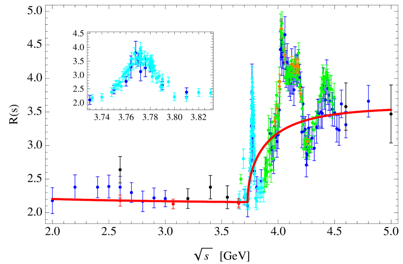
Figure 1: Data for the ratio $R$ for $e^{+}e^{-}\rightarrow$ hadrons in the charm threshold region: Crystal Ball CB86 (green) [34]; BES00, 02, 06, 09 (black, blue, cyan, and red) [35, 36, 37, 38], and CLEO09 (orange) [39]. The full (red) curve shows $R_{c}^{\rm Cont}(s)$ with $\lambda_{3}^{c}=1.23$ and $\hat{m}_{c}(\hat{m}_{c})=1.272$GeV. The inner plot is a zoom-in into the energy range $2M_{D^{0}}\leq\sqrt{s}\leq 3.83$ GeV.

2.1 Uncertainty estimate

In order to determine an error for the continuum contributions we proceed in the following way [15]: instead of using Eqs. (2, 15), we can compare experimental data shown in Fig. 1 with the zeroth moment in the restricted energy range of the threshold region, $2M_{D^{0}}\leq\sqrt{s}\leq 4.8$ GeV to obtain an experimental value for $\lambda_{3}^{c}$, denoted $\lambda_{3}^{c,{\rm exp}}$. Here we fix $\hat{m}_{c}(\hat{m}_{c})$ using Eq. (15) and proceed to solve Eq. (2) by comparing with ${\cal M}_{0}^{\rm exp}$. Then we can also determine an error, $\Delta\lambda_{3}^{c,{\rm exp}}$ from the experimental uncertainty of the data in this threshold region.

We calculate the experimental moments via numerical integrals over the available experimental data, cf. Fig. 1. Experimental data is classified in five different intervals, see Fig. 2, which allow us to fully take into account correlated and uncorrelated uncertainties among different collaborations and intervals. The results for the experimental moments in the threshold region, $2M_{D^{0}}\leq\sqrt{s}\leq 4.8$ GeV are given in Table 2.1. For the results in the columns labeled ’Data’, light-quark contributions have been subtracted using the pQCD prediction at order ${\cal O}(\hat{\alpha}_{s}^{3})$, see Ref. [15]. Its second column shows the required value for $\lambda_{3}^{c,{\rm exp}}$ such that the zeroth moment sum rule is experimentally satisfied after fixing $\hat{m}_{c}(\hat{m}_{c})=1.272$GeV. The rest of the moments in this column are reported to show the consistency of the approach. Even for the highest moments, the consistency is very good. The last column collects, for comparison, the value for the moments in the same energy region using $\lambda_{3}^{c}=1.23$ extracted from the theoretical determination.

The shift in the moments resulting from the different values for $\lambda_{3}^{c}$ (either from two moments combined with resonance data only, or from the comparison of the 0th moment with continuum data in the threshold region) turns out to be small. Strictly speaking this shift is a one-sided error, but to be conservative we include it as an additional error in the results of Table 2.1. A graphical account of this shift is shown in Fig. 3 as a cyan band for the result of the $0{\rm th}+2{\rm nd}$ moments pair for $\hat{m}_{c}(\hat{m}_{c})=1.272$GeV. In this case, $\lambda_{3}^{c,{\rm exp}}=1.34(17)$, c.f. Table 2.1. The red solid curve corresponds to the same pair of moments and the same quark mass with $\lambda_{3}^{c}=1.23$, and well overlaps with the cyan band.

Contributions to the charm moments ($\times 10^{n}\,\mbox{GeV}^{2n}$) from the energy range $2M_{D^{0}}\leq\sqrt{s}\leq 4.8$ GeV. For the results in the columns labeled ’Data’, light-quark contributions have been subtracted using the pQCD prediction at order ${\cal O}(\hat{\alpha}_{s}^{3})$. The entries here are obtained from the separate contributions shown in Fig. 2 taking into account the correlation of systematic errors within each experiment. The third column uses $\hat{m}_{c}=1.272{\rm GeV}$ and $\lambda_{3}^{c,{\rm exp}}$ determined by the zeroth experimental moment (see text for details). The last column shows the theoretical prediction for the moments using $\hat{m}_{c}=1.272{\rm GeV}$ and $\lambda^{c}_{3}=1.23$. $n$ Data $\lambda^{c}_{3}=1.34(17)$ $\lambda^{c}_{3}=1.23$ 0 0.6367(195) 0.6367(195) 0.6239 1 0.3500(101) 0.3509(111) 0.3436 2 0.1957(54) 0.1970(65) 0.1928 3 0.1111(29) 0.1127(38) 0.1102 4 0.0641(16) 0.0657(23) 0.0642 5 0.0375(9) 0.0389(14) 0.0380

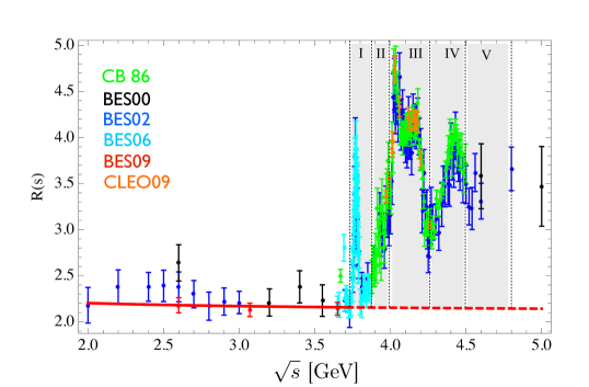
Figure 2: Data for the ratio $R$ for $e^{+}e^{-}\rightarrow$ hadrons in the charm threshold region: Crystal Ball CB86 (green) [34]; BES00, 02, 06, 09 (black, blue, cyan, and red) [35, 36, 37, 38], and CLEO09 (orange) [39]. The gray bands indicate the five intervals considered for evaluating the experimental moments.

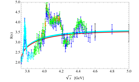
Figure 3: Data for the ratio $R$ for $e^{+}e^{-}\rightarrow$ hadrons in the charm threshold region: Crystal Ball CB86 (green) [34]; BES00, 02, 06, 09 (black, blue, cyan, and red) [35, 36, 37, 38], and CLEO09 (orange) [39]. The full (red) curve shows $R_{c}^{\rm Cont}(s)$ with $\lambda_{3}^{c}=1.23$ and $\hat{m}_{c}(\hat{m}_{c})=1.272$GeV and the cyan band shows $R_{c}^{\rm Cont}(s)$ with $\hat{m}_{c}(\hat{m}_{c})=1.272$GeV and $\lambda_{3}^{c,{\rm exp}}=1.34(17)$ .

Finally, we assign a truncation error to the theory prediction of the moments following the method proposed in Ref. [16] which considers the largest group theoretical factor in the next uncalculated perturbative order as a way to estimate errors,

$$\Delta{\cal M}_{n}^{(i)}=\pm Q_{q}^{2}N_{C}C_{F}C_{A}^{i-1}\,\left(\frac{\hat{\alpha}_{s}(\hat{m}_{q})}{\pi}\right)^{i}\left(\frac{1}{2\hat{m}_{q}(\hat{m}_{q})}\right)^{2n}$$ (18)

($N_{C}=C_{A}=3$, $C_{F}=4/3$). At order ${\cal O}(\hat{\alpha}_{s}^{4})$, this corresponds to an uncertainty of $\pm 48(\hat{\alpha}_{s}/\pi)^{4}$ for $\hat{C}_{n}^{(4)}$ in Eq. (15).

For the moments with $n>3$ taken from Ref. [30] we have to include additional uncertainties specific to the method used to obtain predictions for ${\cal M}_{n}$. These errors are very small, but included for completeness.

The charm mass and the continuum parameter $\lambda_{3}^{c}$ can, in principle, be determined from any combination of two moments, not only $0{\rm th}+2{\rm nd}$. The zeroth moment, however, is expected to provide the highest sensitivity. The results for combinations of the zeroth with one higher moment are summarized in Table 2.1 and visualized in Fig. 4. We include the difference between the two possibilities to determine $\lambda_{3}^{c}$ as described above as an additional error.

As an example on how to understand Table 2.1, select the $0{\rm th}+2{\rm nd}$ moments pair as the result for the quark mass, we would combine the total error $7.8$ MeV with $0.37\times 14$ MeV error from the condensate uncertainty and with $2.6\times 1.6$ MeV from $\hat{\alpha}_{s}(M_{z})=0.1182(16)$ [18]. Then, $\hat{m}_{c}(\hat{m}_{c})=1272(9)$MeV. Doing so for each pair of moments collected in the table, we notice that the combination $0{\rm th}+2{\rm nd}$ provides the smallest total error for the heavy quark mass. Let us remark that for the highest moments, the truncation of the OPE series, i.e. condensates of higher dimension not considered in our approach can be important [15]. While difficult to assert, we belief that these higher dimension condensates are well included in our condensate error estimate. However, to be on the safe side, charm quark mass determination using the fourth and fifth moment sum rules may have an underestimated error. They should not be considered. On the contrary, the zeroth and first moments are the ones less sensitive to the OPE truncation with the combination $0{\rm th}+1{\rm st}$ being a most favorable choice. However, this combination is the one most sensitive to the continuum region, with largest shift in $\lambda_{3}^{c,{\rm exp}}$, cf. Table  2.1. The pair of the zeroth and second moments is our optimal choice since balance well between reduced effects of the OPE series truncation and good description of the continuum region. This pair has also the smallest total uncertainty in the charm mass determination.

Values of $\hat{m}_{c}(\hat{m}_{c})$ and $\lambda_{3}^{c}$ determined from different pairs of moments and split-up of the errors for the charm mass. The errors denoted ’Total’ are the quadratic sum of the two errors from $\lambda_{3}$, the one from the resonances and the truncation error. Errors induced by the uncertainties of $\hat{\alpha}_{s}$ and of $\langle\frac{\hat{\alpha}_{s}}{\pi}G^{2}\rangle$ (in units of GeV⁴) are parametric and are given separately in the last two lines. $\Delta\hat{m}_{c}(\hat{m}_{c})~{}[\mbox{MeV}]$ ${\cal M}_{0}$ – ${\cal M}_{1}$ ${\cal M}_{0}$ – ${\cal M}_{2}$ ${\cal M}_{0}$ – ${\cal M}_{3}$ ${\cal M}_{0}$ – ${\cal M}_{4}$ ${\cal M}_{0}$ – ${\cal M}_{5}$ $\hat{m}_{c}(\hat{m}_{c})~{}[\mbox{MeV}]$ 1280.9 1272.4 1269.1 1265.8 1262.2 $\lambda_{3}^{c}$ 1.154 1.230 1.262 1.291 1.323 $\lambda_{3}^{c,{\rm exp}}({\cal M}_{0})$ 1.35(17) 1.34(17) 1.34(17) 1.33(17) 1.32(17) Resonances 5.8 4.5 3.9 3.3 2.8 Truncation error 6.3 5.9 7.2 8.9 10.5 Shift of $\lambda_{3}^{c}$ +6.4 +1.5 +0.3 +0.1 +0.1 $\Delta\lambda_{3}^{c,{\rm exp}}$ 4.7 1.7 0.7 0.3 0.2 Total: 11.7 7.8 8.2 9.5 10.9 $10^{3}\times$Condensates $-0.25\langle\frac{\hat{\alpha}_{s}}{\pi}G^{2}\rangle$ $-0.37\langle\frac{\hat{\alpha}_{s}}{\pi}G^{2}\rangle$ $-0.54\langle\frac{\hat{\alpha}_{s}}{\pi}G^{2}\rangle$ $-0.73\langle\frac{\hat{\alpha}_{s}}{\pi}G^{2}\rangle$ $-0.88\langle\frac{\hat{\alpha}_{s}}{\pi}G^{2}\rangle$ (-1.3 MeV) (-1.9 MeV) (-2.7 MeV) (-3.7 MeV) (-4.4 MeV) $10^{3}\times\Delta\hat{\alpha}_{s}(M_{z})$ $+3.6\Delta\hat{\alpha}_{s}$ $+2.6\Delta\hat{\alpha}_{s}$ $+1.6\Delta\hat{\alpha}_{s}$ $+0.6\Delta\hat{\alpha}_{s}$ $-0.4\Delta\hat{\alpha}_{s}$ (+5.8 MeV) (+4.2 MeV) (+2.6 MeV) (+1.0 MeV) (-0.6 MeV)

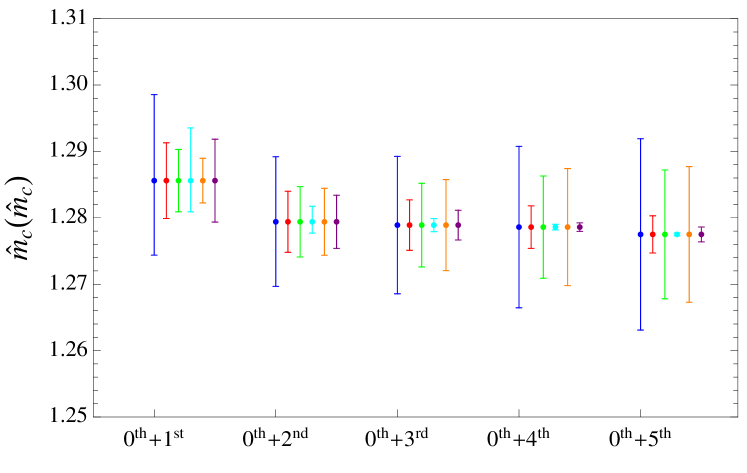
Figure 4: $\hat{m}_{c}(\hat{m}_{c})$ using different combinations of moments and the error budget for each combination. Blue is the full error, red is the one from the resonance region, green from the truncation errors of the theoretical moments, cyan from the error of $\lambda_{3}^{c}$ (which is the combination of the shift and the experimental error on $\lambda_{3}^{c}$), orange from the gluon condensate and purple from the uncertainty of $\Delta\hat{\alpha}_{s}(M_{z})$.

In Ref. [16], a determination of the heavy quark mass at ${\cal O}(\hat{\alpha}_{s}^{2})$ was performed requiring as well self-consistency between the $0{\rm th}+2{\rm nd}$ moments to constrain the continuum region. The main difference between the results in Ref. [16] and the ones presented here can be summarized as follows:

• The theoretical sum rules are considered at order ${\cal O}(\hat{\alpha}_{s}^{3})$, including the expression for $\lambda_{3}^{q}(s)$ and the theoretical moments.

• The electronic widths of the narrow-width resonance states are measured now with higher precision. Actually, the shift in their central values amount to $1\sigma$ and induce the largest shift in the quark mass determination when comparing Table 2.1 with Ref. [16].

• The experimental determination of $\hat{\alpha}_{s}(M_{z})$, i.e., the value $\hat{\alpha}_{s}(M_{z})=0.1182(16)$ used in this work has been improved with respect to the one used in Ref. [16].

• Other minor improvements include more experimental data in the continuum region and better determination of the condensate contribution.

3 Conclusions

In this paper we presented a determination of the charm quark mass based on the work of Ref. [15]. We revisit there the method of relativistic sum rules with emphasis on the evaluation of the uncertainty. By invoking the zeroth sum rule and requiring self-consistency with higher-moment sum rules, we can show that the overall error may be constrained within the approach.

After considering the combination of two different sum rules, the only experimental information required are the masses and electronic decay widths of the narrow resonances in the sub-continuum charm region, $J/\Psi(1S)$ and $\Psi(2S)$. Comparison with experimental data in this region is later on used to check the results and determine an experimental error.

The results reported here are preliminary and more details are provided in Ref. [15].

References

- [1] A. Laschka, N. Kaiser, and W. Weise. Phys. Rev. D, 83, 094002, 2011.
- [2] Y. Namekawa et al. Phys. Rev. D, 84, 074505, 2011.
- [3] J. Heitger, G. M. von Hippel, S. Schaefer, and F. Virotta. PoS, LATTICE2013, 475, 2014.
- [4] N. Carrasco et al. Nucl. Phys. B, 887, 19, 2014.
- [5] B. Chakraborty, C. T. H. Davies, B. Galloway, P. Knecht, J. Koponen, G. C. Donald, R. J. Dowdall, G. P. Lepage, and C. McNeile. Phys. Rev. D, bf 91, 054508 , 2015.
- [6] S. Alekhin, J. Blumlein, and S. Moch. Phys. Rev. D, 89, 054028, 2014.
- [7] H. Abramowicz et al. Eur. Phys. J. C, 73, 2311, 2013.
- [8] V. A. Novikov, L. B. Okun, Mikhail A. Shifman, A. I. Vainshtein, M. B. Voloshin, and Valentin I. Zakharov. Phys. Rept., 41, 1, 1978.
- [9] M. A. Shifman, A. I. Vainshtein, and V. I. Zakharov. Nucl. Phys. B, 147, 385, 1979.
- [10] M. A. Shifman, A. I. Vainshtein, and V. I. Zakharov. Nucl. Phys. B, 147, 448, 1979.
- [11] K. Chetyrkin, J. H. Kuhn, A. Maier, P. Maierhofer, P. Marquard, M. Steinhauser, and C. Sturm. Theor. Math. Phys., 170, 217, 2012.
- [12] B. Dehnadi, A. H. Hoang, V. Mateu, and S. M. Zebarjad. JHEP, 09, 103, 2013.
- [13] S. Bodenstein, J. Bordes, C. A. Dominguez, J. Penarrocha, and K. Schilcher. Phys. Rev. D, 83, 074014 , 2011.
- [14] S. Narison. Phys. Lett. B, 707, 259, 2012.
- [15] J. Erler, P. Masjuan and H. Spiesberger, arXiv:1610.08531 [hep-ph].
- [16] J. Erler and M.-X. Luo. Phys. Lett. B, 558, 125, 2003.
- [17] K. G. Chetyrkin, R. V. Harlander, and J. H. Kuhn. Nucl. Phys. B, 586, 56, 2000.
- [18] K. A. Olive et al. Chin. Phys. C, 38, 090001, 2014.
- [19] F. Jegerlehner. http://www-com.physik.hu-berlin.de/{~}fjeger/.
- [20] K. G. Chetyrkin, J. H. Kuhn, and M. Steinhauser. Nucl. Phys. B, 482, 213, 1996.
- [21] K. G. Chetyrkin, B. A. Kniehl, and M. Steinhauser. Nucl. Phys. B, 510, 61, 1998.
- [22] Y. Kiyo, A. Maier, P. Maierhofer, and P. Marquard. Nucl. Phys. B, 823, 269, 2009.
- [23] A. H. Hoang, V. Mateu, and S. M. Zebarjad. Nucl. Phys. B, 813, 349, 2009.
- [24] K. G. Chetyrkin, J. H. Kuhn, and C. Sturm. Eur. Phys. J. C, 48, 107, 2006.
- [25] R. Boughezal, M. Czakon, and T. Schutzmeier. Phys. Rev. D, 74, 074006 , 2006.
- [26] A. Maier, P. Maierhofer, and P. Marqaurd. Phys. Lett. B, 669, 88, 2008.
- [27] A. Maier, P. Maierhofer, P. Marquard, and A. V. Smirnov. Nucl. Phys. B, 824, 1, 2010.
- [28] K. G. Chetyrkin, J. H. Kuhn, and M. Steinhauser. Nucl. Phys. B, 505, 40, 1997.
- [29] A. Maier, P. Maierhofer, and P. Marquard. Nucl. Phys. B, 797, 218, 2008.
- [30] D. Greynat, P. Masjuan, and S. Peris. Phys. Rev. D, 85, 054008, 2012.
- [31] D. J. Broadhurst, P. A. Baikov, V. A. Ilyin, J. Fleischer, O. V. Tarasov, and V. A. Smirnov. Phys. Lett. B, 329, 103, 1994.
- [32] J. H. Kuhn, M. Steinhauser, and C. Sturm. Nucl. Phys. B, 778, 192, 2007.
- [33] C. A. Dominguez, L. A. Hernandez, K. Schilcher, and H. Spiesberger. JHEP, 03, 053, 2015.
- [34] A. Osterheld, R. Hofstadter, R. Horisberger, I. Kirkbride, H. Kolanoski, et al. Submitted to: Phys. Rev. D, 1986.
- [35] J. Z. Bai et al. Phys. Rev. Lett., 84, 594, 2000.
- [36] J. Z. Bai et al. Phys. Rev. Lett., 88, 101802, 2002.
- [37] M. Ablikim, J. Z. Bai, Y. Ban, J. G. Bian, X. Cai, et al. Phys. Rev. Lett., 97, 262001, 2006.
- [38] M. Ablikim et al. Phys. Lett. B, 677, 239, 2009.
- [39] D. Cronin-Hennessy et al. Phys. Rev. D, 80, 072001, 2009.