Scalar QCD at nonzero density

Abstract:

We study scalar QCD at nonzero density in the strong coupling limit. It has a sign problem which looks structurally similar to the one in QCD. We show first data for the reweighting factor. After introducing dual variables by integrating out the SU(3) gauge links, we find that at least 3 flavors are needed for a nontrivial dependence on the chemical potential. In this dual representation there is no sign problem remaining. The dual variables are partially constrained, thus we propose to use a hybrid approach for the updates: For unconstrained variables local updates can be used, while for constrained variables using updates based on the worm algorithm is more promising.

1 Introduction

Lattice QCD is one of the most important tools for studying the nonperturbative as well as thermodynamic aspects of QCD from first principles. However, if we introduce a chemical potential $\mu$ in order to explore the phase-diagram of QCD at nonzero density, the standard approach fails due to the sign problem, that is, the weights of the gauge configurations (having integrated out the quarks) become complex and therefore ill-suited for importance sampling in Monte-Carlo simulations.

There have been many proposals to remedy this shortcomming. Standard reweighting techniques fail because the reweighting factor rapidly approaches zero in the interesting regime around the critical chemical potential $\mu_{c}$. Another proposal has been the MDP-formulation (Monomer-Dimer-Polymer) of strong coupling QCD [1, 2]. There first the gauge links and after that the fermion fields are integrated out. This leaves a constrained spin system of occupation numbers or dual variables. However, even then there is still a sign problem remaining, even though it is rather mild [3].

In these proceedings we consider a scalar version of QCD in the strong coupling limit (scSQCD), where instead of fermionic fields we use complex scalar fields. We can couple a chemical potential to the conserved charge of the scalar fields, which also results in a complex action. We dualize the theory in a similar way to the MDP-formulation, which solves the sign problem. Afterwards we discuss the diagrammatic representation of the dual theory and propose a simulation strategy for it.

2 Strong coupling scalar QCD

The action for this model reads

$$S =\sum_{x}\sum_{f=1}^{N_{f}}\left(\sum_{\nu=1}^{d}\left(e^{\mu\delta_{\nu,\hat{0}}}\phi_{x}^{(f)\dagger}U_{x,\nu}\phi_{x+\hat{\nu}}^{(f)}+e^{-\mu\delta_{\nu,\hat{0}}}\phi_{x+\hat{\nu}}^{(f)\dagger}U_{x,\nu}^{\dagger}\phi_{x}^{(f)}-2\phi_{x}^{(f)\dagger}\phi_{x}^{(f)}\right)-m^{2}\phi_{x}^{(f)\dagger}\phi_{x}^{(f)}\right)$$ (1)

where $\phi$ is the complex scalar field, $U$ the SU(3) gauge field, $N_{f}$ the number of flavors and $d$ the number of spacetime dimensions.

For $\mu\neq 0$ the action becomes complex and we end up with a sign problem. In figure 1 the (phase-quenched) reweighting factor, $r=\langle(|\det M|/\det M)^{N_{F}}\rangle$, is plotted as a function of the chemical potential $\mu$. Above $\mu=0.7$ it decreases rapidly. Figure 2 shows that $r=e^{-\Delta fV}$ obeys the correct volume dependence, where $\Delta f$ is the free energy density. Further we note that $\Delta f$ seems to have an exponential increase/decrease with $\mu$. A naive extrapolation gives a maximal free energy density of $\Delta f(\mu_{\times})=2.04(7)$ at $\mu_{\times}=1.172(2)$. This means that the reweighting factor becomes smaller than $10^{-14}$ already for a $4\times 4$ lattice. Therefore it is unfeasible to simulate the region around $\mu_{c}$ by reweighting.

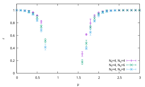
Figure 1: The reweighting factor is plotted as a function of $\mu$. The data is from 10000 configurations and we set $N_{f}=3,m=0.1$. For $\mu\in[0.7,1.6]$ the autocorrelationtime becomes so large that neither the errors nor the mean values are reliable any more. Therefore we have omitted the data points in this region.

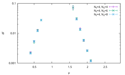
Figure 2: The free energy density $\Delta f$, $r=e^{-\Delta fV}$, is plotted as a function of $\mu$. A naive extrapolation yields a crossing point at $\mu_{\times}=1.172(2)$, with a free energy density of $\Delta f_{\times}=2.04(7)$.

3 Dualization

In order to proceed to dualize the theory, we rewrite the action:

$$S =\sum_{x}\left(\sum_{\nu}\mathrm{Tr}\,\left(J_{x,\nu}U_{x,\nu}+K_{x,\nu}U_{x,\nu}^{\dagger}\right)-\sum_{f}\left((2d+m^{2})\phi_{x}^{(f)\dagger}\phi_{x}^{(f)}\right)\right)$$ (2)

$$J_{x,\nu} =e^{\mu\delta_{\nu,\hat{0}}}\sum_{f}\phi_{x+\hat{\nu}}^{(f)}\phi_{x}^{(f)\dagger}\hskip 30.00005pt\mathrm{forward\ hopping}$$ (3)

$$K_{x,\nu} =e^{-\mu\delta_{\nu,\hat{0}}}\sum_{f}\phi_{x}^{(f)}\phi_{x+\hat{\nu}}^{(f)\dagger}\hskip 27.0pt\mathrm{backward\ hopping}$$ (4)

For the partition function $Z$ we have to integrate over the gauge field $U$ as well as the scalar fields $\phi$:

$$Z =\int\mathcal{D}\phi\mathcal{D}\phi^{\dagger}\int\mathcal{D}U\,e^{S}.$$ (5)

The SU(3) integral at a single bond $(x,\nu)$ can be turned into a five-fold sum, see, e.g., [4]:

$$\int_{\mathrm{SU(3)}}dU\,\exp(\mathrm{Tr}\,(JU+KU^{\dagger}))=\sum_{j,k,l,n,\bar{n}=0}^{\infty}\frac{X^{j}}{j!}\frac{Y^{k}}{k!}\frac{Z^{l}}{l!}\frac{\Delta^{n}}{n!}\frac{\bar{\Delta}^{\bar{n}}}{\bar{n}!}\frac{2}{f^{(1)}!f^{(2)}!}$$ (6)

where $f^{(1)}$ and $f^{(2)}$ are shorthands for

$$f^{(1)}=k+2l+n+\bar{n}+1\hskip 30.00005ptf^{(2)}=j+2k+3l+n+\bar{n}+2,$$ (7)

and $X,Y,Z,\Delta,\bar{\Delta}$ are functions of $J,K$:

$$X =\mathrm{Tr}\,(KJ) Y =\frac{1}{2}\left[X^{2}-\mathrm{Tr}\,((KJ)^{2})\right] Z =\det(KJ)$$ (8)

$$\Delta =\det J \bar{\Delta} =\det K$$ (9)

We can apply (6) to each bond separately because the SU(3) integrals factorize. Then the partition function becomes

$$Z =\sum_{\{j,k,l,n,\bar{n}\}}\int\mathcal{D}\phi\mathcal{D}\phi^{\dagger}\rho(|\phi|)\prod_{x,\nu}2\frac{X^{j_{x,\nu}}_{x,\nu}Y^{k_{x,\nu}}_{x,\nu}Z^{l_{x,\nu}}_{x,\nu}\Delta^{n_{x,\nu}}_{x,\nu}\bar{\Delta}^{\bar{n}_{x,\nu}}_{x,\nu}}{j_{x,\nu}!k_{x,\nu}!l_{x,\nu}!n_{x,\nu}!\bar{n}_{x,\nu}!f^{(1)}_{x,\nu}!f^{(2)}_{x,\nu}!}$$ (10)

$$\rho(|\phi|) =\prod_{x,f}e^{-(2d+m^{2})|\phi^{(f)}_{x}|^{2}}$$ (11)

Thus we are left with the integration over the scalar fields, which are gaussian distributed, and the summation over configurations of dual variables $j,k,l,n,\bar{n}$.

The functions $X,Y,Z$ only depend on the matrix $KJ$. In our case the $\mu$ dependence cancels, cf. (3) and (4), and we have $KJ=J^{\dagger}J$, which is a positive operator, and hence $X,Y,Z$ are positive as well. However, $\Delta,\bar{\Delta}$ are complex in general. One can work out that

$$\Delta_{x,\nu} =e^{3\mu\delta_{\nu,0}}\sum_{\sigma}\phi^{(\sigma(1))}_{x+\hat{\nu}}\cdot\left(\phi^{(\sigma(2))}_{x+\hat{\nu}}\times\phi^{(\sigma(3))}_{x+\hat{\nu}}\right)\left(\phi^{(\sigma(1))}_{x}\cdot\left(\phi^{(\sigma(2))}_{x}\times\phi^{(\sigma(3))}_{x}\right)\right)^{*}$$ (12)

$$\bar{\Delta}_{x,\nu} =e^{-3\mu\delta_{\nu,0}}\sum_{\sigma}\phi^{(\sigma(1))}_{x}\cdot\left(\phi^{(\sigma(2))}_{x}\times\phi^{(\sigma(3))}_{x}\right)\left(\phi^{(\sigma(1))}_{x+\hat{\nu}}\cdot\left(\phi^{(\sigma(2))}_{x+\hat{\nu}}\times\phi^{(\sigma(3))}_{x+\hat{\nu}}\right)\right)^{*}$$ (13)

where $\sigma$ runs over all maps $\sigma:\{1,2,3\}\to\{1,\dots,N_{f}\}$ with $\sigma(1)<\sigma(2)<\sigma(3)$. This means that for $N_{f}<3$ there is no $\mu$ dependence since then $\Delta\equiv\bar{\Delta}\equiv 0$, see also [5]. In the following we restrict ourselves to the first nontrivial case, $N_{f}=3$. However, the result is valid also for $N_{f}>3$.

To tackle the remaining sign problem, note that the partition function involves gaussian integrations of the form

$$\int d\phi d\phi^{*}\,e^{-|\phi|^{2}}(\phi)^{a}(\phi^{*})^{b} \sim\delta_{ab}$$ (14)

at each site for each flavor and color. Thus the only contribution to the partition function comes from terms where the power of $\phi$ at a site matches that of $\phi^{*}$.

$X,Y,Z$ satisfy the constraint at a single bond, however, $\Delta,\bar{\Delta}$ do not. From (14) one can see that only closed loops of $\Delta,\bar{\Delta}$ satisfy the constraint. For such a closed loop $C$ the weight is proportional to

$$w(C) \sim e^{3N_{t}\mu w_{t}}\prod_{(x,\hat{\nu})\in C}\phi^{(1)}_{x}\cdot\left(\phi^{(2)}_{x}\times\phi^{(3)}_{x}\right)\left(\phi^{(1)}_{x+\hat{\nu}}\cdot\left(\phi^{(2)}_{x+\hat{\nu}}\times\phi^{(3)}_{x+\hat{\nu}}\right)\right)^{*}$$ (15)

$$=e^{3N_{t}\mu w_{t}}\prod_{x\in C}\left|\phi^{(1)}_{x}\cdot\left(\phi^{(2)}_{x}\times\phi^{(3)}_{x}\right)\right|^{2}\geq 0,$$ (16)

where $w_{t}$ is the winding number in the temporal direction. So we have to consider only closed loop configurations in the partition function. Then there is no sign problem remaining even at $\mu\neq 0$.

4 Discussion and Conclusion

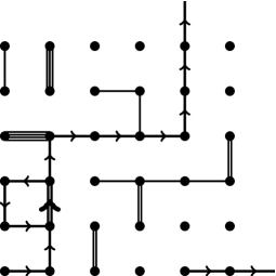
Figure 3: A sample configuration of the dual variables. Bonds can be occupied arbitrarily with the dual variables $j,k,l,n,\bar{n}$, the only constraint being that the $n,\bar{n}$ have to form closed loops. Since these loops are directional, they are marked with arrows. Note that in constrast to the MDP-formulation there is also no restriction of baryonic bonds ($n,\bar{n}$) being disjunct from mesonic bonds ($j,k,l$) and sites without occupied bonds are possible as well. Also there is no restriction on the occupation numbers, they can, in principle, be arbitrarily large. However, large values are surpressed by the factorials in the denominator of eq. (3.9).

The configurations of the dual variables can be represented diagrammatically in a similar way to the MDP-formulation, see figure 3. We may call closed loops of $n,\bar{n}$ baryonic, since they are directional, and couple to the chemical potential $\mu$. The other dual variables $j,k,l$ we call mesonic. A notable difference to the MDP-formulation is that in our case there is no restriction of mesonic bonds being disjunct from baryonic ones. Also, since we are in a bosonic theory, there is no restriction on the dual variables. In principle they can run from $0$ to $\infty$, however, large values are strongly suppressed by the factorials in the denomitator of (10).

From the derivation of the original MDP-formulation it is evident that there the remaining sign problem stems from the fermionic nature of the fields. In particular, there the sign problem comes from the anticommutation rules, the staggered phases, the backward hoppings, and the antiperiodic boundary conditions in the time direction. In the scalar case all these causes are absent, and as we have seen this results in a dual theory that has no sign problem.

For the simulation of this model we propose a hybrid strategy. The dual variables $j,k,l$ can be updated via a local metropolis step, which involves an evaluation of the functions $X,Y,Z$ on the corresponding bond, as $X,Y,Z$ are all positive. The $n,\bar{n}$ can be updated using a worm-type of algorithm. To that end one can use the fact that for a closed loop the contribution of each site is positive, see eq. (16), and one can use a heat-bath method to decide which way to go with the worm. Finally the (gaussian distributed) scalar fields $\phi,\phi^{\dagger}$ can also be updated via a local metropolis step by evaluating $X,Y,Z$ on the adjacent bonds as well as the contribution of the closed $n,\bar{n}$-loops to that particular site, cf. eq. (16). We leave numerical simulations which explore the phase diagram of this model for future publications.

We thank Jacques Bloch for helpful discussions. This work is supported by the DFG-grants BR 2872/6-1 & 2872/7-1.

References

- [1] P. Rossi, U. Wolff, Lattice QCD With Fermions at Strong Coupling: A Dimer System, Nucl. Phys. B248, (1984), p105-122
- [2] F. Karsch, K. H. Mutter, Strong coupling QCD at finite baryon number density, Nucl. Phys. B313 (1989) p541-559, CERN-TH-5063/88
- [3] M. Fromm, Lattice QCD at strong coupling, (2010), ETH-19297, http://e-collection.library.ethz.ch/view/eth:2616
- [4] K. E. Eriksson, N. Svartholm, B. S. Skagerstam, On Invariant Group Integrals in Lattice QCD, J. Math. Phys. 22 (1981) 2276, CERN-TH-2974
- [5] U. Wolff, The SU() Lattice Higgs Model at Strong Gauge Coupling, Nucl. Phys. B280 (1987), p680-688, DESY-86-085