Engineering electronic states of periodic and quasiperiodic chains by buckling

Abstract

The spectrum of spinless, non-interacting electrons on a linear chain that is buckled in a non-uniform, quasiperiodic manner is investigated within a tight binding formalism. We have addressed two specific cases, viz., a perfectly periodic chain wrinkled in a quasiperiodic Fibonacci pattern, and a quasiperiodic Fibonacci chain, where the buckling also takes place in a Fibonacci pattern. The buckling brings distant neighbors in the parent chain to close proximity, which is simulated by a tunnel hopping amplitude. It is seen that, in the perfectly ordered case, increasing the strength of the tunnel hopping (that is, bending the segments more) absolutely continuous density of states is retained towards the edges of the band, while the central portion becomes fragmented and host subbands of narrowing widths containing extended, current carrying states, and multiple isolated bound states formed as a result of the bending. A switching “on” and “off” of the electronic transmission can thus be engineered by buckling. On the other hand, in the second example of a quasiperiodic Fibonacci chain, imparting a quasiperiodic buckling is found to generate continuous subband(s) destroying the usual multifractality of the energy spectrum. We present exact results based on a real space renormalization group analysis, that is corroborated by explicit calculation of the two terminal electronic transport.

I Introduction

Localization of single particle quantum states has been an ubiquitous phenomenon, observed primarily as a consequence of disorder in a system, and is traditionally called the Anderson localization anderson . The pivotal result in the field of disorder-induced localization is that, the single particle eigenstates of a Hamiltonian describing a disordered lattice should be exponentially localized for dimension $d\leq 2$, and even for $d>2$ for strong disorder. The effect is strongest in one dimension where all the states are localized for any strength of disorder. The envelope of the wave function decays exponentially with respect to a given location in the lattice  kramer ; abrahams . These results have been aptly justified by various calculations related to the localization length rudo1 ; rudo2 and the density of states alberto . The single parameter scaling hypothesis – its validity rudo3 , variance deych , or even violation bunde ; titov in low dimensional systems within a tight-binding approximation has also enriched the field.

This picture is to be contrasted with the effect of quasiperiodic order  kohmoto1 ; kohmoto2 in one dimensional lattices where the single particle excitations are critical and exhibit a power law localization with a multifractal character in general  mace . Resistance for such systems exhibits power law growth as well as the size of the lattice increases kohmoto3 ; sankar ; macia . The exotic spectral properties of quasiperiodic lattices occupied an immense volume of literature over the past three decades, and even today, the unusual behaviour of quantum conductance in such systems are of immense inetrest varma .

In this communication, we revisit the effect of ‘deterministic disorder’, introduced in an infinitely long one dimensional chain of atomic sites by buckling the chain in local segments, and throughout its length, following a quasiperiodically ordered sequence. Bent quantum wires have been studied previously in the context of ballistic transport characteristics vacek . Single and multiply bent two dimensional quantum wires were examined in respect of localized, doubly split one electron states vakhnenko . Apart from these, winding chains have been considered as models of conducting polymers xiong1 ; xiong2 . The winding brings sites that were distant neighbors in the unperturbed system to close proximity, and a tunnel hopping provides additional paths for the electron. The lattice becomes a topologically disordered (deterministic though) system in the spirit of Guinea and Vergés guinea , who discussed the effect of fluctuating coordination numbers in a linear chain, caused by dangling branches coupled from a side, or bridging two distant sites in a one dimensional lattice. Such tunneling has been shown xiong1 ; xiong2 to have profound influence on quantum transport, leading to large localization lengths in disordered polymers, which is indicative of a metal-insulator (MI) transition in such systems. Real polymers of course, include interaction between different constituent chains, the coupling between the adjacent chains being mediated by the overlapping hydrogen orbitals. In several cases the main spectral features can be explained by an effective tight binding model with next nearest neighbor hopping integrals. The effect of second neighbor hopping is also studied for quasi one dimensional organic polymer ferromagnetic systems and have unravelled a plethora of information  kailun . Buckling a chain makes such longer range interactions possible in a natural way, and thus deserves close scrutiny.

In addition, a quasiperiodic order in chains and their bending are two important ingredients that have been shown to arise in the recent field of two dimensional materials, a graphene nanoribbon for example naumis . This provides an extra motivation for studying the present model.

We examine two different cases. At first, we consider a perfectly periodic chain of atoms within a tight binding approximation. Buckling is introduced in a Fibonacci quasiperiodic sequence kohmoto1 such that the chain bends after every $n$ and $m$ atoms, the numbers $n$ and $m$ being distributed in a Fibonacci pattern. Tunnel hopping is introduced across such clusters and it is seen that for large strength of the tunnel hopping amplitude, which may be thought to be caused by large bending of the local segments, the energy spectrum turns out to be extremely interesting. The outer edges of the spectrum retain the character of a pure, one dimensional chain of atoms, while the central part, spanning between $E=\epsilon\pm 2t$, feels the ‘disorder’ and breaks up into multiple subbands populated by extended eigenstates as well as sharply localized bound states. Thus wrinkling the chain appropriately one can look into the possibility of a switching action as one sweeps the Fermi energy from the domain of absolutely continuous spectrum to the fragmented one, mixed with transparent and localized states.

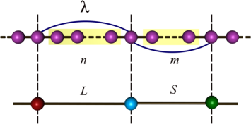
Figure 1: (Color online) A one-dimensional chain of atoms with identical quantum dots each of having on-site potentials $\epsilon$ and hopping integral $t$ with long range hopping $\lambda$ (blue line) across $n$-atoms and across $m$-atoms which follow a Fibonacci sequence, as discussed in text. The figure below indicates the renormalized version of the buckled ordered chain with restricted long range hopping.

In the second example, we consider a quasiperiodic Fibonacci chain to begin with. The tunnel hopping, spanning the second neighbors, but in a restricted sense, also follows a Fibonacci sequence. This introduces a competing quasiperiodic order. The introduction of the tunnel hopping in this case results in something totally different. We have encountered several cases where an appropriate choice of the tunnel hopping is seen to generate absolutely continuous subbands in the otherwise fragmented Cantor set energy spectrum, typical of a Fibonacci lattice kohmoto1 making the system conduct over specified energy intervals.

In what follows, we discuss our findings in details. In section II we lay down the models and the methods followed. Section III contains the results for both the cases addressed here, and in section IV we draw our conclusions.

II The model and the method

II.1 The perfectly periodic chain with quasiperiodic buckling

Let us refer to Fig. 1 which shows a linear chain of atomic scatterers (violet spheres). The chain is assumed to be buckled after every $n$ and $m$ atoms, where we have taken the sequence of $n$ and $m$ following a Fibonacci distribution. That is, the chain is inhomogeneously distorted and the distorted segments are distributed as, $na$, $ma$, $na$, $na$, $ma$, $.......$, where, $a$ is the uniform lattice spacing. This is the typical arrangement of constituents in a binary Fibonacci chain comprising of say, two letters $L$ ans $S$, and grown following the algorithm $L\rightarrow LS$ and $S\rightarrow L$ kohmoto1 . The Hamiltonian describing the system and written in a tight binding approximation reads,

$$H=\epsilon\sum_{i}|i\rangle\langle i|+\sum_{ij}t_{ij}|i\rangle\langle j|$$ (1)

In this case, $\epsilon$ is the uniform on-site potential describing the parent ordered chain. The hopping integral $t_{ij}=t$ for the nearest neighboring sites on the linear backbone, and $t_{ij}=\lambda_{n}$ or $\lambda_{m}$ depending on whether the buckling (shown by the blue line), connecting the vertices along the chain and across a segment of $n$ sites or a segment of $m$ sites. However, in the subsequent discussion, we shall stick to the case where, $\lambda_{n}=\lambda_{m}=\lambda$, which shows interesting spectral behavior.

Using a set of difference equations,

$$(E-\epsilon)\psi_{i}=\sum_{ij}t_{ij}\psi_{j}$$ (2)

It is simple to reduce the original chain depicted in Fig. 1 to a linear Fibonacci chain with two kinds of (effective) bonds $L$ and $S$ (see Fig. 1) which follow a Fibonacci pattern $LSLLSLSLLSLLS.....$. This results in three kinds of (effective) on-site potentials namely, $\epsilon_{\alpha}$, $\epsilon_{\beta}$ and $\epsilon_{\gamma}$, representing vertices flanked by $LL$, $LS$ or $SL$ bonds. The hopping integrals along the effective $L$ or $S$ bonds are designated by $t_{L}$ and $t_{S}$ respectively. These on-site potentials

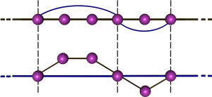
Figure 2: (Color online) A one-dimensional chain of atoms with identical atomic sites each of having on-site potentials $\epsilon$ and hopping integral $t$ with long range hopping $\lambda$ (blue colored line) across $n$-atoms and across $m$-atoms which follow a Fibonacci sequence, as discussed in text. In this particular case we have taken $n=2$ and $m=1$ for instance. The figure below indicates the equivalent decorated version of the buckled ordered chain with restricted long range hopping.

and the hopping integrals are given by,

$$\epsilon_{\alpha} = \epsilon+2t\frac{U_{n-1}(x)}{U_{n}(x)}$$

$$\epsilon_{\beta} = \epsilon+t\left[\frac{U_{n-1}(x)}{U_{n}(x)}+\frac{U_{m-1}(x)}{U_{m}(x)}\right]$$

$$\epsilon_{\gamma} = \epsilon_{\beta}$$

$$t_{L} = \lambda+\frac{t}{U_{n}(x)}$$

$$t_{S} = \lambda+\frac{t}{U_{m}(x)}$$ (3)

Here, $x=(E-\epsilon)/2t$, and $U_{n}(x)$ is the $n$-th order Chebyshev polynomial of the second kind. The resulting effective Fibonacci chain (Fig. 1(b)) is then further renormalized using the standard decimation procedure, viz., by ‘folding’ it backward using the deflation rule $LS\rightarrow L^{\prime}$ and $L\rightarrow S^{\prime}$. The recursion relations relating to the potentials and the hopping matrix elements at one length scale to the next, given by,

$$\epsilon_{\alpha}^{\prime} = \epsilon_{\gamma}+\frac{t_{L}^{2}+t_{S}^{2}}{E-\epsilon_{\beta}}$$

$$\epsilon_{\beta}^{\prime} = \epsilon_{\gamma}+\frac{t_{S}^{2}}{E-\epsilon_{\beta}}$$

$$\epsilon_{\gamma}^{\prime} = \epsilon_{\alpha}+\frac{t_{L}^{2}}{E-\epsilon_{\beta}}$$

$$t_{L}^{\prime} = \frac{t_{L}t_{S}}{E-\epsilon_{\beta}}$$

$$t_{S}^{\prime} = t_{L}$$ (4)

The above equations are exact.

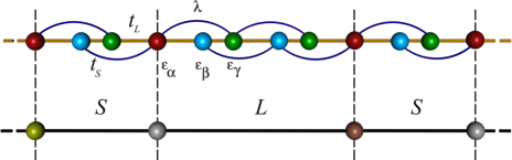
Figure 3: (Color online) Schematic view of a part of an infinite Fibonacci lattice comprising of long ($L$) and short ($S$) bonds having three different kinds of sites $\alpha$ (red sphere), $\beta$ (cyan sphere) and $\gamma$ (green sphere) with corresponding on-site potentials $\epsilon_{\alpha}$, $\epsilon_{\beta}$ and $\epsilon_{\gamma}$ with restricted short ranged $NNN$ interactions shown by blue curved lines. The figure below indicates the renormalized version of the buckled Fibonacci chain.

The spectrum is then easily obtained by calculating the density of states (DOS) by evaluating the Green’s function $G_{\alpha}=(E+i\eta-\epsilon_{\alpha}^{*})^{-1}$ at any local site, say $\alpha$, where, $\epsilon_{\alpha}^{*}$ is the fixed point value of the potential $\epsilon_{\alpha}$, which is achieved when the hopping integrals $t_{L}$ and $t_{S}$ flow to zero under iteration, and $\eta$ is a small imaginary part added to the energy. The DOS is given by, $\rho_{\alpha}=(-1/\pi)\lim_{\eta\rightarrow 0}ImG_{\alpha}(E+i\eta)$.

Before we end this sub-section, it is nice to appreciate that, the “buckling” simulates a long range hopping between sites that are not the nearest neighbors in the parent 1-D chain. The linear lattice depicted in Fig. 1 can be equivalently drawn as a quasiperiodic arrangement of say, squares and triangles (for $n=2$ and $m=1$) where the distant neighbors are connected by an overlap integral $\lambda$. A section of the original linear chain and its quasi-one dimensional equivalent is shown in Fig. 2. Thus the essence of “buckling” is just to bring in the flavor of long range hopping in the system. Interestingly, similar long range hopping is considered recently in a Schrödinger chain, and has been shown to lead to a new extremum at the center of the density of states accompanied by a van Hove singularity  stock .

II.2 Quasiperiodic buckling of a quasiperiodic chain

We consider a Fibonacci chain grown using two letters $L$ and $S$ following the growth rule $L\rightarrow LS$ and $S\rightarrow L$. A segment of an infinite Fibonacci chain is depicted in Fig. 3. The $L$ and $S$ bonds are associated with the hopping integrals $t_{L}$ and $t_{S}$ respectively at the bare scale of length. The three different kinds of sites $\alpha$, $\beta$ and $\gamma$ lie between an $LL$, $LS$ and $SL$ pairs of bonds respectively. We consider buckling of the parent chain such that a tunnel hopping $\lambda$ is established across the combination of $LS$ or $SL$ pairs of bonds, but not across an $LL$ pair. Thus the present model can equivalently be looked at as a quasiperiodic chain with ‘restricted’ second neighbor hopping.

The parent lattice with such restricted second neighbor hopping can be renormalized into a Fibonacci chain with nearest neighbor hoppings only by decimating a subset of vertices and now, using a different length scaling, viz., $LSLSL\rightarrow L^{\prime}$ and $LSL\rightarrow S^{\prime}$.

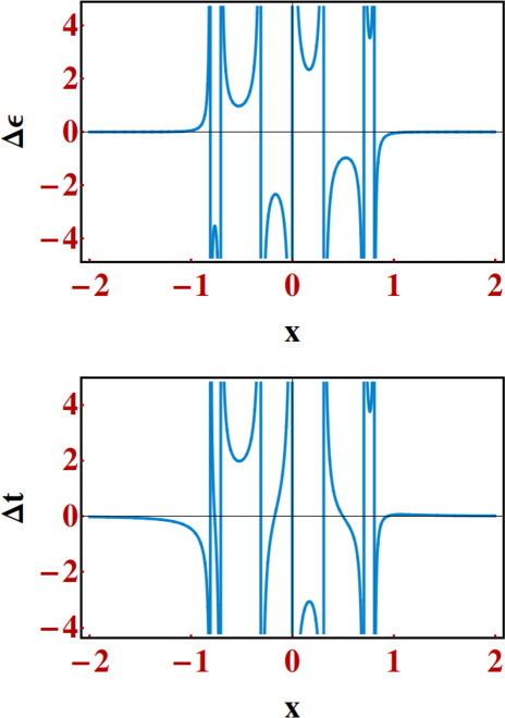
Figure 4: (Color online) (a) $\Delta\epsilon=\epsilon_{\alpha}-\epsilon_{\beta}$ plotted against $x$. We have selected $\epsilon=0$ and $t=1$. $\epsilon_{\alpha}$, $\epsilon_{\beta}$, $t_{L}$ and $t_{S}$ are defined in Eq. (3) and (b) $\Delta t=t_{L}-t_{S}$ plotted against $x$.The dimensionless parameter $x=(E-\epsilon)/2t$ and the energy $E$ is measured in units of $t$.

To evaluate the DOS at any particular site one can use the same set of recursion relations given in Eq. (4).

III Results and discussion

III.1 The periodic chain case

Let us fix, for the sake of clarity, $\epsilon=0$ and $t=1$. Using the set of Eq. (3) we have worked out the difference $\Delta\epsilon=\epsilon_{\alpha}-\epsilon_{\beta}$ and $\Delta t=t_{L}-t_{S}$ with the tunnel hopping being set in the range $-3\leq\lambda\leq 3$. The results are displayed in Fig. 4, as a function of $x=(E-\epsilon)/2t$. It is seen that, for $-4\leq E\leq-2$ and $2\leq E\leq 4$, the differences $\Delta\epsilon$ and $\Delta t$ are both zero, implying that for such ranges of the energy the parameters represent a perfectly ordered chain. Both the graphs show that the system ‘feels’ disorder solely in the energy range $-2\leq E\leq 2$. Due to the specific pattern imposed in the distribution of the buckled segments, this part of the spectrum gets maximally perturbed by the aperiodic distribution of the tunnel hopping $\lambda$. The existence of these localized states are marked by the divergence of $\Delta\epsilon$ at various values of $x$ within the range shown in the figure.

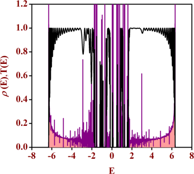
Figure 5: (Color online) Density of states (violet curve) and two terminal electronic transport characteristics (black curve) of an ordered chain buckled sequentially at every $4$-th and $5$-th sites (that is, $n=3$ and $m=4$) following a Fibonacci pattern. We have selected $\epsilon=0$, $t=1$ and $\lambda=3$. Energy is measured in units of the hopping integral $t$. The values of the lead parameters for the transport calculation are $\epsilon_{0}=0$ and $t_{0}=3.5$.

The number of subbands and such localized states depends strongly on the values of $n$, $m$ and of course, on the strength of the tunnel hopping amplitude $\lambda$. But, in every case we come across a scenario where a smooth crossover from an absolutely continuous part in the spectrum to a mixed character, dominated by subbands of narrower widths and point like spectrum, can be engineered.

The DOS, as presented in Fig. 5 exhibits an apparent continuum towards the outer parts of the spectrum with a typical divergence shown by an ordered lattice at the band edges. This can be understood in a perturbative way. For example, when $\lambda$ is large compared to $t$, we can, as a first approximation, ignore $t$ and the system resembles a linear chain with nearest neighbor hopping integral $\lambda$. The band extends from $\epsilon-2\lambda$ to $\epsilon+2\lambda$ and the edges should exhibit a square root divergence as in an ordered chain of atomic sites. If we now ‘switch on’ a non-zero value for $t$, the system starts feeling the presence of a quasiperiodic Fibonacci ordering of the potentials and the nearest neighbor hopping integrals. However, as long as $t$ is not comparable to $\lambda$ only the central part of the spectrum gets affected, while for $t\approx\lambda$, the entire spectrum gets affected, and gap opens everywhere.

As seen in Fig. 5 a gap opens up at the center of the spectrum, punctuated by tiny clusters of isolated peaks. We have extensively investigated the flow pattern in such cases. Typically for any isolated peak in the density of states the number of RSRG iterations vary between $10$ to $15$. This means that the overlap of the Wannier orbitals extends typically over clusters of size $\tau^{10}$ to $\tau^{15}$. Beyond this length the envelope decays down, but this indeed is a slow decay. This scenario is to be contrasted with exponentially localized single particle states (not a member of the continuum regime), for which the hopping integrals flow to zero very quickly (as the wave function of the electron is localized pretty sharply over a limited number of atomic sites) south1 ; south2 . We thus get confidence to comment that such isolated states are critical in the usual sense of a Fibonacci lattice.

On the other hand, the shaded portions of the continuous subbands in the DOS are populated by extended eigenfunctions. For any energy eigenvalue picked up at random from such continuous zones, the nearest neighbor hopping integrals never flow to zero under the RSRG iterations. This proves that the envelopes of the wave functions have non-zero overlap at all scales of length. This means they are extended.

The black curve in Fig. 5 depicts the variation of two-terminal transmission coefficient as a function of the Fermi energy. To calculate the transmission coefficient, we have first placed a large but finite segment of the sample in between two perfectly ordered semi infinite ‘leads’ where the atoms have a constant on-site potential $\epsilon_{0}$ and nearest neighbor hopping integral $t_{0}$. The ordered chain with the quasiperiodic buckling is transformed in to an ‘effective’ Fibonacci chain. The transmission coefficient is then worked out using the well known formula stone , viz.,

$$T(E)=\frac{4\sin^{2}ka}{[(M_{12}-M_{21})+(M_{11}-M_{22})\cos ka)]^{2}+[(M_{11}+M_{22})^{2}\sin^{2}ka]}$$ (5)

where, $\cos ka=(E-\epsilon_{0})/2t_{0}$, $M=M_{R}(\prod M_{i})M_{L}$, with $M_{i}=M_{\alpha}$, $M_{\beta}$ or $M_{\gamma}$ following the Fibonacci sequence generated kohmoto1 , and $M_{R(L)}$ being the transfer matrix corresponding to the atoms sitting at the right and the left extremities respectively. The explicit form of the matrices are,

$$M_{\alpha}=\left(\begin{array}[]{cccc}\frac{(E-\epsilon_{\alpha})}{t_{L}}&-1\\ 1&0\end{array}\right),M_{\beta}=\left(\begin{array}[]{cccc}\frac{(E-\epsilon_{\beta})}{t_{S}}&-\frac{t_{L}}{t_{S}}\\ 1&0\end{array}\right),M_{\gamma}=\left(\begin{array}[]{cccc}\frac{(E-\epsilon_{\gamma})}{t_{L}}&-\frac{t_{S}}{t_{L}}\\ 1&0\end{array}\right)$$ (6)

The ‘left’ and the ‘right’ matrices are also given by,

$$M_{L}=\left(\begin{array}[]{cccc}\frac{(E-\epsilon_{L})}{t_{S}}&-\frac{t_{0}}{t_{S}}\\ 1&0\end{array}\right),M_{R}=\left(\begin{array}[]{cccc}\frac{(E-\epsilon_{R})}{t_{0}}&-\frac{t_{L}}{t_{0}}\\ 1&0\end{array}\right)$$ (7)

Here $\epsilon_{L}$ and $\epsilon_{R}$ are the on-site potentials of the left and right atoms of the finite size atomic chain respectively.

III.2 The Fibonacci chain

We refer to Fig. 3. The infinite Fibonacci chain is buckled so that a tunnel hopping $\lambda$ connects sites separated by an $LS$, or an $SL$ pair, but excludes an $LL$ pair. This geometry equivalently represents a Fibonacci chain with ‘restricted second neighbor hopping’. It is interesting to observe that such a model can be mapped onto a nearest neighbor hopping model by a deflation rule, $LSLSL\rightarrow L^{\prime}$ and $LSL\rightarrow S^{\prime}$. This decimates a subset of sites in the original chain to yield a renormalized version of it. The effective on-site potentials and hopping integrals for this renormalized Fibonacci lattice can be worked out in a tedious, but straightforward manner. For clarity we present below the initial values of the parameters for the effective Fibonacci chain with nearest neighbor interaction. To simplify the cumbersome expressions we select $\epsilon_{\alpha}=\epsilon_{\beta}=\epsilon_{\gamma}=0$ in the original chain. This doesn’t affect the physics as the choice of the on-site potentials only sets the centre of the density of states spectrum. For the ‘new’ Fibonacci chain the parameters read,

$$\epsilon_{\alpha,new}=\frac{{\cal F}_{1}E^{3}+{\cal F}_{2}E^{2}+{\cal F}_{3}E+{\cal F}_{4}}{E^{4}+{\cal G}_{1}E^{2}+{\cal G}_{2}E+{\cal G}_{3}}$$ (8)

$$\epsilon_{\beta,new}=\frac{{\cal F}_{5}E^{5}+{\cal F}_{6}E^{4}+{\cal F}_{7}E^{3}+{\cal F}_{8}E^{2}+{\cal F}_{9}E}{-E^{6}+{\cal G}_{4}E^{4}-{\cal G}_{2}E^{3}+{\cal G}_{5}E^{2}+{\cal G}_{6}E+{\cal G}_{7}}$$

$$\epsilon_{\gamma,new}=\epsilon_{\beta,new}$$

$$t_{L,new}=\frac{{\cal F}_{10}E^{2}+{\cal F}_{11}E+{\cal F}_{12}+{\cal F}_{13}}{E^{4}+{\cal G}_{8}E^{2}+{\cal G}_{2}E+{\cal G}_{9}}$$

$$t_{S,new}=\frac{2\lambda t_{L}E+t_{S}(\lambda^{2}+t_{L}^{2})}{E^{2}-t_{S}^{2}}.$$

where, ${\cal F}_{1}=2(t_{L}^{2}+\lambda^{2})$, ${\cal F}_{2}=4\lambda t_{L}t_{S}$, ${\cal F}_{3}=2[t_{L}^{2}(\lambda^{2}-t_{L}^{2}-t_{S}^{2})-\lambda^{2}(\lambda^{2}+t_{S}^{2})]$, ${\cal F}_{4}=4\lambda t_{L}t_{S}(\lambda^{2}-t_{L}^{2}-t_{S}^{2})$, ${\cal F}_{5}=-2(\lambda^{2}+t_{L}^{2})$, ${\cal F}_{6}=-4t_{L}t_{S}\lambda$, ${\cal F}_{7}=2t_{L}^{4}+4t_{S}^{2}(\lambda^{2}+t_{L}^{2})+\lambda^{2}(2t_{L}^{2}+3\lambda^{2})$, ${\cal F}_{8}=8\lambda t_{L}t_{S}(t_{L}^{2}+t_{S}^{2})+6t_{L}t_{S}\lambda^{3}$, ${\cal F}_{9}=\lambda^{4}(t_{S}^{2}-t_{L}^{2})-\lambda^{6}-t_{L}^{2}t_{S}^{2}(t_{L}^{2}+11\lambda^{2})-2t_{S}^{4}(t_{L}^{2}+\lambda^{2})$, ${\cal F}_{10}=3t_{L}\lambda^{2}$, ${\cal F}_{11}=2\lambda t_{S}(2t_{L}^{2}+\lambda^{2})$, ${\cal F}_{12}=2\lambda^{2}t_{L}(t_{S}^{2}-\lambda^{2})$, ${\cal F}_{13}=t_{L}^{3}(t_{S}^{2}+\lambda^{2})$, ${\cal G}_{1}=-(t_{L}^{2}+2t_{S}^{2}+2\lambda^{2})$, ${\cal G}_{2}=-4\lambda t_{L}t_{S}$, ${\cal G}_{3}=\lambda^{4}-t_{S}^{2}(2\lambda^{2}-t_{S}^{2})$, ${\cal G}_{4}=t_{L}^{2}+3t_{S}^{2}+2\lambda^{2}$, ${\cal G}_{5}=-[\lambda^{4}+t_{S}^{2}(t_{L}^{2}+3t_{S}^{2}+4\lambda^{2})]$, ${\cal G}_{6}=-4\lambda t_{L}t_{S}^{3}$, ${\cal G}_{7}=t_{S}^{6}-\lambda^{2}t_{S}^{2}(\lambda^{2}+2t_{S}^{2})$, ${\cal G}_{8}=-(2t_{S}^{2}+2\lambda^{2}+t_{L}^{2})$, and ${\cal G}_{9}=(t_{S}^{2}-\lambda^{2})^{2}$.

One can now use Eq. (4) with the initial values of the on site potentials and the nearest neighbor hopping integrals as listed above to work out the density of states, as discussed before. The density of states at any site of this renormalized, effectively nearest neighbor Fibonacci chain can be obtained using the recursion relations Eq. (4). The local density of states at an $\alpha$-site is presented in Fig. 6(a), when we introduce the tunnel hopping $\lambda$ at the bare scale of length. This implies that the Fibonacci chain is wrinkled every $LS$ or $SL$ pair. The effect on the spectrum is most severe in this case. However, surprisingly, patches of continuous distribution of eigenvalues turn out to be an interesting feature in this case.

In Fig. 6 we show sequentially the effect of variation of the long range hopping on the density of states. $\lambda$ is chosen to have values $0.5$, $1.0$, $2.0$ and $3.0$ in Fig. 6 (a), (b), (c) and (d) respectively. While for $\lambda=0.5$ the density of states does not show any significant continuum, for $\lambda=1.0$, a trace of a continumm appears to the left of $E=0$. The continuum appears much more prominently as $\lambda$ increases to $2.0$ and $3.0$ respectively. For each such case, we have tested the flow of the hopping integrals under successive renormalization. The hopping integrals, for any energy eigenvalue picked at random from such dense patches of energy, keep on oscillating without converging to zero, indicating that the states are extended in character. We have thoroughly examined such regimes with finer and finer scanning of the intervals of energy.

In Fig. 7 we impart buckling on a $20$ times

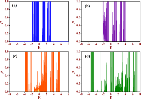
Figure 6: (Color online) Density of states of an infinite Fibonacci chain as a function of the energy for different combination of buckling constant $\lambda$. The buckling has been applied at the bare length scale. We have set $\epsilon_{i}=0$, $i=\alpha$, $\beta$ and $\gamma$. $t_{L}=1$, $t_{S}=1.5$. Energy is measured in units of $t_{L}$. The values of the buckling parameters in the following four cases respectively are (a) $\lambda=0.5$ (b) $\lambda=1.0$ (c) $\lambda=2.0$ (d) $\lambda=3.0$.

renormalized Fibonacci chain to begin with. Naturally, such a long chain retains the essential features of an infinite lattice. The figure shows the three subband structure in the DOS pattern, a trademark of the transfer model of a Fibonacci chain kohmoto2 . However, the bound states caused by the buckling are still observed within the spectral gaps of the three subband area, as well as outside the global band edges.

The fine structure of the spectrum is brought out as shown in Fig. 7(b) around the central part. The typical self similar three subband spectrum opens up, with further splitting being visible. The additional feature is the appearance of sharply localized bound states inside the multiple gaps in the spectrum, indicating a self similar distribution of the bound states as well.

The two terminal transport across a $144$-bond long Fibonacci chain, buckled at the bare length scale with the strength of the tunnel hopping $\lambda$ following the sequence of values as in Fig.6, is shown in Fig. 8. The parameters are the same as those in Fig. 6. The absolutely continuous character present in the density of states spectrum is corroborated by a continuous zone of

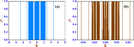
Figure 7: (Color online) Density of states of an infinite Fibonacci chain. (a) Buckling is applied to a $20$ times renormalized Fibonacci chain. (b) Enlarged central part of (a) to bring out the inherent self similarity displayed by the distribution of the eigenvalues. We have set $\epsilon_{i}=0$, $i=\alpha$, $\beta$ and $\gamma$. $t_{L}=1$, $t_{S}=1.5$ and $\lambda=2.5$. Energy is measured in units of $t_{L}$.

high transmission coefficient which certify for the extended character of the spectrum.

To end, we find it instructive to illustrate the distribution of the energy eigenvalues

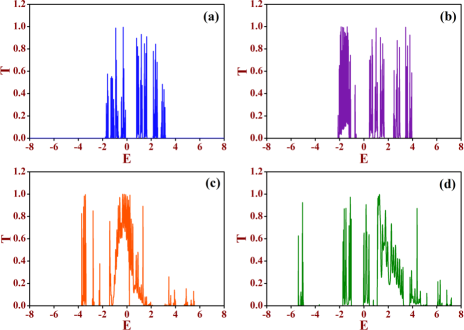
Figure 8: (Color online) Two-terminal transmission characteristics of a Fibonacci chain with $144$ bonds as a function of the energy for different combination of buckling constant $\lambda$. The buckling has been applied at the bare length scale. We have set $\epsilon_{i}=0$, $i=\alpha$, $\beta$ and $\gamma$. $t_{L}=1$, $t_{S}=1.5$. Energy is measured in units of $t_{L}$. The values of the buckling parameters in the following four cases respectively are (a) $\lambda=0.5$ (b) $\lambda=1.0$ (c) $\lambda=2.0$ (d) $\lambda=3.0$.

of a buckled Fibonacci chain as a function of the tunnel hopping amplitude $\lambda$. Fig. 9 displays the effect of buckling. The four panels correspond to

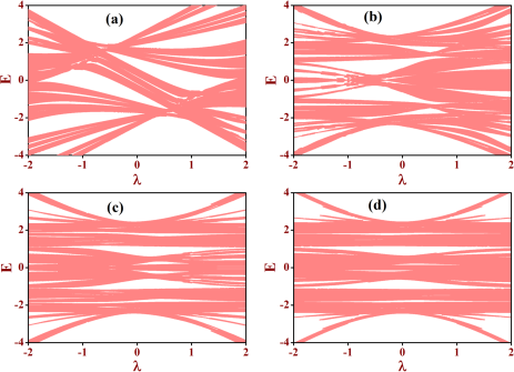
Figure 9: (Color online) $E$ versus $\lambda$ profile of a Fibonacci lattice at different stage of initial renormalization (a) $n=0$, (b) $n=2$, (c) $n=4$ and (d) $n=6$. The parameters are $\epsilon_{\alpha}=\epsilon_{\beta}=\epsilon_{\gamma}=0$ and $t_{L}=1$ and $t_{S}=1.5$.

the different scales of length at which the buckling has been introduced. Panel (a) shows the effect when the chain is bent at its bare scale of length.

In general, the energy spectrum of a Fibonacci quasicrystal, in an off-diagonal model, consists of three fragmented subbands, each splitting further into three self similar subbands on finer scan over the energy interval kohmoto1 . In the present case, with buckling at the bare scale of length we can see that this three subband pattern is destroyed. The effect of the buckling is maximum here. The bound states arising out of the sequential bending are not visible prominently, but the global three subband spectral splitting of a Fibonacci chain with nearest neighbor interaction is lost. With the buckling introduced over longer segments, achieved by renormalizing the original chain, say, two, four or six times first, the three subband pattern seems to be getting restored gradually, and is quite apparent in the last of the panels, that is, (d). This is understandable, as the introduction of the buckling through a longer range tunnel hopping on an $n$-step renormalized lattice implies that the nearest neighbor quasiperiodic chain’s spectrum is preserved as we have larger and larger segments of ‘clean’ Fibonacci lattice trapped in the bent zone for increasing values of $n$. The appearance of the bound states are also apparent as $\lambda$ increases.

IV conclusion

We have addressed the problem of the changes brought about in the electronic spectra of a perfectly periodic chain of atoms and in a quasiperiodic Fibonacci chain when finite segments of them are buckled to bring two distant neighbors into close proximity. This ‘proximity’ is modeled by a tunnel hopping connecting these distant neighbors. We have used a real space renormalization group decimation scheme to map the chains with restricted long range hoppings on to chains with renormalized on-site potentials and nearest neighbor hopping integrals, both being functions of the energy of the electron. It is seen that the buckling induced spectral characters of the pure and the quasiperiodic chain are quite contrasting. With large values of the tunnel hopping integral, a measure of the amount of buckling, the ‘ordered’ chain can retain its absolutely continuous part towards the end of the spectrum, populated by extended eigenstates only, while the central part turns ‘dirty’ and offers a mixed character of extended and localized states. This can be utilized to look for a possible ‘switch on’, ‘switch off’ effect in its electronic conduction.

The Fibonacci chain on the other hand, shows the startling appearance of one or more absolutely continuous subbands populated by unscattered (extended) eigenstates flanked by the usual critical ones. The appearance of sharply localized, bound states mark both the case, particularly when the buckling is large, that is the tunnel hopping integral $\lambda$ assumes a large value compared to the intrinsic hopping parameters of the systems. Such states appear to get distributed in a self similar manner, a fact that becomes more apparent when the buckling is introduced over larger and lager segments of the original Fibonacci chain.

It is to be appreciated that the long range hopping brings in a flavour of the formation of rings, providing additional path for the electron to jump to a distant site. The ‘buckling’ essentially gives rise to the formation of polygonal structures (see Fig. 2). For example, with $n=2$ and $m=1$ one encounters a sequence of trapezia and triangles, the latter creating frustration and the anti-bonding states gets pushed away in energy. This has immense effect on the localization properties  naumis2 . Such buckling has been implemented experimentally in graphene nanoribbons very recently lit for both in-plane and out-of-plane bendings, and the changes in the density of states have been probed. The spectrum is not unlikely to display similar or even richer properties if one studies a two dimensional strip, buckled and stressed. This will be addressed theoretically in a future communication.

- (1) P. W. Anderson, Phys. Rev. 109, 1492 (1958).
- (2) B. Kramer and A. MacKinnon, Rep. Prog. Phys. 56, 1469 (1993).
- (3) E. Abrahams, P. W. Anderson, D. C. Licciardello, and T. V. Ramakrishnan, Phys. Rev. Lett. 42, 673 (1979).
- (4) R. A. Römer and H. Schulz-Baldes, Europhys. Lett. 68, 247 (2004).
- (5) A. Eilmes, R. A. Römer, and M. Schreiber, Physica B 296, 46 (2001).
- (6) A. Rodríguez, J. Phys. A: Math. Gen. 39, 14303 (2006).
- (7) S. D. Pinski, W. Schirmacher, and R. A. Römer, Europhys. Lett. 97, 16007 (2012).
- (8) Lev I. Deych, A. A. Lisyanski, and B. L. Altshuler, Phys. Rev. Lett. 84, 2678 (2000).
- (9) J. W. Kantelhardt and A. Bunde, Phys. Rev. B 66, 035118 (2002).
- (10) M. Titov and H. Schomerus, Phys. Rev. Lett. 95, 126602 (2005).
- (11) M. Kohmoto, B. Sutherland, and C. Tang, Phys. Rev. B 35, 1020 (1987).
- (12) M. Kohmoto and J. Banavar, Phys. Rev. B 34, 563 (1986).
- (13) Nicolas Macé, Anuradha Jagannathan, and Frédéric Piéchon, Phys. Rev. B 93, 205153 (2016).
- (14) B. Sutherland and M. Kohmoto, Phys. Rev. B 36, 5877 (1987).
- (15) S. Das Sarma and X. Xie, Phys. Rev. B 37, 1097 (1988).
- (16) E. Macia and F. Dominguez-Adame, Phys. Rev. Lett. 76, 2957 (1996).
- (17) V. K. Verma, S. Pilati, and V. E. Kravtsov, Phys. Rev. B 94, 214204 (2016).
- (18) P. R.- Taboada and G. G. Naumis, Phys. Rev. B 92, 035406 (2015).
- (19) K. Vacek, H. Kasai, and A. Okiji, J. Phys. Soc. of Japan, 61, 27 (1992).
- (20) O. O. Vakhnenko, Phys. Lett. A 211, 46 (1996).
- (21) S.-J. Xiong and S. N. Evangelou, Phys. Rev. B 52, R13079(R) (1995).
- (22) S.-J. Xiong, Y. Chen, and S. N. Evangelou, Phys. Rev. Lett. 77 4414 (1996).
- (23) F. Guinea and J. A. Vergés, Phys. Rev. B 35, 979 (1987).
- (24) F. Zhong, L. Zuli, Y. Kailun, and H. U. Huifang, Commun. Theor. Phys. 28, 29 (1997).
- (25) J. Stockhofe and P. Schmelcher, Phys. Rev. A 92, 023605 (2015).
- (26) B. W. Southern, A. A. Kumar, and J. A. Ashraff, Phys. Rev. B 28, 1785 (1983).
- (27) B. W. Southern, A. A. Kumar, P. D. Loly, and A.-M.S. Tremblay, Phys. Rev. B 27, 1485(R) (1983).
- (28) A. D. Stone, J. D. Joannopoulos, and D. J. Chadi, Phys. Rev. B 24, 5583 (1981).
- (29) J. E. Barrios-Vargas and G. G. Naumis, J. Phys. Condens. Mat. 23, 375501 (2011).
- (30) J. van der Lit, P. H. Jacobse, D. Vanmaekelbergh, and I. Swart, New. J. Phys. 17, 053013 (2015).