Spin breather and rogue formations in a Heisenberg ferromagnetic system

Abstract

We construct explicit spin configurations for the breather solution of a one-dimensional Heisenberg ferromagnetic spin system. This corresponds to the breather soliton solution of the gauge equivalent nonlinear Schrödinger equation. There are three broad cases, wherein the solution shows distinct behavior. Of particular interest to our study is the rogue behavior in spin field terms.

1 Introduction

The Heisenberg model of spin interaction has been a subject of keen interest for decades. Although fundamentally quantum in nature, for low level excitations its classical counterpart has nevertheless yielded important physically realizable results. The bare Heisenberg model in one-dimension (1-d) is perhaps the simplest yet non-trivial nonlinear model among the larger class of O(3) sigma modelsrr:1987 ; zakr:1989 . The 1-d model is completely integrable with soliton solutions, and is gauge equivalent to the nonlinear Schrödinger equation (NLSE)ml:1977 ; takt:1977 ; zs:1972 . The classical model in 2-d, though not known to be integrable, has a very interesting class of solutions called skyrmions that fall into distinct topological sectors identified by the Hopf invariantbp:1975 .

The NLSE is another fundamental model naturally and frequently arising in a variety of physical systems such as fluid dynamics, dynamics of polymeric fluids, fiber optics and vortex dynamics in superfluids, to name a few hb:1982 ; hasi:1972 ; bird:1987 ; hase:1989 ; schw:1988 . Besides its physical importance, it also is a very important model in soliton theory, owing to its rich mathematical structure. It is completely integrable with soliton solutions, and presents itself amenable to nearly every method available in the study of nonlinear systems, making it a perfect pedagogical model. Its complete integrability was first established in a classic paper by Zakharov and Shabat in 1972, which also brought about a deeper clarity, from a geometric point of view, on the method of inverse scattering transform being developed around that periodzs:1972 ; sulem:1999 . For this reason it remains one of the most studied, and among the most understood of nonlinear systems. Besides NLSE, further extensions of the system, such as the N-coupled NLSE, multidimensional NLSE, higher order NLSE, to name a few, have often proved fruitful in studying several physical systems of importance. Inspite of its rich history and continued interest, investigations on NLSE have often thrown out novel results and physical behavior never anticipated or intuited earlier. One such is the rogue wave solutions, marked by a sudden, momentary yet colossal enhancement in the field variablema:1979 ; pere:1983 ; akhm:1986 . Interest in this special solution have grown manifold since citing of similar phenomenon in the deep oceankharif:2008 . Besides, the same have been predicted to occur in Bose-Einstein condensates, whose dynamics is modeled by the Gross-Pitaevskii equation, which closely resembles the NLSE in higher dimensionakhm:2009 .

In this paper, we exploit this gauge equivalence between the Heisenberg ferromagnet and NLSE to study and illustrate the equivalent rogue behavior in an 1-d spin field. Furthermore, a natural connection exists between the spin field in 1-d and a space curve in 3-d, its dynamic evolution spanning a surface. In the case of systems integrable and endowed with a Lax pair the soliton surfaces thus obtained are of much interest geometrically in soliton theorysym:1985 . Often the space curves thus obtained are by themselves physically realizable, adding to their significancesm:2005 . Here, however, we shall restrict ourselves to obtaining the breather spin field for the Heisenberg spin chain, especially demonstrating the rogue behavior. In the next section, we introduce the model briefly and, after an outline of the method of obtaining the solution, give the general expression for the breather spin field. We also discuss in detail two cases, determined by the relative values of the relevant parameters, wherein the behavior of the breather modes are pronouncedly distinct. The rogue phenomenon is illustrated as a special limiting case of these two behaviors.

2 The rogue spin field

The classical Heisenberg ferromagnet (HF) is governed by the hamiltonian

$$\mathbf{H}=J\int{\nabla{\bf\hat{S}}}^{2}$$ (1)

where $J$ is a constant arising out of the exchange integral, positive for a ferromagnet, and ${\bf\hat{S}}(x,t)=\{S_{1},S_{2},S_{3}\}$ is the unit spin field ($|{\bf\hat{S}}|=1$) of interest. In this paper, we shall be concerned only with the 1-d spin chain. Using the spin commutation relations one gets the simplest form of the Landau-Lifshitz equation (LLE) governing its dynamics (after rescaling $t$)

$${\bf\hat{S}}_{t}=-{\bf\hat{S}}\times{\bf\hat{S}}_{xx},$$ (2)

where the subscripts stand for partial derivatives, as usual. As mentioned earlier, the 1-D LLE, Eq. (2), is integrable through inverse scattering method with soliton solutions, and can be expressed through the auxiliary linear equationsfad:1987

$$\Phi_{x}=U_{HF}\Phi=\frac{-i\lambda}{2}{\bf S}\Phi$$

$$\Phi_{t}=V_{HF}\Phi=\Big{(}\frac{\lambda}{2}{\bf S}_{x}{\bf S}+\frac{i\lambda^{2}}{2}{\bf S}\Big{)}\Phi.$$ (3)

Here

$${\bf S}=S_{i}\sigma_{i},$$ (4)

(summation assumed) with $\sigma_{i},\,\,i=1,2,3$ being the Pauli matrices, and $S_{i}$ the components of the unit spin field ${\bf\hat{S}}$, and $\lambda$ is the scattering parameter. Thus, $U_{HF}$ and $V_{HF}$ form the Lax pair for the system. The compatibility of the two equations, Eq. (2), gives the matrix form of the LLE:

$${\bf S}_{t}=\frac{-i}{2}[{\bf S},{\bf S}_{xx}],$$ (5)

which, when expressed in scalar form, gives back Eq. (2).

The most prominent solution of the Heisenberg model in 1-d is the localized traveling wave solution of the ‘secant-hyperbolic’ variety, associated with the isolated soliton solution of the NLSE. The NLSE

$$i\psi_{t}+\psi_{xx}+2|\psi|^{2}\psi=0$$ (6)

supports the trivial solution $\psi=0$. Taking this as a seed solution, any of the standard methods of obtaining soliton solutions would yield a one-soliton solution of the form

$$\psi=\lambda_{0I}{\rm sech}\omega_{0I}e^{i\omega_{0R}},$$ (7)

where $\omega_{0}=\omega_{0R}+i\omega_{0I}=\lambda_{0}x-\lambda_{0}^{2}t-(\varphi_{1}+i\varphi_{2})$, and $\lambda_{0}=\lambda_{0R}+i\lambda_{0I}$ is the complex eigenvalue on the plane of the scattering parameter that determines the amplitude and velocity of the soliton. $\varphi_{1,2}$ are arbitrary constants indicating the initial phase and position of the soliton. Of particular interest to us for the following discussion, as we shall see below, is when $\lambda_{0}$ is purely imaginary, in which case the soliton is stationary, localized spatially and temporally periodic.

The NLSE also permits a temporal wave solution of the form

$$\psi_{0}(x,t)=Ae^{2iA^{2}t},$$ (8)

where $A$ is some positive real constant. While the isolated soliton corresponds to a vanishing boundary condition at infinity, this seed form, Eq. (8), leads to a solution that decays to a uniform solution. Starting with this seed solution (or equivalently, a spatially static wave solution of the form $\psi_{0}=ke^{\pm i\frac{k}{\sqrt{2}}x}$, $k$ being any real constant, or a plane traveling wave with a suitable dispersion relation, obtained through an appropriate gauge transformation to $\psi(x,t)$), one may still go ahead to find a more non-trivial solution through any of the standard inverse scattering transform methods. Such a solution, the breather, has indeed been obtained by a host of authorsma:1979 ; pere:1983 ; akhm:1986 . The general form of the solution is given by

$$\psi_{r}=e^{2iA^{2}t}\Bigg{[}A\,+\,2\,\lambda_{0I}\,\frac{\big{(}\zeta-i\,\eta\big{)}}{Z}\,\Bigg{]}$$ (9)

where $\lambda_{0}$ is the complex eigenvalue, as remarked earlier, associated with the one-soliton solution, and $A$ is the amplitude in Eq. (8).
$Z=-2\,A\,\Im(\mu)\,\cos(2\,\Re(\Omega_{0}))+\alpha\,\cosh(2\,\Im(\Omega_{0})+2K)$
$\zeta=\alpha\,\cos(2\,\Re(\Omega_{0}))-2\,A\,\Im(\mu)\,\cosh(2\,\Im(\Omega_{0})+2K)$
$\eta=-\beta\,\sin(2\,\Re(\Omega_{0}))+2\,A\,\Re(\mu)\,\sinh(2\,\Im(\Omega_{0})+2K)$
$\Omega_{0}=2\,t\,p_{0}\,\lambda_{0}\,+p_{0}\,x\,-\phi_{0}$
$p_{0}^{2}=A^{2}+{\lambda_{0}}^{2}$.
$\mu=(\lambda_{0}-p_{0})$
$\alpha=2\,\Big{(}\lambda_{0I}^{2}+\Re(p_{0})^{2}-\lambda_{0R}\,\Re(p_{0})-\lambda_{0I}\,\Im(p_{0})\Big{)}$
$\beta=2\,\Big{(}\Im(p_{0})^{2}+\lambda_{0R}^{2}-\lambda_{0R}\,\Re(p_{0})-\lambda_{0I}\,\Im(p_{0})\Big{)}$
For special values of $A$ and $\lambda_{0}$, it displays a rogue behavior, marked by sudden, short, yet colossal rise in the field magnitude.

Here we present its spin analogue - the rogue spin wave. To do so, we briefly outline the procedure to be followed using the gauge equivalence of the 1-d Heisenberg model and the NLSE takt:1977 ; fad:1987 ; schief:2002 . It may be noted that the spin field ${\bf S}$, as expressed in Eq. (4), and the Lax pair in Eq. (2) are elements of the $su(2)$ lie algebra. Consequently, the auxiliary function $\Phi$ lives in the $SU(2)$ group. The auxiliary equations associated with the NLSE similarly indicate that the Lax pair for NLSE are elements of $su(2)$, with auxiliary functions in the $SU(2)$ group. If we denote these auxiliary functions by $\Phi_{NLS}$ then the spin field ${\bf S}$, Eq. (4), and the equivalent LLE, Eq. (2), can be obtained through a unitary transformation

$${\bf S}=\lim_{\lambda\to 0}\Phi_{NLS}^{\dagger}\sigma_{3}\Phi_{NLS}^{~{}}.$$ (10)

Finally, one writes the corresponding vector field ${\bf\hat{S}}$ making use of the isomorphism between $su(2)$ lie algebra and the euclidean $\mathbf{R}^{3}$. The energy densities in the two descriptions are related as

$$\mathbf{E}=\frac{1}{2}{\bf\hat{S}}_{x}^{2}=|\psi|^{2},$$ (11)

and the momentum density of the spin field is given bytjon:1977

$$\mathbf{p}_{x}=\frac{\partial\phi}{\partial x}(1-S_{3}),$$ (12)

where $\phi=\tan^{-1}(S_{2}/S_{1})$.

Going by this procedure, the spin field corresponding to the seed solution Eq. (8) is derived to be

$${\bf\hat{S}}_{0}=\tanh(2K)\sin(2px-2\phi_{0}){\bf\hat{i}}+\cos(2px-2\phi_{0}){\bf\hat{j}}$$

$$+{\rm sech}(2K)\sin(2px-2\phi_{0}){\bf\hat{k}},$$ (13)

where $p=|A|$, and $K$ and $\phi_{0}$ are arbitrary constants, arising out of the translational invariance and global rotation symmetry of LLE, respectively. It may be noted that this seed spin field is independent of $t$, but depends on $x$ (although $\psi_{0}$ is not), and provides a simple yet non-trivial static solution for LLE, Eq. (2). Besides, it is periodic in $x$. These two observations aren’t surprising. For, as indicated earlier, it merely amounts to a suitable gauge transformation to the NLSE seed solution $\psi_{0}(x,t)$, Eq. (8).

Continuing with this procedure to find the one-soliton solution, after some straight forward but tedious calculation, the rogue spin wave is found to be of the form:

$${\bf\hat{S}}_{1}=\frac{p}{A|\lambda_{0}|^{2}}\big{(}\lambda_{0R}^{2}-\lambda_{0I}^{2}\big{)}{\bf\hat{S}}_{0}+\Big{[}-\frac{2\,\lambda_{0I}^{2}}{A\,Z^{2}|\lambda_{0}|^{2}}\Pi\xi$$

$$+\frac{2}{A\,Z|\lambda_{0}|^{2}}\,\lambda_{0I}\,\lambda_{0R}\,\Big{(}A\,\tanh(2K)\,\cos(2px-2\phi_{0})\,\eta$$

$$-p\,{\rm sech}(2K)\,\zeta\Big{)}\Big{]}{\bf\hat{x}}$$

$$+\Big{[}\frac{2\,\lambda_{0I}^{2}}{A\,Z^{2}|\lambda_{0}|^{2}}\,\Delta\,\xi-\frac{2}{Z|\lambda_{0}|^{2}}\,\lambda_{0I}\,\lambda_{0R}\,\sin(2px-2\phi_{0})\,\eta\Big{]}{\bf\hat{y}}$$

$$+\Big{[}\frac{2\,\lambda_{0I}^{2}}{A\,Z^{2}|\lambda_{0}|^{2}}\ \Gamma\,\xi$$

$$-\frac{2}{A\,Z|\lambda_{0}|^{2}}\,\lambda_{0I}\,\lambda_{0R}\,\Big{(}A\,{\rm sech}(2K)\,\cos(2px-2\phi_{0})\,\eta$$

$$+p\,\tanh(2K)\,\zeta\Big{)}\Big{]}{\bf\hat{z}},~{}~{}~{}~{}~{}~{}$$ (14)

where, besides the parameters defined below Eq. (9),
$\Gamma=A\,{\rm sech}(2K)\,\cos(2px-2\phi_{0})\,\zeta-p\,\tanh(2K)\,\eta\\ ~{}~{}~{}~{}~{}+p\,{\rm sech}(2K)\,\sin(2px-2\phi_{0})\,\xi$
$\Pi=-p\,\tanh(2K)\,\sin(2px-2\phi_{0})\,\xi\\ ~{}~{}~{}~{}~{}-A\,\tanh(2K)\,\cos(2px-2\phi_{0})\,\zeta-p\,{\rm sech}(2K)\,\eta$
$\Delta=p\,\cos(2px-2\phi_{0})\,\xi-A\,\sin(2px-2\phi_{0})\,\zeta$
$\xi=-2\,A\,\Re(\mu)\,\sin(2\,\Re(\Omega_{0}))-\beta\,\sinh(2\,\Im(\Omega_{0})+2K)$
The form and behavior of spin field is dictated by two parameters — the amplitude $A$, and $\lambda_{0}$ the complex eigenvalue on the plane of the scattering parameter associated with the one soliton. The relative values of the two parameters lead to broadly three characteristic behavior in the spin field. However, as is clear from the form of the solution Eq. (2), it is cumbersome to analyze the behavior in its entire generality. For our further analysis, therefore, we shall consider only the special case $A>0$, and that the eigenvalue is purely imaginary, $\lambda_{0}=ia$, where $a$ is positive (It may be recalled that for the NLSE the eigenvalues can assume values only on the upper half of the complex plane of the scattering parameterspn:1984 ). The spin field in Eq. (2) then takes a simpler form

$${\bf\hat{S}}_{1}=-\frac{2\xi}{A\,Z^{2}}\Big{[}\Pi{\bf\hat{x}}-\Delta\,{\bf\hat{y}}-\Gamma\,{\bf\hat{z}}\Big{]}-{\bf\hat{S}}_{0}.$$ (15)

There are three distinct cases i) $A<a$, ii) $A>a$ iii) $A=a$. However, the last case is trivial, reducing to the background field due to the seed. The more interesting situation is $A\sim a$ which leads to a rogue behavior. We discuss these three situations in detail below:

2.1 Case i: $A<a$

Firstly, it is verified that as $A\to 0$, the form of the rogue soliton, Eq. (9), approaches the isolated one-soliton, Eq. (7), as expected. An illustrative plot of the energy and momentum densities for $A(\neq 0)<a$, are plotted in Fig. 1. The spin field is localized in space, but shows an oscillatory behavior in time, with a period

$$T=\frac{\pi}{2a\sqrt{a^{2}-A^{2}}}.$$ (16)

As remarked earlier, this behavior is that of the isolated one-soliton for purely imaginary $\lambda_{0}$. The form of the spin field itself is shown in Fig. 2.a.

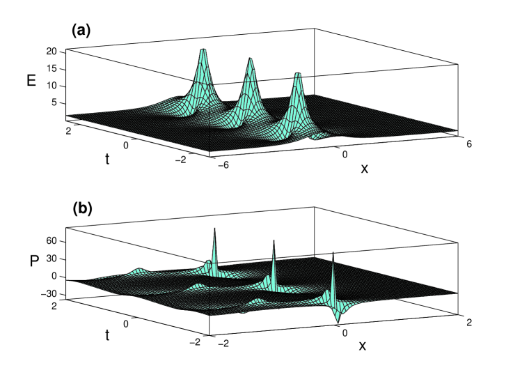
Figure 1: The energy (a) and momentum (b) densities for the temporally periodic, and spatially localized, spin field in the $x-t$ plane for $A<a$ — Kuznetsov-Ma breather. Qualitatively, this is similar to the one-soliton spin field for the 1-D HF model, except that it is non-traveling, due to the eigenvalue $\lambda_{0}$ being purely imaginary.

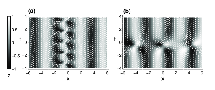
Figure 2: The spin fields (2-d projections) for the two cases i. $A<a$ — Kuznetsov-Ma breather (a) and ii. $A>a$ — Akhmediev breather (b). Grey scale indicates the strength of the $z$-component, $S_{z}$.

2.2 Case ii: $A>a$

At $A=a$, the spin field is reduced to the background seed field that we started with. However, as the magnitude of $A$ makes the cross over from $A<a$ to $A>a$, we see an interesting change in the form of the associated spin field. The temporal periodicity witnessed earlier is replaced by a spatial periodicity, while more interestingly, the field is now temporally local. Spatially, the field is composed of two periodic functions with periods

$$L_{1}=\frac{\pi}{A},\,\,{\rm and}\,\,L_{2}=\frac{\pi}{\sqrt{A^{2}-a^{2}}},$$ (17)

which are in general non-commensurate. Neither of the two field configurations presented here possess a traveling nature owing to the fact that we have chosen $\lambda_{0}$ to be purely imaginary for the sake of ease in analysis. A more general complex $\lambda_{0}$, while retaining the overall general property, renders the filed a traveling nature with uniform speed determined by $\lambda_{0}$, as is expected of a soliton. The energy and momentum densities are shown in Fig. 3, while the field configuration is shown in Fig. 2.b.

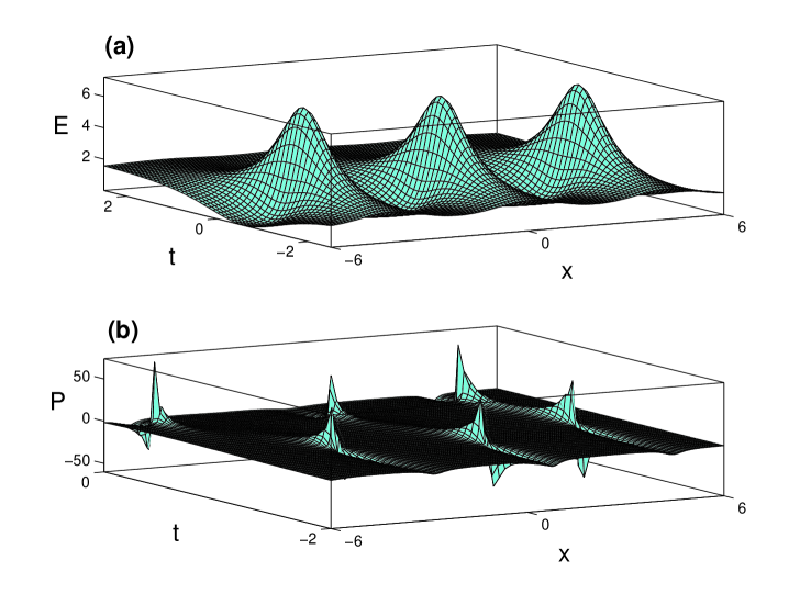
Figure 3: The energy density $\mathbf{E}$ (a) and the momentum $\mathbf{P}$ (b) fields in the $x-t$ plane for $A>a$ — Akhmediev breather. The periodicity in time, seen in case i, is replaced by a spatial periodicity. Temporally the excitations are localized.

2.3 Case iii: $|A-a|=\epsilon\sim 0$ — the rogue field

We do not discuss the case $A=a$ in detail, as, in that case the spin field is reduced to the seed field, Eq. (2), i.e, the background field. The field is time independent, periodic in space and has a uniform energy density.

However, $|A-a|\sim 0$ is a case of special interest, as it is in this regime that the spin field shows the rogue behavior. This can be understood from the expression for temporal period, Eq. (16), when $A<a$, and similarly from Eq. (17) for the spatial period when $A>a$. Although we have already noticed glimpses of periodic rogue behavior in cases i and ii, the phenomenon is more pronounced as $|A-a|\to 0$, since both the periods $T\,,L_{2}\,\to\infty$ (see Eqs. (16 and 17, respectively). Especially, when $A>a$, a sudden localized colossal raise in magnitude of the field is witnessed, as seen in the plot of the energy density in Fig. 4.

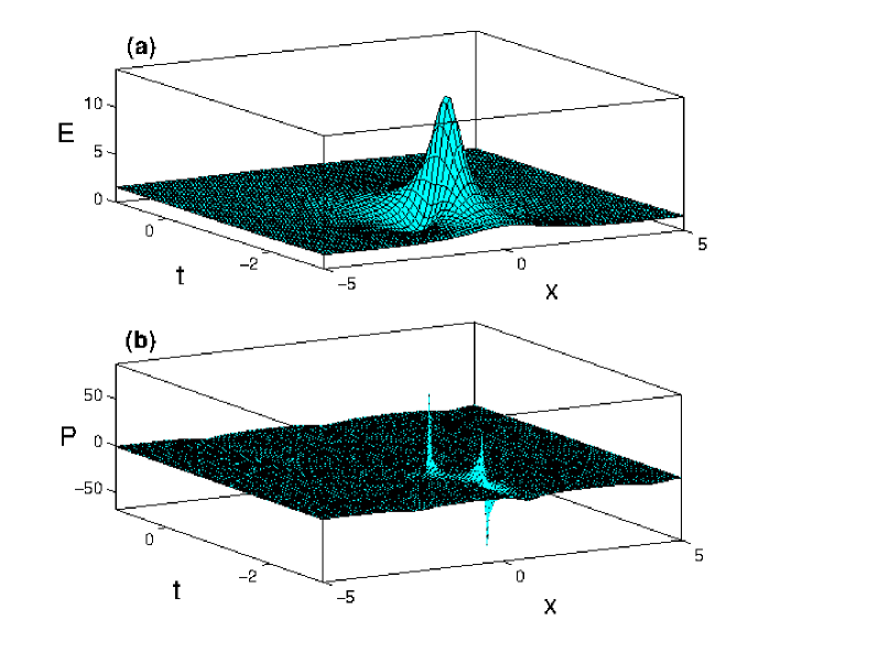
Figure 4: The energy density $\mathbf{E}$ (a) and the momentum $\mathbf{P}$ (b) fields in the $x-t$ plane for $A\sim a$ — Peregrine breather. The spatial period widens to present a colossal excitation localized in space and time.

A profile of the spin field itself for the narrow region in space time when the rogue behavior is witnessed is shown in Fig. 5. An animation of the rogue behavior of the spin field in illustrated in movie1.

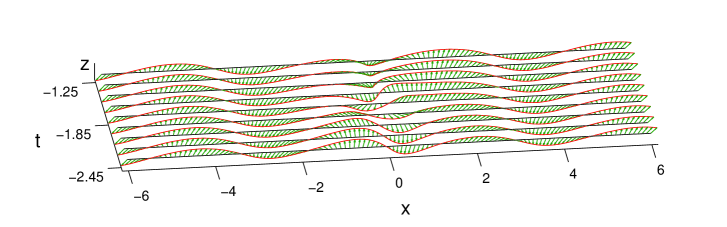
Figure 5: The profile of the spin field in the narrow $x-t$ region of rogue behavior.

3 Conclusion

We have studied the breather spin configuration for 1-D Heisenberg ferromagnet, whose dynamics is governed by the integrable Landau-Lifshitz equation. The expression for the breather field is explicitly obtained, and three distinct cases, based on relative parameter values studied. Particularly, for a special choice of parameters, the breather shows a rogue behavior marked by a colossal field excitation, yet local in space in time. As indicated in Section 2, the breather solutions correspond to a special periodic boundary condition, which we believe is possible to obtain experimentally, leading to the possibility of achieving a rogue spin field in the laboratory. The primary interest in solitons is due to their characteristic properties — localized, shape preserving, traveling and robust under collision. Of these, robustness under collisions has what has made them an attractive proposition application wise. Solitons owe this property to the integrable nature of the dynamical equation, and for this reason the same character must be carried over by rogue solitons as well under collision. Nevertheless, a direct confirmation on this aspect would open prospects of several applications based on the rogue behavior. In the near future, we intend to carry a detailed study on their collision behavior.

References

- (1) R. Rajaraman, Solitons and Instantons (North Holland Amsterdam, 1987).
- (2) W. J. Zakrzewski, Low Dimensional Sigma Models (CRC Press, 1989).
- (3) M. Lakshmanan, Phys. Lett. A. 61, (1977) 53-54.
- (4) Takhtajan, L. A. Phys. Lett. A. 64, (1977) 235-237.
- (5) V. E. Zakharov and A. B. Shabat, Soviet Phys. JETP 34, (1972) 62-69.
- (6) A. Belavin and A. M. Polyakov, JETP Lett. 22, (1975) 245-247.
- (7) E. J. Hopfinger and F. K. Browand, Nature 295, (1982) 393-395.
- (8) H. Hasimoto, J. Fluid Mech. 51, (1972) 477-485.
- (9) R. B. Bird, R. C. Armstrong and O. Hassager, Dynamics of Polymeric Liquids, Volume 1 (Wiley-Blackwell, 1987).
- (10) A. Hasegawa, Optical Solitons in Fibers (Springer-Verlag Berlin, 1989).
- (11) K. W. Schwarz, Phys. Rev. B 38, (1988) 2398-2417.
- (12) Sulem C and Sulem P L, The Nonlinear Schrödinger equation - Self-focusing and wave collapse (Springer-Verlag New York, 1999).
- (13) Yan-Chow Ma, Stud. Appl. Math. 60, (1979) 43-58.
- (14) D. H. Peregrine, J. Austral. Math. Soc. Ser. B 25, (1983) 16-43.
- (15) N. N. Akhmediev and V. I. Korneev, Theor. Math. Phys. 69, 1986 1089-1093.
- (16) C. Kharif, E. Pelinovsky and A. Slunyaev, Rogue Waves in the Ocean (Springer Berlin, 2008).
- (17) Yu. V. Bludov, V. V. Konotop and N. Akhmediev, Phys. Rev. A 80, (2009) 033610.
- (18) A. Sym, in Geometric Aspects of the Einstein Equations and Integrable Systems, edited by R. Martini (Springer Berlin 1985), pp. 154-231.
- (19) S. Murugesh and M. Lakshmanan, Int. J. Bif. Chaos 15, (2005) 51-63.
- (20) Aritra K. Mukhopadhyay, Vivek M. Vyas and Prasantha K. Panigrahi, Euro. Phys. Jour. B. 88, (2015) 188.
- (21) L. D. Faddeev and L. A. Takhtajan, Hamiltonian Methods in the Theory of Solitons (Springer Berlin, 1987).
- (22) C. Rogers and W. K. Schief, Bäcklund and Darboux Transformations (Cambridge University Press, Cambridge, 2002).
- (23) J. Tjon and J. Wright, Phys. Rev. B. 15, (1977) 3470-3476.
- (24) S. Novikov, S. V. Manakov, L. P. Pitaevskii and V. E. Zhakarov, Theory of Solitons: The Inverse Scattering Method (Springer 1984).