Decoupled Signal Detection for the Uplink of Large-Scale MIMO Systems in Heterogeneous Networks

Abstract

Massive multiple-input multiple-output (MIMO) systems are strong candidates for future fifth generation (5G) heterogeneous cellular networks. For 5G, a network densification with a high number of different classes of users and data service requirements is expected. Such a large number of connected devices needs to be separated in order to allow the detection of the transmitted signals according to different data requirements. In this paper, a decoupled signal detection (DSD) technique which allows the separation of the uplink signals, for each user class, at the base station (BS) is proposed for massive MIMO systems. A mathematical signal model for massive MIMO systems with centralized and distributed antennas in heterogeneous networks is also developed. The performance of the proposed DSD algorithm is evaluated and compared with existing detection schemes in a realistic scenario with distributed antennas. A sum-rate analysis and a computational cost study for DSD are also presented. Simulation results show an excellent performance of the proposed DSD algorithm when combined with linear and successive interference cancellation detection techniques.

I Introduction

Large-scale multiple-input multiple-output (MIMO) systems, also known as massive MIMO, are a promising technology which use a large number of antennas to serve a high number of user terminals at the same time without requiring extra bandwidth resources [2, 3, 4, 5, 6, 7]. This new greater scale version of traditional MIMO systems, where a restricted number of antennas is used, is designed to exploit the benefits of extra degrees of freedom obtained by the use of more antennas [8]. Massive MIMO can increase the spectral efficiency 10 times or more when compared with its predecessor [9]. In the Long Term Evolution (LTE) standard [10], which uses traditional MIMO systems, with as many as eight antennas at the base station (BS), and operates in the frequency-division duplex (FDD) mode, the users estimate the channel response and feed it back to the BS. For massive MIMO with hundreds of antenna elements this might not be feasible, due to the large number of channel coefficients that each user needs to estimate being proportional to the number of the antennas at the BS. In this paper we focus on the uplink, the reason is that the most natural transmission mode to operate in massive MIMO is the time-division duplexing (TDD) mode, where a reciprocity between the uplink and downlink channels can be obtained, if we use appropriate calibration techniques to combat the distortions induced by hardware imperfections, since the base station can offer more processing resources aimed at estimating the channel between users’ terminals and the BS. On the downlink it is possible to use different precoding schemes to mitigate the interference for the received signals at the mobile users. Such precoding schemes rely on the channels estimated on the uplink.

One of the main research challenges of massive MIMO is to develop computationally simple ways to process the large number of signals received at the BS. The interference between antennas and users, propagation effects such as correlation, path loss and shadowing, thermal noise and signal degradation due to the hardware imperfections need to be suppressed. Linear detection techniques [11, 12, 13, 14, 15, 16, 17, 18, 19] such as maximum radio combining (MRC) and zero forcing (ZF) are a good option in terms of computational complexity, however, their performance is not compatible with the growing demand for high data rates. The performance of linear detectors can be improved using some nonlinear sub-optimal detector based on successive interference cancellation (SIC) [20, 21, 22, 23], e.g., multibranch SIC (MB-SIC) [24, 25, 26] and multifeedback SIC (MF-SIC) [27, 28, 29, 30]. However, SIC-based detectors have a considerable computational cost for high-dimensional systems. If all signals from all active users are coupled in the detection process, the BS could spend unnecessary processing resources since some types of users might not require a very high performance.

In the next generation of wireless communication systems [31], it is expected that a large number of users with different configurations and requirements are connected to the network. Therefore, it is necessary to design heterogeneous networks capable of interconnecting the different user types with each other [32]. The received signals from this large number of connected devices such as metering equipment, sensors, environmental monitoring devices, health care gadgets, security management products, smart grid components, smart phones and tablets need to be separated in order to detect the transmitted information according to their different data requirements. In this context, distributed antenna systems (DAS) with massive MIMO are a promising alternative for the 5G cellular architecture [33], where the BS will be equipped with a large number of antennas and some remote antenna arrays or radio heads will be distributed around the cell and connected to the BS via optical fiber. The signals associated with different remote antenna arrays are processed at the BS. DAS have low path loss effects, improve the coverage and the spectral efficiency [34] [35]. The energy consumption of users is reduced and the transmission quality is improved due to the shorter distances between users and some remote antenna arrays. For this vision of 5G wireless networks, which includes a combination of massive MIMO, heterogeneous networks, and distributed antenna systems, efficient signal processing techniques at the BS are necessary.

In this paper, we propose an algorithm for the uplink of massive MIMO systems to separate the combined received signal of all users at the BS into independent signals for each user class. The proposed decoupled signal detection (DSD) applies a decomposition into multiple independent single user class signals, where all users in a class have the same data requirements and a common complex modulation. Assuming that the channel state information (CSI) was previously estimated, DSD employs a common channel inversion and QR decomposition to decouple the received signal. Applying the proposed DSD algorithm, the computational cost of the signal processing is reduced and it is possible to have flexibility on the detection procedures at the BS. A signal model for heterogeneous networks with different classes of users and an arbitrary configuration of centralized antenna systems (CAS) and distributed antenna systems (DAS) is also introduced in this paper. A sum rate analysis and a computational complexity study for the proposed DSD are presented. The performance of the proposed scheme is evaluated in a realistic scenario with propagation effects and compared with existing approaches.

The remainder of this paper is organized as follows. In Section II the proposed massive MIMO signal model is presented. The proposed DSD scheme is presented in Section III. The sum rate analysis for the DSD scheme is described in Section IV. Section V presents simulations results. Section VI gives the conclusions.

II Massive MIMO Signal Model

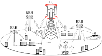
Figure 1: Heterogeneous Wireless Network: base station (BS), remote radio head (RRH) and wireless sensor networks (WSN).

5G cellular networks will be able to support a large number and diverse classes of devices, i.e., they will be heterogeneous, where a single macro cell may need to support 10,000 or more low-rate devices, along with its traditional high-rate mobile users [36]. This will require joint user classification according to their data rate requirements. Thus, a user in a high definition video call may have higher data rate requirements compared to a mobile user transmitting voice. Then we can classify them in different classes of users. In this section, a signal model for heterogeneous networks with different classes of users and an arbitrary configuration of CAS and DAS is presented. We consider the uplink channel scenario of a massive MIMO system with $N$ different classes of active users transmitting simultaneously signals to one base station (BS) equipped with $D$ remote antenna arrays distributed around the cell and $N_{B}$ receive antennas at the BS. Each remote array of antennas has $Q$ antennas linked to the BS via wired links. Therefore, the total number of receive antennas is $N_{r}=N_{B}+DQ$. The choice of $N_{B}$, $D$ and $Q$ is made based on the features of the network and type of application scenario. For example, suppose that we have a city with a high density of users or devices in the centre of a cell and sparsely distributed users or devices in the remaining part of the cell. In this case, we could use a number of centralized antennas to deal with the high density of users and distributed antennas to serve the remaining devices. The cardinality of the $n$-th user class $\mid C_{n}\mid$, represents the number of users of the class $n$. The total number of active users is given by $K=\sum_{n=1}^{N}\mid C_{n}\mid$. The $k$-th user in the $n$-th user class transmits data divided into $N_{t_{k,n}}$ sub-streams through $N_{t_{k,n}}$ antennas, where $N_{r}\geqslant N_{t}=\sum_{n=1}^{N}\sum_{k=1}^{\mid C_{n}\mid}N_{t_{k,n}}$ and $N_{t}$ is the total number of transmit antennas. The received signal vector at the BS from all active users in all user classes is given by

$$\mathbf{y}=\sum_{n=1}^{N}\sum_{k=1}^{\mid C_{n}\mid}\mathbf{\Upsilon}_{k,n}\bar{\mathbf{H}}_{k,n}\mathbf{s}_{k,n}+\mathbf{n},$$ (1)

where $\mathbf{s}_{k,n}$ is the $N_{t_{k,n}}\times 1$ transmitted signal vector, by the $k$-th user of the $n$-th user class, at one time slot taken from a complex constellation, denoted by $\mathcal{A}=\{a_{1},a_{2},\ldots,a_{O}\}$. Each symbol has $M$ bits and $O=2^{M}$. The vector $\mathbf{n}$ is an $N_{r}\times 1$ zero mean complex circular symmetric Gaussian noise vector with covariance matrix $\mathbf{K}_{\mathbf{n}}=\mathbb{E}[\mathbf{n}\mathbf{n}^{\mathcal{H}}]=\sigma_{n}^{2}\mathbf{I}$. Moreover, $\bar{\mathbf{H}}_{k,n}$ is the $N_{r}\times N_{t_{k,n}}$ channel matrix of the $k$-th user in the class $n$ with elements $\bar{h}_{i,j}^{(k,n)}$ corresponding to the complex channel gain from the $j$-th transmit antenna of the $k$-th user to the $i$-th receive antenna. For the antenna elements located at the BS and at each remote radio head, the $D+1$ sub-matrices of $\bar{\mathbf{H}}_{k,n}=[(\bar{\mathbf{H}}_{k,n}^{(1)})^{T},(\bar{\mathbf{H}}_{k,n}^{(2)})^{T},\ldots,(\bar{\mathbf{H}}_{k,n}^{(D+1)})^{T}]^{T}$ can be modeled using the Kronecker channel model [37], expressed by

$$\bar{\mathbf{H}}_{k,n}^{(j)}=(\mathbf{R}^{(j)}_{r})^{1/2}\mathbf{G}_{k,n}^{(j)}(\mathbf{R}_{t_{k,n}})^{1/2}$$ (2)

where $\mathbf{G}_{k,n}^{(j)}$ has complex channel gains between the $k$-th user and the $j$-th radio head, obtained from an independent and identically distributed random fading model whose coefficients are complex Gaussian random variables with zero mean and unit variance. $\mathbf{R}_{r}^{(j)}$ and $\mathbf{R}_{t_{k,n}}$ denote the receive correlation matrix of the $j$-th radio head and the transmit correlation matrix, respectively. The components of the correlation matrices $\mathbf{R}_{r}^{(j)}$ and $\mathbf{R}_{t_{k,n}}$ are of the form:

$$\mathbf{R}=\begin{bmatrix}1&\rho&\rho^{4}&\ldots&\rho^{(N_{a}-1)^{2}}\\ \rho&1&\rho&\ldots&\vdots\\ \rho^{4}&\rho&1&\vdots&\rho^{4}\\ \vdots&\vdots&\vdots&\vdots&\vdots\\ \rho^{(N_{a}-1)^{2}}&\ldots&\rho^{4}&\rho&1\end{bmatrix},$$ (3)

where $N_{a}$ is the number of antennas and $\rho$ is the correlation coefficient of neighboring antennas ($\rho=\rho_{t_{x}}$ for the transmit antennas and $\rho=\rho_{r_{x}}$ for the receive antennas). Note that $\rho=0$ represents an uncorrelated scenario and $\rho=1$ implies a fully correlated scenario. The $N_{r}\times N_{r}$ diagonal matrix $\mathbf{\Upsilon}_{k,n}$ represents the large-scale propagation effects for the user $k$ of the user class $n$, such as path loss and shadowing, given by

$$\mathbf{\Upsilon}_{k,n}=\text{diag}\Big{(}\underbrace{\gamma^{1}_{k,n}\ldots\gamma^{1}_{k,n}}_{N_{B}}\underbrace{\gamma^{2}_{k,n}\ldots\gamma^{2}_{k,n}}_{Q}\ldots\underbrace{\gamma^{D+1}_{k,n}\ldots\gamma^{D+1}_{k,n}}_{Q}\Big{)},$$ (4)

where the parameters $\gamma_{k,n}^{j}$ denote the large-scale propagation effects from the $k$-th user to the $j$-th radio head described by

$$\gamma_{k,n}^{j}=\alpha_{k,n}^{j}\beta_{k,n}^{j},\,\,\,\,\,\,\,j=1,\ldots,D+1.$$ (5)

Here $\alpha_{k,n}^{j}$ is the distance based path-loss between each user and the radio heads which is calculated by

$$\alpha_{k,n}^{j}=\sqrt{\frac{L_{k,n}^{j}}{(d_{k,n}^{j})^{\tau}}},$$ (6)

where $L_{k,n}^{j}$ is the power path loss of the link associated with the user and the $j$-th radio head, $d_{k,n}^{j}$ is the relative distance between this user and the $j$-th radio head, $\tau$ is the path loss exponent chosen between 2 and 4 depending on the environment. The log normal random variable $\beta_{k,n}^{j}$ which represents the shadowing between user $k$ and the receiver is given by

$$\beta_{k,n}^{j}=10^{\frac{\mu_{k,s}\vartheta^{j}_{k,s}}{10}},$$ (7)

where $\mu_{k,s}$ is the shadowing spread in dB and $\vartheta^{j}_{k,s}$ corresponds to a real-valued Gaussian random variable with zero mean and unit variance. Since the $N_{r}\times N_{t_{k,n}}$ composite channel matrix includes large-scale and small-scale fading effects it can be denoted as $\mathbf{H}_{k,n}=\mathbf{\Upsilon}_{k,n}\bar{\mathbf{H}}_{k,n}$, and the expression in (1) can be written as

$$\mathbf{y} = \sum_{n=1}^{N}\mathbf{H}_{n}\mathbf{s}_{n}+\mathbf{n},$$ (8)

where $\mathbf{H}_{n}=[\mathbf{H}_{1,n}\,\,\,\mathbf{H}_{2,n}\ldots\mathbf{H}_{\mid C_{n}\mid,n}]$ and $\mathbf{s}_{n}=[\mathbf{s}_{1,n}^{T}\,\,\,\mathbf{s}_{2,n}^{T}\ldots\mathbf{s}_{\mid C_{n}\mid,n}^{T}]^{T}$ represent the channel matrix and the transmitted symbol vector of all users in the class $n$, respectively. The received signal vector can be expressed more conveniently as

$$\mathbf{y} = \mathbf{H}\mathbf{s}+\mathbf{n},$$ (9)

where $\mathbf{H}=[\mathbf{H}_{1}\,\,\,\mathbf{H}_{2}\ldots\mathbf{H}_{N}]$ and $\mathbf{s}=[\mathbf{s}_{1}^{T}\,\,\,\mathbf{s}_{2}^{T}\ldots\mathbf{s}_{N}^{T}]^{T}$. The symbol vector $\mathbf{s}$ of all $N$ user classes has zero mean and a covariance matrix $\mathbf{K}_{\mathbf{s}}=\mathbb{E}[\mathbf{s}\mathbf{s}^{\mathcal{H}}]=\text{diag}(\mathbf{p})$, where the elements of the vector $\mathbf{p}$ are the signal power of each transmit antenna. To maintain a notational simplicity in the subsequent analysis, we assume that all antenna elements at the users transmit with the same average transmitted power $\sigma_{s}^{2}$, i.e., $\mathbf{K}_{\mathbf{s}}=\sigma_{s}^{2}\mathbf{I}$. We assume that the channel matrix $\mathbf{H}$ was previously estimated at the BS. From (9) we can see that the signals arrive coupled at the BS. If we want to use different detection procedures for each user class according to its data requirements, we have to separate the received signal vector $\mathbf{y}$ into independent received signals for each user class. For the system model presented in this work, when the number of remote radio heads is set to zero, i.e., $D=0$, the DAS architecture is reduced to the CAS scheme with $N_{r}=N_{B}$.

III Decoupled Signal Detection

As presented in Section II, in heterogeneous networks different classes of users send parallel data streams, through the massive MIMO channel operating with distributed antennas, which arrive superposed at the BS. In this 5G context, we need to separate the data streams for each category of users efficiently. In this section, we describe the proposed decoupled signal detection (DSD) which allows us to separate the received signal of the $n$-th user class from the others. To this end, we consider that the process of authentication, identification and channel estimation was already made, i.e, the BS is able to identify the users by classes according to their data requirements. Similar approaches to the proposed DSD algorithm have been proposed for the downlink, such as block diagonalization (BD) based techniques [38]-,[41],[42],[43][44] and other advanced precoding techniques [45]. However, unlike prior work in which downlink BD is used, for the proposed DSD scheme it is not necessary to use any precoding at the transmit side. The receiver only needs to know the channels between users and receive antennas. Moreover, the concept of separating the users with respect to the classes in heterogeneous networks according to its requirements is a new approach. The first steps to construct the concept proposed in this paper were presented in [1][46]. The received signal vector (8) can be written as:

$$\mathbf{y} = \mathbf{H}_{n}\mathbf{s}_{n}+\sum_{m=1,m\neq n}^{N}\mathbf{H}_{m}\mathbf{s}_{m}+\mathbf{n},$$ (10)

where $\mathbf{H}_{n}$ and $\mathbf{s}_{n}$ are the channel matrix and the transmitted symbol vector for the $n$-th user class, respectively. From (10), we can see that the $n$-th user class has inter-user class interference.

III-A Proposed Decoupling Strategy

To remove the presence of the other classes of users in the detection procedure for the $n$-th user class, we can employ a linear operation to project the received signal vector $\mathbf{y}$ onto the subspace orthogonal or almost orthogonal to the subspace generated by the signals of the interfering classes. In DSD, a matrix $\mathbf{A}_{n}$ is calculated employing a channel inversion method and a QR decomposition [47] [48], in order to decouple the $n$-th user’s class received signal from other user’s class signals. To compute $\mathbf{A}_{n}$, we construct the matrix $\tilde{\mathbf{H}}_{n}$ excluding the channel matrix of the $n$-th user class in the following form:

$$\tilde{\mathbf{H}}_{n}=[\mathbf{H}_{1}\ldots\mathbf{H}_{n-1}\,\,\,\mathbf{H}_{n+1}\ldots\mathbf{H}_{N}],$$ (11)

where $\tilde{\mathbf{H}}_{n}\in\mathbb{C}^{N_{r}\times(N_{t}-N_{t_{n}})}$ and $N_{t_{n}}=\sum_{k=1}^{\mid C_{n}\mid}N_{t_{k,n}}$ is the number of transmit antennas in the $n$-th user class. After that, the objective is to obtain a matrix $\mathbf{A}_{n}$ that satisfies the following condition:

$$\mathbf{A}_{n}\tilde{\mathbf{H}}_{n}=\mathbf{0},\,\,\,\,\,\forall n\in(1\ldots N).$$ (12)

To compute $\mathbf{A}_{n}$, DSD first computes the MMSE channel inversion of the combined channel matrix $\mathbf{H}$ given by

$$\mathbf{H}^{\dagger} = \mathbf{H}^{\mathcal{H}}(\mathbf{H}\mathbf{H}^{\mathcal{H}}+\sigma^{2}\mathbf{I})^{-1}$$ (13)

$$= [(\ddot{\mathbf{H}}_{1})^{T}\,\,\,(\ddot{\mathbf{H}}_{2})^{T}\,\,\,\ldots\,\,\,(\ddot{\mathbf{H}}_{N})^{T}]^{T}$$

where $\sigma^{2}=\sigma_{n}^{2}/\sigma_{s}^{2}$, $\mathbf{H}^{\dagger}\in\mathbb{C}^{N_{t}\times N_{r}}$ and $\ddot{\mathbf{H}}_{n}\in\mathbb{C}^{N_{t_{n}}\times N_{r}}$. Then, the matrix $\ddot{\mathbf{H}}_{n}$ is approximately in the null space of $\tilde{\mathbf{H}}_{n}$, that is

$$\ddot{\mathbf{H}}_{n}\tilde{\mathbf{H}}_{n}\approx\mathbf{0},\,\,\,\,\,\forall n\in(1\ldots N).$$ (14)

To decouple the $n$-th user group from the other user groups we employ a QR decomposition as described by

$$\ddot{\mathbf{H}}_{n}=\mathbf{R}_{n}\mathbf{Q}_{n},\,\,\,\,\,\forall n\in(1\ldots N),$$ (15)

where $\mathbf{R}_{n}\in\mathbb{C}^{N_{t_{n}}\times N_{t_{n}}}$ is an upper triangular matrix and $\mathbf{Q}_{n}\in\mathbb{C}^{N_{t_{n}}\times N_{r}}$ is a matrix with orthogonal rows and composed by approximately orthonormal basis vectors of the left null space of $\tilde{\mathbf{H}}_{n}$. Then we have

$$\mathbf{Q}_{n}\tilde{\mathbf{H}}_{n}\approx\mathbf{0}.$$ (16)

From (16), we can see that $\mathbf{Q}_{n}$ is a good approximation for $\mathbf{A}_{n}$ in (12). Using $\mathbf{A}_{n}=\mathbf{Q}_{n}$ as a linear combination with the received signal vector in (10), we have

$$\mathbf{y}_{n} = \mathbf{A}_{n}\mathbf{y}$$ (17)

$$= \mathbf{Q}_{n}\mathbf{H}_{n}\mathbf{s}_{n}+\mathbf{Q}_{n}\sum_{\begin{subarray}{c}m=1\\ m\neq n\end{subarray}}^{N}\mathbf{H}_{m}\mathbf{s}_{m}+\mathbf{Q}_{n}\mathbf{n},$$

where $\mathbf{y}_{n}\in\mathbb{C}^{N_{t_{n}}\times 1}$ is the equivalent received signal vector for the user class $n$ and the term $\mathbf{Q}_{n}{\sum_{\begin{subarray}{c}m=1\\ m\neq n\end{subarray}}^{N}}\mathbf{H}_{m}\mathbf{s}_{m}\approx\mathbf{0}$ represents the residual inter-user class interference. Then, we can transform the received signal vector into parallel single-user class signals as described by

$$\mathbf{y}_{n}=\check{\mathbf{H}}_{n}\mathbf{s}_{n}+\mathbf{n}_{n},\,\,\,\,\,\forall n\in(1\ldots N),$$ (18)

where $\check{\mathbf{H}}_{n}=\mathbf{Q}_{n}\mathbf{H}_{n}\in\mathbb{C}^{N_{t_{n}}\times N_{t_{n}}}$ is the equivalent channel matrix of the $n$-th user class after DSD and $\mathbf{n}_{n}=\mathbf{Q}_{n}{\sum_{\begin{subarray}{c}m=1\\ m\neq n\end{subarray}}^{N}}\mathbf{H}_{m}\mathbf{s}_{m}+\mathbf{Q}_{n}\mathbf{n}\in\mathbb{C}^{N_{t_{n}}\times 1}$ is the equivalent noise vector.

Another option to compute a basis for the left null space of $\tilde{\mathbf{H}}_{n}$ is performing the SVD transformation $\tilde{\mathbf{H}}_{n}=\tilde{\mathbf{U}}_{n}\tilde{\mathbf{\Sigma}}_{n}\tilde{\mathbf{V}}_{n}^{\mathcal{H}}$, where $\tilde{\mathbf{\Sigma}}_{n}\in\mathbb{C}^{N_{r}\times(N_{t}-N_{t_{n}})}$ is a rectangular diagonal matrix with the singular values of $\tilde{\mathbf{H}}_{n}$ on the diagonal, $\tilde{\mathbf{U}}_{n}\in\mathbb{C}^{N_{r}\times N_{r}}$ and $\tilde{\mathbf{V}}_{n}^{\mathcal{H}}\in\mathbb{C}^{(N_{t}-N_{t_{n}})\times(N_{t}-N_{t_{n}})}$ are unitary matrices. If $r_{n}$ is the rank of $\tilde{\mathbf{H}}_{n}$, that corresponds to the number of non-zero singular values, i.e., $r_{n}={\rm rank}(\tilde{\mathbf{H}}_{n})\leq N_{t}-N_{t_{n}}$, the SVD can be expressed equivalently as:

$$\tilde{\mathbf{H}}_{n}=[\tilde{\mathbf{U}}_{1,n}\,\,\,\tilde{\mathbf{U}}_{0,n}]\,\,\,\tilde{\mathbf{\Sigma}}_{n}\,\,\,[\tilde{\mathbf{V}}_{1,n}\,\,\,\tilde{\mathbf{V}}_{0,n}]^{\mathcal{H}},$$ (19)

where $\tilde{\mathbf{U}}_{0,n}~{}\in~{}\mathbb{C}^{N_{r}\times(N_{r}-r_{n})}$ and $\tilde{\mathbf{V}}^{\mathcal{H}}_{0,n}~{}\in~{}\mathbb{C}^{(N_{t}-N_{t_{n}}-r_{n})\times(N_{t}-N_{t_{n}})}$ form an orthogonal basis for the left null space and the null space of $\tilde{\mathbf{H}}_{n}$, respectively. Then, the alternative solution for (12) could be:

$$\mathbf{A}_{n}=\tilde{\mathbf{U}}_{0,n}^{\mathcal{H}}.$$ (20)

Although the matrix $\tilde{\mathbf{U}}_{0,n}^{\mathcal{H}}$ eliminates the inter-user class interference effectively, i.e., $\tilde{\mathbf{U}}_{0,n}^{\mathcal{H}}{\sum_{\begin{subarray}{c}m=1\\ m\neq n\end{subarray}}^{N}}\mathbf{H}_{m}\mathbf{s}_{m}=\mathbf{0}$, the linear combination $\mathbf{y}_{n}=\tilde{\mathbf{U}}_{0,n}^{\mathcal{H}}\mathbf{y}$ presents a noise enhancement in the detection procedures which reduces the performance. In the first approach, when we use $\mathbf{y}_{n}=\mathbf{Q}_{n}\mathbf{y}$, the noise enhancement in the detection procedures is mitigated due to the fact that the equivalent noise vector has a lower dimension when compared with the other option. Thus, the noise enhancement is reduced which improves the performance, even in the presence of residual interference. In addition, the equivalent channel matrix $\check{\mathbf{H}}_{n}^{1}=\tilde{\mathbf{U}}_{0,n}^{\mathcal{H}}\mathbf{H}_{n}$ has dimensions $(N_{r}-r)\times N_{t}$ against the matrix $\check{\mathbf{H}}_{n}^{2}=\mathbf{Q}_{n}\mathbf{H}_{n}$ which has dimensions $N_{t_{n}}\times N_{t_{n}}$. For this reason the computational complexity of the detector is lower if we use the matrix $\mathbf{Q}_{n}$ to decouple the received signal vector.

The fact that we obtain a square equivalent channel matrix also allows the possibility of using lattice reduction (LR) based detectors which have a better performance for square channel matrices [49]. Further, the computational complexity to compute the channel inversion (13) and $N$ QR decompositions (15) of matrices with dimensions $N_{t_{n}}\times N_{r}$ is much lower than the computational cost of computing $N$ SVD transformations (19) of matrices with dimensions $N_{r}\times(N_{t}-N_{t_{n}})$. For these reasons, in this paper we will focus on the first alternative.

As it will be presented in next section, the equivalent received signal vector in (18) shows that the process in (11)-(17) is an effective algorithm to separate the user classes at the BS and we can consider the data stream of the $n$-th user class as independent of the received signals of the other user classes. In practice, this allows the possibility of using different transmission and reception schemes for each user class. We can now implement the traditional detectors for each class of users separately which also allows the possibility of using more complex detection schemes due to the reduction of the dimensions of the matrices that need to be processed. The description of the proposed DSD algorithm is presented in Algorithm 1.

III-B Detection Algorithms

In this subsection, we examine signal detection algorithms for massive MIMO in heterogeneous networks. To detect the data stream for each class of users independently, we assume that the DSD algorithm described in Algorithm 1 was previously employed.

III-B1 Linear Detectors

In linear detectors, the equivalent received signal vector for the $n$-th user class $\mathbf{y}_{n}\in\mathbb{C}^{N_{t_{n}}\times 1}$ is processed by a linear filter to eliminate the channel effects [50]. The two linear detectors considered here are given by

$$\mathbf{W}_{n}^{\chi}=\begin{cases}(\check{\mathbf{H}}_{n}^{\mathcal{H}}\check{\mathbf{H}}_{n})^{-1}\check{\mathbf{H}}_{n}^{\mathcal{H}},&\chi=\text{Zero Forcing }\\ (\check{\mathbf{H}}_{n}^{\mathcal{H}}\check{\mathbf{H}}_{n}+\sigma^{2}\mathbf{I})^{-1}\check{\mathbf{H}}_{n}^{\mathcal{H}},&\chi=\text{MMSE}\end{cases}$$ (21)

where $\sigma^{2}=\sigma_{n}^{2}/\sigma_{s}^{2}$ and $\check{\mathbf{H}}_{n}\in\mathbb{C}^{N_{t_{n}}\times N_{t_{n}}}$ is the equivalent channel matrix of the $n$-th user class. Note that for the MMSE detector, we consider the autocorrelation matrix of the equivalent noise vector as $\mathbf{K}_{\mathbf{n}_{n}}\approx\sigma_{n}^{2}\mathbf{I}$. As the residual interference is very small, an excellent performance can be obtained with this approximation. The linear hard decision of $\mathbf{s}_{n}$ is carried out as follows:

$$\hat{\mathbf{s}}_{n}=\mathbb{C}(\mathbf{W}_{n}^{\chi}\mathbf{y}_{n}),$$ (22)

where the function $\mathbb{C}(x)$ returns the point of the complex signal constellation closest to $x$. The linear detectors have a lower computational complexity when compared with the non-linear detectors. However, due to the impact of interference and noise, linear detectors offer a limited performance.

III-B2 Successive Interference Cancellation (SIC)

The SIC detector for the $n$-th user class in (18) consists of a bank of linear detectors, each detects a selected component $s_{n,i}$ of $\mathbf{s}_{n}$. The component obtained by the first detector is used to reconstruct the corresponding signal vector which is then subtracted from the equivalent received signal to further reduce the interference in the input to the next linear receive filter. The successively canceled received data vector that follows a chosen ordering in the $i$-th stage is given by

$$\mathbf{y}_{n,i}=\mathbf{y}_{n}-\sum_{j=1}^{i-1}\check{\mathbf{h}}_{n,j}\hat{s}_{n,j},$$ (23)

where $\check{\mathbf{h}}_{n,j}$ correspond to the columns of the channel matrix $\check{\mathbf{H}}_{n}$ and $\hat{s}_{n,j}$ is the estimated symbol obtained at the output of the $j$-th linear detector.

III-B3 Multiple-Branch SIC Detection

In the multi-branch scheme [25] for the $n$-th user class, different orderings are explored for SIC, each ordering is referred to as a branch, so that a detector with $L$ branches produces a set of $L$ estimated vectors. Each branch uses a column permutation matrix $\mathbf{P}_{n}$. The estimate of the signal vector of branch $l$, $\mathbf{\hat{x}}_{n}^{(l)}$, is obtained using a SIC receiver based on a new channel matrix $\check{\mathbf{H}}_{n}^{(l)}=\check{\mathbf{H}}_{n}\mathbf{P}_{n}^{(l)}$. The order of the estimated symbols is rearranged to the original order by

$$\mathbf{\hat{s}}_{n}^{(l)}=\mathbf{P}_{n}^{(l)}\mathbf{\hat{x}}_{n}^{(l)},\,\,\,\,\,\,\,l=1,\ldots,L.$$ (24)

A higher detection diversity can be obtained by selecting the most likely symbol vector based on the ML selection rule, that is

$$\mathbf{\hat{s}}_{n}=\text{arg min}\parallel\mathbf{y}_{n}-\check{\mathbf{H}}_{n}\mathbf{\hat{s}}_{n}^{l}\parallel^{2},\hskip 14.22636ptl=1,\ldots,L.$$ (25)

Other detectors could be used with the proposed DSD technique and this is up to the designer to choose the detector.

IV Sum-Rate Analysis

$$R_{k,n}=\mathbb{E}\Bigg{[}\log_{2}\Bigg{(}1+\frac{\sigma_{s}^{2}\mid\mathbf{w}_{k,n}\check{\mathbf{h}}_{k,n}\mid^{2}}{\sigma_{s}^{2}\sum_{\begin{subarray}{c}j=1\\ j\neq k\end{subarray}}^{\mid C_{n}\mid}\mid\mathbf{w}_{k,n}\check{\mathbf{h}}_{j,n}\mid^{2}+\mid\mathbf{w}_{k,n}[\sigma_{s}^{2}\mathbf{Q}_{n}(\sum_{\begin{subarray}{c}m=1\\ m\neq n\end{subarray}}^{N}\mathbf{H}_{m}\mathbf{H}_{m}^{\mathcal{H}})\mathbf{Q}_{n}^{\mathcal{H}}+\sigma_{n}^{2}\mathbf{I}]\mathbf{w}_{k,n}^{\mathcal{H}}\mid}\Bigg{)}\Bigg{]},$$ (35)

In this section, a performance analysis for the proposed DSD scheme is presented in terms of the sum rate. We consider that the channel matrix $\mathbf{H}$ was previously estimated at the BS, assume Gaussian signalling and that the received signal vector was decoupled for each user class. Considering the received signal vector as presented in (18), the sum rate [51] that DSD can offer is defined as

$$R=\sum_{n=1}^{N}\log_{2}\frac{\det(\mathbf{K}_{\mathbf{y}_{n}})}{\det(\mathbf{K}_{\mathbf{n}_{n}})},$$ (26)

where $\mathbf{K}_{\mathbf{y}_{n}}$ and $\mathbf{K}_{\mathbf{n}_{n}}$ are the autocorrelation matrix of the equivalent received signal vector and the equivalent noise vector of the $n$-th user class, respectively. It is easy to show that (26), can be expressed as

$$R=\sum_{n=1}^{N}\log_{2}\det(\mathbf{I}+\mathbf{B}_{n}\mathbf{B}_{n}^{\mathcal{H}}),$$ (27)

where $\mathbf{B}_{n}=\mathbf{K}_{\mathbf{n}_{n}}^{-1/2}\check{\mathbf{H}}_{s}\mathbf{K}_{\mathbf{s}_{n}}^{1/2}\in\mathbb{C}^{N_{t_{n}}\times N_{t_{n}}}$. As $\mathbf{B}_{n}\mathbf{B}_{n}^{\mathcal{H}}$ is a Hermitian symmetric positive-definite square matrix, we have

$$\mathbf{B}_{n}\mathbf{B}_{n}^{\mathcal{H}}=\bar{\mathbf{Q}}_{n}\mathbf{\Lambda}_{n}\bar{\mathbf{Q}}_{n}^{\mathcal{H}},$$ (28)

where $\bar{\mathbf{Q}}_{n}$ is a square unitary matrix, $\bar{\mathbf{Q}}_{n}\bar{\mathbf{Q}}_{n}^{\mathcal{H}}=\mathbf{I}$, and $\mathbf{\Lambda}_{n}$ is a diagonal matrix whose diagonal elements are the eigenvalues of the matrix $\mathbf{B}_{n}\mathbf{B}_{n}^{\mathcal{H}}$. Then, the reliable sum rate that the system can offer is

$$R=\sum_{n=1}^{N}\sum_{i=1}^{N_{t_{n}}}\log_{2}(1+\lambda_{i,n}).$$ (29)

Note that the eigenvalues $\lambda_{i,n}$ in (29) can be obtained computing the eigenvalues of $\mathbf{B}_{n}^{\mathcal{H}}\mathbf{B}_{n}$. As mentioned before, for notational simplicity we assume that $\mathbf{K}_{\mathbf{s}_{n}}=\sigma_{s}^{2}\mathbf{I}$. When the DSD algorithm is applied, the equivalent noise vector for the $n$-th user class $\mathbf{n}_{n}={\mathbf{Q}_{n}\sum_{\begin{subarray}{c}m=1\\ m\neq n\end{subarray}}^{N}\mathbf{H}_{m}\mathbf{s}_{m}+\mathbf{Q}_{n}\mathbf{n}}\in\mathbb{C}^{N_{t_{n}}\times 1}$ is not white due to the residual inter-user class interference. Then its autocorrelation matrix is given by

$$\mathbf{K}_{\mathbf{n}_{n}}=\mathbb{E}[\mathbf{n}_{n}\mathbf{n}_{n}^{\mathcal{H}}]=\sigma_{s}^{2}\mathbf{Q}_{n}\Big{(}\sum_{\begin{subarray}{c}m=1\\ m\neq n\end{subarray}}^{N}\mathbf{H}_{m}\mathbf{H}_{m}^{\mathcal{H}}\Big{)}\mathbf{Q}_{n}^{\mathcal{H}}+\sigma_{n}^{2}\mathbf{I}.$$ (30)

Finally, the eigenvalues $\lambda_{i,n}$ in (29) are obtained from the eigenvalues of matrix $\mathbf{B}_{n}^{\mathcal{H}}\mathbf{B}_{n}$ given by

$$\mathbf{B}_{n}^{\mathcal{H}}\mathbf{B}_{n}=\frac{\sigma_{s}^{2}}{\sigma_{n}^{2}}\check{\mathbf{H}}_{n}^{\mathcal{H}}\Big{[}\frac{\sigma_{s}^{2}}{\sigma_{n}^{2}}\mathbf{Q}_{n}\Big{(}\sum_{\begin{subarray}{c}m=1\\ m\neq n\end{subarray}}^{N}\mathbf{H}_{m}\mathbf{H}_{m}^{\mathcal{H}}\Big{)}\mathbf{Q}_{n}^{\mathcal{H}}+\mathbf{I}\Big{]}^{-1}\check{\mathbf{H}}_{n}.$$ (31)

To compute the sum rate for the received signal vector in (9) when the detection is perform for all user classes together, we suppress the index $n$ from the above analysis and considering that $\mathbf{K}_{\mathbf{s}}=\sigma^{2}_{s}\mathbf{I}$ and $\mathbf{K}_{\mathbf{n}}=\sigma_{n}^{2}\mathbf{I}$, we get the well-known expression:

$$\bar{R}=\sum_{i=1}^{N_{t}}\log_{2}(1+\lambda_{i}),$$ (32)

where the values $\lambda_{i}$ are the eigenvalues of the matrix $\mathbf{B}^{\mathcal{H}}\mathbf{B}=\frac{\sigma^{2}_{s}}{\sigma_{n}^{2}}\mathbf{H}^{\mathcal{H}}\mathbf{H}$ [51]. In Appendix A, we show that, as well as the sum rate in (32) when all user classes are detected together, the sum rate in (29) for the proposed DSD algorithm is independent of the detection procedure. However, the lower bound on the achievable uplink sum rate obtained by using linear detectors is different for each detector [52]. In order to analyze the behavior of the lower bound on the sum rate for the proposed DSD scheme we consider that a linear detector according to (21) is applied to the equivalent received signal vector (18) to detect the transmitted symbol vector of the user class $n$, then we have

$$\tilde{\mathbf{y}}_{n}=\mathbf{W}_{n}\mathbf{y}_{n}=\mathbf{W}_{n}\check{\mathbf{H}}_{n}\mathbf{s}_{n}+\mathbf{W}_{n}\mathbf{n}_{n}.$$ (33)

Taking the $k$-th element of $\tilde{\mathbf{y}}_{n}$ we have

$$\tilde{y}_{k,n}=\mathbf{w}_{k,n}\check{\mathbf{h}}_{k,n}s_{k,n}+\sum_{\begin{subarray}{c}j=1\\ j\neq k\end{subarray}}^{\mid C_{n}\mid}\mathbf{w}_{k,n}\check{\mathbf{h}}_{j,n}s_{j,n}+\mathbf{w}_{k,n}\mathbf{n}_{n},$$ (34)

where $\mathbf{w}_{k,n}$ is the $k$-th row of $\mathbf{W}_{n}$. Modeling the noise interference, the inter-user class interference and the inter-user interference in the user class $n$ in (34) as additive Gaussian noise independent of $s_{k,n}$, considering (30) and that the channel is ergodic so that each codeword spans over a large number of realizations, we obtain the lower bound on the achievable rate for the DSD algorithm with linear detectors as described in (35). Then, the lower bound on the achievable rate for the entire system is given by

$$R=\sum_{n=1}^{N}\sum_{k=1}^{\mid C_{n}\mid}R_{k,n}.$$ (36)

For the SIC receiver, each stream is filtered by a linear detector and then, its contribution is subtracted from the received signal to improve the subsequent detection. For each layer the linear filter is recalculated. The performance of SIC detectors can be improved if we choose the cancellation order as a function of the SINR at the output of the linear detector in each layer. The lower bound for the sum rate of the proposed DSD algorithm when a SIC detector is used for each user class, could be calculated updating the expression (35) in each layer, i.e., the values of $\mathbf{w}_{k,n}$ are recalculated for each detected stream.

V Numerical Results

In this section, we evaluate the performance of the proposed DSD algorithm with different detectors in terms of the sum rate and the BER via simulations. Moreover, the computational complexity of the proposed and existing algorithms is also evaluated.

V-A Sum Rate

To evaluate the analytic results obtained in Section IV, the sum rate and the lower bounds for the proposed DSD algorithm with different detection schemes will be evaluated considering CAS and DAS configuration assuming perfect CSI. For the CAS configuration, we employ $L_{k}=0.7$, $\tau=2$, the distance $d_{k}$ to the BS is obtained from a uniform discrete random variable distributed between 0.1 and 0.99, the shadowing spread is $\sigma_{k}=3$ dB and the transmit and receive correlation coefficients are $\rho_{rx}=0.2$ and $\rho_{tx}=0.4$ (when $N_{t_{k,n}}>1$), respectively. For DAS configurations, we consider a densely populated cell, where a fraction of the active users are in the centre of the cell and the remaining users are in other locations of the cell. We explore different particular values for the fraction of users in the centre and around the cell. Based on that, we choose specific values for $N_{B}$, $D$ and $Q$. For the DAS configuration, we also consider $L_{k,j}$ taken from a uniform random variable distributed between 0.7 and 1, $\tau=2$, the distance $d_{k,j}$ for each link to an antenna is obtained from a uniform discrete random variable distributed between 0.1 and 0.5, the shadowing spread is $\sigma_{k,j}=3$ dB and the transmit and receive correlation coefficients are $\rho_{rx}=0.2$ and $\rho_{tx}=0.4$ , respectively.

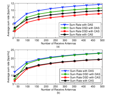
Figure 2: (a) Sum Rate vs Number of Receive antennas. N=4, $\mid C_{n}\mid=8$ users per class, $N_{t_{k,n}}=1$ antennas per user. (b) Sum Rate vs Number of Receive antennas. N=16, $\mid C_{n}\mid=1$ users per class, $N_{t_{k,n}}=2$ antennas per user.

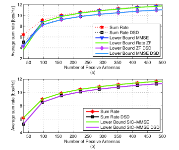
Figure 3: (a) Sum Rate vs Number of Receive antennas. N=3, $\mid C_{n}\mid=10$ users per class, $N_{t_{k,n}}=1$ antennas per user. (b) Sum Rate vs Number of Receive antennas. N=2, $\mid C_{n}\mid=16$ users per class, $N_{t_{k,n}}=1$ antennas per user.

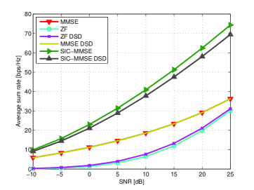
Figure 4: Sum Rate vs SNR. N=8, $\mid C_{n}\mid=1$ users per class, $N_{t_{k,n}}=8$ antennas per user. We consider DAS configuration with $N_{B}=96$, $D=4$ and $Q=8$.

In Fig. 2 we evaluate the sum rate in two different scenarios for the users requirements. In both cases, we fix the SNR=10 dB and increase the number of receive antennas. For the DAS configuration, we consider $N_{B}=1/2N_{r}$ antennas at the BS. We also consider $D=4$ arrays of antennas distributed around the cell, each equipped with $Q=1/8N_{r}$ antennas. For Fig. 2 (a) we consider $N=4$ classes of users with $\mid C_{n}\mid=8$ users each and $N_{t_{k,n}}=1$ antennas per user. We can see that the sum rate of the proposed DSD algorithm is close to the sum rate of the traditional MIMO system and with a low computational complexity on the detection procedures as will be shown in the next subsection. For Fig. 2 (b), we consider 16 active users in the system and that we need to detect each user independently, i.e., $N=16$ classes of users with $\mid C_{n}\mid=1$ users at each class and $N_{t_{k,n}}=2$ antennas per user. Under these conditions, the sum rate of the proposed scheme reaches the sum rate of the traditional MIMO system, especially for a large number of receive antennas. As expected, from the plot in Fig. 2, we can see that the sum rate for DAS is higher than that of the CAS configuration.

In Fig. 3, we compare the lower bound on the sum rate for different detectors such as, ZF, MMSE and SIC. We consider the DAS configuration under the same conditions as in the previous experiment. For Fig. 3 (a) we consider $N=3$ classes of users with $\mid C_{n}\mid=10$ users at each class and $N_{t_{k,n}}=1$ antennas per user. We can see from the plot, that similarly to the traditional MIMO systems, the lower bound on the sum rate for ZF and MMSE achieves the sum rate when $N_{r}$ grows. For Fig. 3 (b) we consider $N=2$ classes of users with $\mid C_{n}\mid=16$ users at each class and $N_{t_{k,n}}=1$ antennas per user. We can see that the SIC-MMSE achieves the sum rate and it could be considered optimal in terms of sum rate.

In Fig. 4, we compare the lower bound sum rate versus SNR. We consider $N=8$ classes of users with $\mid C_{n}\mid=1$ user in each class and $N_{t_{k,n}}=8$ antennas per user transmitting with high correlation between antennas $\rho_{tx}=0.85$. We consider the DAS configuration with $N_{B}=96$, $D=4$ and $Q=8$. We can see from the plot that the lower bounds for the proposed DSD algorithms are very close to the lower bounds when the detection procedure is carried out together for all users.

V-B Computational Complexity Analysis

In this subsection, the computational complexity of the proposed DSD algorithm is evaluated and compared with the traditional coupled detection schemes, when all user classes are detected together, by counting the number of floating point operations (FLOPs) per received vector $\mathbf{y}$. Different detection schemes are considered such as MMSE, SIC and MB-SIC. The SIC based receivers all use MMSE detection. Furthermore, the single-branch SIC and the first branch of the MB-SIC employ norm-based ordering. We consider QPSK modulation, however the computational cost in these detectors does not change significantly with the modulation order. The number of FLOPs for the complex QR decomposition of an $N_{t_{n}}\times N_{r}$ matrix is given in [53] as $16(N_{r}^{2}N_{t_{n}}-N_{t_{n}}^{2}N_{r}+1/3N_{t_{n}}^{3})$. To compute the number of FLOPs required for the remaining operations, we use the Light-speed Matlab toolbox [54].

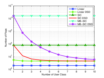
Figure 5: Computational complexity versus number of user class, $K=100$ active users, $N_{t_{k,n}}=2$ antennas per user, $N_{r}=200$ receive antennas.

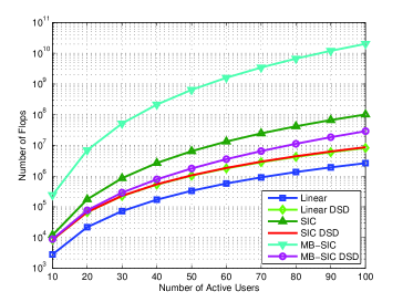
Figure 6: Computational complexity versus number of active user, $N=5$ classes of user, $N_{t_{k,n}}=2$ antennas per user, $N_{t}=KN_{t_{k,n}}$ transmit antennas and $N_{r}=3N_{t}$ receive antennas.

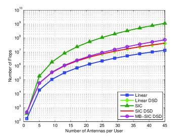
Figure 7: Computational complexity versus number of antennas per user, $K=10$ active user, $N=10$ classes of users, $N_{t}=KN_{t_{k,n}}$ transmit antennas and $N_{r}=2N_{t}$ receive antennas.

Fig. 5 shows the computational complexity versus the number of user classes for different detection algorithms. We consider $K=100$ active users, $N_{t_{k,n}}=2$ transmit antennas per user and $N_{r}=200$ receive antennas distributed around the cell. We consider an increasing number of classes of users, when $K$ is not divisible by the number of classes, the number of active users is set to a smaller value so as to allow the division in $N$ classes. We can see from the figure that the complexity of the SIC and the MB-SIC detectors with the DSD algorithm is lower than the SIC and the MB-SIC coupled detectors, respectively. Furthermore, for receivers with DSD the computational complexity is reduced as the number of user classes is increased. This fact represents an important advantage for receivers with DSD, due to the fact that it allows to use of more complex detectors for each user class according to its data requirements.

In Fig. 6 and Fig. 7 we plot the required number of FLOPs versus the number of active users and versus the number of antennas per user, respectively. For Fig. 6 we consider $N=5$ classes of users, $N_{t_{k,n}}=2$ transmit antennas per user and $N_{r}=3KN_{t_{k,n}}$ receive antennas. The MB-SIC and SIC detectors with DSD has a lower computational cost than the coupled SIC detector. For this 5G context, with a high number of antennas, efficient coupled detectors are not feasible to be implemented, however, if a specific user class requires the benefits of complex detectors, the DSD algorithm reduces the cost so that more complex detectors could be applied as illustrated with MB-SIC in Fig. 6. For the results in Fig. 7 we consider that we have $K=10$ active users and that we need to detect each user independently, i.e., $N=10$. The number of transmit antennas per user $N_{t_{k,n}}$ is increased. We also consider that the number of receive antennas distributed around the cell is given by $N_{r}=2KN_{t_{k,n}}$. The MB-SIC and SIC detectors with DSD have a significantly lower complexity when compared with the SIC detector where all users are coupled.

It is worth noting that the curves displayed in Fig. 5, Fig. 6 and Fig. 7 will have a substantial decrease if the channel does not change over a time period due to quasi static channels. In this case, the equivalent channel matrices for each user class are stored for subsequent use. It would increase the gap, in terms of the computational cost, for the detection schemes using the DSD algorithm.

V-C BER Performance

In this subsection, the BER performance of the proposed DSD algorithm is evaluated using different detectors which includes linear, SIC and MB-SIC with linear MMSE receive filters. The SIC detector of [21] uses a norm-based cancellation ordering, the MB-SIC of [25] employs a fixed number of branches, equal to the total number of transmit antennas per user class $N_{t_{n}}$ for the DSD schemes, and norm-based ordering in its first branch. A massive MIMO system operating in heterogeneous networks with $K$ active users is considered. We also consider the DAS configuration where the $N_{r}=N_{B}+DQ$ receive antennas are distributed around the cell in $D$ radio heads with $Q$ antennas each and the remaining $N_{B}$ antennas are located at the BS. We consider QPSK modulation. The SNR per transmitted information bit is defined as

$$\text{SNR}=10\log_{10}\frac{N_{t}\sigma_{s}^{2}}{M\sigma_{n}^{2}},$$ (37)

where $\sigma_{s}^{2}$ is the common variance of the transmitted symbols, $\sigma_{n}^{2}$ is the noise variance at the receiver and $M$ is the number of transmitted bits per symbol. The numerical results correspond to an average of 3,000 simulations runs, with 500$N_{t}$ symbols transmitted per run. For the $N_{B}$ antennas at the BS, we employ $L_{k}=0.3$, $\tau=2$, the distance to the users is obtained from a uniform discrete random variable distributed between 0.4 and 0.7, the shadowing spread is $\sigma_{k}=1$ dB and the transmit and receive correlation coefficients are equal to $\rho_{rx}=0.4$. For the $R$ remote arrays of antennas, we use $L_{k,j}$ taken from a uniform random variable distributed between 0.3 and 0.5, the shadowing spread $\sigma_{k,j}=1$ dB and the receive correlation coefficients are equal to $\rho_{rx}=0.5$. When the number of transmit antennas at the users is $N_{t_{k,n}}>1$, the transmit correlation coefficient is equal to $\rho_{tx}=0.55$.

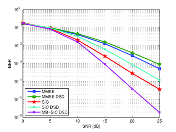
Figure 8: BER versus SNR with $K=12$ active users, $N=3$ classes of users, $N_{t_{k,n}}=3$ transmit antennas per user and $N_{r}=36$ receive antennas.

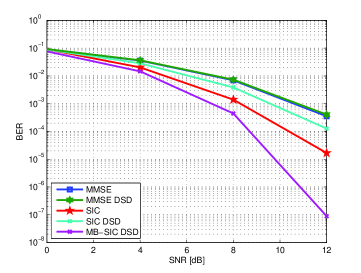
Figure 9: BER versus SNR with $K=8$ active users, $N_{t_{k,n}}=8$ transmit antennas per user, $N=8$ classes of users and $N_{r}=128$ receive antennas.

For the experiment in Fig. 8, we consider $K=12$ user devices, where each user is equipped with $N_{t_{k,n}}=3$ transmit antennas and $N=3$ classes of users. The system employs perfect channel state information and QPSK modulation. For the DAS configuration, we consider $N_{B}=8$ receive antennas at the BS, $D=4$ remote radio heads and $Q=7$ receive antennas per remote radio head. We can see from the figure that the decoupled SIC detection presents a performance close to the coupled SIC detector with a difference around 2 dB in the high SNR region. In addition the decoupled SIC detector has a drastic reduction in the computational cost when compared with its coupled version. The result also indicates a remarkable superiority in the performance for the MB-SIC receiver with the DSD scheme over the coupled SIC detector which also has a lower computational complexity than the coupled SIC detector.

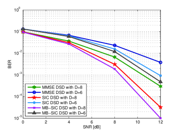
Figure 10: BER versus SNR with $K=64$ active users, $N_{t_{k,n}}=1$ transmit antennas per user, $N=4$ classes of users, $N_{B}=34$, $D$ remote antennas arrays with $Q=7$ receive antennas per array.

In the next example, we evaluate the performance of the proposed DSD scheme considering $K=8$ active users, each user transmitting with $N_{t_{k,n}}=8$ antennas. We also consider that we need to detect each user independently of each other, i.e., $N=8$ classes of users with $\mid C_{n}\mid=1$ users per class. For the DAS configuration, we consider $N_{B}=64$ receive antennas at the BS, $D=8$ remote radio heads and $Q=8$ receive antennas per remote radio head. The Fig. 9 indicate that the performance of the SIC detector with DSD is close to the SIC detector with a lower computational complexity. Note that the results for MB-SIC with DSD show a very good performance with a computational complexity much lower than the SIC detector without DSD.

In Fig. 10 we evaluate the performance of the proposed DSD scheme with MMSE, SIC and MB-SIC detection. We consider $K=64$ active users, $N=4$ classes of users, $\mid C_{n}\mid=16$ users per class and $N_{t_{k,n}}=1$ transmit antennas per user. For the DAS configuration, we consider $N_{B}=34$ receive antennas at the BS and $Q=7$ receive antennas per remote radio head. To show the behavior of the BER performance with different numbers of distributed antennas we consider two configurations of remote radios heads, $D=8$ and $D=6$. As expected, the results shows that when the number of RRHs is increased, the BER performance is improved due to the low propagation effects caused by the short distances between users and some remote antenna arrays. We also can see from the figure that the SIC and the MB-SIC detector with DSD offer an excellent BER performance with a low computational cost.

VI Conclusions

In this paper a mathematical signal model and the DSD algorithm for the uplink of massive MIMO systems operating in heterogeneous cellular networks with different classes of users using CAS and DAS configurations have been presented. The proposed DSD allows one to separate the received signals for each category of users efficiently into independent parallel single user class signals at the receiver side, applying a common channel inversion and QR decomposition and assuming that the channel matrix was previously estimated. With the proposed DSD scheme, it is possible to handle different classes of users in heterogeneous networks and to use different modulation and/or detection schemes for each class according to its data service requirements. The main advantage of DSD is the reduction in the computational cost of efficient detection schemes that, for its high computational complexity, are not feasible for implementation when the signals received from all active users are coupled.

Appendix A

Let us consider that a linear detector according to (21) is applied to the equivalent received signal vector (18) to detect the transmitted symbol vector of the $n$-th user class as in (33). If we define the matrix $\bar{\mathbf{A}}_{n}=\mathbf{W}_{n}\check{\mathbf{H}}_{n}$ and the vector $\bar{\mathbf{n}}_{n}=\mathbf{W}_{n}\mathbf{n}_{n}$ we can rewrite (33) as

$$\tilde{\mathbf{y}}_{n}=\bar{\mathbf{A}}_{n}\mathbf{s}_{n}+\bar{\mathbf{n}}_{n},$$ (38)

then, in analogy with the analysis in Section IV, the sum rate for the $n$-th user class after the detection is given by

$$R_{n}=\sum_{i=1}^{N_{t_{n}}}\log_{2}(1+\bar{\lambda_{i}}),$$ (39)

where the values $\bar{\lambda_{i}}$ are the eigenvalues of the matrix $\bar{\mathbf{B}}_{n}^{\mathcal{H}}\bar{\mathbf{B}}_{n}$ with $\bar{\mathbf{B}}_{n}=\mathbf{K}_{\bar{\mathbf{n}}_{n}}^{-1/2}\bar{\mathbf{A}}_{n}\mathbf{K}_{{\mathbf{s}}_{n}}^{1/2}$. Then

$$\bar{\mathbf{B}}_{n}^{\mathcal{H}}\bar{\mathbf{B}}_{n}=\mathbf{K}_{{\mathbf{s}}_{n}}^{1/2}\bar{\mathbf{A}}_{n}^{\mathcal{H}}\mathbf{K}_{\bar{\mathbf{n}}_{n}}^{-1}\bar{\mathbf{A}}_{n}\mathbf{K}_{{\mathbf{s}}_{n}}^{1/2},$$ (40)

where $\mathbf{K}_{{\mathbf{s}}_{n}}=\sigma_{s}^{2}\mathbf{I}$ and $\mathbf{K}_{\bar{\mathbf{n}}_{n}}=\mathbf{W}_{n}\mathbf{K}_{{\mathbf{n}}_{n}}\mathbf{W}_{n}^{\mathcal{H}}$. Assuming that $\mathbf{K}_{\bar{\mathbf{n}}_{n}}$ has an inverse, we finally obtain

$$\bar{\mathbf{B}}_{n}^{\mathcal{H}}\bar{\mathbf{B}}_{n} = \sigma_{s}^{2}\bar{\mathbf{A}}_{n}^{\mathcal{H}}(\mathbf{W}_{n}\mathbf{K}_{{\mathbf{n}}_{n}}\mathbf{W}_{n}^{\mathcal{H}})^{-1}\bar{\mathbf{A}}_{n}$$ (41)

$$= \sigma_{s}^{2}\check{\mathbf{H}}_{n}^{\mathcal{H}}\mathbf{W}_{n}^{\mathcal{H}}(\mathbf{W}_{n}\mathbf{K}_{{\mathbf{n}}_{n}}\mathbf{W}_{n}^{\mathcal{H}})^{-1}\mathbf{W}_{n}\check{\mathbf{H}}_{n}$$

$$= \sigma_{s}^{2}\check{\mathbf{H}}_{n}^{\mathcal{H}}\mathbf{K}_{{\mathbf{n}}_{n}}^{-1}\check{\mathbf{H}}_{n}.$$

Note that (41) and (31) will yield the same result which proves that the sum rate for the DSD algorithm is independent of the linear detection procedure.

References

- [1] L. Arévalo, R. de Lamare, M. Haardt, and R. Sampaio-Neto, “Uplink Block Diagonalization for Massive MIMO-OFDM Systems with Distributed Antennas,” 2015 IEEE International Workshop on Computational Advances in Multi-Sensor Adaptive Processing (CAMSAP), 2015.
- [2] C. J. Foschini and M. J. Gans, “On limits of wireless communications in a fading enviroment when using multiple antennas,” Wireless Pers. Commun., vol. 6, pp. 311 – 335, 1998.
- [3] E. G. Larsson, O. Edfors, F. Tufvesson, and T. L. Marzetta, “Massive MIMO for next generation wireless systems,” IEEE Communications Magazine, vol. 52, no. 2, pp. 186–195, 2014.
- [4] F. Rusek, D. Persson, B. Lau, E. Larsson, T. Marzetta, O. Edfors, and F. Tufvesson, “Scaling up MIMO: Opportunities, and challenges with very large arrays,” IEEE Signal Processing Magazine, vol. 30, no. 1, pp. 40 – 60, January 2013.
- [5] R. C. de Lamare, “Massive MIMO Systems: Signal Processing Challenges and Future Trends,” URSI Radio Science Bulletin, December 2013.
- [6] W. Zhang, H. Ren, C. Pan, M. Chen, R. C. de Lamare, B. Du, and J. Dai, “Large-scale antenna systems with ul/dl hardware mismatch: achievable rates analysis and calibration,” IEEE Transactions on Communications, vol. 63, no. 4, pp. 1216–1229, 2015.
- [7] P. Li and R. C. de Lamare, “Distributed iterative detection with reduced message passing for networked mimo cellular systems,” IEEE Transactions on Vehicular Technology, vol. 63, no. 6, pp. 2947–2954, 2014.
- [8] T. Marzetta, “Noncooperative cellular wireless with unlimited numbers of base station antennas,” IEEE Transactions on Wireless Communications, vol. 9, no. 11, pp. 3590 – 3600, 2010.
- [9] E. G. Larsson, F. Tufvesson, O. Edfors, and T. L. Marzetta, “Massive MIMO for next generation wireless systems,” IEEE Communication Magazine, vol. 52, no. 2, pp. 186 – 195, February 2014.
- [10] 3GPP-LTE, “Technical specification group radio access network: Evolved universal terrestrial radio access (E-UTRA): further advancements for E-UTRA physical layer aspects (release 9),” 3GPP TR36.814, 2010.
- [11] R. C. de Lamare and R. Sampaio-Neto, “Adaptive reduced-rank processing based on joint and iterative interpolation, decimation, and filtering,” IEEE Transactions on Signal Processing, vol. 57, no. 7, pp. 2503–2514, 2009.
- [12] ——, “Reduced-rank space–time adaptive interference suppression with joint iterative least squares algorithms for spread-spectrum systems,” IEEE Transactions on Vehicular Technology, vol. 59, no. 3, pp. 1217–1228, 2010.
- [13] R. C. De Lamare and R. Sampaio-Neto, “Blind adaptive mimo receivers for space-time block-coded ds-cdma systems in multipath channels using the constant modulus criterion,” IEEE Transactions on Communications, vol. 58, no. 1, pp. 21–27, 2010.
- [14] R. C. de Lamare and R. Sampaio-Neto, “Adaptive reduced-rank equalization algorithms based on alternating optimization design techniques for mimo systems,” IEEE Transactions on Vehicular Technology, vol. 60, no. 6, pp. 2482–2494, 2011.
- [15] Y. Cai and R. C. de Lamare, “Adaptive linear minimum ber reduced-rank interference suppression algorithms based on joint and iterative optimization of filters,” IEEE Communications Letters, vol. 17, no. 4, pp. 633–636, 2013.
- [16] P. Clarke and R. C. de Lamare, “Transmit diversity and relay selection algorithms for multirelay cooperative mimo systems,” IEEE Transactions on Vehicular Technology, vol. 61, no. 3, pp. 1084–1098, 2012.
- [17] T. Peng, R. de Lamare, and A. Schmeink, “Adaptive distributed space-time coding based on adjustable code matrices for cooperative mimo relaying systems,” IEEE Transactions on Communications, vol. 61, no. 7, pp. 2692–2703, 2013.
- [18] Y. Cai, R. C. de Lamare, B. Champagne, B. Qin, and M. Zhao, “Adaptive reduced-rank receive processing based on minimum symbol-error-rate criterion for large-scale multiple-antenna systems,” IEEE Transactions on Communications, vol. 63, no. 11, pp. 4185–4201, 2015.
- [19] T. Peng and R. C. de Lamare, “Adaptive buffer-aided distributed space-time coding for cooperative wireless networks,” IEEE Transactions on Communications, vol. 64, no. 5, pp. 1888–1900, 2016.
- [20] R. C. de Lamare and R. Sampaio-Neto, “Minimum mean-squared error iterative successive parallel arbitrated decision feedback detectors for ds-cdma systems,” IEEE Transactions on Communications, vol. 56, no. 5, pp. 778–789, 2008.
- [21] G. Golden, C. Foschini, R. Valenzuela, and P. Wolniansky, “Detection algorithm and initial laboratory results using V-BLAST space-time communication architecture,” Electronics Letters, vol. 35, no. 1, pp. 14 – 16, January 1999.
- [22] J. Gu and R. C. de Lamare, “Joint interference cancellation and relay selection algorithms based on greedy techniques for cooperative ds-cdma systems,” EURASIP Journal on Wireless Communications and Networking, vol. 2016, no. 1, pp. 1–19, 2016.
- [23] A. Uchoa, C. Healy, and R. de Lamare, “Iterative detection and decoding algorithms for mimo systems in block-fading channels using ldpc codes,” IEEE Transactions on Vehicular Technology, 2016.
- [24] R. de Lamare and R. Sampaio-Neto, “Minimum Mean-Squared Error Iterative Successive Parallel Arbitrated Decision Feedback Detectors for DS-CDMA Systems,” IEEE Transactions on Communications, vol. 56, no. 5, pp. 778 – 789, May 2008.
- [25] R. de Lamare, “Adaptive and Iterative Multi-Branch MMSE Decision Feedback Detection Algorithms for Multi-Antenna Systems,” IEEE Transactions on Wireless Communications, vol. 12, no. 10, pp. 5294 – 5308, 2013.
- [26] ——, “Adaptive and iterative multi-branch mmse decision feedback detection algorithms for multi-antenna systems,” IEEE Transactions on Wireless Communications, vol. 12, no. 10, pp. 5294–5308, 2013.
- [27] P. Li, R. C. de Lamare, and R. Fa, “Multiple Feedback Successive Interference Cancellation Detection for Multiuser MIMO Systems,” IEEE Transactions on Wireless Communications, vol. 10, no. 8, pp. 2434 – 2439, 2011.
- [28] Y. Cai and R. de Lamare, “Adaptive space-time decision feedback detectors with multiple feedback cancellation,” IEEE Trans. Veh. Technol, vol. 58, no. 8, pp. 4129–4140, 2009.
- [29] P. Li, R. C. de Lamare, and R. Fa, “Multiple feedback successive interference cancellation detection for multiuser mimo systems,” IEEE Transactions on Wireless Communications, vol. 10, no. 8, pp. 2434–2439, 2011.
- [30] P. Li and R. C. De Lamare, “Adaptive decision-feedback detection with constellation constraints for mimo systems,” IEEE Transactions on Vehicular Technology, vol. 61, no. 2, pp. 853–859, 2012.
- [31] P. Demestichas, A. Georgakopoulos, D. Karvounas, K. Tsagkaris, V. Stavroulaki, J. Lu, C. Xiong, and J. Yao, “5G on the Horizon: Key Challenges for the Radio-Access Network,” IEEE Vehicular Technology Magazine, vol. 8, no. 3, pp. 47 – 53, September 2013.
- [32] H. Pervaiz, L. Musavian, and Q. Ni, “Area energy and area spectrum efficiency trade-off in 5G heterogeneous networks,” 2015 IEEE International Conference on Communication Workshop (ICCW), pp. 1178–1183, 2015.
- [33] W. Roh and A. Paulraj, “MIMO channel capacity for the distributed antenna systems,” IEEE Vehicular Technology Conference, vol. 3, pp. 1520 – 1524, September 2002.
- [34] D. Wang, J. Wang, X. You, Y. Wang, M. Chen, and X. Hou, “Spectral Efficiency of Distributed MIMO Systems,” IEEE Journal on Selected Areas in Communications, vol. 31, no. 10, pp. 2112 – 2127, October 2002.
- [35] F. Römer, M. Fuchs, and M. Haardt, “Distributed MIMO systems with spatial reuse for highspeed indoor mobile radio access,” 20th Meeting of the Wireless World Research Forum (WWRF), Ottawa, Canada, 2008.
- [36] J. Andrews, S. Buzzi, W. Choi, S. Hanly, A. Lozano, A. Soong, and J. Zhang, “What will 5g be?” IEEE Journal on Selected Areas in Communications, vol. 32, no. 6, pp. 1065–1082, 2014.
- [37] J. Kermoal, L. Schumacher, K. Perdersen et al., “A stochastic MIMO radio channel model with experimental validation,” IEEE Journal on Selected Areas in Communications, vol. 20, no. 6, pp. 1211 – 1226, August 2002.
- [38] Q. H. Spencer, A. L. Swindlehurst, and M. Haardt, “Zero-forcing methods for downlink spatial multiplexing in multiuser MIMO channels,” IEEE Transactions on Signal Processing, vol. 52, no. 2, pp. 461 – 471, February 2004.
- [39] L. U. Choi and R. D. Murch, “A transmit preprocessing technique for multiuser MIMO systems using a decomposition approach,” IEEE Transactions on Wireless Communications, vol. 3, no. 1, pp. 20 – 24, January 2004.
- [40] V. Stankovic and M. Haardt, “Generalized design of multi-user MIMO precoding matrices,” IEEE Transactions on Wireless Communications, vol. 7, no. 3, pp. 953 – 961, March 2008.
- [41] Y. Cai, R. C. de Lamare, L.-L. Yang, and M. Zhao, “Robust mmse precoding based on switched relaying and side information for multiuser mimo relay systems,” IEEE Transactions on Vehicular Technology, vol. 64, no. 12, pp. 5677–5687, 2015.
- [42] K. Zu and R. de Lamare, “Low-Complexity Lattice Reduction-Aided Regularized Block Diagonalization for MU-MIMO Systems,” IEEE Communications Letters, vol. 16, no. 6, pp. 925–928, June 2012.
- [43] K. Zu, R. de Lamare, and M. Haardt, “Generalized Design of Low-Complexity Block Diagonalization Type Precoding Algorithms for Multiuser MIMO Systems,” IEEE Transactions on Communications, vol. 61, no. 10, pp. 4232–4242, October 2013.
- [44] C. B. Chae, S. Shim, and R. W. Heath, “Block diagonalized vector perturbation for multiuser MIMO systems,” IEEE Transactions on Wireless Communications, vol. 7, no. 11, pp. 4051 – 4057, November 2008.
- [45] Z. K, R. de Lamare, and M. Haardt, “Multi-Branch Tomlinson-Harashima Precoding Design for MU-MIMO Systems: Theory and Algorithms,” IEEE Transactions on Communications, vol. 62, no. 3, pp. 939–951, March 2014.
- [46] V. Stankovic and M. Haardt, “Improved diversity on the uplink of multi-user MIMO systems,” 2005 European Conference on Wireless Technology (EuWiT), pp. 113–116, 2005.
- [47] K. Zu, R. C. de Lamare, and M. Haardt, “Generalized Design of Low-Complexity Block Diagonalization Type Precoding Algorithms for Multiuser MIMO Systems,” IEEE Transactions on Communications, vol. 61, no. 10, pp. 4232–4242, 2013.
- [48] H. Sung, S. Lee, and I. Lee, “Generalized Channel Inversion Methods for Multiuser MIMO Systems,” IEEE Transactions on Communications, vol. 57, no. 11, pp. 3489–3499, 2009.
- [49] L. Arévalo, R. de Lamare, K. Zu, and R. Sampaio-Neto, “Multi-branch lattice reduction successive interference cancellation detection for multiuser MIMO systems,” IEEE International Symposium on Wireless Communications Systems, pp. 219 – 223, August 2014.
- [50] A. Paulraj, R. Nabar, and D. Gore, “Introduction to Space-Time Wireless Communications,” Cambridge University Press, 2003.
- [51] D. N. C. Tse and P. Viswanath, “Fundamentals of wireless communications.” Cambridge University Press, 2005.
- [52] H. Q. Ngo, E. Larsson, and T. Marzetta, “Energy and Spectral Efficiency of Very Large Multiuser MIMO Systems,” IEEE Transactions on Communications, vol. 61, no. 4, 2013.
- [53] G. Golub and C. V. Loan, “Matrix computations,” The Johns Hopkins University Press, 1996.
- [54] T. Minka, “The Lightspeed Matlab toolbox, efficient operations for Matlab programming, version 2.2,” Microsoft Corp, 17 Dec. 2007.