Instance-aware Image and Sentence Matching with Selective Multimodal LSTM

Abstract

Effective image and sentence matching depends on how to well measure their global visual-semantic similarity. Based on the observation that such a global similarity arises from a complex aggregation of multiple local similarities between pairwise instances of image (objects) and sentence (words), we propose a selective multimodal Long Short-Term Memory network (sm-LSTM) for instance-aware image and sentence matching. The sm-LSTM includes a multimodal context-modulated attention scheme at each timestep that can selectively attend to a pair of instances of image and sentence, by predicting pairwise instance-aware saliency maps for image and sentence. For selected pairwise instances, their representations are obtained based on the predicted saliency maps, and then compared to measure their local similarity. By similarly measuring multiple local similarities within a few timesteps, the sm-LSTM sequentially aggregates them with hidden states to obtain a final matching score as the desired global similarity. Extensive experiments show that our model can well match image and sentence with complex content, and achieve the state-of-the-art results on two public benchmark datasets.

1 Introduction

Matching image and sentence plays an important role in many applications, e.g., finding sentences given an image query for image annotation and caption, and retrieving images with a sentence query for image search. The key challenge of such a cross-modal matching task is how to accurately measure the image-sentence similarity. Recently, various methods have been proposed for this problem, which can be classified into two categories: 1) one-to-one matching and 2) many-to-many matching.

One-to-one matching methods usually extract global representations for image and sentence, and then associate them using either a structured objective [9, 15, 30] or a canonical correlation objective [34, 17]. But they ignore the fact that the global similarity commonly arises from a complex aggregation of local similarities between image-sentence instances (objects in an image and words in a sentence). Accordingly, they fail to perform accurate instance-aware image and sentence matching.

Many-to-many matching methods [13, 14, 26] propose to compare many pairs of image-sentence instances, and aggregate their local similarities. However, it is not optimal to measure local similarities for all the possible pairs of instances without any selection, since only partial salient instance pairs describing the same semantic concept can actually be associated and contribute to the global similarity. Other redundant pairs are less useful which could act as noise that degenerates the final performance. In addition, it is not easy to obtain instances for either image or sentence, so these methods usually have to explicitly employ additional object detectors [6] and dependency tree relations [11], or expensive human annotations.

To deal with these issues mentioned above, we propose a sequential model, named selective multimodal Long Short-Term Memory network (sm-LSTM), that can recurrently select salient pairs of image-sentence instances, and then measure and aggregate their local similarities within several timesteps. As shown in Figure LABEL:fig:sm-LSTM, given a pair of image and sentence with complex content, the sm-LSTM first extracts their instance candidates, i.e., words of the sentence and regions of the image. Based on the extracted candidates, the model exploits a multimodal context-modulated attention scheme at each timestep to selectively attend to a pair of desired image and sentence instances (marked by circles and rectangles with the same color). In particular, the attention scheme first predicts pairwise instance-aware saliency maps for the image and sentence, and then combines saliency-weighted representations of candidates to represent the attended pairwise instances. Considering that each instance seldom occurs in isolation but co-varies with other ones as well as the particular context, the attention scheme uses multimodal global context as reference information to guide instance selection.

Then, the local similarity of the attended pairwise instances can be measured by comparing their obtained representations. During multiple timesteps, the sm-LSTM exploits hidden states to capture different local similarities of selected pairwise image-sentence instances, and sequentially accumulates them to predict the desired global similarity (i.e., the matching score) of image and sentence. Our model jointly performs pairwise instance selection, local similarity learning and aggregation in a single framework, which can be trained from scratch in an end-to-end manner with a structured objective. To demonstrate the effectiveness of the proposed sm-LSTM, we perform experiments of image annotation and retrieval on two publicly available datasets, and achieve the state-of-the-art results.

2 Related Work

2.1 One-to-one Matching

Frome et al. [9] propose a deep image-label embedding framework that uses Convolutional Neural Networks (CNN) [18] and Skip-Gram [23] to extract representations for image and label, respectively, and then associates them with a structured objective in which the matched image-sentence pairs have small distances. With a similar framework, Kiros et al. [15] use Recurrent Neural Networks (RNN) [12] for sentence representation learning, Vendrov et al. [30] refine the objective to preserve the partial order structure of visual-semantic hierarchy, and Wang et al. [32] combine cross-view and within-view constraints to learn structure-preserving embedding. Yan et al. [34] associate representations of image and sentence using deep canonical correlation analysis where the matched image-sentence pairs have high correlation. Using a similar objective, Klein et al. [17] propose to use Fisher Vectors (FV) [25] to learn discriminative sentence representations, and Lev et al. [19] exploit RNN to encode FV for further performance improvement.

2.2 Many-to-many Matching

Karpathy et al. [14, 13] make the first attempt to perform local similarity learning between fragments of images and sentences with a structured objective. Plummer et al. [26] collect region-to-phrase correspondences for instance-level image and sentence matching. But they indistinctively use all pairwise instances for similarity measurement, which might not be optimal since there exist many matching-irrelevant instance pairs. In addition, obtaining image and sentence instances is not trial, since either additional object detectors or expensive human annotations need to be used. In contrast, our model can automatically select salient pairwise image-sentence instances, and sequentially aggregate their local similarities to obtain global similarity.

Other methods for image caption [22, 8, 7, 31, 4] can be extended to deal with image-sentence matching, by first generating the sentence given an image and then comparing the generated sentence and groundtruth one word-by-word in a many-to-many manner. But this kind of models are especially designed to predict a grammar-completed sentence close to the groundtruth sentence, rather than select salient pairwise sentence instances for similarity measurement.

2.3 Deep Attention-based Models

Our proposed model is related to some attention-based models. Ba et al. [1] present a recurrent attention model that can attend to some label-relevant image regions of an image for multiple objects recognition. Bahdanau et al. [2] propose a neural machine translator which can search for relevant parts of a source sentence to predict a target word. Xu et al. [33] develop an attention-based caption model which can automatically learn to fix gazes on salient objects in an image and generate the corresponding annotated words. Different from these models, our sm-LSTM focuses on joint multimodal instance selection and matching, which uses a multimodal context-modulated attention scheme to jointly predict instance-aware saliency maps for both image and sentence.

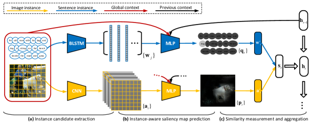
Figure 1: Details of the proposed sm-LSTM, including (a) instance candidate extraction, (b) instance-aware saliency map prediction, and (c) similarity measurement and aggregation (best viewed in colors).

3 Selective Multimodal LSTM

We will present the details of the proposed selective multimodal Long Short-Term Memory network (sm-LSTM) from the following three aspects: (a) instance candidate extraction for both image and sentence, (b) instance-aware saliency map prediction with a multimodal context-modulated attention scheme, and (c) local similarity measurement and aggregation with a multimodal LSTM.

3.1 Instance Candidate Extraction

Sentence Instance Candidates. For a sentence, its underlying instances mostly exist in word-level or phrase-level, e.g., dog and man. So we simply tokenlize and split the sentence into words, and then obtain their representations by sequentially processing them with a bidirectional LSTM (BLSTM) [27], where two sequences of hidden states with different directions (forward and backward) are learnt. We concatenate the vectors of two directional hidden states at the same timestep as the representation for the corresponding input word.

Image Instance Candidates. For an image, directly obtaining its instances is very difficult, since the visual content is unorganized where the instances could appear in any location with various scales. To avoid the use of additional object detectors, we evenly divide the image into regions as instance candidates as shown in Figure 1 (a), and represent them by extracting feature maps of the last convolutional layer in a CNN. We concatenate feature values at the same location across different feature maps as the feature vector for the corresponding convolved region.

3.2 Instance-aware Saliency Map Prediction

Apparently, neither the split words nor evenly divided regions can precisely describe the desired sentence or image instances. It is attributed to the fact that: 1) not all instance candidates are necessary since both image and sentence consist of too much instance-irrelevant information, and 2) the desired instances usually exist as a combination of multiple candidates, e.g., the instance dog covers about 12 image regions. Therefore, we have to evaluate the instance-aware saliency of each instance candidates, with the aim to highlight those important and ignore those irrelevant.

To achieve this goal, we propose a multimodal context-modulated attention scheme to predict pairwise instance-aware saliency maps for image and sentence. Different from [33], this attention scheme is designed for multimodal data rather than unimodal data, especially for the multimodal matching task. More importantly, we systematically study the importance of global context modulation in the attentional procedure. It results from an observation that each instance of image or sentence seldom occurs in isolation but co-varies with other ones as well as particular context. In particular, previous work [24] has shown that the global image scene enables humans to quickly guide their attention to regions of interest. A recent study [10] also demonstrates that the global sentence topic capturing long-range context can greatly facilitate inferring about the meaning of words.

As illustrated in Figure 1 (b), we denote the previously obtained instance candidates of image and sentence as $\left\{{{{\textbf{a}}_{i}}}|{{\textbf{a}}_{i}}\in{\mathbb{R}^{F}}\right\}_{i=1,\cdots,I}$ and $\left\{{{{\textbf{w}}_{j}}}|{{\textbf{w}}_{j}}\in{\mathbb{R}^{G}}\right\}_{j=1,\cdots,J}$, respectively. ${{\textbf{a}}_{i}}$ is the representation of the $i$-th divided region in the image and $I$ is the total number of regions. ${{\textbf{w}}_{j}}$ describes the $j$-th split word in the sentence and $J$ is the total number of words. $F$ is the number of feature maps in the last convolutional layer of CNN while $G$ is twice the dimension of hidden states in the BLSTM. We regard the output vector of the last fully-connected layer in the CNN as the global context $\textbf{m}\in{\mathbb{R}^{D}}$ for the image, and the hidden state at the last timestep in a sentence-based LSTM as the global context $\textbf{n}\in{\mathbb{R}^{E}}$ for the sentence. Based on these variables, we can perform instance-aware saliency map prediction at the $t$-th timestep as follows:

$${p_{t,i}}={{{e^{{{\hat{p}}_{t,i}}}}}}/{{\sum\nolimits_{i=1}^{I}{{e^{{{\hat{p}}_{t,i}}}}}}},{\kern 3.0pt}{{\hat{p}}_{t,i}}={f_{{p}}}(\textbf{m},{\textbf{a}_{i}},{{\textbf{h}}_{t-1}}),$$ (1)

$${q_{t,j}}={{{e^{{{\hat{q}}_{t,j}}}}}}/{{\sum\nolimits_{j=1}^{J}{{e^{{{\hat{q}}_{t,j}}}}}}},{\kern 3.0pt}{{\hat{q}}_{t,j}}={f_{{q}}}(\textbf{n},{\textbf{w}_{j}},{{\textbf{h}}_{t-1}})$$

where ${p_{t,i}}$ and ${q_{t,j}}$ are saliency values indicating probabilities that the $i$-th image instance candidate and the $j$-th sentence instance candidate will be attended to at the $t$-th timestep, respectively. $f_{{p}}(\cdot)$ and $f_{{q}}(\cdot)$ are two functions implementing the detailed context-modulation, where the input global context plays an essential role as reference information.

3.3 Global Context as Reference Information

To illustrate the details of the context-modulated attention, we take an image for example in Figure 2, the case for sentence is similar. The global feature m provides a statistical summary of the image scene, including semantic instances and their relationship with each other. Such a summary can not only provide reference information about expected instances, e.g., man and dog, but also cause the perception of one instance to generate strong expectations about other instances [5]. The local representations $\left\{{{{\textbf{a}}_{i}}}|{{\textbf{a}}_{i}}\in{\mathbb{R}^{F}}\right\}_{i=1,\cdots,I}$ describe all the divided regions independently and are used to compute the initial saliency map. The hidden state at the previous timestep ${\textbf{h}_{t-1}}$ indicates the already attended instances in the image, e.g., man.

To select which instance to attend to next, the attention scheme should first refer to the global context to find an instance, and then compare it with previous context to see if this instance has already been attended to. If yes (e.g., selecting the man), the scheme will refer to the global context again to find another instance. Otherwise (e.g., selecting the dog), regions in the initial saliency map corresponding to the instance will be highlighted. For efficient implementation, we simulate such a context-modulated attentional procedure using a simple three-way multilayer perceptrons (MLP) as follows:

$${f_{{p}}}(\textbf{m},{\textbf{a}_{i}},{{\textbf{h}}_{t-1}}) ={\kern 0.0pt}{\textbf{w}_{p}}(\sigma(\textbf{m}{W_{\textbf{m}}}+{\textbf{b}_{\textbf{m}}})+\sigma({\textbf{a}_{i}}{W_{\textbf{a}}}+{\textbf{b}_{\textbf{a}}})$$ (2)

$$+\sigma({\textbf{h}_{t-1}}{W_{\textbf{h}}}+{\textbf{b}_{\textbf{h}}}))+{{b}_{p}}$$

where $\sigma$ denotes the sigmoid activation function. ${\textbf{w}_{p}}$ and ${{b}_{p}}$ are a weight vector and a scalar bias. Note that in this equation, the information in initial saliency map is additively modulated by global context and subtractively modulated by previous context, to finally produce the instance-aware saliency map.

The attention schemes in [33, 2, 1] consider only previous context without global context at each timestep, they have to alternatively use step-wise labels serving as expected instance information to guide the attentional procedure. But such strong supervision can only be available for limited tasks, e.g., the sequential words of sentence for image caption [33], and multiple class labels for multi-object recognition [1]. For image and sentence matching, the words of sentence cannot be used as supervision information since we also have to select salient instances from the sentence to match image instances. In fact, we perform experiments without using global context in Section 4.7, but find that some instances like man and dog cannot be well attended to. It mainly results from the reason that without global context, the attention scheme can only refer to the initial saliency map to select which instance to attend to next, but the initial saliency map is computed from local representations that contain little instance information as well as relationship among instances.

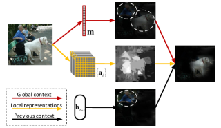
Figure 2: Illustration of context-modulated attention (the lighter areas indicate the attended instances, best viewed in colors).

3.4 Similarity Measurement and Aggregation

According to the predicted pairwise instance-aware saliency maps, we compute the weighted sum representations ${\textbf{a}^{\prime}_{t}}$ and ${\textbf{w}^{\prime}_{t}}$ to adaptively describe the attended image and sentence instances, respectively. We sum all the products of element-wise multiplication between each local representation (e.g., ${{\textbf{a}}_{i}}$) and its corresponding saliency value (e.g., ${p_{t,i}}$):

$${\textbf{a}^{\prime}_{t}}=\sum\nolimits_{i=1}^{I}{{p_{t,i}}{\textbf{a}_{i}}},{\kern 7.0pt}{\textbf{w}^{\prime}_{t}}=\sum\nolimits_{j=1}^{J}{{q_{t,j}}{\textbf{w}_{j}}}$$ (3)

where instance candidates with higher saliency values contribute more to the instance representations. Then, to measure the local similarity of the attended pairwise instances at the $t$-th timestep, we jointly feed their obtained representations ${\textbf{a}^{\prime}_{t}}$ and ${\textbf{w}^{\prime}_{t}}$ into a two-way MLP, and regard the output $\textbf{s}_{t}$ as the representation of the local similarity, as shown in Figure 1 (c).

From the 1-st to $T$-th timestep, we obtain a sequence of representations of local similarities $\left\{\textbf{s}_{t}\right\}_{t=1,\cdots,T}$, where $T$ is the total number of timesteps. To aggregate these local similarities for the global similarity, we use a LSTM network to sequentially take them as inputs, where the hidden states $\left\{\textbf{h}_{t}\in{\mathbb{R}^{H}}\right\}_{t=1,\cdots,T}$ dynamically propagate the captured local similarities until the end. The LSTM includes various gate mechanisms including memory state ${\textbf{c}_{t}}$, hidden state ${\textbf{h}_{t}}$, input gate $\textbf{i}_{t}$, forget gate $\textbf{f}_{t}$ and output gate $\textbf{o}_{t}$, which can well suit the complex nature of similarity aggregation:

$${\textbf{i}_{t}}=\sigma({W_{\textbf{s}\textbf{i}}}{\textbf{s}_{t}}+{W_{\textbf{h}\textbf{i}}}{\textbf{h}_{t-1}}+{\textbf{b}_{\textbf{i}}}),$$ (4)

$${\textbf{f}_{t}}=\sigma({{W}_{\textbf{s}\textbf{f}}}{\textbf{s}_{t}}+{W_{\textbf{h}\textbf{f}}}{\textbf{h}_{t-1}}+{\textbf{b}_{\textbf{f}}}),$$

$${\textbf{c}_{t}}={\textbf{f}_{t}}\odot{\textbf{c}_{t-1}}+{\textbf{i}_{t}}\odot\tanh({W_{\textbf{s}\textbf{c}}}{\textbf{s}_{t}}+{W_{\textbf{h}\textbf{c}}}{\textbf{h}_{t-1}}+{\textbf{b}_{\textbf{c}}}),$$

$${\textbf{o}_{t}}=\sigma({W_{\textbf{s}\textbf{o}}}{\textbf{s}_{t}}+{W_{\textbf{h}\textbf{o}}}{\textbf{h}_{t-1}}+{\textbf{b}_{\textbf{o}}}),{\textbf{h}_{t}}={\textbf{o}_{t}}\odot\tanh({\textbf{c}_{t}})$$

where $\odot$ denotes element-wise multiplication.

The hidden state at the last timestep ${\textbf{h}_{T}}$ can be regarded as the aggregated representation of all the local similarities. We use a MLP that takes ${\textbf{h}_{T}}$ as the input and produces the final matching score $s$ as global similarity:

$$s={\textbf{w}_{\textbf{h}s}}\left({\sigma\left({{{W}_{\textbf{hh}}}{\textbf{h}_{t}}+{\textbf{b}_{\textbf{h}}}}\right)}\right)+{b_{s}}.$$ (5)

3.5 Model Learning

The proposed sm-LSTM can be trained with a structured objective function that encourages the matching scores of matched images and sentences to be larger than those of mismatched ones:

$$\sum\nolimits_{ik}{{\max\left\{{0,m-s_{ii}+s_{ik}}\right\}}}+{{\max\left\{{0,m-s_{ii}+s_{ki}}\right\}}}$$ (6)

where $m$ is a tuning parameter, and $s_{ii}$ is the score of matched $i$-th image and $i$-th sentence. $s_{ik}$ is the score of mismatched $i$-th image and $k$-th sentence, and vice-versa with $s_{ki}$. We empirically set the total number of mismatched pairs for each matched pair as 100 in our experiments. Since all modules of our model including the extraction of local representations and global contexts can constitute a whole deep network, our model can be trained in an end-to-end manner from raw image and sentence to matching score, without pre-/post-processing. For efficient optimization, we fix the weights of CNN and use pretrained weights as stated in Section 4.2.

In addition, we add a pairwise doubly stochastic regularization to the objective, by constraining the sum of saliency values of any instance candidates at all timesteps to be 1:

$$\lambda\left(\sum\nolimits_{i}{({1-\sum\nolimits_{t}{{p_{t,i}}}})}+\sum\nolimits_{j}{({1-\sum\nolimits_{t}{{q_{t,j}}}})}\right)$$ (7)

where $\lambda$ is a balancing parameter. By adding this constraint, the loss will be large when our model attends to the same instance for multiple times. Therefore, it encourages the model to pay equal attention to every instance rather than a certain one for information maximization. In our experiments, we find that using this regularization can further improve the performance.

Table 1: Comparison results of image annotation and retrieval on the Flickr30K dataset. ($*$ indicates the ensemble or multi-model methods, and ^† indicates using external text corpora or manual annotations.)

Method	Image Annotation				Image Retrieval				Sum
	R$@$1	R$@$5	R$@$10	Med $r$	R$@$1	R$@$5	R$@$10	Med $r$
RVP (T+I) [4]	12.1	27.8	47.8	11	12.7	33.1	44.9	12.5	178.4
Deep Fragment [13]	14.2	37.7	51.3	10	10.2	30.8	44.2	14	188.4
DCCA [34]	16.7	39.3	52.9	8	12.6	31.0	43.0	15	195.5
NIC [31]	17.0	-	56.0	7	17.0	-	57.0	7	-
DVSA (BRNN) [14]	22.2	48.2	61.4	4.8	15.2	37.7	50.5	9.2	235.2
MNLM [15]	23.0	50.7	62.9	5	16.8	42.0	56.5	8	251.9
LRCN [7]	-	-	-	-	17.5	40.3	50.8	9	-
m-RNN [22]	35.4	63.8	73.7	3	22.8	50.7	63.1	5	309.5
FV†∗ [17]	35.0	62.0	73.8	3	25.0	52.7	66.0	5	314.5
m-CNN∗ [21]	33.6	64.1	74.9	3	26.2	56.3	69.6	4	324.7
RTP+FV†∗ [26]	37.4	63.1	74.3	-	26.0	56.0	69.3	-	326.1
RNN+FV† [19]	34.7	62.7	72.6	3	26.2	55.1	69.2	4	320.5
DSPE+FV† [32]	40.3	68.9	79.9	-	29.7	60.1	72.1	-	351.0
Ours:
sm-LSTM-mean	25.9	53.1	65.4	5	18.1	43.3	55.7	8	261.5
sm-LSTM-att	27.0	53.6	65.6	5	20.4	46.4	58.1	7	271.1
sm-LSTM-ctx	33.5	60.6	70.8	3	23.6	50.4	61.3	5	300.1
sm-LSTM	42.4	67.5	79.9	2	28.2	57.0	68.4	4	343.4
sm-LSTM∗	42.5	71.9	81.5	2	30.2	60.4	72.3	3	358.7

4 Experimental Results

To demonstrate the effectiveness of the proposed sm-LSTM, we perform experiments in terms of image annotation and retrieval on two publicly available datasets.

4.1 Datasets and Protocols

The two evaluation datasets and their corresponding experimental protocols are described as follows. 1) Flickr30k [35] consists of 31783 images collected from the Flickr website. Each image is accompanied with 5 human annotated sentences. We use the public training, validation and testing splits [15], which contain 28000, 1000 and 1000 images, respectively. 2) Microsoft COCO [20] consists of 82783 training and 40504 validation images, each of which is associated with 5 sentences. We use the public training, validation and testing splits [15], with 82783, 4000 and 1000 images, respectively.

4.2 Implementation Details

The commonly used evaluation criterions for image annotation and retrieval are “$\rm R@1$”, “$\rm R@5$” and “$\rm R@10$”, i.e., recall rates at the top 1, 5 and 10 results. Another one is “Med r” which is the median rank of the first ground truth result. We compute an additional criterion “Sum” to evaluate the overall performance for both image annotation and retrieval as follows:

$$\rm Sum=\underbrace{\rm R@1+\rm R@5+\rm R@10}_{Image{\kern 3.0pt}annotation}+\underbrace{\rm R@1+\rm R@5+\rm R@10}_{Image{\kern 3.0pt}retrieval}$$

To systematically validate the effectiveness, we experiment with five variants of sm-LSTMs: (1) sm-LSTM-mean does not use the attention scheme to obtain weighted sum representations for selected instances but instead directly uses mean vectors, (2) sm-LSTM-att only uses the attention scheme but does not exploit global context, (3) sm-LSTM-ctx does not use the attention scheme but only exploits global context, (4) sm-LSTM is our full model that uses both the attention scheme and global context, and (5) sm-LSTM^∗ is an ensemble of the described four models above, by summing their cross-modal similarity matrices together in a similar way as [21].

We use the 19-layer VGG network [28] to initialize our CNN to extract 512 feature maps (with a size of 14$\times$14) in “conv5-4” layer as representations for image instance candidates, and a feature vector in “fc7” layer as the image global context. We use MNLP [15] to initialize our sentence-based LSTM and regard the hidden state at the last timestep as the sentence global context, while our BLSTM for representing sentence candidates are directly learned from raw sentences with a dimension of hidden state as 512. For image, the dimensions of local and global context features are $F$=$512$ and $D$=$4096$, respectively, and the total number of local regions is $I$=$196$ (14$\times$14). For sentence, the dimensions of local and global context features are $G$=$1024$ and $E$=$1024$, respectively. We set the max length for all the sentences as 50, i.e., the number of split words $J$=$50$, and use zero-padding when a sentence is not long enough. Other parameters are empirically set as follows: $H$=$1024$, $\lambda$=$100$, $T$=$3$ and $m$=$0.2$.

Table 2: Comparison results of image annotation and retrieval on the Microsoft COCO dataset. ($*$ indicates the ensemble or multi-model methods, and ^† indicates using external text corpora or manual annotations.)

Method	Image Annotation				Image Retrieval				Sum
	R$@$1	R$@$5	R$@$10	Med $r$	R$@$1	R$@$5	R$@$10	Med $r$
STD†∗ [16]	33.8	67.7	82.1	3	25.9	60.0	74.6	4	344.1
m-RNN [22]	41.0	73.0	83.5	2	29.0	42.2	77.0	3	345.7
FV†∗ [17]	39.4	67.9	80.9	2	25.1	59.8	76.6	4	349.7
DVSA [14]	38.4	69.9	80.5	1	27.4	60.2	74.8	3	351.2
MNLM [15]	43.4	75.7	85.8	2	31.0	66.7	79.9	3	382.5
m-CNN∗ [21]	42.8	73.1	84.1	2	32.6	68.6	82.8	3	384.0
RNN+FV† [19]	40.8	71.9	83.2	2	29.6	64.8	80.5	3	370.8
OEM [30]	46.7	-	88.9	2	37.9	-	85.9	2	-
DSPE+FV† [32]	50.1	79.7	89.2	-	39.6	75.2	86.9	-	420.7
Ours:
sm-LSTM-mean	33.1	65.3	78.3	3	25.1	57.9	72.2	4	331.9
sm-LSTM-att	36.7	69.7	80.8	2	29.1	64.8	78.4	3	359.5
sm-LSTM-ctx	39.7	70.2	84.0	2	32.7	68.1	81.3	3	376.0
sm-LSTM	52.4	81.7	90.8	1	38.6	73.4	84.6	2	421.5
sm-LSTM∗	53.2	83.1	91.5	1	40.7	75.8	87.4	2	431.8

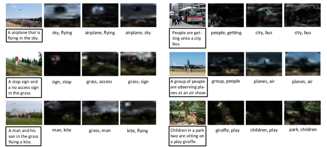
Figure 3: Visualization of attended image and sentence instances at three different timesteps (best viewed in colors).

4.3 Comparison with State-of-the-art Methods

We compare sm-LSTMs with several recent state-of-the-art methods on the Flickr30k and Microsoft COCO datasets in Tables 1 and 2, respectively. We can find that sm-LSTM^∗ can achieve much better performance than all the compared methods on both datasets. Our best single model sm-LSTM outperforms the state-of-the-art DSPE+FV^† in image annotation, but performs slightly worse than it in image retrieval. Different from DSPE+FV^† that uses external text corpora to learn discriminative sentence features, our model learns them directly from scratch in an end-to-end manner. Beside DSPE+FV^†, the sm-LSTM performs better than other compared methods by a large margin. These observations demonstrate that dynamically selecting image-sentence instances and aggregating their similarities is very effective for cross-modal retrieval.

When comparing among all the sm-LSTMs, we can conclude as follows. 1) Our attention scheme is effective, since sm-LSTM-att consistently outperforms sm-LSTM-mean on both datasets. When exploiting only context information without the attention scheme, sm-LSTM-ctx achieves much worse results than sm-LSTM. 2) Using global context to modulate the attentional procedure is very useful, since sm-LSTM greatly outperforms sm-LSTM-att with respect to all evaluation criterions. 3) The ensemble of four sm-LSTM variants as sm-LSTM^∗ can further improve the performance.

Table 3: The impact of different numbers of timesteps on the Flick30k dataset. $T$: the number of timesteps in the sm-LSTM.

	Image Annotation			Image Retrieval
	R$@$1	R$@$5	R$@$10	R$@$1	R$@$5	R$@$10
$T=1$	38.8	65.7	76.8	28.0	56.6	68.2
$T=2$	38.0	68.9	77.9	28.1	56.5	68.1
$T=3$	42.4	67.5	79.9	28.2	57.0	68.4
$T=4$	38.2	67.6	78.5	27.5	56.6	68.0
$T=5$	38.1	68.2	78.4	28.1	56.0	67.9

4.4 Analysis on Number of Timesteps

For a pair of image and sentence, we need to manually set the number of timesteps $T$ in sm-LSTM. Ideally, $T$ should be equal to the number of salient pairwise instances appearing in the image and sentence. Therefore, the sm-LSTM can separately attend to these pairwise instances within $T$ steps to measure all the local similarities. To investigate what is the optimal number of timesteps, in the following, we gradually increase $T$ from 1 to 5, and analyze the impact of different numbers of timesteps on the performance of sm-LSTM in Table 3.

From the table we can observe that sm-LSTM can achieve its best performance when the number of timesteps is 3. It indicates that it can capture all the local similarity information by iteratively visiting both image and sentence for 3 times. Intuitively, most pairs of images and sentences usually contain approximately 3 associated instances. Note that when $T$ becomes larger than 3, the performance slightly drops. It results from the fact that an overly complex network tends to overfit training data by paying attention to redundant instances at extra timesteps.

(a) Input image	(b) Without global context (by sm-LSTM-att)			(c) With global context (by sm-LSTM)

Figure 4: Attended image instances at three different timesteps, without or with global context, respectively (best viewed in colors).

Table 4: The impact of different values of the balancing parameter on the Flick30k dataset. $\lambda$: the balancing parameter between structured objective and regularization term.

	Image Annotation			Image Retrieval
	R$@$1	R$@$5	R$@$10	R$@$1	R$@$5	R$@$10
$\lambda=0$	37.9	65.8	77.7	27.2	55.4	67.6
$\lambda=1$	38.0	66.2	77.8	27.4	55.6	67.7
$\lambda=10$	38.4	67.4	77.7	27.5	56.1	67.6
$\lambda=100$	42.4	67.5	79.9	28.2	57.0	68.4
$\lambda=1000$	40.2	67.1	78.6	27.8	56.9	67.9

4.5 Evaluation of Regularization Term

In our experiments, we find that the proposed sm-LSTM is inclined to focus on the same instance at all timesteps, which might result from the fact that always selecting most informative instances can largely avoid errors. But it is not good for our model to comprehensively perceive the entire content in the image and sentence. So we add the pairwise doubly stochastic regularization term (in Equation 7) to the structured objective, with the aim to force the model to pay equal attention to all the potential instances at different locations. We vary the values of balancing parameter $\lambda$ from 0 to 1000, and compare the corresponding performance in Table 4. From the table, we can find that the performance improves when $\lambda$$>$$0$, which demonstrates the usefulness of paying attention to more instances. In addition, when $\lambda$$=$$100$, the ms-LSTM can achieve the largest performance improvement, especially for the task of image annotation.

4.6 Visualization of Instance-aware Saliency Maps

To verify whether the proposed model can selectively attend to salient pairwise instances of image and sentence at different timesteps, we visualize the predicted sequential instance-aware saliency maps by sm-LSTM, as shown in Figure 3. In particular for image, we resize the predicted saliency values at the $t$-th timestep ${\left\{{p_{t,i}}\right\}}$ to the same size as its corresponding original image, so that each value in the resized map measures the importance of an image pixel at the same location. We then perform element-wise multiplication between the resized saliency map and the original image to obtain the final saliency map, where lighter areas indicate attended instances. While for sentence, since different sentences have various lengths, we simply present two selected words at each timestep corresponding to the top-2 highest saliency values ${\left\{{q_{t,j}}\right\}}$.

We can see that sm-LSTM can attend to different regions and words at different timesteps in the images and sentences, respectively. Most attended pairs of regions and words describe similar semantic concepts. Taking the last pair of image and sentence for example, sm-LSTM sequentially focuses on words: “giraffe”, “children” and “park” at three different timesteps, as well as the corresponding image regions referring to similar meanings.

4.7 Usefulness of Global Context

To qualitatively validate the effectiveness of using global context, we compare the resulting instance-aware saliency maps of images generated by sm-LSTM-att and sm-LSTM in Figure 4. Without the aid of global context, sm-LSTM-att cannot produce accurate dynamical saliency maps as those of sm-LSTM. In particular, it cannot well attend to semantically meaningful instances such as “dog”, “cow” and “beach” in the first, second and third images, respectively. In addition, sm-LSTM-att always finishes attending to salient instances within the first two steps, and does not focus on meaningful instances at the third timestep any more. Different from it, sm-LSTM focuses on more salient instances at all three timesteps. These evidences show that global context modulation can be helpful for more accurate instance selection.

In Figure 5, we also compute the averaged saliency maps (rescaled to the same size of 500$\times$500) for all the test images at three different timesteps by sm-LSTM. We can see that the proposed sm-LSTM statistically tends to focus on the central regions at the first timestep, which is in consistent with the observation of “center-bias” in human visual attention studies [29, 3]. It is mainly attributed to the fact that salient instances mostly appear in the cental regions of images. Note that the model also attends to surrounding and lower regions at the other two timesteps, with the goal to find various instances at different locations.

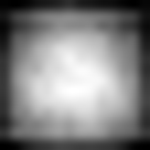
(a) 1-st timestep	(b) 2-nd timestep	(c) 3-rd timestep

Figure 5: Averaged saliency maps at three different timesteps.

5 Conclusions

In this paper, we have proposed the selective multimodal Long Short-Term Memory network (sm-LSTM) for instance-aware matching image and sentence. Our main contribution is proposing a multimodal context-modulated attention scheme to select salient pairwise instances from image and sentence, and a multimodal LSTM network for local similarity measurement and aggregation. We have systematically studied the global context modulation in the attentional procedure, and demonstrated its effectiveness with significant performance improvement. We have applied our model to the tasks of image annotation and retrieval, and achieved the state-of-the-art results. In the future, we will explore more advanced implementations of the context modulation (in Equation 2), and further verify our model on more datasets. We will also consider to jointly finetune the pretrained CNN for better performance.

References

- [1] J. Ba, V. Mnih, and K. Kavukcuoglu. Multiple object recognition with visual attention. In ICLR, 2015.
- [2] D. Bahdanau, K. Cho, and Y. Bengio. Neural machine translation by jointly learning to align and translate. In ICLR, 2014.
- [3] M. Bindemann. Scene and screen center bias early eye movements in scene viewing. Vision Research, 2010.
- [4] X. Chen and C. Lawrence Zitnick. Mind’s eye: A recurrent visual representation for image caption generation. In CVPR, 2015.
- [5] M. M. Chun and Y. Jiang. Top-down attentional guidance based on implicit learning of visual covariation. Psychological Science, 1999.
- [6] M.-C. De Marneffe, B. MacCartney, C. D. Manning, et al. Generating typed dependency parses from phrase structure parses. In LREC, 2006.
- [7] J. Donahue, L. Hendricks, S. Guadarrama, M. Rohrbach, S. Venugopalan, K. Saenko, and T. Darrell. Long-term recurrent convolutional networks for visual recognition and description. In CVPR, 2015.
- [8] H. Fang, S. Gupta, F. Iandola, R. K. Srivastava, L. Deng, P. Dollár, J. Gao, X. He, M. Mitchell, J. C. Platt, et al. From captions to visual concepts and back. In CVPR, 2015.
- [9] A. Frome, G. S. Corrado, J. Shlens, S. Bengio, J. Dean, T. Mikolov, et al. Devise: A deep visual-semantic embedding model. In NIPS, 2013.
- [10] S. Ghosh, O. Vinyals, B. Strope, S. Roy, T. Dean, and L. Heck. Contextual lstm (clstm) models for large scale nlp tasks. arXiv:1602.06291, 2016.
- [11] R. Girshick, J. Donahue, T. Darrell, and J. Malik. Rich feature hierarchies for accurate object detection and semantic segmentation. In CVPR, 2014.
- [12] S. Hochreiter and J. Schmidhuber. Long short-term memory. Neural Computation, 1997.
- [13] A. Karpathy, A. Joulin, and F.-F. Li. Deep fragment embeddings for bidirectional image sentence mapping. In NIPS, 2014.
- [14] A. Karpathy and F.-F. Li. Deep visual-semantic alignments for generating image descriptions. In CVPR, 2015.
- [15] R. Kiros, R. Salakhutdinov, and R. S. Zemel. Unifying visual-semantic embeddings with multimodal neural language models. TACL, 2015.
- [16] R. Kiros, Y. Zhu, R. R. Salakhutdinov, R. Zemel, R. Urtasun, A. Torralba, and S. Fidler. Skip-thought vectors. In NIPS, 2015.
- [17] B. Klein, G. Lev, G. Sadeh, and L. Wolf. Associating neural word embeddings with deep image representations using fisher vectors. In CVPR, 2015.
- [18] A. Krizhevsky, I. Sutskever, and G. E. Hinton. Imagenet classification with deep convolutional neural networks. In NIPS, 2012.
- [19] G. Lev, G. Sadeh, B. Klein, and L. Wolf. Rnn fisher vectors for action recognition and image annotation. In ECCV, 2016.
- [20] T.-Y. Lin, M. Maire, S. Belongie, J. Hays, P. Perona, D. Ramanan, P. Dollár, and C. L. Zitnick. Microsoft coco: Common objects in context. In ECCV. 2014.
- [21] L. Ma, Z. Lu, L. Shang, and H. Li. Multimodal convolutional neural networks for matching image and sentence. In ICCV, 2015.
- [22] J. Mao, W. Xu, Y. Yang, J. Wang, and A. L. Yuille. Explain images with multimodal recurrent neural networks. In ICLR, 2015.
- [23] T. Mikolov, K. Chen, G. Corrado, and J. Dean. Efficient estimation of word representations in vector space. In ICLR, 2013.
- [24] A. Oliva and A. Torralba. The role of context in object recognition. Trends in Cognitive Sciences, 2007.
- [25] F. Perronnin and C. Dance. Fisher kernels on visual vocabularies for image categorization. In CVPR, 2007.
- [26] B. Plummer, L. Wang, C. Cervantes, J. Caicedo, J. Hockenmaier, and S. Lazebnik. Flickr30k entities: Collecting region-to-phrase correspondences for richer image-to-sentence models. In ICCV, 2015.
- [27] M. Schuster and K. K. Paliwal. Bidirectional recurrent neural networks. IEEE Transactions on Signal Processing, 1997.
- [28] K. Simonyan and A. Zisserman. Very deep convolutional networks for large-scale image recognition. In ICLR, 2014.
- [29] P.-H. Tseng, R. Carmi, I. G. Cameron, D. P. Munoz, and L. Itti. Quantifying center bias of observers in free viewing of dynamic natural scenes. Journal of Vision, 2009.
- [30] I. Vendrov, R. Kiros, S. Fidler, and R. Urtasun. Order-embeddings of images and language. In ICLR, 2016.
- [31] O. Vinyals, A. Toshev, S. Bengio, and D. Erhan. Show and tell: A neural image caption generator. In CVPR, 2015.
- [32] L. Wang, Y. Li, and S. Lazebnik. Learning deep structure-preserving image-text embeddings. In CVPR, 2016.
- [33] K. Xu, J. Ba, R. Kiros, K. Cho, A. Courville, R. Salakhutdinov, R. S. Zemel, and Y. Bengio. Show, attend and tell: Neural image caption generation with visual attention. In ICML, 2016.
- [34] F. Yan and K. Mikolajczyk. Deep correlation for matching images and text. In CVPR, 2015.
- [35] P. Young, A. Lai, M. Hodosh, and J. Hockenmaier. From image descriptions to visual denotations: New similarity metrics for semantic inference over event descriptions. TACL, 2014.