The Thermal Proximity Effect: A new Probe of the He II Reionization History and the Quasar Lifetime

Abstract

Despite decades of effort, the timing and duration of He II reionization and the properties of the quasars believed to drive it, are still not well constrained. We present a new method to study both via the thermal proximity effect – the heating of the intergalactic medium (IGM) around quasars when their radiation doubly ionizes helium. We post-process hydrodynamical simulations with $1$D radiative transfer and study how the thermal proximity effect depends on He II fraction, $x_{\rm HeII,0}$, which prevailed in the IGM before the quasar turned on, and the quasar lifetime $t_{\rm Q}$. We find that the amplitude of the temperature boost in the quasar environment depends on $x_{\rm HeII,0}$, with a characteristic value of $\Delta T\simeq 10^{4}\,{\rm K}$ for $x_{\rm HeII,0}=1.0$, whereas the size of the thermal proximity zone is sensitive to $t_{\rm Q}$,with typical sizes of $\simeq 100\,{\rm cMpc}$ for $t_{\rm Q}=10^{8}\,{\rm yr}$. This temperature boost increases the thermal broadening of H I absorption lines near the quasar. We introduce a new Bayesian statistical method based on measuring the Ly$\alpha$ forest power spectrum as a function of distance from the quasar, and demonstrate that the thermal proximity effect should be easily detectable. For a mock dataset of $50$ quasars at $z\simeq 4$, we predict that one can measure $x_{\rm HeII,0}$ to an (absolute) precision $\approx 0.04$, and $t_{\rm Q}$ to a precision of $\approx 0.1$ dex. By applying our formalism to existing high-resolution Ly$\alpha$ forest spectra, one should be able to reconstruct the He II reionization history,providing a global census of hard photons in the high-$z$ universe.

1. Introduction

The Epoch of Reionization, when the intergalactic medium was ionized by astrophysical sources, is a key juncture in the history of the Universe. When and how reionization occurred informs models for the formation and evolution of the first stars, galaxies, and large-scale structure. Constraints on the Epoch of Reionization are derived mainly from the measurements of the Thompson scattering optical depth from the Cosmic Microwave Background (Robertson et al., 2015; Planck Collaboration et al., 2016) together with studies of the Ly$\alpha$ forest opacity towards high-redshift quasars (Fan et al., 2006; McGreer et al., 2011). It is widely believed that galaxies provide enough ionizing photons (Robertson et al., 2010; Finkelstein et al., 2012) to reionize intergalactic hydrogen by $z\simeq 6$. However, radiation from galaxies is unlikely to have been hard enough to have doubly ionized helium (He II $\longrightarrow$ He III, requiring $h\nu\geq 54.4$ eV). The current paradigm is that the complete reionization of helium was delayed until lower redshifts ($z\sim 3$), when quasars, which can emit the required energetic photons, became sufficiently abundant (Madau & Meiksin, 1994; Miralda-Escudé et al., 2000; McQuinn et al., 2009; Haardt & Madau, 2012; Compostella et al., 2013, 2014; La Plante et al., 2016).

The focus of this paper is on a new method to constrain this reionization of the last electron of helium, termed He II reionization. The temporal extent and morphology of He II reionization remains relatively unconstrained. Intergalactic He II Ly$\alpha$ absorption ($\lambda_{{\rm Ly}\alpha}^{\rm rest}=303.78{\rm\AA}$) in the far-UV spectra of $z_{\rm em}\simeq 3-4$ quasars directly probes He II in the IGM (Hogan et al., 1997; Anderson et al., 1999; Heap et al., 2000; Shull et al., 2010; Worseck et al., 2011; Syphers et al., 2012; Syphers & Shull, 2014; Worseck et al., 2014; Zheng et al., 2015). The recent discovery of regions in the IGM at $z\gtrsim 3.3$ with significant transmission (Worseck et al., 2011, 2014) suggests that He II reionization may have occurred earlier than current models predict (which generically reionize He II at the peak of the quasar epoch at $z\simeq 3$; McQuinn et al. 2009; Compostella et al. 2013, 2014; La Plante et al. 2016). However, this discrepancy could also result from uncertainties in the simulations and in simplistic models for quasar light curves (D’Aloisio et al., 2016).

If He II reionization did occur significantly earlier than current models predict, additional photons beyond those produced by $\gtrsim L_{*}$ quasars might be required. A possible candidate is a population of faint quasars (Giallongo et al., 2015; Madau & Haardt, 2015), but other exotic sources have also been proposed, including UV emission from $\sim 10^{6}$ K halos (Miniati et al., 2004), primordial globular clusters (Power et al., 2009), mini-quasars (Madau et al., 2004), and dark matter annihilations (Araya & Padilla, 2014). Irrespective of the nature of these sources, if they reionized intergalactic helium at $z\gtrsim 4$, these sources also likely contributed substantially to H I reionization (Madau & Haardt, 2015). Unfortunately, it is not currently possible to probe the ionization state of He II via far-UV He II Ly$\alpha$ absorption at $z\gtrsim 4$, and constraints on He II reionization from the thermal state of the IGM do not all agree (Lidz et al., 2010; Becker et al., 2011; Upton Sanderbeck et al., 2016). This paper introduces a new method to constrain the timing of He II reionization.

In the last decades significant effort was invested in measuring the thermal state of the IGM, aiming to constrain the timing of H I and He II reionization epochs. During these reionization events ionization fronts propagated supersonically impulsively heating IGM gas to $\sim 10^{4}~{}{\rm K}$, though the exact amount of injected heat depends on the spectral shape and abundance of the ionizing sources, and the opacity of the IGM (McQuinn, 2012; Davies et al., 2016). Hydrodynamical simulations show that within several hundred Myr of reionization, IGM gas relaxes onto a tight power law temperature-density relation $T=T_{0}(\rho/{\bar{\rho}})^{\gamma-1}$, where $T_{0}$ is the temperature at the cosmic mean density, $\bar{\rho}$ (Hui & Gnedin, 1997; McQuinn & Upton Sanderbeck, 2016). However, quasar driven He II reionization, which is thought to increase the temperature of the IGM by $\Delta T\simeq 5-10\times 10^{3}$ K at $z\simeq 3-4$ (McQuinn et al., 2009; Compostella et al., 2013), can lead to a significant changes in this relation (McQuinn et al., 2009; Upton Sanderbeck et al., 2016; La Plante et al., 2016). A comparable temperature increase at $z\simeq 3$ was reported by Schaye et al. (2000) (see also Theuns et al., 2002c), which was later qualitatively supported by Becker et al. (2011). However, there is generally a lack of consistency between these measurements and those from other studies (Ricotti et al., 2000; McDonald et al., 2001; Zaldarriaga et al., 2001; Lidz et al., 2010). In particular Lidz et al. (2010) found evidence for a much hotter IGM at $z\gtrsim 3.5$ than expected from current models (Puchwein et al., 2015; Upton Sanderbeck et al., 2016; Oñorbe et al., 2016), in disagreement with Becker et al. (2011).

Another important ingredient in reionization models is the quasar lifetime, which determines the morphology of the hard UV background (McQuinn et al., 2009; Compostella et al., 2013, 2014; McQuinn & Worseck, 2014). Recent lifetime estimates based on the light travel time arguments in quasar host galaxies ($t_{\rm Q}\simeq 10^{5}$ yr; Schawinski et al., 2010, 2015), and quasar powered Ly$\alpha$ fluorescence ($10^{6}\lesssim t_{\rm Q}\lesssim 3\times 10^{7}$ yr; Trainor & Steidel, 2013; Borisova et al., 2015) are indirect, and alternative physical mechanisms can be invoked to explain the observations. To date the most robust estimates of the quasar lifetime are derived from the line-of-sight H I proximity effect (Bajtlik et al., 1988; Haiman & Cen, 2002) in Ly$\alpha$ forest spectra. The quasar must shine for $t_{\rm Q}\gtrsim t_{\rm eq}$ to produce a detectable proximity zone, where the equilibration timescale $t_{\rm eq}\simeq\Gamma_{\rm HI}^{-1}$ is the time it takes for the IGM to reach ionization equilibrium with the quasar radiation. At $z\simeq 3-5$, the H I photoionization rate is constrained to be $\Gamma_{\rm HI}\simeq 10^{-12}{\rm s^{-1}}$, which means light curve variations from the proximate quasar will only produce a line-of-sight proximity effect if $t_{\rm Q}\gtrsim 3\times 10^{4}$ yr. On a positive note, Khrykin et al. (2016) demonstrated that He II Ly$\alpha$ line-of-sight proximity zones in the far-UV spectra of $z\simeq 3-4$ can probe quasar lifetimes on the more interesting timescale of $\sim 10$ Myr, although this method has yet to be applied to real data. Here we propose another method that we show is sensitive to comparable lifetimes based on H I Ly$\alpha$ spectra, for which there exists a substantial amount of high-${\rm S/N}$, high-resolution data.

Before reionization is complete, quasars that turn on in a medium in which the helium is initially He II, doubly ionize it, creating He III regions. Photoionization of He II $\longrightarrow$ He III produces suprathermal photoelectrons, which are thermalized, raising the temperature of the gas by $\sim 10^{4}$K (Abel & Haehnelt, 1999; Miralda-Escudé & Rees, 1994; McQuinn et al., 2009; Bolton et al., 2009). Such an increase in IGM temperatures in the quasar environs is referred to as the thermal proximity effect. As discussed by Bolton et al. (2009) and Meiksin et al. (2010), this temperature boost due to the evolution of He II fraction can significantly alter the H I Ly$\alpha$ forest around the quasar via additional thermal broadening of the Ly$\alpha$ absorption lines. For instance, Bolton et al. (2010, 2012) claimed to measure IGM temperatures $\simeq 0.3$ dex higher than expected in the proximity zones of $z\sim 6$ quasars, attributing this extra heating to the quasar reionizing its surrounding He II. They also showed that this temperature boost can be used to infer the quasar lifetime, and estimated a lower limit $t_{\rm Q}\gtrsim 10^{6.5}$ yr.

The aim of this paper is to further investigate the line-of-sight thermal proximity effect, quantify its detectability, and determine how well it can constrain the timing of He II reionization and the average quasar lifetime. We combine cosmological hydrodynamical simulations with post-processing radiative transfer calculations using the $1$D radiative transfer algorithm specifically developed in Khrykin et al. (2016) for this purpose, which allows us to track the changes in the ionization state of helium and hydrogen, and the associated temperature of the IGM around quasars. We apply the power spectrum statistic to the output of our simulations, which is directly sensitive to thermal broadening, and thus to the average temperature profile around quasars. We use Bayesian methods with Markov Chain Monte Carlo (MCMC) calculations to determine the accuracy with which the amount of singly ionized helium in the IGM and the quasar lifetime can be determined.

This paper is organized as follows. In § 2 we briefly explore the most important parameters of our numerical model. We describe the thermal proximity effect during He II reionization and show its impact on the properties of the IGM gas in § 3. We introduce our method for measuring He II fraction and quasar lifetime from the $1$D Ly$\alpha$ forest power spectrum in § 4. We present the results of our MCMC analysis in § 5, and explore the possibility of reconstructing the history He II reionization in § 6. We briefly explore wavelet analysis as another method to detect the thermal proximity effect in § 7. Possible uncertainties and systematic errors are discussed in § 8, and we summarize and conclude in § 9.

Throughout this paper we assume a flat $\Lambda$CDM cosmology with Hubble constant $h=0.7$, $\Omega_{\rm m}=0.27$, $\Omega_{\rm b}=0.046$, $\sigma_{8}=0.8$ and $n_{s}=0.96$, and helium mass fraction $Y_{\rm He}=0.24$, consistent with recent Planck results (Planck Collaboration et al., 2016). All distances are quoted in units of comoving Mpc, i.e., cMpc.

As noted above, one of the goals of this paper is to understand the constraints that can be put on the quasar lifetime, which is the time spanned by a single episode of accretion onto the black hole. One should distinguish this from the quasar duty cycle, which refers to the total time that galaxies shine as active quasars. In the context of proximity effects in the IGM, one actually only constrains the quasar on-time, which we will denote as $t_{\rm Q}$. If we imagine that time $t=0$ corresponds to the time when the quasar emitted light that is just now reaching our telescopes on Earth, then the quasar on-time is defined such that the quasar turned on at time $-t_{\rm Q}$ in the past. This timescale is, in fact, a lower limit on the quasar lifetime, which arises from the fact that we observe a proximity zone at $t=0$ when the quasar has been shining for time $t_{\rm Q}$, whereas this quasar episode may indeed continue, which we can only record on Earth if we could conduct observations in the future. For simplicity in the text, we will henceforth refer to the quasar on-time as the quasar lifetime denoted by $t_{\rm Q}$, but the reader should always bear in mind that this is actually a lower limit on the duration of quasar emission episodes.

2. Summary of the Numerical model

We use a combination of smooth particle hydrodynamics (SPH) simulations and a $1$D post-processing radiative transfer algorithm to study the thermal evolution of the intergalactic medium around quasars. In this section we present the most important features of our model and refer the reader to the more detailed description given in Khrykin et al. (2016).

2.1. Hydrodynamical Simulations

We run SPH simulations using the Tree-SPH code Gadget-3 (Springel, 2005) with $2\times 512^{3}$ particles and a box size of $25h^{-1}$ cMpc. Starting at the location of the most massive halos (${\rm M}>5\times 10^{11}{\rm M}_{\odot}$) at $z=\left[3.1,3.5,3.9,4.3,4.6\right]$ we extract $1000$ sightlines (which we will refer to as skewers) by casting the rays through the simulation box at random angles and using the periodic boundary conditions to wrap the skewers through the simulation volume. The resulting skewers have a total length of $160$ cMpc with a pixel scale of ${\rm d}r=0.01$ cMpc (${\rm d}v=1.0\ {\rm km\ s^{-1}}$). While most of the discussion in this paper focuses on the output at $z=3.9$, we consider other redshifts as well in § 6. Note that we also perform our calculations at redshift $z=5.0$, for which we do not have outputs of the hydrodynamical simulations. However, assuming that there is no evolution of the density field between two redshifts, and the only change is due to the cosmological expansion, we simply re-scaled the density field of $z=4.6$ output by a factor of $\left(1+z\right)^{3}$, which is a good approximation.

2.2. Radiative Transfer Algorithm

Skewers are extracted from the SPH simulation volume, and are post-processed using our $1$D radiative transfer algorithm, based on the C²-Ray algorithm (Mellema et al., 2006). We assume the quasar, placed at the beginning of each skewer, has a spectral energy distribution (SED) which can be approximated by a power-law, such that its specific photon production rate $N_{\nu}$ at frequencies $\nu\geq\nu_{\rm th}$ is given by

$$N_{\nu}=\frac{\alpha Q}{\rm\nu_{th}}\left(\frac{\rm\nu}{\nu_{\rm th}}\right)^{-\left(\alpha+1\right)},$$ (1)

where $Q$ is the production rate (${\rm photons}\ {\rm s}^{-1}$) of photons with frequency above the H I (or He II) ionization threshold $\nu_{\rm th}$, and the spectral index is assumed to be $\alpha=1.5$ ($f_{\nu}\sim\nu^{-\alpha}$), consistent with inferred values from UV composite quasar spectra (Telfer et al., 2002; Shull et al., 2012; Lusso et al., 2015). Following the procedure described in Hennawi et al. (2006) (see also Khrykin et al. (2016) for details), we find that for a median $i$-band magnitude $i=18.6$ of quasars at $z\simeq 4$ the $Q_{\rm 1Ry}\simeq 10^{57.4}{\rm s^{-1}}$ and $Q_{\rm 4Ry}\simeq 10^{56.5}{\rm s^{-1}}$, which we adopt as our fiducial values throughout the paper.

2.2.1 Photoionization of He II

The quasar He II photoionization rate in each cell is given by

$$\Gamma_{\rm HeII}^{\rm QSO}=\int_{\nu_{\rm 4Ry}}^{\infty}\frac{N_{\rm\nu}e^{-\langle\tau_{\rm\nu}\rangle}\left(1-e^{-\langle\delta\tau_{\rm\nu}\rangle}\right)}{\langle n_{\rm HeII}\rangle V_{\rm cell}}d\nu,$$ (2)

where $\langle\tau_{\nu}\rangle$ is the optical depth along the skewer from the source to the current cell, $\langle\delta\tau_{\nu}\rangle$ is the optical depth inside the cell, $\langle n_{\rm HeII}\rangle$ is the average number density of He II in this cell, and $V_{\rm cell}$ is the volume of the cell. The angular brackets indicate time averages over the discrete time step $\delta t$. Combining with eqn. (1), eqn. (2) becomes:

$$\small\Gamma_{\rm HeII}^{\rm QSO}=\frac{\alpha Q_{\rm 4Ry}}{n_{\rm HeII}V_{\rm cell}\nu_{\rm th}}\int_{\nu_{\rm th}}^{\infty}\left(\frac{\nu}{\nu_{\rm th}}\right)^{-(\alpha+1)}e^{-\langle\tau_{\rm\nu}\rangle}\left(1-e^{-\langle\delta\tau_{\nu}\rangle}\right)d\nu.$$ (3)

We note that our radiative transfer algorithm is not tracking multiple frequencies, but rather calculates the frequency-integrated quasar photoionization rate given by eqn (3). For a given quasar SED (eqn. 1), and approximating the He II absorption cross-section as $\sigma_{\nu}\approx\sigma_{\rm th}\left(\nu/\nu_{\rm th}\right)^{-3}$, eqn. (3) has a direct analytic solution depending on $\langle\tau_{\rm th}\rangle$ and $\langle\delta\tau_{\rm th}\rangle$, evaluated at a single frequency corresponding to the He II $4$ Ry ionization threshold.

In order to account for additional ionizations caused by He II ionizing photons emitted by other sources in the Universe, we also include the He II intergalactic ionizing background in our calculations. We approximate it as being constant in space and time, and we add it in each pixel of our skewers, yielding the total He II photoionization rate $\Gamma_{\rm HeII}^{\rm tot}=\Gamma_{\rm HeII}^{\rm QSO}+\Gamma_{\rm HeII}^{\rm bkg}$. We also include a prescription for more careful modeling of the attenuation of He II ionizing background by He II-LLSs (McQuinn & Switzer, 2010), details of which can be found in Appendix B of Khrykin et al. (2016).

2.2.2 Time-evolution of He II Fraction

Given eqn. (3), the time-evolution of the He II fraction $x_{\rm HeII}\left(t\right)$ is described by

$$\frac{dx_{\rm HeII}}{dt}=-\Gamma_{\rm HeII}^{\rm tot}\left(t\right)\,x_{\rm HeII}+n_{\rm e}\alpha_{\rm A}^{\left[{\rm HeII}\right]}\left(1-x_{\rm HeII}\right),$$ (4)

where $n_{\rm e}$ is the number density of free electrons, and $\alpha_{\rm A}^{\left[{\rm HeII}\right]}$ is the He II Case A recombination coefficient. In Khrykin et al. (2016) we showed that evolution of He II proximity zones around quasars can be described by the He II fraction $x_{\rm HeII}$ approaching ionization equilibrium. This approach depends on the characteristic timescale on which the He II ionization state of IGM gas responds to the changes in the radiation field, i.e., the equilibration time, given by

$$t_{\rm eq}=\left(\Gamma_{\rm HeII}^{\rm tot}+n_{\rm e}\alpha_{\rm A}^{\left[{\rm HeII}\right]}\right)^{-1}\approx\Gamma_{\rm HeII}^{\rm tot}\ {}^{-1}$$ (5)

Since for He II at $z\simeq 3-4$ the equilibration timescale is $t_{\rm eq}^{\rm\left[HeII\right]}\approx 10^{7}$ yr, comparable to quasar lifetimes $t_{\rm Q}$, the ionization equilibrium is a poor approximation. Hence, we follow the full time-dependent radiative transfer of He II in the proximity zone.

The mean initial He II fraction $x_{\rm HeII,0}$ is calculated from $100$ skewers by running our radiative transfer algorithm with quasar turned off, and the He II background being the only source of ionizations. The desired value of $x_{\rm HeII,0}$ is then set by adjusting the He II ionizing background. These He II background values are then used in radiative transfer calculations with quasar turned on.

Further, using our $1$D radiative transfer algorithm we integrate eqn. (4) for the time-evolution of $x_{\rm HeII}$ over time $t=t_{\rm Q}$, which denotes the quasar lifetime, yielding the He II fraction $x_{\rm HeII}$ at each location along the given skewer. We refer the interested reader to Khrykin et al. (2016) for more detailed description of our radiative transfer calculations, the time-evolution of He II fraction, and its effect on the structure of the quasar proximity zones.

2.2.3 Treatment of H I

Analogous to eqn. (2), our radiative transfer algorithm calculates the quasar H I photoionization rate $\Gamma_{\rm HI}^{\rm QSO}$ given by

$$\Gamma_{\rm QSO}^{\rm HI}=\frac{1}{4\pi r^{2}}\int_{\nu_{\rm 1Ry}}^{\infty}N_{\nu}\sigma_{\rm HI}{\rm d}\nu,$$ (6)

where $\sigma_{\rm HI}$ is H I absorption cross-section, and we assumed that hydrogen is highly ionized and hence optically thin to ionizing radiation, which is valid at $z\lesssim 6$, well after H I reionization has been completed. We also assume that all radiation at frequencies $\nu\gtrsim\nu_{4{\rm Ry}}$ is absorbed by He II, which is valid for the same case of highly ionized H I.

Similar to helium, we introduce the metagalactic H I ionizing background, described by the photoionization rate $\Gamma_{\rm HI}^{\rm bkg}$, to quantify the influence of all other sources of H I ionizing photons, i.e., $\Gamma_{\rm HI}^{\rm tot}=\Gamma_{\rm HI}^{\rm QSO}+\Gamma_{\rm HI}^{\rm bkg}$. The value of $\Gamma_{\rm HI}^{\rm bkg}$ is chosen to match the mean transmission at all redshifts considered in this work, consistent with the measurements of Becker et al. (2013a)

Because the H I equlibration time is so short, i.e. $t_{\rm eq}^{\rm\left[HI\right]}\sim\Gamma_{\rm HI}^{-1}\approx 10^{4}$ yr, we assume that H I is in ionization equilibrium, which is an excellent approximation provided $t_{\rm Q}\gg\Gamma_{\rm HI}^{-1}$. Hence, under this assumption, the H I fraction $x_{\rm HI}$ at every pixel along the skewer is set by

$$x_{\rm HI}=n_{\rm e}\alpha_{\rm A}^{\left[{\rm HI}\right]}\left(n_{\rm e}\alpha_{\rm A}^{\left[{\rm HI}\right]}+\Gamma_{\rm HI}^{\rm tot}\right)^{-1},$$ (7)

where $\alpha_{\rm A}^{\left[{\rm HI}\right]}$ is the H I Case A recombination coefficient. We note that in our radiative transfer calculations we have assumed that all neutral helium, i.e., He I, has been already singly ionized together with H I at $z\gtrsim 6$. Hence, the He I fraction is $x_{\rm HeI}\ll 1$. Therefore, the He I electrons are taken into account when computing the fractions of He II and H I, whereas He II electrons are used according to the computed $x_{\rm HeII}$ from the radiative transfer algorithm.

2.3. Evolution of the Temperature

Consider an element of ideal gas in the expanding Universe exposed to the quasar radiation. The temperature $T$ of the gas element then evolves with time $t$ according to the first law of thermodynamics (see Hui & Gnedin, 1997)

$$\frac{{\rm d}T}{{\rm d}t}=-2HT+\frac{2T}{3\left(1+\delta\right)}\frac{{\rm d}\delta}{{\rm d}t}-\frac{T}{\Sigma_{i}X_{i}}\frac{{\rm d}\Sigma_{i}X_{i}}{{\rm d}t}+\frac{2}{3k_{\rm B}n_{\rm b}}\frac{{\rm d}E}{{\rm d}t},$$ (8)

where $H$ is the Hubble parameter, $E$ is the internal energy of the gas, $n_{\rm b}$ is the number density of the baryonic particles (including electrons), and $k_{\rm B}$ is the Boltzmann constant.

The first term on the right-hand side of eqn. (8) corresponds to adiabatic cooling due to the expansion of the Universe. The expansion cooling timescale of the low density photoionized gas in the IGM ($\Delta\lesssim 10$) is the Hubble time $t_{\rm H}$ (Miralda-Escudé & Rees, 1994). Thus, because $t_{\rm H}\left(z\simeq 4\right)\sim 2\times 10^{9}$ yr is much longer than the quasar lifetimes we consider in this paper ($10^{6}\ {\rm yr}\leq t_{\rm Q}\leq 10^{8}\ {\rm yr}$), this term would result in a small change in the temperature of the gas over this timescale and therefore is neglected in our analysis. The second term describes the cooling or heating from structure formation, which also has a characteristic time of the Hubble time, $t_{\rm H}$. Thus, this term can be neglected for the same reason as the first one, i.e. $t_{\rm Q}/t_{\rm H}\ll 1$. The third term, which represents the change in the internal energy of the gas particles due to the change in the number of particles is also smaller than the dominant heating mechanism during reionization described by the last term ($\approx 4\%$; Upton Sanderbeck et al., 2016), which accounts for the amount of heat gained (lost) per unit volume from radiation processes. Hence, assuming that hydrogen is already ionized and helium is singly ionized (He I $\longrightarrow$ He II), and that gas is exposed to the quasar radiation for the time $t_{\rm Q}\ll t_{\rm H}$, we can simplify eqn. (8) to

$$\frac{{\rm d}T}{{\rm d}t}\simeq\frac{2}{3k_{\rm B}n_{\rm b}}\frac{{\rm d}E}{{\rm d}t}=\frac{2}{3k_{\rm B}n_{\rm b}}n_{\rm HeII}\epsilon_{\rm HeII},$$ (9)

where $n_{\rm HeII}$ is the number density of He II atoms and $\epsilon_{\rm HeII}$ is the total quasar photoheating rate. Using eqn. (4) and given that the recombination timescale is very long compared to the photoionization timescale ($t_{\rm rec}\simeq 10^{9}~{}{\rm yr}\gg 1/\Gamma^{\rm tot}_{\rm HeII}$), and ignoring collisional ionization of He II, the rate of change of He II number density $n_{\rm HeII}$ is

$$\frac{{\rm d}n_{\rm HeII}}{{\rm d}t}=-n_{\rm HeII}\Gamma_{\rm HeII}^{\rm tot}$$ (10)

Therefore, combining eqn. (9) and eqn. (10) yields

$$\frac{{\rm d}T}{{\rm d}t}\simeq\frac{2}{3k_{\rm B}n_{\rm b}}\biggl{|}\frac{{\rm d}n_{\rm HeII}}{{\rm d}t}\biggr{|}\frac{\epsilon_{\rm HeII}}{\Gamma_{\rm HeII}^{\rm tot}}.$$ (11)

We can also write ${\rm d}n_{\rm HeII}/{\rm dt}$ in terms of He II fraction $x_{\rm HeII}$ as

$$\frac{{\rm d}n_{\rm HeII}}{{\rm d}t}=\frac{\rho_{\rm crit}\Omega_{\rm b}}{m_{\rm p}}\frac{Y_{\rm He}}{4}\left(1+\delta\right)\left(1+z\right)^{3}\frac{{\rm d}x_{\rm HeII}}{{\rm d}t},$$ (12)

where $\rho_{\rm crit}$ is the critical density of the Universe, $m_{\rm p}$ is the mass of proton, and $\left(1+\delta\right)$ is the gas density in units of the cosmic mean density. Finally, combining eqn. (11) and eqn. (12) and taking into account that the total number density of baryons is $n_{b}\approx n_{\rm H}+n_{\rm He}+n_{\rm e}$ (number density of hydrogen and helium atoms, and electrons) the temperature evolution is given by

$$\frac{{\rm d}T}{{\rm d}t}\simeq\frac{2}{3k_{\rm B}}\frac{Y_{\rm He}}{4\left(2-5Y_{\rm He}/4\right)}\frac{{\rm d}x_{\rm HeII}}{{\rm d}t}\langle E\rangle$$ (13)

where $\langle E\rangle=\epsilon_{\rm HeII}/\Gamma_{\rm HeII}^{\rm tot}$ is the average excess energy per per photoionization of a He II atom given by

$$\langle E\rangle=\Bigg{[}\int_{\nu_{\rm th}}^{\infty}N_{\nu}\sigma_{\nu}e^{-\langle\tau_{\rm\nu}\rangle}\left(1-e^{-\langle\delta\tau_{\nu}\rangle}\right)\left(h\nu-h\nu_{\rm th}\right) {\rm d}\nu\Bigg{]}$$

$$\Bigg{/}\Bigg{[}\int_{\nu_{\rm th}}^{\infty}N_{\nu}\sigma_{\nu}e^{-\langle\tau_{\rm\nu}\rangle}\left(1-e^{-\langle\delta\tau_{\nu}\rangle}\right){\rm d}\nu\Bigg{]}$$ (14)

We neglect the heating by the H I and He II ionizing background, since this is accounted for via the treatment of photoionization heating in the hydrodynamical simulation. Given the quasar SED slope $\alpha$ (eqn. 1), the frequency integral for the the average excess energy per ionization $\langle E\rangle$ in eqn. (2.3) has an analytical solution, which is then evaluated at each time step of our $1$D radiative transfer calculations using the values of $\langle\tau_{\nu}\rangle$ and $\langle\delta\tau_{\nu}\rangle$ computed by the code. If we assume an optically thin limit and use eqn. (13), we can estimate the lower limit on expected heating produced by the quasar $\Delta T\simeq 0.6h\nu_{\rm th}/[28\ k_{\rm B}\left(\alpha+2\right)]\simeq 4500^{\circ}{\rm K}$ (McQuinn et al., 2009). In reality, however, the exact amount of heating depends on how many of hard photons are absorbed close to the quasar (i.e., their mean-free path), the properties of quasar itself and the history of He II reionization.

2.4. Examples Outputs from the Radiative Transfer Code

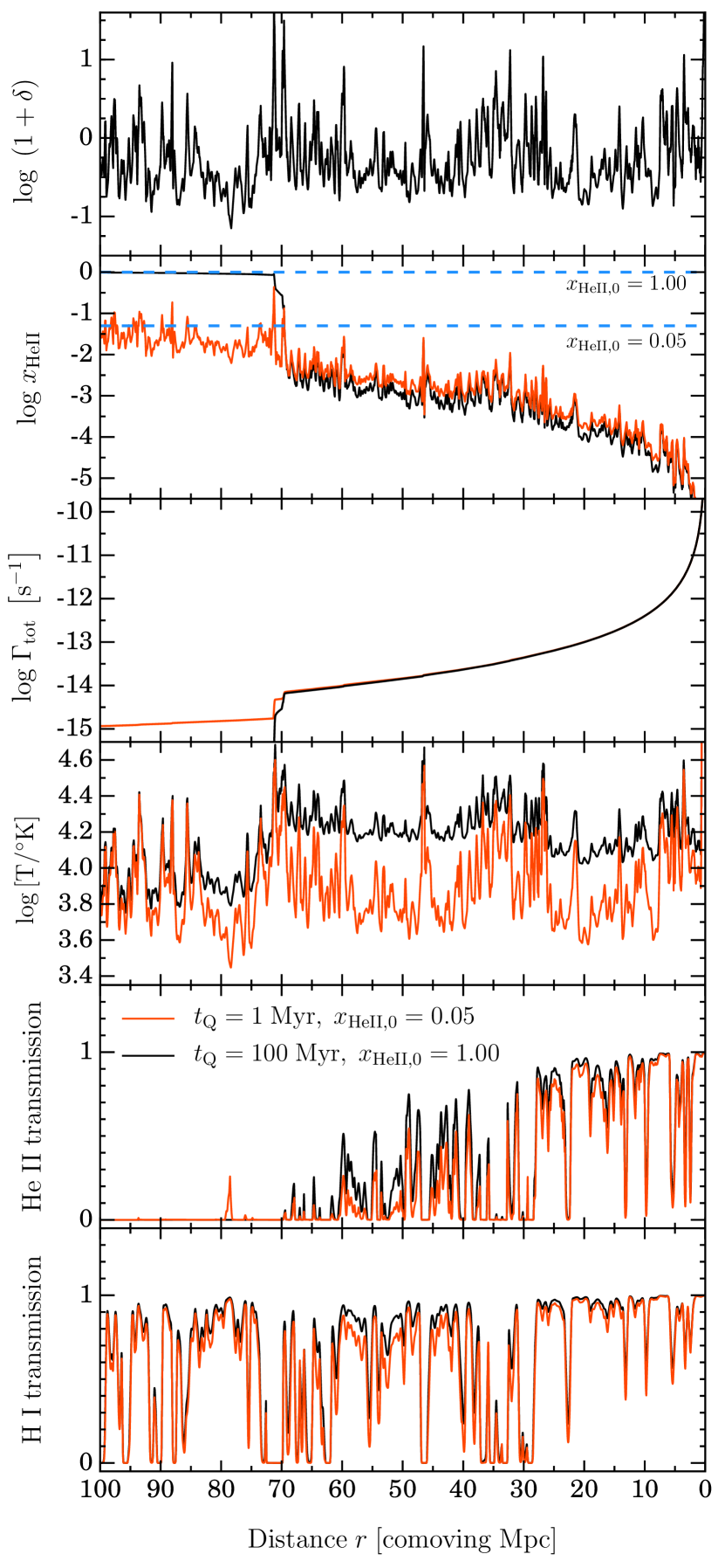
Figure 1.— Example sightline at $z=3.9$ from our radiative transfer calculations assuming a quasar turns on for $t_{\rm Q}=10^{6}$ yr in IGM with initial He II fraction $x_{\rm HeII,0}=0.05$ (red) and $t_{\rm Q}=10^{8}$ yr in IGM with $x_{\rm HeII,0}=1.00$ (black). We indicate the initial He II fractions $x_{\rm HeII,0}$ before the quasar is on by the dashed lines in the panel with $x_{\rm HeII}$ evolution. The x-axis indicates distance $r$ from the quasar in units of comoving Mpc. Panels show (from top to bottom): the overdensity, the He II fraction $x_{\rm HeII}$, the He II photoionization rate $\Gamma_{\rm HeII}^{\rm tot}$, the temperature of the gas $T$, transmission in He II and H I, respectively.

Following the approach described in Theuns et al. (1998), we calculate H I and He II spectra along each of the skewers taken from the SPH simulations at all considered redshifts. Figure 1 illustrates an example output of our radiative transfer calculations with multiple physical quantities along one skewer. The quasar is located at $r=0$. We show results from two models: the red curves assume a quasar which shines for $t_{\rm Q}=10^{6}$ yr in an IGM where helium is already largely doubly ionized with $x_{\rm HeII,0}=0.05$, where $x_{\rm HeII,0}$ represents the He II fraction before the quasar turns on. Whereas for the black curves the quasar shines for a longer $t_{\rm Q}=10^{8}$ yr in an initially singly ionized IGM (i.e. before the epoch of He II reionization) with $x_{\rm HeII,0}=1.0$. The quasar photon production rates at H I and He II ionization thresholds are set to our fiducial values (see Section 2.2).

The uppermost panel of Figure 1 plots the gas density along the skewer in units of the cosmic mean density. The second panel from the top illustrates the He II fraction for the two models. The horizontal dashed lines indicate the initial He II fraction set by He II ionizing background only, which prevailed in the IGM prior to the quasar turning on (see § 2.2.2). As expected, close to the quasar (at $r\lesssim 20$ cMpc) helium is highly doubly ionized ($x_{\rm HeII,0}\lesssim 10^{-3.5}$) in both models due to the quasar’s radiation. However, because the quasar photoionization rate drops off approximately as $r^{-2}$, which is illustrated in the third panel from the top, at larger radii it becomes sufficiently small and no longer dominates over the He II background. Therefore, the $x_{\rm HeII}$ in both models asymptote to the initial values set by $\Gamma_{\rm HeII}^{\rm bkg}$, i.e., $x_{\rm HeII,0}=0.05$ (red) and $x_{\rm HeII,0}=1.00$ (black), respectively.

The fourth panel from the top illustrates the IGM temperature along the skewer. According to eqn. (13) the heat input due to quasar radiation is proportional to the change in the He II fraction as the quasar ionization front traverses through the surrounding IGM. Hence, the temperature in the $x_{\rm HeII,0}=1.00$ model, where the quasar radiation significantly changes $x_{\rm HeII}$, is $\approx 2$ times higher, than that of the $x_{\rm HeII,0}=0.05$ model, in which the IGM was already highly doubly ionized to begin with.

As expected, the He II transmission (fourth panel from the top), which depends on $x_{\rm HeII}$, follows the general radial trend set by the evolution of the He II fraction. It is apparent from Figure 1 that, the sizes of He II proximity zones in two illustrated models are nearly identical, despite the different values of $t_{\rm Q}$ and $\Gamma_{\rm HeII}^{\rm bkg}$ used in these models. Indeed, as we showed in Khrykin et al. (2016), there is a significant degeneracy between $x_{\rm HeII}$ and quasar lifetime $t_{\rm Q}$ in setting the sizes of He II Ly$\alpha$ proximity zones. Remember that acquiring far ultraviolet He II Ly$\alpha$ spectra of quasars at such high redshifts ($z\gtrsim 3.9$) is extremely difficult, therefore, it will be hard to break this degeneracy and determine $t_{\rm Q}$ and $x_{\rm HeII}$ directly from the spectra. The apparent difference in IGM temperatures in two considered models is also difficult to distinguish from the effect of this degeneracy.

The H I transmission, on the other hand, which can be directly probed with optical spectra to much higher redshifts $z\lesssim 6$, when hydrogen is highly ionized after the end of H I reionization, is also sensitive to the heating of the intergalactic gas. The bottom panel of Figure 1 shows that H I Ly$\alpha$ transmission in the hotter model (black curve) with $x_{\rm HeII,0}=1.00$ is smoother and shows less small-scale structure, than that of cooler $x_{\rm HeII,0}=0.05$ model. This so-called “thermal proximity effect” due to the nearby quasar radiation results from thermal Doppler broadening and the differences in IGM temperature between the two models (see middle panel of Figure 1). In § 4 we show that this effect can be used to constrain the parameters of interest, i.e., quasar lifetime $t_{\rm Q}$ and the initial He II fraction $x_{\rm HeII,0}$. But first, to build intuition about the physical mechanisms responsible for the shape of the IGM temperature profiles in the vicinity of quasars, we explore how these profiles depend on quasar lifetime and initial He II fraction in the next section.

3. The Structure of Quasar Thermal Proximity Zones

3.1. Temperature profiles: effects of $t_{\rm Q}$ and $x_{\rm HeII,0}$

We calculate the median temperature and $x_{\rm HeII}$ profiles for several models using radiative transfer calculations for $1000$ skewers. The results are shown in Figure 2: the upper panels show the evolution of the median He II fraction $x_{\rm HeII}$ and bottom panels show the median difference in temperature of the IGM $\Delta T$ prior to quasar turning on ($T_{\rm init}$) and after quasar activity ($T_{\rm QSO}$) for several different models. The panels at left show the evolution of these parameters as a function of initial He II fraction $x_{\rm HeII,0}$, which prevailed in the IGM before the quasar turned on, while keeping the quasar lifetime fixed to $t_{\rm Q}=10^{8}$ yr. Whereas, the panels on the right show models with three different values of quasar lifetime $t_{\rm Q}$ and the initial fraction of singly ionized helium fixed to $x_{\rm HeII,0}=1.0$. Several trends are immediately apparent from Figure 2.

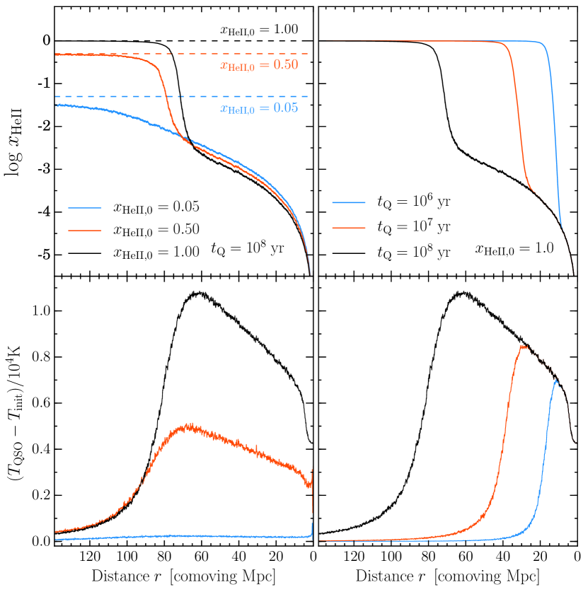
Figure 2.— Thermal evolution of the intergalactic medium around the quasar in different radiative transfer simulations. The upper panels show the evolution of the median fraction of singly ionized helium $x_{\rm HeII}$, while the bottom panels illustrate the evolution of the median temperature boost in the IGM. Left side panels show thermal evolution of the IGM as a function of initial He II fraction at a fixed quasar lifetime $t_{\rm Q}=10^{8}$ yr. Whilst right side panels show thermal evolution of the IGM as a function of different values of quasar lifetime while keeping fixed initial He II fraction $x_{\rm HeII,0}=1.0$. The dashed lines in the upper left panel indicate the values of initial He II fraction $x_{\rm HeII,0}$ in three different models. All median profiles are computed from $1000$ simulated skewers.

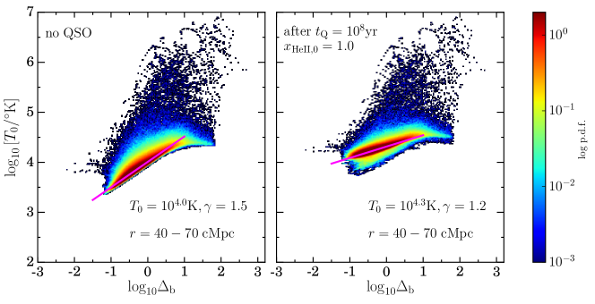
Figure 3.— Temperature-density relation in simulations. Left: prior to quasar turning on, right: in radiative transfer simulations after quasar has been on for $t_{\rm Q}=10^{8}$ yr in IGM with initial He II fraction $x_{\rm HeII,0}=1.00$. The relation is calculated at radial distances $r=40-70$ cMpc where the temperature boost is maximal in the models we consider (see Figure 2).

First, in Khrykin et al. (2016) we showed that the size of the He II proximity zone, where the He II fraction is greatly reduced by the quasar ionization front sweeping across the IGM, depends strongly on the quasar lifetime $t_{\rm Q}$. This is clearly shown in the upper right panel of Figure 2. The same lifetime dependence is manifest in the temperature profiles in the bottom right panel of Figure 2. This is because for longer lifetimes (e.g., $t_{\rm Q}=10^{8}$ yr) the quasar ionization front travels much further into the IGM, boosting the IGM temperature by $\Delta T\simeq 10^{4}$ K (in case of $x_{\rm HeII,0}=1.0$). In contrast, the quasar ionization front has not yet reached the same distance in the short lifetime model (e.g., $t_{\rm Q}=10^{6}$ yr), for which the size of the region is $\approx 4$ times smaller. In other words, the longer the IGM has been exposed to the quasar radiation, the larger the radial extent of the thermal proximity effect.

The panels at left in Figure 2 indicate that the IGM temperature in the quasar proximity zone also depends significantly on the amount of initially singly ionized helium, $x_{\rm HeII,0}$. It is apparent that if $x_{\rm HeII,0}=1.0$ (black curve), more hard photons emitted by the quasar photoheat the IGM and the median temperature is boosted by $\Delta T\simeq 10^{4}$ K, whereas there is no significant change in temperature if helium was already highly doubly ionized ($x_{\rm HeII,0}=0.05$) before the quasar turned on (blue curve). According to eqn. (13) $\Delta T\sim{\rm constant}\times\Delta x_{\rm HeII}\langle E\rangle$, hence, if $x_{\rm HeII}\simeq 0.05$, then the temperature boost will be much smaller. To summarize, whereas the quasar lifetime determines the size of the thermal proximity zone, the value of initial He II fraction sets the amplitude of the temperature boost in the zone.

Finally, it is apparent from bottom panels of Figure 2 that for fixed values of initial He II fraction and quasar lifetime the boost of IGM temperature is higher at larger distances from the quasar. This is due to the filtering of the intrinsic quasar spectrum by the IGM, which hardens the ionizing radiation field (Abel & Haehnelt, 1999; McQuinn et al., 2009; Bolton et al., 2009; Meiksin et al., 2010). Eqn. (13) indicates that the amount of heat input over the time-step $t$ is proportional to the average excess energy $\langle E\rangle$. Since the mean free path of He II ionizing photons scales as $\lambda_{\rm mfp}\propto\nu^{3}$, photons with energy near the edge $E_{\rm ion}\simeq h\nu\simeq 4$ Ry have a short mean free path. They, therefore, are preferably absorbed by the IGM very near the quasar resulting in a small value of $\langle E\rangle$. On the other hand, the high-energy photons can travel much further into the IGM before getting absorbed, owing to their sufficiently longer mean free path. They, thus inject more heat at larger distances from the quasar.

3.2. Temperature-Density Relation

Eqn. (8) indicates that the temperature of the intergalactic gas is determined by the competition between heating and cooling processes, dominated by the photoheating due to metagalactic UV background radiation and adiabatic cooling due to the expansion of the Universe. This competition results in a tight relation between the temperature and density of the (unshocked) gas which can be approximated by a power-law $T=T_{0}\Delta_{\rm b}^{\gamma-1}$ (for $\Delta_{\rm b}\leq 10$), where $T_{0}$ is the temperature at mean density, $\gamma$ is the power-law index, and $\Delta_{\rm b}=\rho/\bar{\rho}$ is the overdensity. This power-law index asymptotes to a value $\gamma\approx 1.6$ (Miralda-Escudé & Rees, 1994; Hui & Gnedin, 1997; Hui & Haiman, 2003; McQuinn et al., 2009; McQuinn & Upton Sanderbeck, 2016) several hundred Myr after reionization events.

It is expected that He II reionization will significantly change the temperature-density relation, tending to make it more isothermal, with $\gamma\longrightarrow 1$ (McQuinn et al., 2009; Compostella et al., 2013; La Plante et al., 2016). This is illustrated in Figure 3 where we compare the temperature-density relation from $1000$ skewers before quasar turns on (left panel) with their values after these skewers have been post-processed with our radiative transfer code, for a model with $t_{\rm Q}=10^{8}$ yr and $x_{\rm HeII,0}=1.00$ (right panel). The figure shows the temperature-density relation at distances $r=40-70$ cMpc from the quasar, where according to Figure 2 the temperature boost is maximal for the models we consider. Whereas the original hydrodynamical simulation resulted in temperature-density relation of ($T_{0}=10^{4}\,{\rm K}$, $\gamma=1.5$), the roughly density independent boost of $\Delta T\simeq 0.3$ dex in the proximity zone results in ($T_{0}=10^{4.3}\,{\rm K}$, $\gamma=1.2$). Similar effects are seen in full $3$D radiative transfer simulations of He II reionization (McQuinn et al., 2009; Compostella et al., 2013; La Plante et al., 2016).

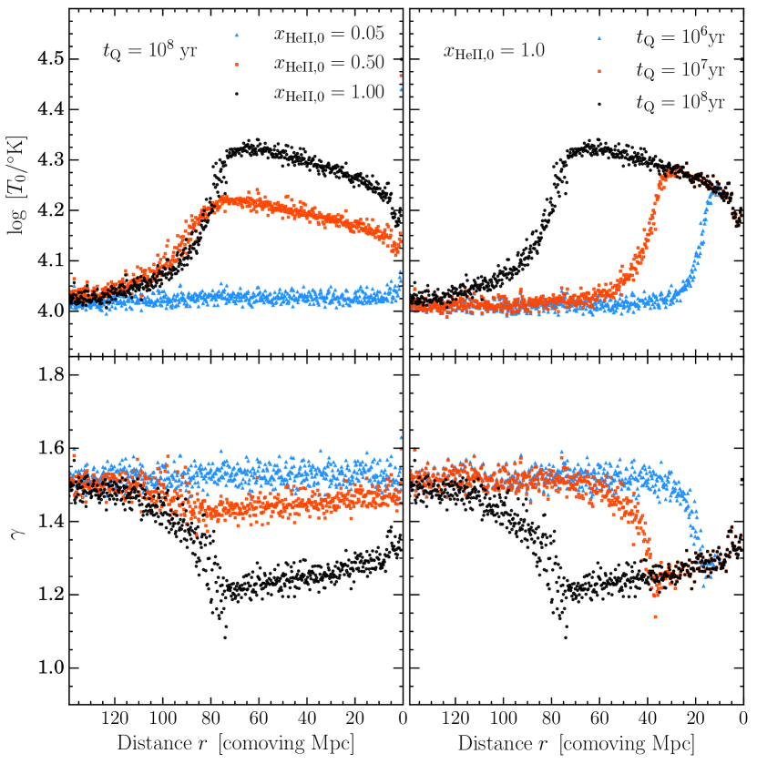
Figure 4.— Parameters of the temperature-density relation: temperature at mean density $T_{0}$ and the power-law index $\gamma$, for the same set of radiative transfer simulations as in Figure 2.

In order to study how the quasar radiation impacts the temperature-density relation with respect to our parameters of interest $t_{\rm Q}$ and $x_{\rm HeII,0}$ we fit the distribution of densities and temperatures in each pixel along $1000$ sightlines of models shown in Figure 2 with a power-law to calculate $T_{0}$ and $\gamma$. To reduce the scatter due to density fluctuations, we calculate the mean $T_{0}$ and $\gamma$ in bins of $20$ pixels, which corresponds to $\Delta r\simeq 0.25$ cMpc. The results are shown in Figure 4. As expected, the radial profile of $T_{0}$ and $\gamma$ closely follows that of the IGM temperature boost, which in turn reflects the dependencies on He II fraction and quasar lifetime described previously (see Figure 2).

The main effect of quasar radiation on the temperature-density relation is twofold. First, the intergalactic medium becomes much hotter due to additional heat injected by the quasar ionization front traversing through the IGM. This is reflected by the increase in $T_{0}$ by $\Delta T_{0}\simeq 0.3-0.4$ for $x_{\rm HeII,0}=1.00$ model and smaller temperature boosts for smaller He II fractions. Second, the temperature-density relation flattens in the quasar proximity zone with $\gamma$ deviating from the asymptotic value $\gamma=1.5$ (which prevailed in the IGM prior to quasar turning on; see left panel of Figure 3) towards the isothermal value of $\gamma=1$. As illustrated previously, the exact amplitude and extent of these changes strongly depend on the value of the initial He II fraction and quasar lifetime, as well as distance from the quasar in the thermal proximity zone. These trends are illustrated by the different curves in Figure 4.

To summarize, we investigated the dependence of the radial IGM temperature profile around quasars on the initial He II fraction $x_{\rm HeII,0}$ and the quasar lifetime $t_{\rm Q}$. We demonstrated that the radial extent of the elevated IGM temperatures probes the quasar lifetime, whereas the amplitude of the temperature boost is set by the amount of singly ionized helium in the IGM prior to the quasar turning on. Therefore the thermal proximity effect can be used to constrain both of these parameters and ultimately determine how quasar lifetime evolves with redshift, and the redshift at which He II reionization occurred. In what follows we describe a method to detect the thermal proximity effect and constrain these parameters.

4. Line-of-sight power spectrum statistics

Among the many methods used to study thermal evolution of the IGM the Ly$\alpha$ forest flux power spectrum is the most sensitive probe of the temperature of the gas in the IGM. This is due to the fact that thermal Doppler broadening affects the properties of the H I Ly$\alpha$ forest resulting in a prominent small-scale (high-$k$) cut-off in the power (McDonald et al., 2000; Zaldarriaga et al., 2001; Croft et al., 2002; Viel et al., 2009). In this section we show that by measuring the power spectrum in bins of radial distance from the quasar, one can detect the thermal proximity effect and constrain the He II fraction $x_{\rm HeII,0}$ and quasar lifetime $t_{\rm Q}$. In § 7 we also discuss another method to detect the thermal proximity effect based on wavelet analysis.

Recall Figure 2 where we showed that the amplitude and the extent of the thermal proximity effect around the quasar have a strong radial dependence which is sensitive to the quasar lifetime, and a temperature boost sensitive to the initial singly ionized fraction. Hence, the thermal broadening of the H I Ly$\alpha$ forest will be a function of quasar lifetime $t_{\rm Q}$, initial He II fraction $x_{\rm HeII,0}$ and distance $r$ from the quasar. Our approach is therefore to calculate the average H I Ly$\alpha$ forest power spectrum of a sample of quasars (we use a total number of $N=1000$ simulated H I Ly$\alpha$ spectra) in bins of $\Delta r=10$ cMpc and to compare the results with the power spectra from control regions far away from quasars and hence outside of their proximity zones. Very close to the quasar strong absorbers intrinsic to the quasar environment and shock-heated gas will complicate our analysis, and this galaxy formation physics will not be properly captured by our hydrodynamical simulations, hence we will exclude the first $3$ cMpc closest to the quasar along each line-of-sight.

The flux contrast along the line-of-sight can be written as

$$\delta F\left(x\right)=\frac{F\left(x\right)}{\langle F\rangle}-1,$$ (15)

where $F\left(x\right)={\rm exp}\left(-\tau\right)$ is the transmitted flux in each pixel $x$ of the skewer with optical depth $\tau$, and $\langle F\rangle$ is the mean flux of the IGM at any given redshift, for which we adopt measurements of Becker et al. (2013a). The line-of-sight power spectrum of the Ly$\alpha$ forest $P\left(k|r\right)$ as a function of wavenumber $k$ and distance from the quasar $r$ is then given by

$$P\left(k|r\right)=\langle\small|\delta\tilde{F}\left(k\right)\small|^{2}\rangle_{N}$$ (16)

where $\delta\tilde{F}\left(k\right)$ corresponds to the Fourier transform of $\delta F$ at wavenumber $k$, for a chunk of spectra in a $\Delta r=10$ cMpc at distance $r$ from the quasar, and angular brackets denote the averaging over total ensemble of skewers $N$. We adopt the common convention of working with the dimensionless power spectrum $\pi^{-1}kP\left(k|r\right)$. Note, given the described binning in radial direction, we cannot measure $k$-modes larger than the fundamental mode of the $10$ cMpc radial bin, hence the range of $k$-modes we consider is $k=\left[0.007,0.3\right]\ {\rm km^{-1}s}$, where $k_{\rm min}=2\pi/10\ {\rm cMpc}\simeq 0.007\ {\rm km^{-1}s}$ and $k_{\rm max}$ is limited to $k_{\rm max}\simeq 0.3\ {\rm km^{-1}s}$. The range of $k$ modes between $k_{\rm min}$ and $k_{\rm max}$ is also divided into $10$ bins that are equally spaced in ${\rm log}\ k$ space.

In the following sections we investigate the sensitivity of this power spectrum computed in radial bins to the value of the quasar lifetime, and the initial fraction of singly ionized helium.

4.1. Sensitivity to Quasar Lifetime

We compute three different models with $t_{\rm Q}=10^{6}$ yr, $t_{\rm Q}=10^{7}$ yr, and $t_{\rm Q}=10^{8}$ yr, while the value of the initial He II fraction is fixed to $x_{\rm HeII,0}=1.0$. The left columns of Figure 5 show simulated individual H I Ly$\alpha$ transmission spectra and temperature profiles in the proximity zone for these three models, calculated in three different radial bins, while the right column illustrates the corresponding H I Ly$\alpha$ power spectra averaged over $1000$ skewers in the same radial bins. The errorbars $\sigma_{\rm data}$, computed from $500$ random realizations of data power spectrum ($N=50$ skewers) drawn from original $1000$ skewers of the model with $t_{\rm Q}=10^{8}$ yr and $x_{\rm HeII,0}=1.00$, serve as an example of the constraining power of a realistic dataset . The bottom subpanels in the right column also show the difference $\Delta P$ in each radial bin between the power spectrum of each model and the power spectrum of our fiducial model (i.e., $t_{\rm Q}=10^{8}$ yr and $x_{\rm HeII,0}=1.00$) divided by the simulated error $\sigma_{\rm data}$. There are several trends that are immediately apparent from Figure 5.

First, in the bin closest to the quasar ($r=3-13$ cMpc) the time required by the ionization front to reach this distance and photoionize the gas is less than the quasar lifetimes for all three of the models shown. Thus, very close to the quasar the amplitude of the temperature boost is the same independent of the quasar lifetime (see Figure 2), and the resulting H I Ly$\alpha$ forest for these three lifetimes are indistinguishable in this bin, and the average power spectra are identical.

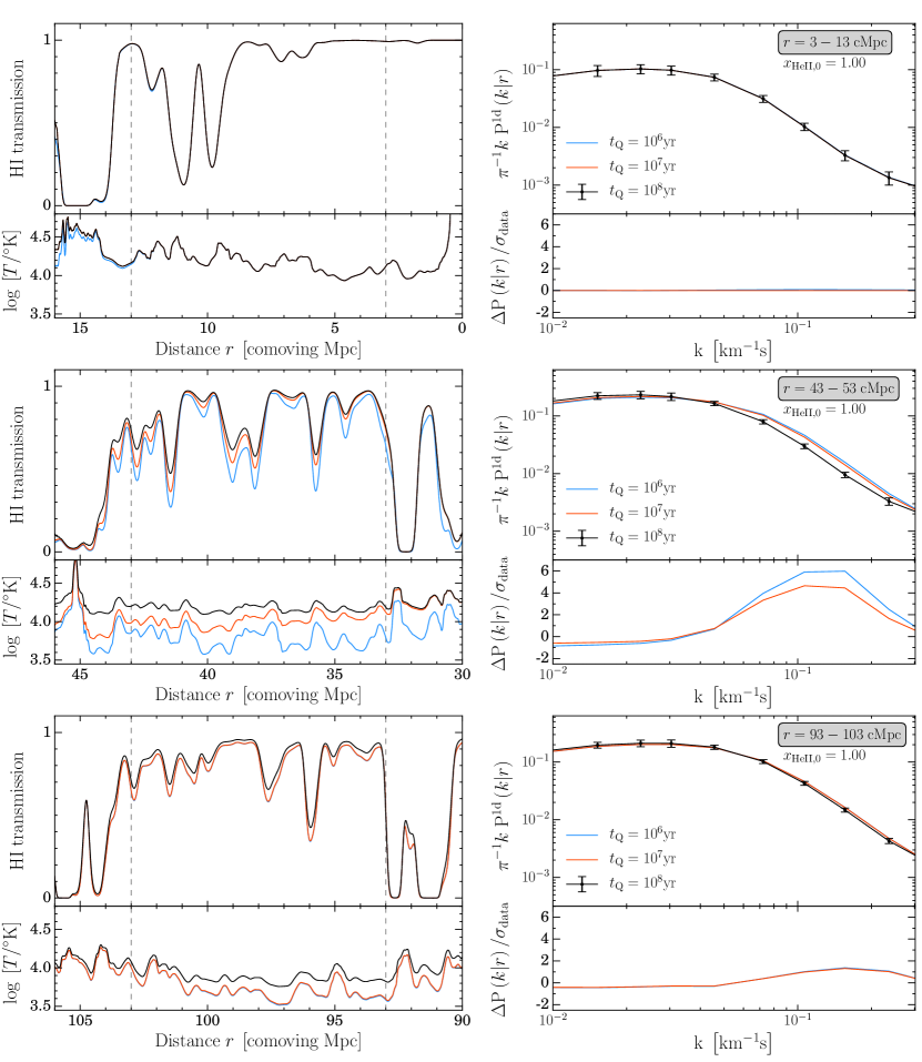
Figure 5.— Sensitivity of the H I Ly$\alpha$ forest power spectrum statistics to the value of quasar lifetime. Each row corresponds to the different radial bin from the quasar. Left column illustrates the simulated individual H I Ly$\alpha$ spectra (top) and IGM temperature profiles (bottom) for three models with $t_{\rm Q}=10^{6}$ yr (blue), $t_{\rm Q}=10^{7}$ yr (red) and $t_{\rm Q}=10^{8}$ yr (black). The value of initial fraction of singly ionized helium is fixed to $x_{\rm HeII,0}=1.0$ in all models. Right column shows the average H I Ly$\alpha$ power spectra (top subpanels) of the same models. The difference between the power spectrum of $t_{\rm Q}=10^{8}$ yr model and the other models divided by the simulated error (see text for explanation) is shown in the bottom subpanels.

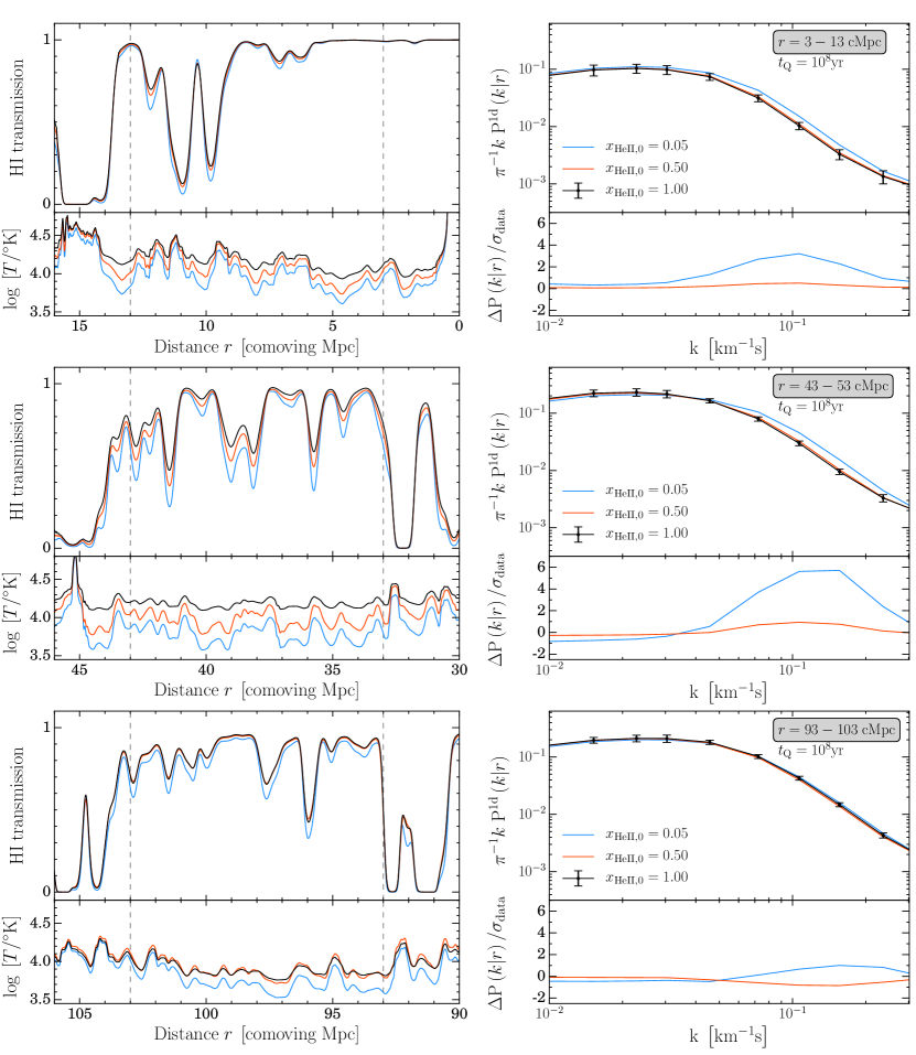
Figure 6.— Sensitivity of the H I Ly$\alpha$ forest power spectrum statistics to the value of initial He II fraction. Three models are plotted with initial He II fraction $x_{\rm HeII,0}=0.05$ (blue), $x_{\rm HeII,0}=0.50$, and $x_{\rm HeII,0}=1.00$. The lifetime of quasar is fixed in all models to $t_{\rm Q}=10^{8}$ yr. See Figure 5 for the description of the panels.

However, further away from the quasar the difference between power spectra increases. It is apparent that at an intermediate distance $r=43-53$ cMpc the Ly$\alpha$ forest spectra and temperature profiles of the three models differ significantly. For the longest lifetime model the quasar ionization front has already traversed and ionized gas at this distance and boosted the IGM temperature by $\Delta T\approx 10^{4}$ K (see Figure 2), whereas it has not yet reached this distance in models with shorter quasar lifetime ($t_{\rm Q}=10^{7}$ yr and $t_{\rm Q}=10^{6}$ yr). Thus, the temperature of this region of the IGM is lower in these models, than in $t_{\rm Q}=10^{8}$ yr model. This difference in the IGM temperature produces different amounts of thermal broadening in the Ly$\alpha$ forest, that is why the H I Ly$\alpha$ forest of the longest lifetime model becomes smoother and contains less saturated absorption features, than H I Ly$\alpha$ spectra of cooler models. Accordingly, the power spectrum of the $t_{\rm Q}=10^{8}$ yr models exhibits less small-scale power (high-$k$), because it is smoothed out by the thermal broadening. Thus, we conclude that there is considerably more small-scale power ($k\gtrsim 0.05\ {\rm km^{-1}s}$) in models with shorter quasar lifetimes. The differences between the power spectra in this radial bin, illustrated in the bottom subpanel, shows that these models should be easily distinguishable.

Finally, far away from the quasar at $r\simeq 93-103$ cMpc the difference between the power spectra of $t_{\rm Q}=10^{6}$ yr and $t_{\rm Q}=10^{7}$ yr models diminishes again because there was not enough time for the quasar ionization front to reach and ionize gas at this distance, and significantly change the temperature of the IGM, whereas the thermal proximity zone for the $t_{\rm Q}=10^{8}$ yr model extends out to $r\sim 100$ cMpc and still exhibits a small boost $\Delta T\approx 10^{3}$ K (see Figure 2). Hence the $t_{\rm Q}=10^{6}$ yr and $t_{\rm Q}=10^{7}$ yr models are indistinguishable in this bin and the gas is at the ambient IGM temperature, whereas these models differ from the $t_{\rm Q}=10^{8}$ yr model.

4.2. Sensitivity to initial He II Fraction

Similarly, we now investigate the sensitivity of the line-of-sight Ly$\alpha$ power spectrum statistics to the variations of the initial He II fraction. Akin to the discussion in previous section we run three radiative transfer simulations, each with different values of the initial He II fraction $x_{\rm HeII,0}=0.05$, $x_{\rm HeII,0}=0.50$, and $x_{\rm HeII,0}=1.00$, respectively. The quasar lifetime is fixed to $t_{\rm Q}=10^{8}$ yr. Figure 6 illustrates the resulting H I Ly$\alpha$ transmission, IGM temperature profiles and power spectra of these models in the same radial bins as Figure 5.

In § 2.3 we showed that the initial He II fraction determines the amplitude of the temperature boost in the proximity zone (see left panels of Figure 2). Thus, one naturally expects to see significant differences in the properties of the H I Ly$\alpha$ forest and its power spectrum between models with very different values of $x_{\rm HeII,0}$. Indeed, one can see from the left column of Figure 6 that the temperature of the IGM significantly differs between the considered models (reaching maximum $\Delta T\approx 10^{4}$ K at $r\simeq 43-53$ cMpc). As expected, the temperature boost in the proximity zone is maximized in the $x_{\rm HeII,0}=1.00$ model (black). On the contrary, as explained in Section 2.3, the temperature of the IGM hardly changes if helium is predominantly highly doubly ionized before the quasar turns on ($x_{\rm HeII,0}=0.05$, blue curve). Analogous to the discussion in Section 4.1, this difference in the photoheating results in different amount of thermal broadening of the H I Ly$\alpha$ forest, therefore affecting the power spectra of the models, i.e. decreasing the small-scale power in the hotter model ($x_{\rm HeII,0}=1.00$) in comparison to the cooler one ($x_{\rm HeII,0}=0.05$).

Interestingly, the difference between the power spectra of the $x_{\rm HeII,0}=1.00$ (black) and two models with $x_{\rm HeII,0}=0.05$ (blue) and $x_{\rm HeII,0}=0.50$ (red) first increases as one goes from the bin closest to the quasar ($r=3-13$ cMpc) to the intermediate bin ($r=43-53$ cMpc) and decreases afterward as one goes to the outskirts of the proximity zone ($r=93-103$ cMpc). This behavior is driven by two effects. First, as we noted in Section 3, the intergalactic medium filters quasar radiation, which results in more heat injected at larger distances from the quasar, than close to it (see Figure 2). Consequently, the thermal broadening of the H I Ly$\alpha$ forest lines is strongest at the intermediate distance $r=43-53$ cMpc ($\Delta T\approx 10^{4}$ K). Hence, the difference between the average power spectra illustrated in the right columns of Figure 6 follows similar behavior. However, recall that the radial extent of the boost of the IGM temperature depends on the value of quasar lifetime, which is fixed to $t_{\rm Q}=10^{8}$ yr in all models considered here. As we showed in Section 4.1 the temperature of the IGM is increased only at distances $r$ for which the quasar ionization front has had enough time to travel to and ionize the gas. At further distances from the quasar, the temperature asymptotes to the level of the ambient IGM (see right panels in Figure 2). Therefore, at the largest radii the power spectra of all three models approach each other and the differences are significantly smaller.

We have demonstrated the sensitivity of the H I Ly$\alpha$ forest power spectrum to the parameters defining the radial extent and the amplitude of the thermal proximity effect: quasar lifetime $t_{\rm Q}$ and the initial fraction of singly ionized helium $x_{\rm HeII,0}$. We now proceed to estimate the accuracy with which we can constrain these parameters by applying a Bayesian MCMC analysis to a mock sample of H I Ly$\alpha$ forest power spectra.

5. Estimation of the quasar lifetime and He II fraction

Our subsequent analysis of the H I Ly$\alpha$ forest power spectrum assumes that the temperature of the ambient IGM in regions far away from active quasars has already been measured to high precision. Hence, in what follows we imagine that the hydrodynamical simulations that we use as the input to our radiative transfer calculations are designed to reproduce these temperature measurements, and thus to have the correct temperature-density relation in the IGM prior to when the quasars responsible for the thermal proximity effect turned on. Although the ambient IGM’s temperature-density relation may very well be determined by similar thermal proximity effects from a previous generation of quasars, we can nevertheless imagine that the quasars whose proximity zones we study at any epoch turned on in an IGM whose thermal state is precisely known. Assuming that the outputs from our hydrodynamical simulations have been calibrated in this way, we then perform radiative transfer calculations for different combinations of $t_{\rm Q}$ and $x_{\rm HeII,0}$. Given the dependence of the H I Ly$\alpha$ forest power spectrum on these parameters (see Section 4), we compare the power spectra of different models and therefore deduce the precision with which quasar lifetime and initial He II fraction can be determined. We make no attempt to model or marginalize out uncertainties on the thermal state of the ambient IGM. In what follows we describe the basic aspects of our method and begin with the definition of the likelihood required by the MCMC algorithm.

5.1. The Likelihood

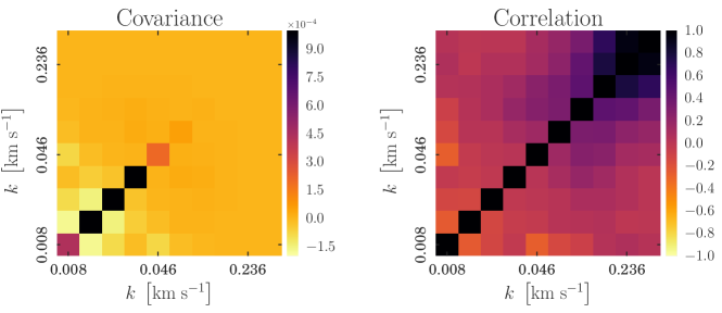
Figure 7.— Example of the covariance and correlation matrices in a single radial bin $r=63-73$ cMpc (see eqn. 18-19) for the data sample is drawn from the model with $t_{\rm Q}=10^{8}$ yr and $x_{\rm HeII,0}=1.0$.

We construct a grid of $81$ models at $z=3.9$ ($1000$ skewers per model) with combination of initial He II fraction and logarithmically spaced quasar lifetime values, where $x_{\rm HeII,0}=\left[0.05,0.10,0.20,0.30,0.50,0.60,0.70,0.90,1.00\right]$ and ${\rm log}\left(t_{\rm Q}/{\rm Myr}\right)=\left[0.0,0.25,0.5,0.75,1.0,1.25,1.5,1.75,2.0\right]$. Further, similar to the discussion in § 4, we choose the data sample to be represented by $N=50$ H I Ly$\alpha$ spectra. In what follows we perform MCMC inference for $9$ different data samples, each represented by $50$ H I Ly$\alpha$ spectra drawn from one model with one combination of $\{x_{\rm HeII,0}^{\rm data},{\rm log}\ t_{\rm Q}^{\rm data}\}$, where $x_{\rm HeII,0}^{\rm data}=\left[0.05,0.5,1.0\right]$ and ${\rm log}\left(t_{\rm Q}^{\rm data}/{\rm Myr}\right)=\left[0.0,1.0,2.0\right]$. It is well known that the distribution of power spectrum measurements is well described by a multi-variate Gaussian distribution, and following the standard approach (McDonald et al., 2006; Palanque-Delabrouille et al., 2013), we adopt the following form for our likelihood of the data power spectrum given the model in each radial bin:

$$\mathscr{L}^{\rm bin}\left\{P_{\rm data}\left(k|r\right)|x_{\rm HeII,0},{\rm log}\ t_{\rm Q},r\right\}=\left(2\pi\right)^{-{\rm N_{\rm k}}/2}\times$$

$${\rm det}\left(\Sigma\right)^{-1/2}{\rm exp}\Bigg{(}-\frac{1}{2}\bigg{[}P_{\rm data}\left(k|r\right)-P_{\rm model}\left(k|r\right) \bigg{]}^{\rm T}$$

$$\times\Sigma_{\rm bin}^{-1}\bigg{[}P_{\rm data}\left(k|r\right)-P_{\rm model}\left(k|r\right)\bigg{]}\Bigg{)},\$$ (17)

where $N_{\rm k}$ is the number of band powers that we consider in each radial bin, $P_{\rm data}\left(k|r\right)$ is the average power spectrum of $N=50$ data skewers in each radial bin, $P_{\rm model}\left(k|r\right)$ is the average power spectrum of each model on the grid in $2$D parameter space in this radial bin (calculated from $N=1000$ skewers), and $\Sigma_{\rm bin}$ is the covariance matrix of the data power spectrum in the corresponding radial bin. The covariance is given by

$$\Sigma_{\rm bin}\left(k,k^{\prime}\right)=\Bigg{\langle}\Big{[}P_{\rm data}\left(k|r\right)-\langle P\left(k|r\right)\rangle\Big{]}\times$$

$$\Big{[}P_{\rm data}\left(k^{\prime}|r\right)-\langle P\left(k^{\prime}|r\right)\rangle\Big{]}\Big{\rangle}_{\rm N}$$ (18)

where $\langle P\left(k|r\right)\rangle$ is the average power spectrum of $1000$ skewers drawn from the model with the same parameters as the data subsample. For each of the 9 different models (different combinations of $\{x_{\rm HeII,0},{\rm log}\ t_{\rm Q}\}$) for which we perform MCMC inference, the covariance matrix $\Sigma_{\rm bin}$ is computed by calculating $P_{\rm data}$ from $N=500$ random realizations of $N=50$ data skewers drawn from each model. An example of the covariance and correlation matrices given by eqn. (18) is shown in Figure 7 for a model with $t_{\rm Q}=10^{8}$ yr and $x_{\rm HeII,0}=1.00$, where the correlation matrix illustrates the degree of correlation between pairs of pixels $\{k,k^{\prime}\}$ and defined as

$$R_{\rm bin}\left(k,k^{\prime}\right)=\frac{\Sigma_{\rm bin}(k,k^{\prime})}{\sqrt{\Sigma_{\rm bin}(k,k)\Sigma_{\rm bin}(k,k^{\prime})}}$$ (19)

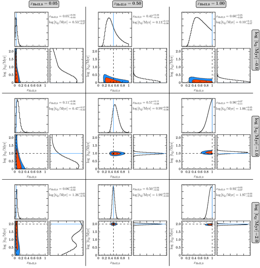
Figure 8.— Constraints on quasar lifetime and initial He II fraction from the MCMC analysis. The labels on top of each column and on the right side of each row show the values of initial He II fraction and quasar lifetime in the sample of $N=50$ skewers representing data. The $95\%$ (red) and $68\%$ (blue) confidence levels from MCMC calculations are shown in each panel. The dashed lines show the values of lifetime and He II fraction in the sample representing data. The quoted values of $x_{\rm HeII,0}$ and $t_{\rm Q}$ are the $16$th, $50$th and $84$th percentiles of the corresponding marginalized distributions.

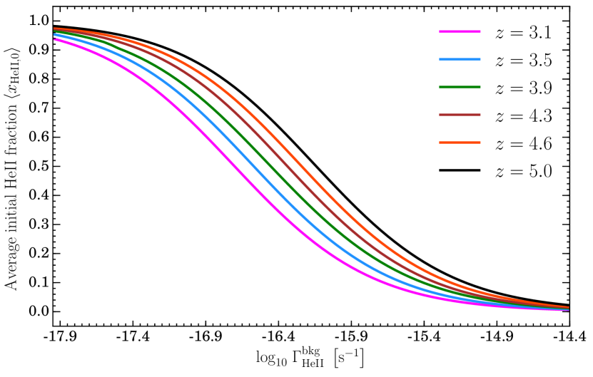
Figure 9.— Average initial He II fraction $\langle x_{\rm HeII,0}\rangle$ in our radiative transfer calculations as a function of the assumed He II ionizing background (see Section 2 for details) for each value of redshift we consider. The parameter grids at each redshift were constructed in accordance to this dependence.

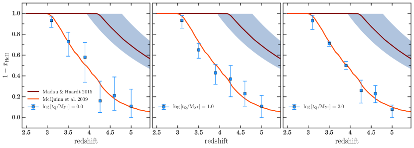
Figure 10.— Reconstructed history of He II reionization, quantified by the fraction of completely doubly ionized helium $x_{\rm HeIII}\equiv 1-x_{\rm HeII}$. Each panel corresponds to assumed value of quasar lifetime in the data samples, i.e., $t_{\rm Q}=10^{6}$ yr (left), $t_{\rm Q}=10^{7}$ yr (middle), and $t_{\rm Q}=10^{8}$ yr (right), respectively. The solid lines in all three panels illustrate the results of the simulations of He II reionization history: red - McQuinn et al. (2009), brown - Madau & Haardt (2015) ($1\sigma$ variance in their models is illustrated by grey shaded area). The blue data points in each panel show the results of our calculations, specifically the $50th$ percentile from MCMC $1$D posterior distributions of $x_{\rm HeII,0}^{\rm data}$. The errorbars indicate $16{\rm th}$ and $84{\rm th}$ percentiles of the same distributions (see Section 5.2 for details), respectively. The number of spectra used in data sample at redshifts $z=\left[3.1,3.5,3.9\right]$ is $N=50$, while at $z=\left[4.3,4.6,5.0\right]$ $N=20$, based on the number of available to date quasar spectra.

Following eqn. (17) we can compute the likelihood of the data power spectrum in each radial bin inside the thermal proximity region for any given model. The full likelihood of the data in the proximity zone is then calculated multiplying the corresponding likelihoods in each radial bin, yielding

$$\mathscr{L}^{\rm full}\left(P_{\rm data}\left(k|r\right)|x_{\rm HeII,0},{\rm log}\ t_{\rm Q}\right)=\prod_{i=1}^{\rm M}\mathscr{L}^{\rm bin}_{i}$$ (20)

where ${\rm M}=11$ is the number of $10\ {\rm cMpc}\ r$-bins used (from $r=3$ cMpc to $r=113$ cMpc). Eqn. (20) is valid under the assumption that the correlations between the power spectra in the neighboring radial bins are small or negligible. We justify this assumption in Appendix A, to which we refer the interested reader. We use eqn. (20) to calculate $\mathscr{L}^{\rm full}$ at each point in our parameter grid, and then use bivariate spline interpolation to estimate $\mathscr{L}^{\rm full}$ for any combination of $\{{\rm log}\ t_{\rm Q},\ x_{\rm HeII,0}\}$ between the grid points in this $2$D parameter space.

5.2. MCMC

Having arrived at an expression for the likelihood of each model given by eqn. (17) and eqn. (20), and being able to evaluate the likelihood in any location of the $\{{\rm log}\ t_{\rm Q},\ x_{\rm HeII,0}\}$ $2$D parameter space, we can now explore this likelihood with MCMC to determine the posterior distributions of our parameters. This, in turns, allows us to estimate the accuracy with which we can measure the mean quasar lifetime $t_{\rm Q}$ and initial He II fraction $x_{\rm HeII,0}$ from the sample of $N=50$ data spectra. For these purposes we apply publicly available affine invariant MCMC ensemble sampling algorithm emcee presented and described in Foreman-Mackey et al. (2013).

Following the algorithm described in § 5.1 we perform MCMC parameter inference on the $N=50$ data spectra drawn from each of 9 different models. The results of this inference are illustrated in Figure 8, where each panel shows results for each of the 9 models. The columns in Figure 8 show different initial He II fractions $x_{\rm HeII,0}^{\rm data}=\left[0.05,0.50,1.00\right]$, whereas the rows are for different values of quasar lifetime ${\rm log}\left(t_{\rm Q}^{\rm data}/{\rm Myr}\right)=\left[0.0,1.0,2.0\right]$. The contours illustrate the $95\%$ (blue) and $68\%$ (red) confidence levels, respectively. Marginalized parameter distributions for $t_{\rm Q}$ and $x_{\rm HeII,0}$ are also shown by the histograms. We compute the $16$th, $50$th and $84$th percentiles of these marginalized distributions, which are quoted as the measurement ($50$th percentile), and the lower and upper error bars ($16$th and $84$th percentile) in each panel. There are several notable trends.

First, consider the case where the IGMs initial He II fraction is low ($x_{\rm HeII,0}^{\rm data}=0.05$; left column). According to Figure 2 there is no significant heating of the gas due to the quasar turning on, independent of the quasar lifetime value. Consequently, the power spectrum of these models are not significantly different and the left column of Figure 8 illustrates that the quasar lifetime is essentially unconstrained. Nevertheless, the lack of a significant thermal proximity effect constrains the initial He II fraction to be small, with the typical absolute errors on $x_{\rm HeII}$ around $\delta_{x_{\rm HeII,0}}\simeq 0.04$.

Previously we argued that temperature boost is stronger in models with longer quasar lifetimes and higher values of initial He II fraction (see Figure 2). Hence, the thermal broadening of the H I Ly$\alpha$ forest follows the same dependence on $t_{\rm Q}$ and $x_{\rm HeII,0}$, as reflected by the power spectra in Figures 5-6. As a result, our MCMC parameter constrains on $t_{\rm Q}^{\rm data}$ and $x_{\rm HeII,0}^{\rm data}$ improve when the thermal proximity effect in the H I Ly$\alpha$ forest is both larger in size (longer $t_{\rm Q}$), and when the temperature boost is larger (larger $x_{\rm HeII,0}$). This is illustrated by the middle and right columns of Figure 8, where we show results of MCMC calculations for two different values of initial He II fraction, i.e., $x_{\rm HeII,0}^{\rm data}=0.50$ (middle column) and $x_{\rm HeII,0}^{\rm data}=1.00$ (right-hand column). For instance, because the radial size of the thermal proximity region is small if the quasar lifetime is only $t_{\rm Q}=10^{6}$ yr, the absolute error of the MCMC constraints on the He II fraction is $\delta_{x_{\rm HeII,0}}\approx 0.20$ (for $x_{\rm HeII,0}^{\rm data}=0.50$ and $x_{\rm HeII,0}^{\rm data}=1.00$). However, as the quasar lifetime becomes longer (i.e, $t_{\rm Q}^{\rm data}=10^{7}$ yr and $t_{\rm Q}^{\rm data}=10^{8}$ yr) the size of the thermal proximity zone becomes larger, and, hence, the thermal proximity effect is more prominent. Hence, the mean absolute errors of the MCMC constraints on $x_{\rm HeII}$ shrink down to $\delta_{x_{\rm HeII,0}}\approx 0.10$ if the quasar lifetime is $t_{\rm Q}=10^{7}$ yr, and to $\delta_{x_{\rm HeII,0}}\approx 0.05$ in case of $t_{\rm Q}=10^{8}$ yr, respectively. Similar trends are apparent for the constraints on quasar lifetime, for which the mean absolute error is $\delta_{{\rm log}t_{\rm Q}}\approx 0.1$ dex when $t_{\rm Q}^{\rm data}\gtrsim 10^{7}$ yr and $x_{\rm HeII,0}^{\rm data}=1.00$.

Finally, in Khrykin et al. (2016) we illustrated the degeneracy, which exists between $t_{\rm Q}$ and the He II ionizing background $\Gamma_{\rm HeII}^{\rm bkg}$. This degeneracy significantly complicates any constraints on $t_{\rm Q}$ or $x_{\rm HeII,0}$ one can obtain from the direct measurements of the He II proximity zones sizes in far ultraviolet quasar spectra. We argued that this degeneracy can be broken if the value of $\Gamma_{\rm HeII}^{\rm bkg}$ can be determined from the measurements of He II effective optical depth. However, these measurements become impossible at $z\gtrsim 4$ making it challenging to determine $t_{\rm Q}$ and $x_{\rm HeII,0}$ from direct observations of He II proximity zones. On the other hand, as illustrated in Section 3, these parameters should not be strongly degenerate for the thermal proximity effect, because $t_{\rm Q}$ determines the radial size of the thermal proximity zone and $x_{\rm HeII,0}$ sets the amplitude of the temperature boost. Figure 8 illustrates that this is indeed the case because the contours in each panel of Figure 8 are aligned with the $x_{\rm HeII}$ and ${\rm log}\ t_{\rm Q}$ directions on the axes.

Given the high sensitivity of our method to the value of the IGM He II fraction, our study opens up the exciting possibility of determining the timing of He II reionization without direct UV observations of He II Ly$\alpha$ absorption at $z\gtrsim 4$, which are currently impossible. The obvious next question is how well can we reconstruct the full He II reionization history with the thermal proximity effect, which we address in the next section.

6. Reconstructing the He II Reionization History

We apply our thermal proximity effect power spectrum method and perform MCMC inference on mock datasets extracted from the same set of hydrodynamical + radiative transfer simulations at $z=\left[3.1,3.5,3.9,4.3,4.6,5.0\right]$ ($1000$ skewers per redshift). Similar to Section 5.1, we construct the same grid of models for each redshift, covering values of initial He II fraction $x_{\rm HeII,0}=\left[0.05-1.00\right]$ and logarithmically spaced quasar lifetimes ${\rm log}\left(t_{\rm Q}/{\rm Myr}\right)=\left[0.00-2.00\right]$. Figure 9 illustrates the dependence of the average initial He II fraction at different redshifts on the value of the He II ionizing background, which sets the initial He II fraction $x_{\rm HeII,0}$ prior to when the quasar turns on. The value of H I ionizing background $\Gamma_{\rm HI}^{\rm bkg}$ is adjusted at each redshift in order to match the mean transmission in the H I Ly$\alpha$ forest measured by Becker et al. (2013a). Following the discussion in Section 5.1, we compute the power spectra of all models averaged over $1000$ skewers at each redshift.

After the grid of average power spectra is computed at all redshifts, the remaining missing ingredient, necessary for the likelihood calculations and MCMC analysis (see Section 5), is the sample of modeled spectra representing the data at each redshift $z$. For this we adopt the values of $x_{\rm HeII,0}^{\rm data}$ from the fiducial model of He II reionization from McQuinn et al. (2009) (see model D1 in the bottom panel of their Figure 3), resulting in the following values of He II fraction in the data samples at each redshift

$$z=3.1:\ \ x_{\rm HeII,0}^{\rm data}=0.03;\ z=4.3:\ \ x_{\rm HeII,0}^{\rm data}=0.70$$

$$z=3.5:\ \ x_{\rm HeII,0}^{\rm data}=0.30;\ z=4.6:\ \ x_{\rm HeII,0}^{\rm data}=0.80$$

$$z=3.9:\ \ x_{\rm HeII,0}^{\rm data}=0.50;\ z=5.0:\ \ x_{\rm HeII,0}^{\rm data}=0.90$$

We consider three values of quasar lifetime in the data samples, i.e., ${\rm log}\left(t_{\rm Q}^{\rm data}/{\rm Myr}\right)=\left[0.0,1.0,2.0\right]$. Finally, we note that the number of existing archival high-resolution spectra at $z\simeq\left[4.3,4.6,5.0\right]$ is less than the fiducial number $N=50$ that we used in our analysis in previous sections. A more realistic choice is $N=20$ at these higher redshifts, which we adopt for the data samples at these redshifts, whereas for $z=\left[3.1,3.5,3.9\right]$ we use the same fiducial number of spectra $N=50$ as before.

Using eqn. (17)-(20) we perform MCMC parameter inference at each redshift, resulting in marginalized posterior distributions for $x_{\rm HeII,0}$. Analogous to Section 5.2, we compute the $16$th, $50$th and $84$th percentiles of these distributions, and use those to define the measured value of $x_{\rm HeII,0}^{\rm data}$ ($50$th percentile) and its uncertainties ($16$th and $84$th percentiles). Figure 10 illustrates our reconstructions of the He II reionization history, shown by the fraction of completely ionized helium $x_{\rm HeIII}\equiv 1-x_{\rm HeII}$. The three panels correspond to the different values of the quasar lifetime that were assumed for the data, i.e., ${\rm log}\left(t_{\rm Q}^{\rm data}/{\rm Myr}\right)=0.0$ (left), ${\rm log}\left(t_{\rm Q}^{\rm data}/{\rm Myr}\right)=1.0$ (middle), and ${\rm log}\left(t_{\rm Q}^{\rm data}/{\rm Myr}\right)=2.0$ (right), respectively. The red solid curves in each panel show McQuinn et al. (2009) He II reionization history (red), whereas the brown solid curve (and grey uncertainty region) are the default and modified He II reionization histories for the semi-analytical reionization model of Madau & Haardt (2015), in which the active galactic nuclei dominate the reionization process resulting in an early He II reionization by the same population of sources that reionized intergalactic hydrogen. The blue dots with error bars are the results of our calculations. It is apparent from Figure 10 that exploiting the thermal proximity effect in H I Ly$\alpha$ forest around quasars can be used to fully reconstruct the He II reionization history, and constrain both its timing and duration.

7. Thermal Proximity Effect: Wavelet Analysis

Another approach to quantifying the thermal proximity effect is to use wavelets. Wavelets are filters that are local in both Fourier and configuration space, allowing one to select the modes of interest as a function of distance from the quasars. There is a rich history of applying wavelets to the Ly$\alpha$ forest to measure the mean temperature as well as to search for temperature fluctuations (Theuns & Zaroubi, 2000; Zaldarriaga, 2002; Lidz et al., 2010). We can use our previous power spectrum calculations to design a wavelet to select modes that contain much of the discriminating information that the power spectrum analysis is using. Based on a qualitative analysis of Figures 5-6, we chose our wavelet to be a Gaussian filter centered at $k_{0}=0.13\ {\rm km^{-1}s}$ with a standard deviation of $\sigma_{k}=0.04\ {\rm km^{-1}s}$, roughly the wavenumbers where the power spectra of the different models for the thermal proximity effect differ the most. Note that an offset Gaussian kernel in Fourier space is a phase times a Gaussian in configuration space:

$$W_{M}(x)=\exp\left[ik_{0}x\right]\times\exp\left[-\frac{x^{2}\sigma_{k}^{2}}{2}\right].$$ (21)

This form for the wavelet filter, termed the Morlet wavelet, is convolved with our different models for the flux. We consider the “wavelet power” as a function of distance:

$$a(r)^{2}=\left[\int W\left(r-r^{\prime}\right)F\left(r^{\prime}\right)dr^{\prime}\right]^{2}.$$ (22)

We then smooth $a\left(r\right)^{2}$ with a Gaussian kernel with standard deviation $200\,{\rm km\ s^{-1}}$ ($\approx 2.5$ cMpc at $z=3.9$) to generate a smoothed field, $\langle a\left(r\right)^{2}\rangle_{200}$ that is plotted in Figure 11. Note that our normalization of $\langle a\left(r\right)^{2}\rangle_{200}$ has no physical significance.

Before we discuss the results, we comment on the advantages and disadvantages of the wavelet approach relative to the power spectrum analysis used in the rest of the paper. A clear advantage is that the locality of this filter in configuration space (having width $\sim 1/\sigma_{k}$ which for our choice is $25\ {\rm km\ s^{-1}}$) has the nice property that the data do not have to be binned into distance intervals. This allows one to detect trends with distance from the quasar, even in the absence of a model. This feature could be particularly useful well into He II reionization, when the heating profile around quasars is likely to be more complicated than we have assumed (McQuinn et al., 2009). Disadvantages include that (1) it is somewhat more difficult to estimate posteriors as adjacent wavelet coefficients are correlated, (2) our wavelet, in contrast to the power spectrum, does not use all discriminating information in 2-point correlations, and (3), in our experience, it is easier to diagnose systematics in the power spectrum (as it is easier to diagnose systematics when focusing on a range of wavenumbers).

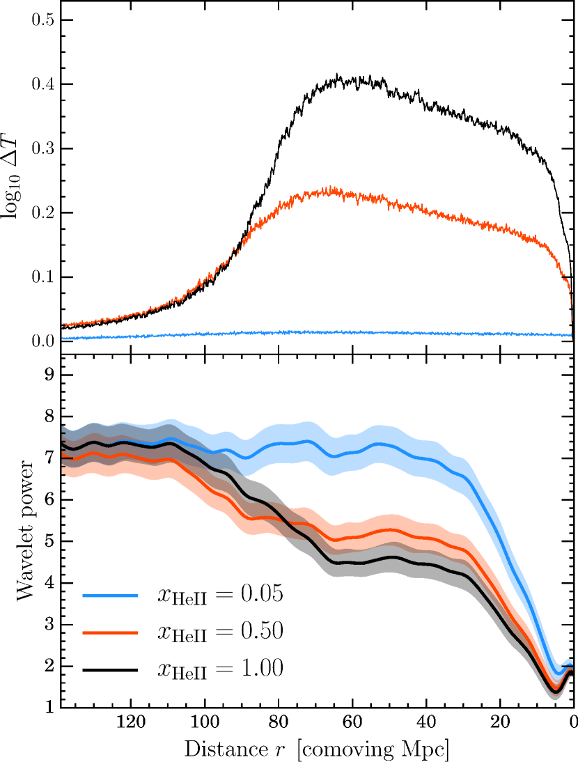
Figure 11.— Upper panel: Median temperature profiles for three models with $t_{\rm Q}=10^{8}$ yr, but different initial He II fraction: $x_{\rm HeII,0}=0.05$ (blue), $x_{\rm HeII,0}=0.50$ (red), $x_{\rm HeII,0}=1.00$ (black), similar to Figure 2. Bottom panel: wavelet coefficients for the same models using $N=1000$ simulated H I Ly$\alpha$ spectra. The shaded areas are the $1\sigma$ error bars calculated from $500$ random realizations of $N=50$ skewers representing the data samples drawn from each of the models.

With these words of caution, we proceed to apply the wavelet to our models with quasar lifetime fixed at $t_{\rm Q}=10^{8}$ yr and different initial He II fractions of $x_{\rm HeII,0}=\left[0.05,0.50,1.00\right]$ (the same models as in Figure 5). The median of the temperature in these models is shown in the top panel of Figure 11. The average wavelet coefficient as a function of distance from the quasar at $z=3.9$ are shown in the bottom panel of Figure 11, with each curve calculated from $N=1000$ mock H I spectra. The shaded regions are the $1\sigma$ range from $50$ quasars, calculated using $500$ random realizations. It is apparent, that at large distances all models asymptote to the same power. However, at smaller distances, i.e. $r\lesssim 90\ {\rm cMpc}$ – the radial extent of the thermal proximity region –, the three models show different wavelet power levels at a level that should be distinguishable with $50$ spectra, and the $x_{\rm HeII,0}=0.05$ model can be distinguished from the others with far fewer spectra. Furthermore, the radial trends in the wavelet power trace the temperature and extent of the models’ thermal proximity effect. At smaller radii still, $r\lesssim 20\ {\rm cMpc}$, the effect of the quasar being in an overdense location is apparent in all three cases as a suppression in the wavelength power.

In conclusion, a wavelet thermal proximity effect analysis is able to distinguish between the models that we consider with a similar number of quasar spectra as that required for a power spectrum analysis. Since trends in the wavelet coefficient are more easily understood than trends in the power spectrum, any claimed detection of a thermal proximity effect in the power spectrum should be reinforced with a wavelet analysis. Wavelets further enable a more model-independent search for thermal proximity regions than the analysis advocated in previous sections.

8. Discussion

In this section we discuss systematics relevant for detecting the thermal proximity effect and placing robust constraints on He II fraction and quasar lifetime. In addition, we discuss several assumptions that went into our previous estimates and how they affect our conclusions.

8.1. The Uniformity of the He II Ionizing Background

Throughout this work we have assumed that the He II ionizing background is constant in space and time, and added it in each pixel along simulated skewers. Here we note that, except for possibly when $x_{\rm HeII}\ll 1$, a pervasive and uniform background flux is likely not a good approximation. Our methodology of including a uniform background photoionization rate is a convenience to maintain the desired $x_{\rm HeII}$ at the mean density. Since the He III $\rightarrow$ He II recombination time is comparable to the age of the Universe, the effect of this background on our results is minimal and our results would not change if we turned it off (as motivated in § 2, we also do not include the photoheating from this background). We also note that when $x_{\rm HeII}$ is appreciably different from unity, we expect each quasar to be turning on in a swiss cheese of relic He III regions. The approximation of a uniform $x_{\rm HeII}$ is meant to describe the average effect. Since our analysis ultimately stacks measurements from many quasars and since we are concerned with reionization and heating – which are linear in $\Delta x_{\rm HeII}$ (see eqn. 13) – we expect the thermal proximity profile in a stack of real sightlines to be reasonably approximated by the stack of quasars going off in a medium with uniform ionizing background and $x_{\rm HeII}$.

8.2. Initial Thermal State of the IGM

As discussed at the beginning of § 5.1, our calculations assume perfect knowledge of the thermal state of the IGM before the quasar turns on, and that the hydrodynamical simulations we compare to have been calibrated to reproduce this thermal state of the ambient IGM using data far from quasars. However, note that the thermal state of the ambient IGM is set by the He II reionization history. For example, a quasar turning on in an IGM which has an average $x_{\rm HeII,0}=0.05$ implies that He II was already reionized by an earlier generation of quasars (or other sources). In this case, the IGM around the quasar should have already been photoheated to higher temperature by the earlier reionization of He II. Therefore for a model with $x_{\rm HeII,0}=0.05$, quasars would turn on in an IGM which is actually initially hotter than a $x_{\rm HeII,0}=1.00$ model, for which there was not yet any He II reionization heating. This $x_{\rm HeII,0}$ dependent initial thermal state has not been modeled in our calculations.

The sensitivity of the power spectrum analysis presented here depends on the amount of heat $\Delta T$ that was injected into the IGM by quasar radiation (see discussion in § 4) relative to the initial temperature of the IGM. Therefore, our analysis is likely sensitive to the initial IGM thermal state. If the temperature of the ambient IGM is much higher (lower) than what we have assumed in our models, the precision of our MCMC constraints in § 5.2 could be over-estimated (under-estimated). Throughout this work we used the outputs of hydrodynamical simulations with the value of ambient IGM temperature $T_{0}\simeq 10^{4}$ K, which is probably too low in case when initial He II fraction is $x_{\rm HeII,0}=0.05$ as outlined previously.

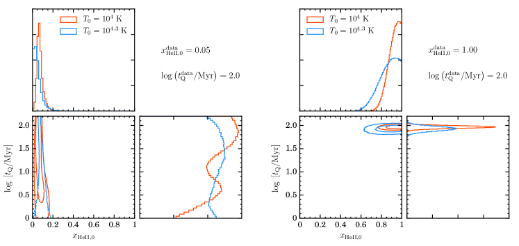
Figure 12.— Constraints on $x_{\rm HeII,0}$ and $t_{\rm Q}$ from the MCMC analysis in case of increased initial IGM temperature for $x_{\rm HeII,0}^{\rm data}=0.05$ (left) and $x_{\rm HeII,0}^{\rm data}=1.00$ (right). The bottom left subpanels illustrate the $95\%$ and $68\%$ confidence intervals on $x_{\rm HeII,0}$ and $t_{\rm Q}$ for two cases: (1) analogous to Figure 8 when $T_{0}\simeq 10^{4}$ K (red), and (2) increased initial IGM temperature $T_{0}\simeq 10^{4.3}$ K (blue). The top and bottom right subpanels show the marginalized parameter distributions.

For this reason and in order to verify the sensitivity of our analysis to the level of initial IGM temperature, we increase $T$ in all pixels along $1000$ skewers drawn from hydrodynamical simulations at $z=3.9$ by $\Delta T=7000^{\circ}$K, and then run our radiative transfer calculations and construct the same grid of models as in § 5.1. Adding this $\Delta T$ mimics the heating produced by He II reionization, naturally flattening the temperature-density relation as expected due to the roughly density independent injection of heat (see § 3.2). It also leaves temperatures effectively unchanged in hot shock-heated regions. Similar to the discussion in § 5.1, we estimate the likelihood of two data samples of $N=50$ skewers drawn from the models with the same value of quasar lifetime $t_{\rm Q}^{\rm data}=10^{8}$ yr, but different initial He II fractions, i.e., $x_{\rm HeII,0}^{\rm data}=0.05$ and $x_{\rm HeII,0}^{\rm data}=1.0$. We explore these likelihoods with our MCMC analysis (see 5.2).

The results of this test are shown in Figure 12, where we compare the results of MCMC analysis in case of increased initial temperature of the IGM to those we obtained previously in § 5.2. The left side panels show the results in case $x_{\rm HeII,0}^{\rm data}=0.05$, whereas the right side panels are for $x_{\rm HeII,0}^{\rm data}=1.0$. It is apparent from Figure 12 that, similar to the bottom left panel in Figure 8, when $x_{\rm HeII,0}^{\rm data}=0.05$ there is no sensitivity to quasar lifetime due to lack of thermal proximity effect, but the constraints we obtain on initial He II fraction given increased initial temperature of the IGM ($x_{\rm HeII,0}=0.04^{+0.04}_{-0.02}$) are comparable to those in § 5.2. On the other hand, Figure 12 illustrates that in case $x_{\rm HeII,0}^{\rm data}=1.0$ the constraining power of our analysis is decreased by $\simeq 50\%$ when compared to results in § 5.2. This is due to the fact that the heat injection $\Delta T$ (see eqn. 13) is smaller, hence the thermal proximity effect in the H I Ly$\alpha$ forest is weaker. However, keep in mind that we have actually modeled a rather extremely high temperature for $x_{\rm HeII,0}^{\rm data}=1.00$ case (as our initial temperature of $T_{0}\simeq 10^{4.3}$ K is motivated by expectations for when most of the He II had been reionized).

Lastly, our analysis largely ignores the complicated radiative transfer and heating that is expected during the last half of He II reionization as the ionizing regions largely overlap and hard photons heat locations far from quasars (McQuinn et al., 2009; Compostella et al., 2013). The trends with radius should be weaker than at the earlier times studied here, when proximate heating dominates the radial trend. Modeling the morphology of this heating likely requires full $3$D calculations, and non-parametric wavelet methods are likely more suited to this more model dependent case.

8.3. Continuum Placement and the Mean Flux

Another systematic that could affect the thermal proximity effect inferences is the placement of the quasar continuum. Throughout this work we have assumed perfect knowledge of the quasar continuum, but misplacement of the quasar continuum could lead to systematic errors in the power spectrum measurements which are at the heart of our method to measure the thermal proximity effect. Although continuum fitting uncertainties are relatively small ($\sim$ few per cent) at $z\simeq 2-3$ using high-resolution data, they can reach $\simeq 10-20\%$ at $z\gtrsim 4$ (Faucher-Giguère et al., 2008). Furthermore, the thermal proximity effect falls on the tail of the quasar’s broad Ly$\alpha$ line, thus the continuum errors could be significantly larger at this location in the spectrum.

To explore how the continuum placement affects power spectrum estimates, let us define a different flux contrast field $\delta F_{\rm C}$ as follows

$$\delta F_{\rm C}\left(r\right)=\frac{F(r)-\langle F\rangle_{\rm local}}{\langle F\rangle_{\rm local}}=\frac{f_{\rm obs}(r)/C-\langle f_{\rm obs}/C\rangle_{\rm local}}{\langle f_{\rm obs}/C\rangle_{\rm local}}$$ (23)

where $C$ is the continuum flux, $F$ is the transmitted flux, and $\langle F\rangle_{\rm local}=\langle f_{\rm obs}/C\rangle_{\rm local}$ is the mean flux in the $10$ cMpc radial bin under consideration. Note that $\langle F\rangle_{\rm local}$ is estimated not from an ensemble of quasars, but rather from each individual quasar spectrum. Whereas our original definition of flux contrast $\delta F$ (eqn. 15) implicitly assumed perfect knowledge of the continuum and the mean flux, this new $\delta F_{\rm C}$ suffers from additional noise, because $\langle F\rangle_{\rm local}$ is a noisy estimate of the true mean flux $\langle F\rangle$ due to fluctuations on $\sim 10$ cMpc scales. This method of local continuum fitting is analogous to the “trend-removal” approach adopted in previous Ly$\alpha$ forest studies (Hui et al., 2001; Croft et al., 2002; Lidz et al., 2006, 2010). However, if the continuum $C$ is roughly constant over this $10$ cMpc $r$-bin, then according to the definition of $\delta F_{\rm C}$ in eqn. (23), $C$ cancels out and the power spectrum is insensitive to the continuum level. Even if $C$ is not exactly constant, it is very likely that the continuum does not contribute much power on scales smaller than $10$ cMpc, and so our new $\delta F_{\rm C}$ will be insensitive to continuum errors. We now redo our analysis to see if the reduced information in $\delta F_{\rm C}$ (eqn. 23) relative to $\delta F$ (eqn. 15) affects our results.

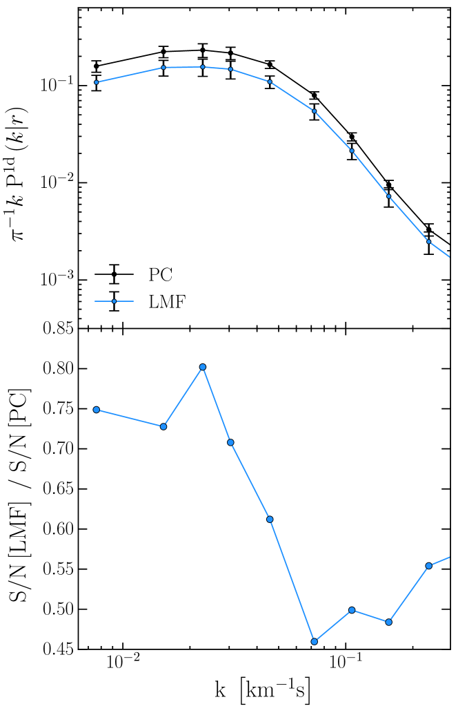
Figure 13.— Comparison between the power spectra of the H I Ly$\alpha$ forest at $r=43-53$ cMpc from the quasar, calculated in two methods. In the upper panel the solid black line shows the case when the perfect knowledge of the quasar continuum (“PC”) is assumed (similar to black curve in the middle panel of Figure 5), while the blue curve illustrates the results of the local mean flux (“LMF”) analysis (see discussion in the text for details). In both cases the power spectra are computed from $1000$ skewers drawn from the model with $t_{\rm Q}=10^{8}$ yr and $x_{\rm HeII,0}=1.00$. The errorbars are computed from 500 random realizations of data power spectrum drawn from original 1000 skewers of the each model. The bottom panel shows the ratio of signal-to-noise ratios in two cases.

Using the new flux contrast $\delta F_{\rm C}$, we perform our calculations from § 5 for the case of $N=50$ skewers, with $t_{\rm Q}^{\rm data}=10^{8}$ yr, and $x_{\rm HeII,0}^{\rm data}=1.0$. We compute the average power spectrum $P_{\rm data}\left(k|r\right)\equiv\langle|\delta\tilde{F}_{\rm C}(k)|^{2}\rangle$. We then calculate the likelihood of this data sample in each radial bin we consider, and perform parameter inference with MCMC. The results of this modified analysis, to which we refer as “LMF” (Local Mean Flux), are shown in Figure 13, where we present power spectra of the H I Ly$\alpha$ forest in the $r=43-53$ cMpc radial bin of the thermal proximity region (see middle panel of Figures 5-6).

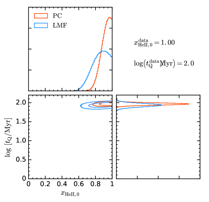
Figure 14.— Comparison between the constraints on $x_{\rm HeII,0}$ and $t_{\rm Q}$ obtained from the MCMC analysis in two methods. The bottom left panel shows the $95\%$ and $68\%$ confidence intervals on $x_{\rm HeII,0}$ and $t_{\rm Q}$ in case when (1) similar to Figure 8, the perfect knowledge of the quasar continuum is assumed (“PC”), which is shown in red, and (2) when the local mean flux (“LMF”) is used in models instead, which is shown in blue. The top and bottom right panels show the marginalized parameter distributions for $x_{\rm HeII,0}$ and ${\rm log}\ t_{\rm Q}$, respectively. The solid red histograms are for the PC case, while the solid blue ones illustrate the LMF approximation.

The black curve in the upper panel of Figure 13 shows the power spectrum of the $t_{\rm Q}=10^{8}$ yr, $x_{\rm HeII,0}=1.0$ model (averaging $1000$ skewers), calculated assuming perfect knowledge of the quasar continuum (the same as in § 4, which we refer to as “PC” - Perfect Continuum). The blue curve shows the power spectrum of the same model calculated using the LMF (eqn. 23). The errorbars are computed from $500$ random realizations of data power spectrum drawn from original $1000$ skewers of each model. The bottom panel shows the ratio of the signal-to-noise ratio (S/N) for the two methods defined as $\Delta=[P_{\rm model}/\sigma]_{\rm LMF}/[P_{\rm model}/\sigma]_{\rm PC}$. The power spectrum and the error bars on the data power spectrum are reduced when we calculate the mean flux locally. This is apparent from the bottom panel of Figure 13, where one can see that at $k\gtrsim 2\times 10^{-2}\ {\rm km^{-1}s}$ the ${\rm S/N}$ ratio has dropped by $\approx 50\%$ for the LMF case relative to the previous results of § 4.

Figure 14 shows the results of MCMC calculations for the same data sample for two methods, i.e., the red contours illustrate the results for the global mean flux used in the power spectrum calculations, whereas the blue contours are for the LMF case. It is apparent that our analysis of the thermal proximity effect has lost about half of its constraining power, but nevertheless still allows robust constraints on both quasar lifetime $t_{\rm Q}$ and initial He II fraction $x_{\rm HeII,0}$. The reason why the constraints have weakened by this amount is that the LMF method has made us insensitive to the thermal proximity effect’s impact on the average transmission profile (remember $x_{\rm HI}\propto T^{-0.7}$ and so the mean absorption in the forest is modulated by the thermal proximity effect), and because $\delta F_{\rm C}$ suffers from additional noise due to fluctuations of $\langle F\rangle_{\rm local}$ about the true mean flux.

To conclude, we have presented two distinct cases. First, we assumed perfect knowledge of the quasar continuum, which gives the best possible constraints. Second, we analyzed the worst case scenario when there is no knowledge of the quasar continuum in the thermal proximity region. In this case, despite the drop in overall constraining power of our method, we were still able to constrain the parameters of interest. Note however that in principle, one could jointly model both the power spectrum and the mean flux profile in the thermal proximity zone, effectively mitigating the extra noise present in the LMF case.

8.4. Degeneracy with Photon Production Rate $Q_{\rm 4Ry}$

In § 3.1 we have illustrated how the radial size of the thermal proximity region depends on the quasar lifetime $t_{\rm Q}$. In practice, the size of this region is correlated with the distance $r_{\rm IF}$ to which the quasar ionization front traveled in time $t=t_{\rm Q}$. Given that the recombination time is long compared to the quasar lifetimes we consider in this work ($t_{\rm Q}\ll t_{\rm rec}\simeq 10^{9}$ yr), the location of the quasar ionization front is approximately proportional to the product of quasar lifetime and quasar photon production rate, i.e., $r_{\rm IF}\propto\left(t_{\rm Q}\times Q_{\rm 4Ry}\right)^{1/3}$. Hence, in practice, the radial size of the thermal proximity region must depend on a degenerate combination of $t_{\rm Q}$ and $Q_{\rm 4Ry}$, or the total number of ionizing photons emitted.

However, in this work we have ignored this degeneracy by fixing $Q_{\rm 4Ry}$ to a single value and illustrated the effect of quasar lifetime only. While this might seem to be an unnecessary simplification, we note that, in reality, the degeneracy between $t_{\rm Q}$ and $Q_{\rm 4Ry}$ can be broken. This is because the average quasar SED directly constraints the quasar apparent magnitude $m_{912}$ at the Lyman limit $\lambda=912{\rm\AA}$, which, given the knowledge of the quasar SED slope $\alpha_{\rm 1Ry\rightarrow 4Ry}$ between $1$ Ry and $4$ Ry (Telfer et al., 2002; Shull et al., 2012; Lusso et al., 2015), can be used to estimate the quasar photon production rate at $4$ Ry $Q_{\rm 4Ry}$. The most uncertain thing is the slope of quasar SED above $4$ Ry $\alpha_{\rm 4Ry\rightarrow\infty}$, which can change $Q_{\rm 4Ry}$ by $\approx 25-45\%$ (Khrykin et al., 2016). However, the $z\simeq 3$ He II Ly$\alpha$ proximity effect can be used to calibrate $\alpha_{\rm 4Ry\rightarrow\infty}$ using stacked proximity zone profiles (Khrykin et al., 2016). Note also that although quasars have different luminosities, we are sensitive to the average quantities only in our analysis of the thermal proximity effect. Thus, we argue that constraints on the average quasar luminosity that can be calibrated with the observations, will allow one to determine the average quasar lifetime using the thermal proximity effect.

8.5. The Dependence on the Spectral Slope $\alpha_{\nu}$

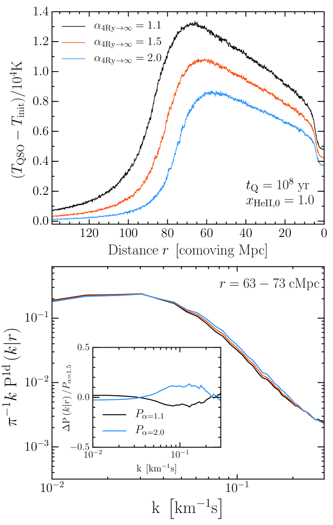
Figure 15.— Thermal evolution of the intergalactic medium around the quasar in different radiative transfer simulations. The upper panel shows the evolution of the median IGM temperature profiles (similar to the bottom panels of Figure 2) as a function of the slope of the quasar SED at $\nu\geq\nu_{\rm 4Ry}$ $\alpha_{\rm 4Ry\rightarrow\infty}$, whilst the bottom panel illustrates the resulting average power spectra of the same models in $r=63-73$ cMpc radial bin. The embedded panel shows the percent change in the power spectra compared to the power spectrum of our fiducial model with $\alpha_{\rm 4Ry\rightarrow\infty}=1.5$. Each curve is a stack of a $1000$ skewers. The quasar lifetime and the initial He II fraction in each model are $t_{\rm Q}=10^{8}$ yr and $x_{\rm HeII,0}=1.0$, respectively.

Throughout the paper we have assumed a constant slope of the quasar SED $\alpha_{\nu}$ at frequencies blueward of $1$ Ry, with $\alpha_{\nu}=1.5$. However, the spectral slope regulates the number of high-energy photons with long mean free path, therefore any change in $\alpha_{\nu}$ can affect the IGM temperature and H I transmission at large distances from the quasar (see discussion in § 3). As we discussed in § 8.4, the photon production rate $Q_{\rm 4Ry}$ can be constrained from observations given our good knowledge of the spectral slope between $1$ and $4$ Ry. However, the slope beyond $4$ Ry is currently not well defined. In order to investigate how variations in the slope of the quasar SED above $4$ Ry affect our results, we have run an additional set of radiative transfer simulations, and in what follows we describe our findings.

Analogous to the discussion in Khrykin et al. (2016), we fix the quasar specific photon production rate $N_{\rm 4Ry}$ (see eqn. 1), which is calculated from the observable specific photon production rate $N_{\rm 1Ry}$ at $1$ Ry extrapolated as a power law to $4$ Ry assuming a spectral slope $\alpha_{\rm 1Ry\rightarrow 4Ry}=1.5$, consistent with recent constraints from quasar SED (Telfer et al., 2002; Shull et al., 2012; Lusso et al., 2015). We then change the SED slope from $4$ Ry to infinity within the range $\alpha_{\rm 4Ry\rightarrow\infty}=1.1-2.0$, and run our radiative transfer algorithm.

The upper panel of Figure 15 illustrates the effect of varying the slope of quasar SED $\alpha_{\rm 4Ry\rightarrow\infty}$ on the median IGM temperature profiles. The quasar lifetime and initial He II fraction are set to $t_{\rm Q}=10^{8}$ yr and $x_{\rm HeII,0}=1.00$ in all models. As expected (see discussion in § 3), smaller (larger) values of $\alpha_{\rm 4Ry\rightarrow\infty}$ increase (decrease) the number of hard photons produced by the quasar, and hence change the amount of energy injected into the IGM, dramatically altering the amplitude of the thermal proximity effect. Namely, the maximum temperature boost is a factor of $2$ higher (lower) in case when $\alpha_{\rm 4Ry\rightarrow\infty}=1.1$ ($\alpha_{\rm 4Ry\rightarrow\infty}=2.0$), compared to the fiducial model with $\alpha_{\rm 4Ry\rightarrow\infty}=1.5$. It is also apparent that the peak of the temperature profile shifts toward larger distances from the quasar when the spectral slope becomes harder (i.e., $\alpha_{\rm 4Ry\rightarrow\infty}=1.1$). Since the mean free path of ionizing photons scales as $\lambda_{\rm mfp}\propto\nu^{3}$, the high-energy photons can travel further into the IGM, depositing their energy at larger distances, and because there are more such photons for a harder SED shape ($\alpha_{\rm 4Ry\rightarrow\infty}=1.1$), the peak shifts.

On the other hand, the bottom panel of Figure 15 illustrates the resulting average line-of-sight H I power spectra for the same models. It is apparent that the variations in $\alpha_{\rm 4Ry\rightarrow\infty}$ result in only modest differences in the power spectrum ($\Delta P/P_{\alpha=1.5}\simeq 10\%$). These are substantially smaller than the uncertainties in the continuum placement discussed in § 8.3. Hence, we argue that variations in $\alpha_{\rm 4Ry\rightarrow\infty}$ should not affect our analysis of the thermal proximity effect significantly.

Finally, we remind the reader that the slope of quasar SED above $4$ Ry can be calibrated with the lower-$z$ He II Ly$\alpha$ proximity zone profiles (Khrykin et al., 2016). Alternatively, it is also possible to constrain the spectral index $\alpha_{\rm 4Ry\rightarrow\infty}$ by modeling the He II ionizing background at $2.5\leq z\leq 3.5$ and comparing it to $\Gamma_{\rm HeII}^{\rm bkg}$ estimated from measurements of He II effective optical depth at the same redshifts (Khaire, 2017).

9. Conclusions

We combined cosmological hydrodynamical simulations with $1$D radiative transfer calculations to investigate the line-of-sight thermal proximity effect and its detectability in H I Ly$\alpha$ forest absorption spectra. The hard radiation emitted by quasars photoionizes He II in their environment, and the resulting photoelectric heating boosts the temperature of the surrounding IGM. We showed how the radial temperature profile around quasars depends on the quasar lifetime, $t_{\rm Q}$, and the average He II fraction, $x_{\rm HeII,0}$, in the IGM before the quasar turned on. The main conclusions of our work are:

1. The amplitude of the thermal proximity effect depends strongly on the average amount of singly ionized helium, which prevailed in the IGM prior to the quasar activity, $x_{\rm HeII,0}$, whereas the size of the thermal proximity zone depends on the average quasar lifetime, $t_{\rm Q}$.

2. We presented a new method to detect this temperature boost, and thus constrain $x_{\rm HeII,0}$ and $t_{\rm Q}$, by measuring the H I power spectrum of an ensemble of quasar spectra as a function of distance from the quasar (in several $\sim 10$ cMpc bins), and comparing the results to control regions far away from the quasar. We also discussed another method based on the wavelet analysis, which enables a non-parametric study of the thermal proximity effect.

3. Combining our power spectrum method with a Bayesian MCMC formalism, we showed that a mock dataset of $50$ quasars at $z\sim 4$ can be used to measure the mean quasar lifetime $t_{\rm Q}$ to a precision of $\sim 0.1$ dex, and the initial fraction of singly ionized helium $x_{\rm HeII,0}$ to an (absolute) precision of up to $\sim 0.05$.

4. Our calculations show that existing H I Ly$\alpha$ forest datasets can use line-of-sight thermal proximity effect to reconstruct the full He II reionization history over the redshift range $3.1\leq z\leq 5.0$, constraining the timing and duration of He II reionization.

5. We discussed several sources of uncertainties that affect the constraining power of our analysis, including the initial thermal state of the IGM and uncertainties in the continuum spectra of quasars. We found that even under the most extreme assumptions, the constraining power of our method decreases by at most a factor of $\approx 2$.

Reconstruction of the He II reionization history over $3\lesssim z\lesssim 5$ with our method would in turn provide a global census of hard ($>4$ Rydberg) ionizing photons in the high-$z$ Universe. Besides being fundamental for understanding He II reionization, this census would have important implications for the thermal state of the IGM, the luminosity density of quasars and AGN (or other sources of hard photons), possibly even H I reionization (Madau & Haardt, 2015; D’Aloisio et al., 2016).

10. Acknowledgements

We would like to thank members of the ENIGMA group at the Max-Planck-Institut für Astronomie (MPIA) for useful discussions and comments on the paper. We are grateful to the anonymous referee for comments and suggestions, which greatly improved the text. I.S.K. thanks Martin Haehnelt for useful discussion about the mean flux issues and Michael Walther for his assistance. I.S.K. acknowledges support from the grant of the Ministry of Education and Science of the Russian Federation №$3.858.2017$. M.M. acknowledges support from NSF through grant AST 1514734 and NASA through grant HSTAR-13903.00.

Appendix A Appendix A: Cross-Correlations and the Inference Test

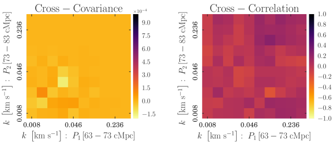
Figure 16.— Cross-covariance (left panel) and cross-correlation (right panel) matrices for two neighboring bins: $r_{1}=63-73$ cMpc and $r_{2}=73-83$ cMpc. The data sample is drawn from the model with $t_{\rm Q}=10^{8}$ yr and $x_{\rm HeII,0}=1.0$.

In order to estimate the full likelihood of a given data sample in the thermal proximity region (see Section 5.1), we assumed that the cross-correlation terms in the multivariate Gaussian distribution, describing the correlations between the power spectra in neighboring radial bins, are small and can safely be neglected. Thus, according to eqn. (20), the full likelihood is just the product of likelihoods in each radial bin inside the thermal proximity region.

In order to validate the above assumption we calculate the cross-correlation of the power spectrum between the neighboring radial bins and check if the cross-correlations are indeed small. For this consider two $10\ {\rm cMpc}\ r$-bins, i.e., $r_{1}$ and $r_{2}$, in which we calculate data power spectra $P_{1}\left(k\right)$ and $P_{2}\left(k^{\prime}\right)$, respectively (each is the average of the same $N=50$ skewers). The cross-correlation $\rho\left[P_{1}\left(k\right),P_{2}\left(k^{\prime}\right)\right]$ between power spectra in these two radial bins is then given by

$$\rho\left[P_{1}\left(k\right),P_{2}\left(k^{\prime}\right)\right]=\frac{\Sigma\left[P_{1}\left(k\right),P_{2}\left(k^{\prime}\right)\right]}{\sigma_{P_{1}\left(k\right)}\times\sigma_{P_{2}\left(k^{\prime}\right)}}$$ (A1)

where $\Sigma\left[P_{1}\left(k\right),P_{2}\left(k^{\prime}\right)\right]$ is the cross-covariance matrix

$$\begin{split}\Sigma\left[P_{1}\left(k\right),P_{2}\left(k^{\prime}\right)\right]=\Big{\langle}\left[P_{1}\left(k|r\right)-\langle P_{1}\left(k|r\right)\rangle\right]\times\\ \times\left[P_{2}\left(k^{\prime}|r\right)-\langle P_{2}\left(k^{\prime}|r\right)\rangle\right]\Big{\rangle}_{\rm N}\end{split}$$ (A2)

estimated from $N=500$ random samples of $P_{1}\left(k\right)$ and $P_{2}\left(k^{\prime}\right)$ with replacements, $\sigma_{P_{1}\left(k\right)}$ and $\sigma_{P_{2}\left(k^{\prime}\right)}$ are the diagonal elements of the respective auto-covariance matrix (in the corresponding bins $r_{1}$ and $r_{2}$) for each of the power spectra $P_{1}\left(k\right)$ and $P_{2}\left(k^{\prime}\right)$, respectively.

Figure 16 shows an example of cross-covariance $\Sigma\left[P_{1}\left(k\right),P_{2}\left(k^{\prime}\right)\right]$ and cross-correlation $\rho\left[P_{1}\left(k\right),P_{2}\left(k^{\prime}\right)\right]$ matrices between data power spectra in two radial bins: $r_{1}=63-73$ cMpc and $r_{2}=73-83$ cMpc. It is apparent from Figure 16 that cross-correlations between the power spectra in neighboring bins are small, i.e., $\lesssim\pm 15-20\%$, but not exactly negligible. We note that the same behavior holds for any combination of neighboring radial bins. Therefore, in order to check the robustness of the results obtained in Section 5.2 for the covariance matrix (see eqn. 18) which does not include these cross-correlations we perform a simple inference test, described in what follows.

We calculate the power spectrum of the data sample consisting, as previously, of a realization of $N=50$ skewers taken from the model at $z=3.9$ with ${\rm log}\ t_{\rm Q}^{\rm data}=1.50$ and $x_{\rm HeII,0}^{\rm data}=0.50$. Following the procedure described in Section 5.1, we calculate the full likelihood of this data sample using the covariance matrix given by eqn. (18), which ignores the cross-correlation terms. We then run the MCMC algorithm in order to obtain the posterior distributions of ${\rm log}\ t_{\rm Q}$ and $x_{\rm HeII,0}$. We repeat this inference procedure for $N_{\rm samples}=500$ different random realizations of the $N=50$ skewers in the data sample, and ask how often the true value of the parameters, i.e., ${\rm log}\ t_{\rm Q}^{\rm data}=1.50$ and $x_{\rm HeII,0}^{\rm data}=0.50$, falls inside the $68\%$ and $95\%$ contours of the MCMC posterior distributions. If our inference is indeed robust, the fraction of realizations lying inside these contours should correspond to the probability level of these contours in the posterior, i.e., $\sim 68\%$ and $\sim 95\%$, respectively. The inference test recovers the probability to encounter true values of ${\rm log}\ t_{\rm Q}$ and $x_{\rm HeII,0}$ inside the $\sim 68\%$ contour is $P\left(68\%\right)\simeq 66.4\%$ and for $\sim 95\%$ contour is $P\left(95\%\right)\simeq 92.8\%$, respectively. Thus, since these probabilities are so close to the ideal case, the assumption that we can neglect the cross-correlation terms holds, and demonstrates the robustness of our likelihood, MCMC, and inference procedure.

References

- Abel & Haehnelt (1999) Abel, T., & Haehnelt, M. G. 1999, ApJ, 520, L13
- Anderson et al. (1999) Anderson, S. F., Hogan, C. J., Williams, B. F., & Carswell, R. F. 1999, AJ, 117, 56
- Araya & Padilla (2014) Araya, I. J., & Padilla, N. D. 2014, MNRAS, 445, 850
- Bajtlik et al. (1988) Bajtlik, S., Duncan, R. C., & Ostriker, J. P. 1988, ApJ, 327, 570
- Becker et al. (2011) Becker, G. D., Bolton, J. S., Haehnelt, M. G., & Sargent, W. L. W. 2011, MNRAS, 410, 1096
- Becker et al. (2013a) Becker, G. D., Hewett, P. C., Worseck, G., & Prochaska, J. X. 2013a, MNRAS, 430, 2067
- Bolton et al. (2012) Bolton, J. S., Becker, G. D., Raskutti, S., et al. 2012, MNRAS, 419, 2880
- Bolton et al. (2010) Bolton, J. S., Becker, G. D., Wyithe, J. S. B., Haehnelt, M. G., & Sargent, W. L. W. 2010, MNRAS, 406, 612
- Bolton et al. (2009) Bolton, J. S., Oh, S. P., & Furlanetto, S. R. 2009, MNRAS, 395, 736
- Borisova et al. (2015) Borisova, E., Lilly, S. J., Cantalupo, S., et al. 2015, ArXiv e-prints, arXiv:1510.00029
- Compostella et al. (2013) Compostella, M., Cantalupo, S., & Porciani, C. 2013, MNRAS, 435, 3169
- Compostella et al. (2014) —. 2014, MNRAS, 445, 4186
- Croft et al. (2002) Croft, R. A. C., Weinberg, D. H., Bolte, M., et al. 2002, ApJ, 581, 20
- D’Aloisio et al. (2016) D’Aloisio, A., Upton Sanderbeck, P. R., McQuinn, M., Trac, H., & Shapiro, P. R. 2016, ArXiv e-prints, arXiv:1607.06467
- Davies et al. (2016) Davies, F. B., Furlanetto, S. R., & McQuinn, M. 2016, MNRAS, 457, 3006
- Fan et al. (2006) Fan, X., Strauss, M. A., Becker, R. H., et al. 2006, AJ, 132, 117
- Faucher-Giguère et al. (2008) Faucher-Giguère, C.-A., Prochaska, J. X., Lidz, A., Hernquist, L., & Zaldarriaga, M. 2008, ApJ, 681, 831
- Finkelstein et al. (2012) Finkelstein, S. L., Papovich, C., Ryan, R. E., et al. 2012, ApJ, 758, 93
- Foreman-Mackey et al. (2013) Foreman-Mackey, D., Hogg, D. W., Lang, D., & Goodman, J. 2013, PASP, 125, 306
- Giallongo et al. (2015) Giallongo, E., Grazian, A., Fiore, F., et al. 2015, A&A, 578, A83
- Haardt & Madau (2012) Haardt, F., & Madau, P. 2012, ApJ, 746, 125
- Haiman & Cen (2002) Haiman, Z., & Cen, R. 2002, ApJ, 578, 702
- Heap et al. (2000) Heap, S. R., Williger, G. M., Smette, A., et al. 2000, ApJ, 534, 69
- Hennawi et al. (2006) Hennawi, J. F., Prochaska, J. X., Burles, S., et al. 2006, ApJ, 651, 61
- Hogan et al. (1997) Hogan, C. J., Anderson, S. F., & Rugers, M. H. 1997, AJ, 113, 1495
- Hui et al. (2001) Hui, L., Burles, S., Seljak, U., et al. 2001, ApJ, 552, 15
- Hui & Gnedin (1997) Hui, L., & Gnedin, N. Y. 1997, MNRAS, 292, 27
- Hui & Haiman (2003) Hui, L., & Haiman, Z. 2003, ApJ, 596, 9
- Khaire (2017) Khaire, V. 2017, ArXiv e-prints, arXiv:1702.03937
- Khrykin et al. (2016) Khrykin, I. S., Hennawi, J. F., McQuinn, M., & Worseck, G. 2016, ApJ, 824, 133
- La Plante et al. (2016) La Plante, P., Trac, H., Croft, R., & Cen, R. 2016, ArXiv e-prints, arXiv:1610.02047
- Lidz et al. (2010) Lidz, A., Faucher-Giguère, C.-A., Dall’Aglio, A., et al. 2010, ApJ, 718, 199
- Lidz et al. (2006) Lidz, A., Heitmann, K., Hui, L., et al. 2006, ApJ, 638, 27
- Lusso et al. (2015) Lusso, E., Worseck, G., Hennawi, J. F., et al. 2015, ArXiv e-prints, arXiv:1503.02075
- Madau & Haardt (2015) Madau, P., & Haardt, F. 2015, ApJ, 813, L8
- Madau & Meiksin (1994) Madau, P., & Meiksin, A. 1994, ApJ, 433, L53
- Madau et al. (2004) Madau, P., Rees, M. J., Volonteri, M., Haardt, F., & Oh, S. P. 2004, ApJ, 604, 484
- McDonald et al. (2001) McDonald, P., Miralda-Escudé, J., Rauch, M., et al. 2001, ApJ, 562, 52
- McDonald et al. (2000) —. 2000, ApJ, 543, 1
- McDonald et al. (2006) McDonald, P., Seljak, U., Burles, S., et al. 2006, ApJS, 163, 80
- McGreer et al. (2011) McGreer, I. D., Mesinger, A., & Fan, X. 2011, MNRAS, 415, 3237
- McQuinn (2012) McQuinn, M. 2012, MNRAS, 426, 1349
- McQuinn et al. (2009) McQuinn, M., Lidz, A., Zaldarriaga, M., et al. 2009, ApJ, 694, 842
- McQuinn & Switzer (2010) McQuinn, M., & Switzer, E. R. 2010, MNRAS, 408, 1945
- McQuinn & Upton Sanderbeck (2016) McQuinn, M., & Upton Sanderbeck, P. R. 2016, MNRAS, 456, 47
- McQuinn & Worseck (2014) McQuinn, M., & Worseck, G. 2014, MNRAS, 440, 2406
- Meiksin et al. (2010) Meiksin, A., Tittley, E. R., & Brown, C. K. 2010, MNRAS, 401, 77
- Mellema et al. (2006) Mellema, G., Iliev, I. T., Alvarez, M. A., & Shapiro, P. R. 2006, NA, 11, 374
- Miniati et al. (2004) Miniati, F., Ferrara, A., White, S. D. M., & Bianchi, S. 2004, MNRAS, 348, 964
- Miralda-Escudé et al. (2000) Miralda-Escudé, J., Haehnelt, M., & Rees, M. J. 2000, ApJ, 530, 1
- Miralda-Escudé & Rees (1994) Miralda-Escudé, J., & Rees, M. J. 1994, MNRAS, 266, 343
- Noh & McQuinn (2014) Noh, Y., & McQuinn, M. 2014, MNRAS, 444, 503
- Oñorbe et al. (2016) Oñorbe, J., Hennawi, J. F., & Lukić, Z. 2016, ArXiv e-prints, arXiv:1607.04218
- Palanque-Delabrouille et al. (2013) Palanque-Delabrouille, N., Yèche, C., Borde, A., et al. 2013, A&A, 559, A85
- Planck Collaboration et al. (2016) Planck Collaboration, Ade, P. A. R., Aghanim, N., et al. 2016, A&A, 594, A13
- Power et al. (2009) Power, C., Wynn, G. A., Combet, C., & Wilkinson, M. I. 2009, MNRAS, 395, 1146
- Puchwein et al. (2015) Puchwein, E., Bolton, J. S., Haehnelt, M. G., et al. 2015, MNRAS, 450, 4081
- Ricotti et al. (2000) Ricotti, M., Gnedin, N. Y., & Shull, J. M. 2000, ApJ, 534, 41
- Robertson et al. (2010) Robertson, B. E., Ellis, R. S., Dunlop, J. S., McLure, R. J., & Stark, D. P. 2010, Nature, 468, 49
- Robertson et al. (2015) Robertson, B. E., Ellis, R. S., Furlanetto, S. R., & Dunlop, J. S. 2015, ApJ, 802, L19
- Schawinski et al. (2015) Schawinski, K., Koss, M., Berney, S., & Sartori, L. F. 2015, MNRAS, 451, 2517
- Schawinski et al. (2010) Schawinski, K., Evans, D. A., Virani, S., et al. 2010, ApJ, 724, L30
- Schaye et al. (2000) Schaye, J., Theuns, T., Rauch, M., Efstathiou, G., & Sargent, W. L. W. 2000, MNRAS, 318, 817
- Shull et al. (2010) Shull, J. M., France, K., Danforth, C. W., Smith, B., & Tumlinson, J. 2010, ApJ, 722, 1312
- Shull et al. (2012) Shull, J. M., Stevans, M., & Danforth, C. W. 2012, ApJ, 752, 162
- Springel (2005) Springel, V. 2005, MNRAS, 364, 1105
- Syphers et al. (2012) Syphers, D., Anderson, S. F., Zheng, W., et al. 2012, AJ, 143, 100
- Syphers & Shull (2014) Syphers, D., & Shull, J. M. 2014, ApJ, 784, 42
- Telfer et al. (2002) Telfer, R. C., Zheng, W., Kriss, G. A., & Davidsen, A. F. 2002, ApJ, 565, 773
- Theuns et al. (2002c) Theuns, T., Bernardi, M., Frieman, J., et al. 2002c, ApJ, 574, L111
- Theuns et al. (1998) Theuns, T., Leonard, A., Efstathiou, G., Pearce, F. R., & Thomas, P. A. 1998, MNRAS, 301, 478
- Theuns & Zaroubi (2000) Theuns, T., & Zaroubi, S. 2000, MNRAS, 317, 989
- Trainor & Steidel (2013) Trainor, R., & Steidel, C. C. 2013, ApJ, 775, L3
- Upton Sanderbeck et al. (2016) Upton Sanderbeck, P. R., D’Aloisio, A., & McQuinn, M. J. 2016, MNRAS, 460, 1885
- Viel et al. (2009) Viel, M., Bolton, J. S., & Haehnelt, M. G. 2009, MNRAS, 399, L39
- Worseck et al. (2014) Worseck, G., Prochaska, J. X., Hennawi, J. F., & McQuinn, M. 2014, ArXiv e-prints, arXiv:1405.7405
- Worseck et al. (2011) Worseck, G., Prochaska, J. X., McQuinn, M., et al. 2011, ApJ, 733, L24
- Zaldarriaga (2002) Zaldarriaga, M. 2002, ApJ, 564, 153
- Zaldarriaga et al. (2001) Zaldarriaga, M., Hui, L., & Tegmark, M. 2001, ApJ, 557, 519
- Zheng et al. (2015) Zheng, W., Syphers, D., Meiksin, A., et al. 2015, ApJ, 806, 142