Weyl Bogoliubov excitations in the Bose-Hubbard extension of a Weyl semimetal

Abstract

In this paper, a Bose-Hubbard extension of a Weyl semimetal is proposed that can be realized for ultracold atoms using laser assisted tunneling and Feshbach resonance technique in three dimensional optical lattices. The global phase diagram is obtained consisting of a superfluid phase and various Mott insulator phases by using Landau theory. The Bogoliubov excitation modes for the weakly interacting case have nontrivial properties (Weyl nodes, bosonic surface arc, etc.) analogs of those in Weyl semimetals of electronic systems, which are smoothly carried over to that of Bloch bands for the noninteracting case. The properties of the insulating phases for the strongly interacting case are explored by calculating both the quasiparticle and quasihole dispersion relation, which shows two quasiparticle spectra touch at Weyl nodes.

PACS number(s): 37.10.JK, 03.75.Fi, 67.40.-w, 32.80.Pj

I Introduction and motivation

Recently, Weyl semimetal (WSM) attracts considerable interest in both theory and experiments wan ; lu ; tur ; lv1 ; lv2 ; xu ; xu1 ; xu2 ; sol ; li ; kong . Differently from gapped topological insulators and superconductors, WSM has bulk gapless nodal points (dubbed Weyl points), which exhibit topological structure of synthetic monopole in momentum space and give rise to surface Fermi arc that connects different chiral Weyl points. To realize Weyl points, time-reversal and/or inversion symmetry of the system must be broken tur ; lu . According to the emergent Lorentz invariance of Weyl points, WSMs are classified into type-I with Lorentz-invariance-preserving Weyl nodes wan ; lu ; tur ; lv1 ; lv2 ; xu , type-II with Lorentz-invariance-violating Weyl nodes xu1 ; xu2 ; sol , and hybrid WSM with mixed types of Weyl nodes li ; kong .

In addition, the investigation of topology of bosonic modes attracts increasing attention in interacting bosons in optical lattices Fur ; enge , photonic systems vitt ; vitt1 , magnonic excitations shi1 ; shi2 ; fei , phononic excitations pro ; sus and polaritonic excitations bar ; kar , etc. In general, the bosons condense into the mode with lowest energy at zero temperature. However, the energy bands of excited bosonic modes may exhibit topological structure Fur ; enge ; shi1 ; shi2 ; fei ; pro ; sus ; bar ; kar ; sta ; wong , which gives rise to topologically protected edge modes in the excitation spectrum owing to the bulk-boundary relation Fur .

Rapid progress on synthetic magnetic and gauge fields in ultracold atoms provides opportunities for realizing novel states of matter dal ; gold ; car ; zhan . By using laser-assisted tunneling in three dimensional optical lattices, Tena Dubček et al. proposed that WSM with broken inversion symmetry may be realized in optical lattices ten . Alongside advances in manipulating ultracold atoms and novel properties of WSM, an interesting issue arises: “what are the properties of excitation modes in superfluid phase and Mott-insulator phases in Bose-Hubbard extension of the Hamiltonian with Weyl points?” Therefore, in this paper we focus on the Bogoliubov excitations of the Bose-Hubbard extension of WSM. It is found that the energy dispersion of Bogoliubov modes exhibits Weyl points with chirality and there exist topologically protected bosonic surface-arc states in both superfluid phase and Mott-insulator phases analogs of that in WSMs of electronic systems.

The remainder of the paper is organized as follows. In Sec. II, we first present the Bose-Hubbard extension of the WSM, and then give the band structure for its noninteracting case. By means of Landau theory, we show the phase diagram that consists of superfluid phase and Mott-insulator phases. In Sec. III, we calculate the Bogoliubov excitation bands for bosonic superfluids by using Bogoliubov theory, and present that there are Weyl points analogs of that in WSMs of electronic systems. The bosonic surface-arc states on boundaries that are connected by Weyl points with different chiralities are found. In Sec. IV, by using the functional integral formalism, we derive the quasiparticle and quasihole dispersions in Mott-insulator phase that show two quasiparticle spectra touch at Weyl points. Finally, we conclude our discussions in Sec. V.

II Bose-Hubbard extension of the Weyl semimetal

The Hamiltonian of the Bose-Hubbard extension of the WSM in three-dimensional lattices is given by

$$\hat{H}=\hat{H}_{0}+\frac{U}{2}\sum_{\mathbf{r}}\hat{a}_{\mathbf{r}}^{\dagger 2}\hat{a}_{\mathbf{r}}^{2}-\mu\sum_{\mathbf{r}}\hat{a}_{\mathbf{r}}^{\dagger}\hat{a}_{\mathbf{r}}.$$ (1)

Here, $U$ is the on-site interaction strength, $\mu$ is the chemical potential, and the Weyl Hamiltonian $H_{0}$ takes the following form as ten

$$\hat{H}_{0} =\sum_{\mathbf{r\in B}}\left(-J_{x}\hat{a}_{\mathbf{r}+\mathbf{\delta}_{x}}^{\dagger}\hat{a}_{\mathbf{r}}+J_{x}\hat{a}_{\mathbf{r}-\mathbf{\delta}_{x}}^{\dagger}a_{\mathbf{r}}-J_{y}\hat{a}_{\mathbf{r}+\mathbf{\delta}_{y}}^{\dagger}\hat{a}_{\mathbf{r}}-J_{y}\right.$$

$$\left.\times\hat{a}_{\mathbf{r}-\mathbf{\delta}_{y}}^{\dagger}\hat{a}_{\mathbf{r}}+h.c.\right)+\sum_{\mathbf{r\in}A}J_{z}\hat{a}_{\mathbf{r}+\mathbf{\delta}z}^{\dagger}\hat{a}_{\mathbf{r}}-\sum_{\mathbf{r\in}B}J_{z}\hat{a}_{\mathbf{r}+\mathbf{\delta}_{z}}^{\dagger}\hat{a}_{\mathbf{r}}$$ (2)

where $\hat{a}_{\mathbf{r}}$ denotes the bosonic annihilation operator at the lattice site $\mathbf{r}$ ($\mathbf{r\in}A$, $B$ sublattices), $J_{x}$, $J_{y}$ and $J_{z}$ are the real nearest-neighbor hopping parameters along the $x$, $y$, and $z$ direction, respectively. Here, we introduce vectors $\mathbf{\delta}_{1,2,3}$ given by $\mathbf{\delta}_{x}=d\left(1,0,0\right),\mathbf{\delta}_{y}=d\left(0,1,0\right),\mathbf{\delta}_{z}=d\left(0,0,1\right)$, where $d$ is the length between the neighboring sites.

II.1 Bloch band structure for the Weyl semimetal

Firstly, we briefly review the band structure of the Hamiltonian with Weyl points in the noninteracting case ($U=0$). Provided that the system has periodic boundary condition, we perform the Fourier transformation $\hat{a}_{\mathbf{r}}=\frac{1}{\sqrt{N_{uc}}}\sum_{\mathbf{k}}\hat{a}_{X,\mathbf{k}}e^{i\mathbf{k}.\mathbf{r}}$, where $\mathbf{r}\in X=A,B$, the sum is taken over the discrete momenta $\mathbf{k}$ in the first Brillouin zone, and $N_{uc}$ is the number of unit cells in the system. The Hamiltonian $\hat{H}_{0}$ in momentum space is then given by

$$\hat{H}_{0}=\sum_{\mathbf{k}}\left(\hat{a}_{A,\mathbf{k}}^{\dagger},\hat{a}_{B,\mathbf{k}}^{\dagger}\right)\mathcal{H}\left(\mathbf{k}\right)\left(\begin{array}[c]{c}\hat{a}_{A,\mathbf{k}}\\ \hat{a}_{B,\mathbf{k}}\end{array}\right).$$ (3)

Here, the Hermitian matrix $\mathcal{H}\left(\mathbf{k}\right)$ is described by

$$\mathcal{H}\left(\mathbf{k}\right)=\vec{h}\left(\mathbf{k}\right)\cdot\vec{\sigma},$$ (4)

where $I$ is the identity matrix, $\vec{\sigma}=\left(\sigma_{1},\sigma_{2},\sigma_{3}\right)$ are Pauli matrices, and the coefficients $\vec{h}\left(\mathbf{k}\right)=\left(h_{1}\left(\mathbf{k}\right),h_{2}\left(\mathbf{k}\right),h_{3}\left(\mathbf{k}\right)\right)$ are written as

$$h_{1}\left(\mathbf{k}\right) =-2J_{y}\cos\left(k_{y}d\right),h_{2}\left(\mathbf{k}\right)=-2J_{x}\sin\left(k_{x}d\right),$$

$$h_{3}\left(\mathbf{k}\right) =2J_{z}\cos\left(k_{z}d\right).$$ (5)

In the follwing, we set $d=1$. The two energy bands are obtained through the diagonalization of Eq. (3) as

$$e_{\pm}\left(\mathbf{k}\right)=\pm h\left(\mathbf{k}\right)=\pm\sqrt{h_{1}^{2}\left(\mathbf{k}\right)+h_{2}^{2}\left(\mathbf{k}\right)+h_{3}^{2}\left(\mathbf{k}\right)}.$$ (6)

Hereafter, we choose $J_{x}=J_{y}=J_{z}=J$. The system then has four independent Weyl points at $\left\{\mathbf{k}_{w}\right\}=\left(0,\pm\pi/2,\pm\pi/2\right)$ ten . For non-interacting bosons, Bose-Einstein condensation (BEC) into the lowest-energy single-particle states occurs at zero temperature. The bottom of the lowest band $e_{-}\left(\mathbf{k}\right)$ is located at four different momenta of the Brillouin zone $\left\{\mathbf{k}_{0}\right\}=\left(\pm\pi/2,0,0\right)$, $\left(\pm\pi/2,0,\pi\right)$. Here, we consider that the BEC is prepared at $\mathbf{k}_{0}=\left(\pi/2,0,0\right)$. At this time, the coefficients $\vec{h}\left(\mathbf{k}_{0}\right)$ are given by $\left(-2J_{y},-2J_{x},2J_{z}\right)$.

To determine the single-particle ground state, we parameterize $\vec{h}\left(\mathbf{k}_{0}\right)$ using the spherical coordinate as

$$\vec{h}\left(\mathbf{k}_{0}\right)=h\left(\mathbf{k}_{0}\right)\left(\sin\theta_{0}\cos\varphi_{0},\sin\theta_{0}\sin\varphi_{0},\cos\theta_{0}\right)$$ (7)

with $h\left(\mathbf{k}_{0}\right)=2\sqrt{3}J$, and $\left(\theta_{0},\varphi_{0}\right)=\left(\arccos\left(1/\sqrt{3}\right),\arccos\left[-1/\left(\sqrt{3}\sin\theta_{0}\right)\right]\right)$. Then the $\mathbf{k}_{0}$ part of the Hamiltonian $\hat{H}_{0}$ may be diagonalized by using the transformation

$$\left(\begin{array}[c]{c}\hat{a}_{A,\mathbf{k}_{0}}\\ \hat{a}_{B,\mathbf{k}_{0}}\end{array}\right)=\mathcal{U}\left(\theta_{0},\varphi_{0}\right)\left(\begin{array}[c]{c}\hat{a}_{+,\mathbf{k}_{0}}\\ \hat{a}_{-,\mathbf{k}_{0}}\end{array}\right),$$ (8)

where the unitary matrix $\mathcal{U}\left(\theta_{0},\varphi_{0}\right)$ is given by

$$\mathcal{U}\left(\theta_{0},\varphi_{0}\right)=\left(\begin{array}[c]{cc}e^{-i\varphi_{0}}\cos\left(\frac{\theta_{0}}{2}\right)&-e^{-i\varphi_{0}}\sin\left(\frac{\theta_{0}}{2}\right)\\ \sin\left(\frac{\theta_{0}}{2}\right)&\cos\left(\frac{\theta_{0}}{2}\right)\end{array}\right).$$ (9)

For noninteracting bosons, BEC occurs in the mode created by $\hat{a}_{-,\mathbf{k}_{0}}$. For interacting bosons, the condensate wave function will be modified as the interaction gradually increases.

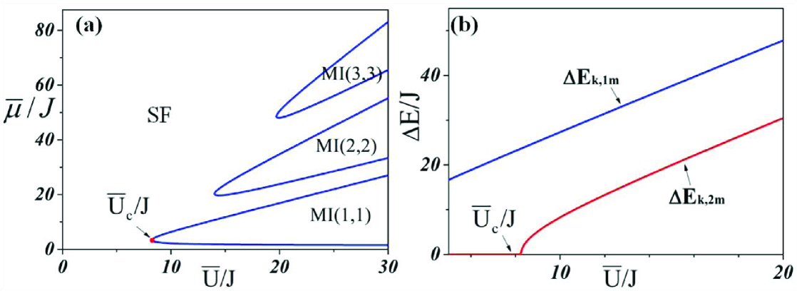
Figure 1: (Color online) (a) Phase diagram of the Bose-Hubbard extension of WSM. The vertical axis and horizontal axis show the dimensionless chemical potential $\bar{\mu}=\mu/z$ and $\bar{U}=U/z$, respectively. (b) The first-order approximations to the dispersion of the density fluctuations.

II.2 Superfluid-Mott insulator transition

After turning on the interaction $U$ ($>0$) between particles, the ground state of the system enters into superfluid (SF) phase with noninteger number of bosons at each site at zero temperature. As interaction increases, qualitatively the interaction between particles will drive the system into Mott insulator (MI) phase if $U\gg t$, in which the moving for a particle from one site to another is energetically unfavorable.

In the strong coupling limit, we first introduce a local superfluid order parameter that is written as van ; lim

$$\psi_{\mathbf{r}}=\langle\hat{a}_{\mathbf{r}}^{{\dagger}}\rangle=\langle\hat{a}_{\mathbf{r}}\rangle.$$ (10)

Owing to that there are two kinds of lattice sites in the model, i.e., $A$-sublattice and $B$-sublattice, we define order parameters as $\psi_{\mathbf{r\in}A}\equiv\psi_{A}$ and $\psi_{\mathbf{r\in}B}\equiv\psi_{B}$, respectively. With the help of $\psi_{\mathbf{r}}$, the hopping terms in Eq. (2) can be decoupled, and in the occupation numbers basis we readily arrive at the per unit cell ground state energy for the system up to the second-order perturbation as

$$E_{g}\left(\psi_{A},\psi_{B}\right) \simeq a_{0}+a_{2}\psi_{A}^{2}+c_{2}\psi_{A}\psi_{B}$$

$$+b_{2}\psi_{B}^{2}+\mathcal{O}\left(\psi_{A}^{4},\psi_{B}^{4}\right).$$ (11)

Here, coefficients $a_{0}$, $a_{2}$, $c_{2}$, and $b_{2}$ are as follows:

$$a_{0}=\frac{\overline{U}}{2}(n_{A}^{2}+n_{B}^{2}-n_{u})-\overline{\mu}n_{u},$$ (12)

$$a_{2} =-J_{z}+\frac{(-\overline{U}-\mu)J_{z}{}^{2}}{\left[(n_{A}-1)\overline{U}-\overline{\mu}\right]\left[-n_{A}\overline{U}+\overline{\mu}\right]}$$

$$+\frac{(-\overline{U}-\overline{\mu})(J_{x}+J_{y})^{2}}{\left[(n_{B}-1)\overline{U}-\overline{\mu}\right]\left[-n_{B}\overline{U}+\overline{\mu}\right]},$$ (13)

$$b_{2} =J_{z}+\frac{(-\overline{U}-\overline{\mu})(J_{x}-J_{y})^{2}}{\left[(n_{A}-1)\overline{U}-\overline{\mu}\right]\left[-n_{B}\overline{U}+\overline{\mu}\right]}$$

$$+\frac{(-\overline{U}-\overline{\mu})J_{z}^{2}}{\left[(n_{B}-1)\overline{U}-\overline{\mu}\right]\left[-n_{B}\overline{U}+\overline{\mu}\right]},$$ (14)

$$c_{2} =2J_{y}+\frac{2(-\overline{U}-\overline{\mu})(J_{x}-J_{y})J_{z}}{\left[(n_{A}-1)\overline{U}-\overline{\mu}\right]\left[-n_{A}\overline{U}+\overline{\mu}\right]},$$

$$+\frac{2(-\overline{U}-\overline{\mu})(J_{x}+J_{y})J_{z}}{\left[(n_{B}-1)\overline{U}-\overline{\mu}\right]\left[-n_{B}\overline{U}+\overline{\mu}\right]},$$ (15)

where $\bar{U}=U/z$, $\bar{\mu}=\bar{\mu}/z$ with $z=2$ being the number of nearest-neighbor sites in one direction, the average particle number in one unit cell $n_{u}=n_{A}+n_{B}$, $n_{A}$ and $n_{B}$ are particle number on $A$- and $B$-sublattice, respectively. See Appendix A for detailed calculations. By means of Landau theory, based on the geometry knowledge, when the Gaussian curvature of the energy-order parameters surface is zero at the point $\psi_{A}=\psi_{B}=0$, the phase transition occurs chenb . Therefore, we can obtain a function of phase-transition line readily by

$$\frac{\partial^{2}E}{\partial\psi_{A}^{2}}|_{\left(0,0\right)}\frac{\partial^{2}E}{\partial\psi_{B}^{2}}|_{\left(0,0\right)}-\left(\frac{\partial^{2}E}{\partial\psi_{A}\partial\psi_{B}}|_{\left(0,0\right)}\right)^{2}=0,$$ (16)

which leads to the function of phase-transition line:

$$4a_{2}b_{2}-c_{2}^{2}=0.$$ (17)

Solving Eq. (17), yields

$$\overline{\mu} =\frac{1}{2}\left[-\sqrt{2}+(2\tilde{n}-1)\overline{U}\right.$$

$$\left.\pm\sqrt{2-2\sqrt{2}\overline{U}-4\sqrt{2}\tilde{n}\overline{U}+\overline{U}^{2}}\right]$$ (18)

with the particle number $\tilde{n}\equiv n_{A}=n_{B}$. Correspondingly, the point of smallest $\bar{U}$ (denoted by $\bar{U}_{c}$) for each lobe is

$$\bar{U}_{c}=\sqrt{2}+2\sqrt{2}\tilde{n}+2\sqrt{2\tilde{n}+2\tilde{n}^{2}}.$$ (19)

In conclusion, by applying the Landau theory of phase transitions that treats the interactions exactly and the hopping terms as perturbation, we get the phase diagram in Fig. 1 (a). It shows that the phase transition occurs at $\bar{U}_{c}/J\approx 8.25$ for the MI $\left(1,1\right)$ lobe with the particle number configuration $\left\{n_{A}=1,n_{B}=1\right\}$.

For the case of $U<U_{c}$, the system is in the SF phase. According to the Hugenholtz-Pines theorem, there are always gapless density fluctuations. In the followings, we will study the excitation modes in SF phase.

III Bogoliubov theory and topology of excitation modes for superfluid

In this section, by using the Bogoliubov theory for homogeneous condensates with weak repulsive interactions, we determine the band structure of Bogoliubov excitations. Here, homogeneous case refers to the situation where the system has the periodicity of the lattice. We then study the topology of Bogoliubov excitations, and determine whether the excitations have novel properties.

By means of the Gross-Pitaevskii (GP) theory, we derive the condensate wave function to formulate the Bogoliubov theory for the boson system. In the GP theory, we first introduce the GP energy function $E$ by replacing $\left(\hat{a}_{\mathbf{r}},\hat{a}_{\mathbf{r}}^{\dagger}\right)$ by $\left(\psi_{\mathbf{r}},\psi_{\mathbf{r}}^{\dagger}\right)$ in the Hamiltonian in Eq. (2), and minimize it with respect to $\left(\psi_{\mathbf{r}},\psi_{\mathbf{r}}^{\dagger}\right)$ under the constraint $\sum_{\mathbf{r}}\left|\psi_{\mathbf{r}}\right|^{2}=N$. Since the single-particle ground state is formed at $\mathbf{k}_{0}$, we first introduce the following homogeneous ansatz for the interacting case: $\psi_{\mathbf{r}}=\frac{1}{\sqrt{N_{uc}}}\psi_{{}_{X}}$ ($X\in A,B$) with $N_{uc}$ being the number of unit cells. Next, we introduce the chemical potential $\mu$ as a Lagrange multiplier to satisfy the particle-number constraint. The functional to be minimized is then given by

$$E-\mu N =\left(\psi_{{}_{A}}^{\ast},\psi_{{}_{B}}^{\ast}\right)\left[\mathcal{H}\left(\mathbf{k}_{0}\right)-\mu I\right]\left(\begin{array}[c]{c}\psi_{{}_{A}}\\ \psi_{{}_{B}}\end{array}\right)$$ (22)

$$+\frac{U}{N_{uc}}\left(\left|\psi_{{}_{A}}\right|^{4}+\left|\psi_{{}_{B}}\right|^{4}\right).$$ (23)

Minimizing $E-\mu N$ with respect to $\psi_{{}_{X}}^{\ast}$ ($X\in A,B$) gives a homogeneous version of the GP equations:

$$\left[\mathcal{H}\left(\mathbf{k}_{0}\right)-\mu I\right]\left(\begin{array}[c]{c}\psi_{{}_{A}}\\ \psi_{{}_{B}}\end{array}\right)+\frac{U}{N_{uc}}\left(\begin{array}[c]{c}\psi_{{}_{A}}^{\ast}\psi_{{}_{A}}^{2}\\ \psi_{{}_{B}}^{\ast}\psi_{{}_{B}}^{2}\end{array}\right)=0.$$ (24)

Since the single-particle ground state is created by $a_{-}^{\dagger}\left(\mathbf{k}_{0}\right)$ in Eq. (8), it is convenient to parameterize $\left(\psi_{{}_{A}},\psi_{{}_{B}}\right)^{T}$ as

$$\left(\begin{array}[c]{c}\psi_{{}_{A}}\\ \psi_{{}_{B}}\end{array}\right)=\sqrt{N}\left(\begin{array}[c]{c}f_{{}_{A}}\\ f_{{}_{B}}\end{array}\right)=\sqrt{N}\left(\begin{array}[c]{c}-e^{-i\varphi}\sin\left(\frac{\theta}{2}\right)\\ \cos\left(\frac{\theta}{2}\right)\end{array}\right),$$ (25)

where $\theta=\theta_{0}$ when $U=0$. Multiplying Eq. (24) by $\left(f_{{}_{A}}^{\ast},f_{{}_{B}}^{\ast}\right)$ or $\left(-f_{{}_{B}}^{\ast},f_{{}_{A}}^{\ast}\right)$ from the left, we get

$$-h\left(\mathbf{k}_{0}\right)\left[\cos\theta_{0}\cos\theta+\sin\theta_{0}\sin\theta\cos\left(\varphi_{0}-\varphi\right)\right]+2Un\left(\left|f_{{}_{A}}\right|^{4}+\left|f_{{}_{B}}\right|^{4}\right) =\mu,$$ (26)

$$h\left(\mathbf{k}_{0}\right)\left(\cos\theta_{0}\sin\theta\cos\varphi-\sin\theta_{0}\cos\varphi_{0}\cos\theta\right)-Un\cos\varphi\sin\theta\cos\theta =0,$$ (27)

$$h\left(\mathbf{k}_{0}\right)\sin\theta_{0}\sin\varphi_{0}+\mu\sin\theta\sin\varphi-Un\sin\theta\sin\varphi =0$$ (28)

where $n=N/\left(2N_{uc}\right)$.

We now discuss excitations from the condensate ground state by using the Bogoliubov theory. Firstly, $\hat{a}_{\mathbf{r}}$ is decomposed into the condensate and noncondensate parts with the help of Fourier transformation as

$$\hat{a}_{\mathbf{r}}=\frac{1}{\sqrt{N_{uc}}}f_{X}\hat{a}_{-}+\tilde{a}_{\mathbf{r}},$$ (29)

where $\tilde{a}_{\mathbf{r}}=\frac{1}{\sqrt{N_{uc}}}\left[-\epsilon_{X}f_{\bar{X}}^{\ast}\hat{a}_{+}+\sum_{\mathbf{k\neq 0}}\hat{a}_{X,\mathbf{k}}e^{i\mathbf{k}.\mathbf{r}}\right]$ with $\bar{A}=B$ and $\bar{B}=A$, $f_{{}_{A}}=-e^{-i\varphi}\sin\left(\frac{\theta}{2}\right)$ and $f_{{}_{B}}=\cos\left(\frac{\theta}{2}\right)$. Following the Bogoliubov approximation, we replace both $\hat{a}_{-}$ and $\hat{a}_{-}^{\dagger}$ by $\sqrt{N}$, and substitute equation (29) into $H-\mu N$ up to quadratic order in $\tilde{a}_{\mathbf{r}}$. The terms linear in $\tilde{a}_{\mathbf{r}}$ or $\tilde{a}_{\mathbf{r}}^{\dagger}$ disappear due to the stability condition of the condensate, and we arrive at the Bogoliubov Hamiltonian as

$$H-\mu N=\frac{1}{2}\mathcal{A}^{\dagger}M_{+}\mathcal{A}+\frac{1}{2}\sum_{\mathbf{k\neq 0}}\hat{\alpha}_{\mathbf{k}}^{\dagger}M\left(\mathbf{k}\right)\hat{\alpha}_{\mathbf{k}}$$ (30)

with $\hat{\alpha}_{\mathbf{k}}^{\dagger}=\left(\hat{a}_{A,\mathbf{k}}^{\dagger},\hat{a}_{B,\mathbf{k}}^{\dagger},\hat{a}_{A,-\mathbf{k}},\hat{a}_{B,-\mathbf{k}}\right)$ and $\mathcal{A}^{\dagger}=\left(\hat{a}_{+}^{\dagger},\hat{a}_{+}\right)$. Here, the $2\times 2$ matrix $M_{+}$ and $4\times 4$ matrix $M\left(\mathbf{k}\right)$ are given by

$$M_{+} =\left\{h\left(\mathbf{k}_{0}\right)\left[\cos\theta_{0}\cos\theta-\sin\theta_{0}\sin\theta\cos\left(\varphi_{0}+\varphi\right)\right]-\mu\right.$$

$$\left.+8Un\left|f_{A}\right|^{2}\left|f_{B}\right|^{2}\right\}I+N_{+},$$ (31)

with $N_{+}=4Un\left[\operatorname{Re}\left(f_{A}^{\ast}f_{B}^{\ast}\right)\sigma_{1}-\operatorname{Im}\left(f_{A}^{\ast}f_{B}^{\ast}\right)\sigma_{2}\right]$, and

$$M\left(\mathbf{k}\right)$$

$$=\left(\begin{array}[c]{cc}\mathcal{H}\left(\mathbf{k}\right)-\mu I+4Un\left|F\right|^{2}&2UnF^{2}\\ 2UnF^{\ast 2}&\mathcal{H}^{T}\left(-\mathbf{k}\right)-\mu I+4Un\left|F\right|^{2}\end{array}\right).$$ (34)

where $F=\mathrm{diag}\left(f_{A},f_{B}\right)$.

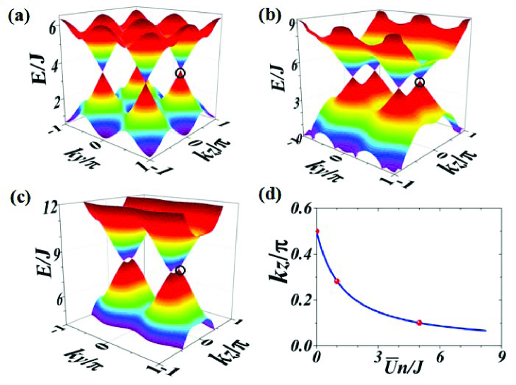
Figure 2: (Color online) The energy spectra of Bogoliubov quasiparticles with fixed $k_{x}=0$ and (a) $\overline{U}n/J=0.0$; (b) $\overline{U}n/J=1.0$; (c) $\overline{U}n/J=5.0$. (d) The $k_{z}$-coordinates of Weyl points versus $\overline{U}n$, of which the ones indicated by black circles in (a), (b), (c) are indicated by red points.

To diagonalize above Bogoliubov Hamiltonian, we introduce paraunitary matrices $W_{+}$ and $W_{\mathbf{k}}$ which satisfy $W_{+}^{\dagger}\sigma_{3}W_{+}=W_{+}\sigma_{3}W_{+}^{\dagger}=\sigma_{3}$, and $W_{\mathbf{k}}^{\dagger}\tau_{3}W_{\mathbf{k}}=W_{\mathbf{k}}\tau_{3}W_{\mathbf{k}}^{\dagger}=\tau_{3}$ with $\sigma_{3}=\mathrm{diag}\left(1,-1\right)$ and $\tau_{3}=\mathrm{diag}\left(1,1,-1,-1\right)$ Fur ; col , and then obtain

$$W_{+}^{\dagger}M_{+}W_{+}=E_{+}\left(0\right)I,$$ (35)

$$W_{\mathbf{k}}^{\dagger}M\left(\mathbf{k}\right)W_{\mathbf{k}}=\mathrm{diag}\left(E_{+,\mathbf{k}},E_{-,\mathbf{k}},E_{+,-\mathbf{k}},E_{-,-\mathbf{k}}\right).$$ (36)

See Appendix B for details. At last, the Hamiltonian in Eq. (30) is diagonalized as

$$H-\mu N=\sum_{\mathbf{k}}E_{+,\mathbf{k}}\hat{b}_{+,\mathbf{k}}^{\dagger}\hat{b}_{+,\mathbf{k}}+\sum_{\mathbf{k\neq 0}}E_{-,\mathbf{k}}\hat{b}_{-,\mathbf{k}}^{\dagger}\hat{b}_{-,\mathbf{k}}+const.$$ (37)

By direct numerical calculations, we get the Bogoliubov excitation bands $E_{\pm,\mathbf{k}}$ as shown in Fig. 2. It shows that there are Weyl points in the excitation band. As the interaction strength increases, Weyl points approach gradually with each other along the $k_{z}$-direction (see Fig. 2 (d)).

To study the topological properties of excitation modes of Bogoliubov quasiparticles, we define the basis vectors of $M\left(\mathbf{k}\right)$ as $\left|w_{\lambda}\left(\mathbf{k}\right)\right\rangle=\left(\alpha_{A,\lambda}\left(\mathbf{k}\right),\alpha_{B,\lambda}\left(\mathbf{k}\right),\beta_{A,\lambda}\left(\mathbf{k}\right),\beta_{B,\lambda}\left(\mathbf{k}\right)\right)^{T}$ with $\lambda=\pm$, of which $\left\langle w_{\lambda^{\prime}}\left(\mathbf{k}\right)\right|\tau_{3}\left|w_{\lambda}\left(\mathbf{k}\right)\right\rangle=\delta_{\lambda^{\prime}\lambda}$. We then have $M\left(\mathbf{k}\right)\left|w_{\lambda}\left(\mathbf{k}\right)\right\rangle=E_{\lambda}\left(\mathbf{k}\right)\tau_{3}\left|w_{\lambda}\left(\mathbf{k}\right)\right\rangle$, and the Berry curvature takes the form as

$$B_{\lambda,k}\left(\mathbf{k}\right)=i\epsilon_{ijk}\left\langle\partial_{i}w_{\lambda}\left(\mathbf{k}\right)\left|\tau_{3}\right|\partial_{j}w_{\lambda}\left(\mathbf{k}\right)\right\rangle$$ (38)

with $\partial_{j}\equiv\partial/\partial k_{j}$ and $j=x$, $y$, $z$. The topology of Weyl point is characterized by the first Chern number defined by $C_{\mathbf{k}_{w},-}={\displaystyle\oint}d\mathbf{S\cdot B}_{-}\left(\mathbf{k}\right)$, which is calculated by the integral of Berry curvature throughout the surface enclosing the Weyl point. After direct calculations, we obtain $C_{\mathbf{k}_{w},-}=\pm 1$ which implies that Weyl points have different chiralities. It shows a synthetic magnetic monopole located at $\left\{\mathbf{k}_{w}\right\}$.

We apply the BdG theory to study the Bogoliubov excitations of superfluids by choosing a slab with finite width along planes orthogonal to the $\vec{x}-\vec{y}$ direction, which has sharp the boundaries. The energy spectra and contour plot of upper energy spectra of excitation modes are shown in Fig. 3(a) and (b), respectively. There are topologically protected surface states (dubbed bosonic arcs) of excitation modes which are the analogs of Fermi arcs in electronic systems. As the interaction increases, two arcs connected by two Weyl points will approach gradually with each other along the $k_{z}$-direction.

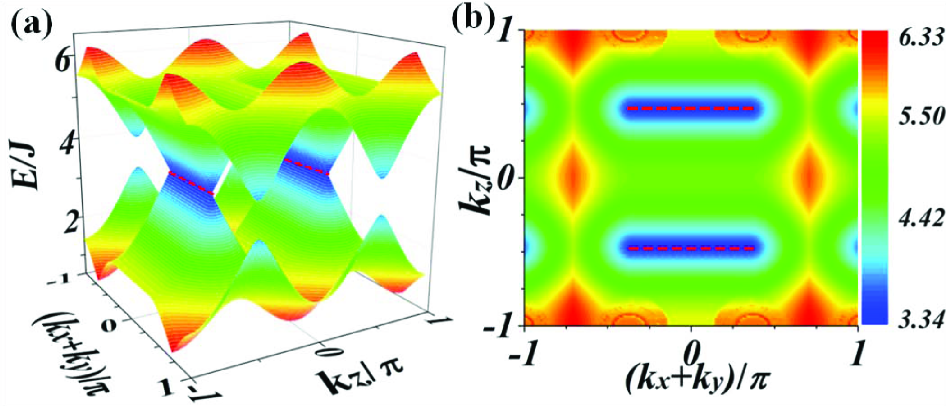
Figure 3: (Color online) (a) The Bogoliubov spectra of slab with finite width. The bosonic surface-arc states are indicated by red dashed lines. (b) The contour plot of upper energy spectra of excitation modes for BECs in a slab with finite width along planes orthogonal to the $\vec{x}-\vec{y}$ direction. The arc states are indicated by red dashed lines. In both (a) and (b), the parameter $\bar{U}n/J=0.2$.

IV Excitations in Mott insulator phase

In the strong coupling regime, we apply the path integral formulation to calculate the excitation spectra of the MI state lim . We first write the partition function for the Bose-Hubbard extension in terms of path integral as $Z={\displaystyle\int}\mathcal{D}a^{\ast}\mathcal{D}a\exp\left\{-S\left[a^{\ast},a\right]/\hbar\right\}$, where the action is given by

$$S\left[a^{\ast},a\right] ={\displaystyle\int_{0}^{\beta}}d\tau\left[{\displaystyle\sum\limits_{\mathbf{r}}}a_{\mathbf{r}}^{\ast}\left(\tau\right)(\hbar\partial_{\tau}-\mu)a_{\mathbf{r}}\left(\tau\right)+H_{0}\left(\tau\right)\right.$$

$$\left.+\frac{1}{2}U{\displaystyle\sum\limits_{\mathbf{r}}}a_{\mathbf{r}}^{\ast}\left(\tau\right)a_{\mathbf{r}}^{\ast}\left(\tau\right)a_{\mathbf{r}}\left(\tau\right)a_{\mathbf{r}}\left(\tau\right)\right]$$ (39)

with $\beta=\frac{1}{k_{B}T}$, $k_{B}$ is the Boltzman constant, and $H_{0}\left(\tau\right)$ is obtained by replacing the bosonic operators $\left(\hat{a}_{\mathbf{r}}^{\dagger}\text{, }\hat{a}_{\mathbf{r}}\right)$ in Eq. (2) by complex functions $\left(a_{\mathbf{r}}^{\ast}\left(\tau\right)\text{, }a_{\mathbf{r}}\left(\tau\right)\right)$. To decouple the hopping terms, we make use of Hubbard-Stratonovich transformation and rewrite the action as lim

$$S\left[a^{\ast},a,\psi^{\ast},\psi\right]=S\left[a^{\ast},a\right]+\int_{0}^{\hbar\beta}d\tau{\displaystyle\sum\limits_{\mathbf{r,j}}}(\psi_{\mathbf{r}}^{\ast}-a_{\mathbf{r}}^{\ast})J_{\mathbf{rj}}(\psi_{\mathbf{j}}-a_{\mathbf{j}}),$$ (40)

where $\psi_{\mathbf{r}}^{\ast}$ and $\psi_{\mathbf{j}}$ are the order parameter fields, and $J_{\mathbf{rj}}$ denotes real nearest-neighbor hopping parameters along the $x$, $y$, and $z$ direction. By performing integration over the complex fields $a_{\mathbf{r}}^{\ast}$ and $a_{\mathbf{r}}$, and after direct calculations, we get the effective action up to the second order near the phase transition point as

$$S^{eff}\left[\psi^{\ast},\psi\right] ={\displaystyle\sum\limits_{\mathbf{k},\omega_{m}}}\Psi_{\mathbf{k},\omega_{m}}^{\ast}(\mathcal{H}\left(\mathbf{k}\right)\mathcal{-H}\left(\mathbf{k}\right)^{2}f_{\omega_{m}})\Psi_{\mathbf{k},\omega_{m}}$$

$$={\displaystyle\sum\limits_{\mathbf{k},\omega_{m}}}\Psi_{\mathbf{k},\omega_{m}}^{\ast}\left[-\hbar G^{-1}(\mathbf{k},i\omega_{m})\right]\Psi_{\mathbf{k},\omega_{m}},$$ (41)

where $\Psi_{\mathbf{k},\omega_{m}}^{\ast}=\left(\psi_{A\mathbf{k},\omega_{m}}^{\ast}\text{, }\psi_{B\mathbf{k},\omega_{m}}^{\ast}\right)$, and

$$f_{\omega_{m}}=\frac{\tilde{n}+1}{-i\hbar\omega_{m}-\mu+\tilde{n}U}+\frac{\tilde{n}}{i\hbar\omega_{m}+\mu-(\tilde{n}-1)U}.$$ (42)

See Appendix C for detailed calculations.

Under the usual analytic continuation $i\omega_{m}\rightarrow\omega_{m}$, we can obtain a function of real energies $\hbar\omega$, i.e.,

$$\det\left[G^{-1}\left(\mathbf{k},i\omega_{m}\right)\right]=0.$$ (43)

The quasiparticle- and quasihole-dispersion relations are obtained as

$$\hbar\omega_{1,qp,ph} =\frac{1}{2}\left[-2\mu+(2\tilde{n}-1)U-\frac{1}{f_{\omega_{m_{+}}}}\pm\Delta E_{\mathbf{k}1}\right],$$

$$\hbar\omega_{2,qp,ph} =\frac{1}{2}\left[-2\mu+(2\tilde{n}-1)U-\frac{1}{f_{\omega_{m_{-}}}}\pm\Delta E_{\mathbf{k}2}\right],$$ (44)

where $\Delta E_{\mathbf{k},1}=\sqrt{U^{2}-\frac{(4\tilde{n}+2)U}{f_{\omega_{m_{+}}}}+\frac{1}{f_{\omega_{m_{+}}}^{2}}}$, $\Delta E_{\mathbf{k},2}=\sqrt{U^{2}-\frac{(4\tilde{n}+2)U}{f_{\omega_{m_{-}}}}+\frac{1}{f_{\omega_{m_{-}}}^{2}}}$, $f_{\omega_{m_{\pm}}}=\frac{A+B\pm\sqrt{(A-B)^{2}+4C^{\ast}C}}{2(AB-C^{\ast}C)}$, $A=-B=2J_{z}\cos(k_{z})$ and $C=-2J_{y}\cos(k_{y})+i2J_{x}\sin(k_{x})$. See quasiparticle- and quasihole-dispersions in Fig. 4 (a) and (b). In addition, we also plot the first-order approximations (the minimum values of $\Delta E_{\mathbf{k},1}$ and $\Delta E_{\mathbf{k},2}$, i.e., $\Delta E_{\mathbf{k},1m}$ and $\Delta E_{\mathbf{k},2m}$) to the dispersion of the density fluctuations in Fig. 1 (b). Fig. 1 (b) indicates that the band gap disappears as we approach the critical value $\bar{U}_{c}/J\approx 8.25$ that is consistent with the result found in Fig. 1 (a). Fig. 4 (a) and (b) also show that there are Weyl nodes in the Bogoliubov excitation spectra in Mott-insulator phase, and the Mott gap $E_{\mathbf{k},2m}$ becomes larger as the interaction strength increases similar to that in conventional Bose-Hubbard models.

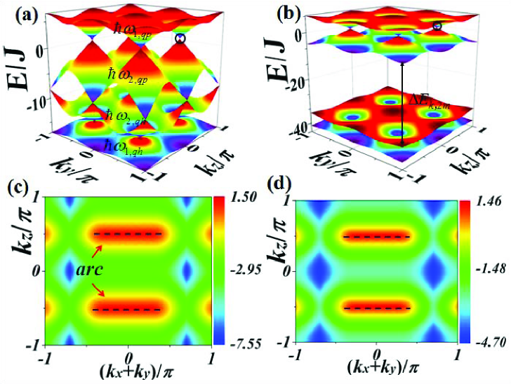
Figure 4: (Color online) The energy spectra of quasiparticle and quasihole excitations with fixed $k_{x}=0$ for (a) $\bar{U}/J=8.25$ and (b) $\bar{U}/J=20.0$ in MI$(1,1)$ phase; and the contour plot of energy spectra of lower one of quasiparticle-excitation modes in MI$(1,1)$ phase in a slab with finite width along planes orthogonal to the $\vec{x}-\vec{y}$ direction for (c) $\bar{U}/J=8.25$ and (d) $\bar{U}/J=20.0$ in MI$(1,1)$ phase. The locations of the Weyl nodes are shown indicated by black circles in (a) and (b). The bosonic arc states are indicated by black dashed lines in (c) and (d).

Next, we apply the BdG theory to study the quasiparticle and quasihole excitations in Mott-insulator phase by choosing a slab with finite width and the sharp boundaries along planes orthogonal to the $\vec{x}-\vec{y}$ direction. After calculations, we present the results in Fig. 4 (c) and (d), which show that there are also bosonic surface-arc states at boundaries.

V Discussion and Conclusion

The Hamiltonian of WSM in Eq. (2) in three-dimensional optical lattices has been proposed by using laser-assisted tunneling in Ref. ten . The interaction between particles may be tuned readily by using Feshbach resonance technique. To experimentally measure the topological properties of the elementary Bogoliubov excitations in SF phase, one may coherently transfer a small portion of the condensate into a surface mode by stimulated Raman transitions ern ; zhi . Owing to that the original bosons and the Bogoliubov excitations is connected by the paraunitary matrix, a density wave may form from the interference of the surface modes and the condensate wave function by the mechanism discussed in Ref. Fur .

In summary, Bogoliubov excitations in Bose-Hubbard extension of the WSM are studied. By using Bogoliubov theory, we calculate the energy spectra of excitation modes for the system with weak repulsive interactions, and find their non-trivial properties owing to the existence of Weyl points. There exist bosonic surface-arcs connected by Weyl points with different chiralities analogs of Fermi arc in WSM of electronic system. As the interaction increases, Weyl points approach gradually with each other along the $k_{z}$-direction. In the strong coupling regime, the system is in MI phase. By using path integral formulation, we find that there are two quasiparticle dispersions touching at stable nodes (Weyl points), and there are also bosonic surface-arc at boundaries.

In addition to the type-I WSM considered in this paper, we expect that there are also novel excitations in the Bose-Hubbard extension of type-II xu1 ; sol ; xu2 and hybrid WSMs li ; kong . The bosonic Weyl excitations will deepen our standing of quantum many body physics in boson systems.

Appendix A Landau theory for superfluid-Mott insulator transition

In the strong coupling limit, we first introduce a local superfluid order parameter given by van ; lim

$$\psi_{\mathbf{r}}=\langle\hat{a}_{\mathbf{r}}^{{\dagger}}\rangle=\langle\hat{a}_{\mathbf{r}}\rangle.$$ (45)

Due to $A$-sublattice and $B$-sublattice for the lattice system, the order parameters are defined as $\psi_{\mathbf{r\in}A}\equiv\psi_{A}$, $\psi_{\mathbf{r\in}B}\equiv\psi_{B}$, $n_{\mathbf{r\in}A}\equiv n_{A}$ and $n_{\mathbf{r\in}B}\equiv n_{B}$, respectively. With the help of $\psi_{\mathbf{r}}$, we decouple the hopping term into

$$\hat{a}_{\mathbf{r}}^{{\dagger}}\hat{a}_{\mathbf{j}}=\hat{a}_{\mathbf{r}}^{{\dagger}}\psi_{\mathbf{j}}+\psi_{\mathbf{r}}\hat{a}_{\mathbf{j}}-\psi_{\mathbf{r}}\psi_{\mathbf{j}},$$ (46)

where $\mathbf{j}$ denotes the coordinate of lattice site $\mathbf{r}$’s nearest neighbor site. Then the Hamiltonian takes following form:

$$\hat{H}^{eff} =\sum_{\mathbf{r}\in B}\left[-J_{x}(\hat{a}_{\mathbf{r}}+\hat{a}_{\mathbf{r}}^{{\dagger}}-\psi_{\mathbf{r}})\psi_{\mathbf{r}+\mathbf{\delta}_{x}}\right.$$

$$\left.-J_{y}(\hat{a}_{\mathbf{r}}+\hat{a}_{\mathbf{r}}^{{\dagger}}-\psi_{\mathbf{r}})\psi_{\mathbf{r}+\mathbf{\delta}_{y}}-J_{z}(\hat{a}_{\mathbf{r}}+\hat{a}_{\mathbf{r}}^{{\dagger}}-\psi_{\mathbf{r}})\psi_{\mathbf{r}+\mathbf{\delta}_{z}})\right]$$

$$+\sum_{\mathbf{r}\in A}\left[J_{x}(\hat{a}_{\mathbf{r}}+\hat{a}_{\mathbf{r}}^{{\dagger}}-\psi_{\mathbf{r}})\psi_{\mathbf{r}+\mathbf{\delta}_{x}}\right.$$

$$\left.-J_{y}(\hat{a}_{\mathbf{r}}+\hat{a}_{\mathbf{r}}^{{\dagger}}-\psi_{\mathbf{r}})\psi_{\mathbf{r}+\mathbf{\delta}_{y}}+J_{z}(\hat{a}_{\mathbf{r}}+\hat{a}_{\mathbf{r}}^{{\dagger}}-\psi_{\mathbf{r}})\psi_{\mathbf{r}+\mathbf{\delta}_{z}})\right]$$

$$+\frac{U}{2}\sum_{\mathbf{r}}n_{\mathbf{r}}(n_{\mathbf{r}}-1)-\mu\sum_{\mathbf{r}}\hat{a}_{\mathbf{r}}^{{\dagger}}\hat{a}_{\mathbf{r}}.$$ (47)

For the system, the effective onsite Hamiltonian $\hat{H}_{on}^{eff}$ is then given by

$$\hat{H}_{on}^{eff} =J_{x}(\hat{a}_{A}^{{\dagger}}+\hat{a}_{A})\psi_{B}-J_{x}(\hat{a}_{B}^{{\dagger}}+\hat{a}_{B})\psi_{1}$$

$$-J_{y}(\hat{a}_{A}^{{\dagger}}+\hat{a}_{A})\psi_{B}-J_{y}(\hat{a}_{B}^{{\dagger}}+\hat{a}_{B})\psi_{A}+2J_{y}\psi_{A}\psi_{B}$$

$$+J_{z}(\hat{a}_{A}^{{\dagger}}+\hat{a}_{A})\psi_{A}-J_{z}(\hat{a}_{B}^{{\dagger}}+\hat{a}_{B})\psi_{B}$$

$$+J_{z}(\psi_{B}^{2}-\psi_{A}^{2})+\frac{\overline{U}}{2}(n_{A}^{2}+n_{B}^{2}-n_{u})-\overline{\mu}n_{u}$$ (48)

where $\bar{U}=U/z$, and $\bar{\mu}=\bar{\mu}/z$, and $z=2$ is the number of nearest-neighbor sites in one direction. Next, we write $\hat{H}_{on}=\hat{H}_{on}^{0}+\hat{H}_{on}^{{}^{\prime}}$ with

$$\hat{H}_{on}^{0} =\frac{\overline{U}}{2}(n_{A}^{2}+n_{B}^{2}-n_{u})-\overline{\mu}n_{u}$$

$$+2J_{y}\psi_{A}\psi_{B}+J_{z}(\psi_{B}^{2}-\psi_{A}^{2})$$ (49)

and

$$\hat{H}_{on}^{\prime} =J_{x}(\hat{a}_{A}^{{\dagger}}+\hat{a}_{A})\psi_{B}-J_{x}(\hat{a}_{B}^{{\dagger}}+\hat{a}_{B})\psi_{A}$$

$$-J_{y}(\hat{a}_{A}^{{\dagger}}+\hat{a}_{A})\psi_{B}-J_{y}(\hat{a}_{B}^{{\dagger}}+\hat{a}_{B})\psi_{A}$$

$$+J_{z}(\hat{a}_{A}^{{\dagger}}+\hat{a}_{A})\psi_{A}-J_{z}(\hat{a}_{B}^{{\dagger}}+\hat{a}_{B})\psi_{B}.$$ (50)

In the occupation numbers basis, we can find that the odd powers of the expansion of energy are always zero. Hence, the energy for the zero-order terms is then given by

$$E_{g}^{(0)} =\min(e_{\{n_{A};n_{B}\}}^{(0)})$$

$$=\frac{\overline{U}}{2}(n_{A}^{2}+n_{B}^{2}-n_{u})-\overline{\mu}n_{u}$$

$$+2J_{y}\psi_{A}\psi_{B}+J_{z}(\psi_{B}^{2}-\psi_{A}^{2}),$$ (51)

and the energy for the second-order perturbation is

$$E_{g}^{(2)}=\frac{\left\langle n_{A};n_{B}\left|H_{on}^{{}^{\prime}}\right|k_{1};k_{2}\right\rangle\left\langle k_{1};k_{2}\left|H_{on}^{{}^{\prime}}\right|n_{A};n_{B}\right\rangle}{E_{g}^{(0)}-E_{k}^{(0)}},$$ (52)

where $k_{1}=n_{A}+1$, $k_{2}=n_{B}$ or $k_{1}=n_{A}$, $k_{2}=n_{B}+1$. After direct calculations, we obtain

$$E_{g}^{(2)} =\frac{n_{A}(J_{x}\psi_{B}-J_{y}\psi_{B}+J_{z}\psi_{A})^{2}}{(n_{A}-1)\overline{U}-\overline{\mu}}$$

$$+\frac{(n_{A}+1)(J_{x}\psi_{B}-J_{y}\psi_{B}+J_{z}\psi_{A})^{2}}{-n_{A}\overline{U}+\overline{\mu}}$$

$$+\frac{n_{B}(-J_{x}\psi_{A}-J_{y}\psi_{A}-J_{z}\psi_{B})^{2}}{(n_{B}-1)\overline{U}-\overline{\mu}}$$

$$+\frac{(n_{B}+1)(-J_{x}\psi_{A}-J_{y}\psi_{A}-J_{z}\psi_{B})^{2}}{-n_{B}\overline{U}+\overline{\mu}}$$ (53)

In summary, the per unit cell ground-state energy for the system in terms of $\left(\psi_{A},\psi_{B}\right)$ is given by

$$E_{g} \simeq E_{g}^{(0)}+E_{g}^{(2)}+...$$

$$=a_{0}+a_{2}\psi_{A}^{2}+c_{2}\psi_{A}\psi_{B}+b_{2}\psi_{B}^{2}+\mathcal{O}\left(\psi_{A}^{4},\psi_{B}^{4}\right),$$ (54)

where the coefficients $a_{0}$, $a_{2}$, $c_{2}$, and $b_{2}$ are listed in Eqs. (12)-(15).

Appendix B Diagonalization of Bogoliubov Hamiltonian for bosons

To diagonalize Bogoliubov Hamiltonian in Eq. (30), we perform generalized Bogoliubov transformations as

$$\left(\begin{array}[c]{c}\hat{a}_{+}\\ \hat{a}_{+}^{\dagger}\end{array}\right)=W_{+}\left(\begin{array}[c]{c}\hat{b}_{+}\left(0\right)\\ \hat{b}_{+}^{\dagger}\left(0\right)\end{array}\right),\hat{\alpha}_{\mathbf{k}}=W\left(\mathbf{k}\right)\hat{\beta}_{\mathbf{k}}$$ (55)

with

$$\hat{\beta}_{\mathbf{k}}^{\dagger}=\left(\hat{b}_{+,\mathbf{k}}^{\dagger},\hat{b}_{-,\mathbf{k}}^{\dagger},\hat{b}_{+,-\mathbf{k}},\hat{b}_{-,-\mathbf{k}}\right).$$

Here, $W_{+}$ and $W_{\mathbf{k}}$ are paraunitary matrices that satisfy following conditions:

$$W_{+}^{\dagger}\sigma_{3}W_{+} =W_{+}\sigma_{3}W_{+}^{\dagger}=\sigma_{3},$$

$$W_{\mathbf{k}}^{\dagger}\tau_{3}W_{\mathbf{k}} =W_{\mathbf{k}}\tau_{3}W_{\mathbf{k}}^{\dagger}=\tau_{3},$$ (56)

where $\sigma_{3}=\mathrm{diag}\left(1,-1\right)$ and $\tau_{3}=\mathrm{diag}\left(1,1,-1,-1\right)$. The $4\times 4$ paraunitary matrix $W_{\mathbf{k}}$ can be constructed numerically, which is written as

$$W_{\mathbf{k}}=\left(\begin{array}[c]{cc}U\left(\mathbf{k}\right)&V^{\ast}\left(-\mathbf{k}\right)\\ V\left(\mathbf{k}\right)&U^{\ast}\left(-\mathbf{k}\right)\end{array}\right),$$ (57)

where

$$U\left(\mathbf{k}\right)=\left(\begin{array}[c]{cc}\alpha_{A,+}\left(\mathbf{k}\right)&\alpha_{A,-}\left(\mathbf{k}\right)\\ \alpha_{B,+}\left(\mathbf{k}\right)&\alpha_{B,-}\left(\mathbf{k}\right)\end{array}\right),$$ (58)

and

$$V\left(\mathbf{k}\right)=\left(\begin{array}[c]{cc}\beta_{A,+}\left(\mathbf{k}\right)&\beta_{A,-}\left(\mathbf{k}\right)\\ \beta_{B,+}\left(\mathbf{k}\right)&\beta_{B,-}\left(\mathbf{k}\right)\end{array}\right).$$ (59)

The transformations with $W_{+}$ and $W_{\mathbf{k}}$ ensure the invariance of the bosonic commutation relations for Bogoliubov excitations. With the help of them, we may diagonalize the Bogoliubov Hamiltonian in Eq. (30) readily, and at last arrive at Eq. (37).

Appendix C Collective modes in MI phase

The partition function for the Bose-Hubbard extension in terms of path integral is written as $Z={\displaystyle\int}\mathcal{D}a^{\ast}\mathcal{D}a\exp\left\{-S\left[a^{\ast},a\right]/\hbar\right\}$, where the action is shown in Eq. (39). For convenience, in the following, we denote $H_{0}\left(\tau\right)$ (hopping terms) as $\sum_{\mathbf{r,j}}J_{\mathbf{rj}}a_{\mathbf{r}}^{\ast}a_{\mathbf{j}}$ that are perturbation terms in strong coupling regime, where $J_{\mathbf{rj}}$ denotes real nearest-neighbor hopping parameters along the $x$, $y$, and $z$ direction. By using Hubbard-Stratonovich transformation, we obtain the action as shown in Eq. (40). After direct calculations, the action becomes

$$S\left[a^{\ast},a,\psi^{\ast},\psi\right] =\int_{0}^{\hbar\beta}d\tau\left[{\displaystyle\sum\limits_{\mathbf{r}}}a_{\mathbf{r}}^{\ast}(\hbar\frac{\partial}{\partial\tau}-\mu)a_{\mathbf{r}}+\frac{1}{2}U{\displaystyle\sum\limits_{\mathbf{r}}}a_{\mathbf{r}}^{\ast 2}\right.$$

$$\left.\times a_{\mathbf{r}}^{2}-{\displaystyle\sum\limits_{\mathbf{r,j}}}J_{\mathbf{rj}}(a_{\mathbf{r}}^{\ast}\psi_{\mathbf{j}}+\psi_{\mathbf{r}}^{\ast}a_{\mathbf{j}})+{\displaystyle\sum\limits_{\mathbf{r,j}}}J_{\mathbf{rj}}\psi_{\mathbf{r}}^{\ast}\psi_{\mathbf{j}}\right].$$ (60)

Then, we have the explicit form as follows:

$$e^{-S^{eff\left[\psi^{\ast},\psi\right]}} =\exp\left(-\frac{1}{\hbar}\int_{0}^{\hbar\beta}d\tau{\displaystyle\sum\limits_{\mathbf{r,j}}}J_{\mathbf{rj}}\psi_{\mathbf{r}}^{\ast}(\tau)\psi_{\mathbf{j}}(\tau)\right)$$

$$\times {\displaystyle\int}\mathcal{D}a^{\ast}\mathcal{D}a\exp\left\{-S^{(0)}\left[a^{\ast},a\right]/\hbar-\frac{1}{\hbar}\int_{0}^{\hbar\beta}d\tau\left(-{\displaystyle\sum\limits_{\mathbf{r,j}}}J_{\mathbf{rj}}(a_{\mathbf{r}}^{\ast}(\tau)\psi_{\mathbf{j}}(\tau)+\psi_{\mathbf{r}}^{\ast}(\tau)a_{\mathbf{j}}(\tau))\right)\right\},$$ (61)

where we have denoted the action for $J_{\mathbf{rj}}=0$ by $S^{(0)}\left[a^{\ast},a\right]$.

Now by using the relation $\left\langle e^{A_{i}}\right\rangle=e^{\left\langle A_{i}\right\rangle+\frac{1}{2}(\left\langle A_{i}^{2}\right\rangle-\left\langle A_{i}\right\rangle^{2})+...}$, we can get the expression for the action $S^{eff}\left[\psi^{\ast},\psi\right]$ up to the second order, i.e.,

$$S^{eff}\left[\psi^{\ast},\psi\right]\approx S^{(0)}\left[\psi^{\ast},\psi\right]+S^{(2)}\left[\psi^{\ast},\psi\right],$$

where $S^{(2)}\left[\psi^{\ast},\psi\right]$ is given by

$$S^{(2)}\left[\psi^{\ast},\psi\right] =\int_{0}^{\hbar\beta}d\tau{\displaystyle\sum\limits_{\mathbf{r,j}}}J_{\mathbf{rj}}\psi_{\mathbf{r}}^{\ast}(\tau)\psi_{\mathbf{j}}(\tau)-\frac{1}{2\hbar}\left\langle\left(\int_{0}^{\hbar\beta}d\tau{\displaystyle\sum\limits_{\mathbf{r,j}}}J_{\mathbf{rj}}\left[a_{\mathbf{r}}^{\ast}(\tau)\psi_{\mathbf{j}}(\tau)+\psi_{\mathbf{r}}^{\ast}(\tau)a_{\mathbf{j}}(\tau)\right]\right)^{2}\right\rangle_{S^{(0)}}$$

$$=-\frac{1}{2\hbar}\left\langle\int_{0}^{\hbar\beta}\int_{0}^{\hbar\beta}d\tau d\tau^{{}^{\prime}}{\displaystyle\sum\limits_{\mathbf{r,j},\mathbf{r}^{\prime}\mathbf{,j}^{\prime}}}J_{\mathbf{rj}}J_{\mathbf{r}^{\prime}\mathbf{j}^{\prime}}\left[a_{\mathbf{r}}^{\ast}(\tau)\psi_{\mathbf{j}}(\tau)+\psi_{\mathbf{r}}^{\ast}(\tau)a_{\mathbf{j}}(\tau)\right]\left[a_{\mathbf{r}^{{}^{\prime}}}^{\ast}(\tau^{{}^{\prime}})\psi_{\mathbf{j}^{{}^{\prime}}}(\tau^{{}^{\prime}})+\psi_{\mathbf{r}^{{}^{\prime}}}^{\ast}(\tau^{{}^{\prime}})b_{\mathbf{j}^{{}^{\prime}}}(\tau^{{}^{\prime}})\right]\right\rangle_{S^{(0)}}$$

$$+\int_{0}^{\hbar\beta}d\tau{\displaystyle\sum\limits_{\mathbf{r,j}}}J_{\mathbf{rj}}\psi_{\mathbf{r}}^{\ast}(\tau)\psi_{\mathbf{j}}(\tau).$$ (62)

According to the correlations, i.e., $\left\langle a_{\mathbf{r}}^{\ast}a_{\mathbf{j}}^{\ast}\right\rangle_{S^{(0)}}=\left\langle a_{\mathbf{r}}a_{\mathbf{j}}\right\rangle_{S^{(0)}}=0$ and $\left\langle a_{\mathbf{r}}^{\ast}a_{\mathbf{j}}\right\rangle_{S^{(0)}}=\left\langle a_{\mathbf{r}}a_{\mathbf{j}}^{\ast}\right\rangle_{S^{(0)}}=\left\langle a_{\mathbf{r}}a_{\mathbf{j}}^{\ast}\right\rangle_{S^{(0)}}\delta_{\mathbf{rj}}$, we have the action $S^{(2)}\left[\psi^{\ast},\psi\right]$, i.e.,

$$S^{(2)}\left[\psi^{\ast},\psi\right]=\int_{0}^{\hbar\beta}d\tau{\displaystyle\sum\limits_{\mathbf{rj}}}\psi_{\mathbf{r}}^{\ast}J_{\mathbf{rj}}\psi_{\mathbf{j}}-\frac{1}{\hbar}\int_{0}^{\hbar\beta}\int_{0}^{\hbar\beta}d\tau d\tau^{{}^{\prime}}{\displaystyle\sum\limits_{\mathbf{r,j},\mathbf{r}^{\prime}\mathbf{,j}^{\prime}}}J_{\mathbf{rj}}J_{\mathbf{r}^{\prime}\mathbf{j}^{\prime}}\psi_{\mathbf{j}}^{\ast}(\tau)\left\langle T_{\tau}\left[a_{\mathbf{r}}(\tau)a_{\mathbf{r}^{{}^{\prime}}}^{\ast}(\tau^{{}^{\prime}})\right]\right\rangle_{S^{(0)}}\psi_{\mathbf{j}^{{}^{\prime}}}(\tau^{{}^{\prime}}).$$ (63)

For the quadratic term, we can get the formulation in momentum space by using Flourier transformation, i.e.,

$${\displaystyle\sum\limits_{ijj^{{}^{\prime}}}}t_{ij}t_{ij^{{}^{\prime}}}\psi_{j}^{\ast}(\tau)\psi_{j^{{}^{\prime}}}(\tau^{{}^{\prime}})={\displaystyle\sum\limits_{\mathbf{k}}}\Psi_{\mathbf{k}}^{\ast}\left(\tau\right)\mathcal{H}\left(\mathbf{k}\right)^{2}\Psi_{\mathbf{k}}^{\ast}\left(\tau^{\prime}\right),$$ (64)

where $\Psi_{\mathbf{k}}^{\ast}\left(\tau\right)=(\psi_{A\mathbf{k}}^{\ast}(\tau),\psi_{B\mathbf{k}}^{\ast}(\tau))$, and the Hamiltonian matrix in Eq. (4) is re-written as

$$\mathcal{H}\left(\mathbf{k}\right)=\left(\begin{array}[c]{cc}A&C^{\ast}\\ C&B\end{array}\right)$$ (65)

with $A=-B=2J_{z}\cos(k_{z})$ and $C=-2J_{y}\cos(k_{y})+i2J_{x}\sin(k_{x})$. Near the phase transformation point, the zero-order effective action $S^{(0)}$ is going to zero. Therefore, the effective action becomes

$$S^{eff} =\int_{0}^{\hbar\beta}{\displaystyle\sum\limits_{k}}\Psi_{\mathbf{k}}^{\ast}\left(\tau\right)\mathcal{H}\Psi_{\mathbf{k}}\left(\tau^{\prime}\right)$$

$$-\frac{1}{\hbar}\int_{0}^{\hbar\beta}\int_{0}^{\hbar\beta}d\tau d\tau^{{}^{\prime}}\left\langle a_{\mathbf{r}}(\tau)a_{\mathbf{r}^{{}^{\prime}}}^{\ast}(\tau^{{}^{\prime}})\right\rangle{\displaystyle\sum\limits_{\mathbf{k}}}\Psi_{\mathbf{k}}^{\ast}\mathcal{H}^{2}\Psi_{\mathbf{k}}$$ (66)

with $\left\langle a_{\mathbf{r}}(\tau)a_{\mathbf{r}^{{}^{\prime}}}^{\ast}(\tau^{{}^{\prime}})\right\rangle_{S^{(0)}}=\left\langle T_{\tau}\left[a_{\mathbf{r}}(\tau)a_{\mathbf{r}^{{}^{\prime}}}^{\ast}(\tau^{{}^{\prime}})\right]\right\rangle_{S^{(0)}}$. Because the time ordering can be expressed by Matsubara Green function, i.e.,

$$\left\langle T_{\tau}\left[a_{\mathbf{r}}(\tau)a_{\mathbf{r}^{{}^{\prime}}}^{\ast}(\tau^{{}^{\prime}})\right]\right\rangle_{S^{(0)}} =\theta(\tau-\tau^{{}^{\prime}})\left\langle a_{\mathbf{r}}(\tau)a_{\mathbf{r}^{{}^{\prime}}}^{{\dagger}}(\tau^{{}^{\prime}})\right\rangle_{S^{(0)}}$$

$$+\theta(\tau-\tau^{{}^{\prime}})\left\langle a_{\mathbf{r}^{{}^{\prime}}}^{{\dagger}}(\tau^{{}^{\prime}})a_{\mathbf{r}}(\tau)\right\rangle_{S^{(0)}},$$ (67)

we obtain the relation as

$$\left\langle a_{\mathbf{r}}(\tau)a_{\mathbf{r}^{{}^{\prime}}}^{\ast}(\tau^{{}^{\prime}})\right\rangle_{S^{(0)}}$$

$$=\theta(\tau-\tau^{{}^{\prime}})(\tilde{n}+1)e^{-(-\mu+\tilde{n}U)(\tau-\tau^{{}^{\prime}})/\hbar}$$

$$+\theta(\tau-\tau^{{}^{\prime}})\tilde{n}e^{(\mu-(\tilde{n}-1)U)(\tau^{{}^{\prime}}-\tau)/\hbar}$$ (68)

After introducing Matsbara frequencies, the order parameter fields $\psi_{A\mathbf{k}}(\tau)$ and $\psi_{B\mathbf{k}}(\tau)$ then become

$$\psi_{A\mathbf{k}}(\tau) =\frac{1}{\sqrt{\hbar\beta}}{\displaystyle\sum\limits_{\omega_{m}}}e^{-i\omega_{m}\tau}\psi_{A\mathbf{k},\omega_{m}},$$

$$\psi_{B\mathbf{k}}(\tau) =\frac{1}{\sqrt{\hbar\beta}}{\displaystyle\sum\limits_{\omega_{m}}}e^{-i\omega_{m}\tau}\psi_{B\mathbf{k},\omega_{m}}.$$ (69)

At last, we obtain the action near the phase transition point as shown in Eq. (41).

References

(1)X. Wan, A.M. Turner, A. Vishwanath, S.Y. Savrasov, Phys. Rev. B
83, 205101 (2011).
(2)Ling Lu, Liang Fu, John D. Joannopoulos, Marin Soljačić,
Nat. Photon. 7, 294 (2013).
(3)A. M. Turner, A. Vishwanath, arXiv:1301.0330 (2013).
(4)B. Q. Lv, H. M. Weng, B. B. Fu, et al., Phys. Rev. X 5,
031013 (2015).
(5)B. Q. Lv, N. Xu, H. M. Weng, et al., Nat. Phys. 11, 724 (2015).
(6)S.-Y. Xu, I. Belopolski, N. Alidoust, et al., Science
349, 613 (2015).
(7)Yong Xu, Fan Zhang, and Chuanwei Zhang, Phys. Rev. Lett.
115, 265304 (2015).
(8)Yong Xu and L.-M. Duan, Phys. Rev. A 94, 053619 (2016).
(9)A.A. Soluyanov, et al., Nature 527, 495 (2015).
(10)Fei-Ye Li, Xi Luo, Xi Dai, et al., Phys. Rev. B 94,
121105 (2016).
(11)Xiao Kong, Ying Liang, and Su-Peng Kou, arXiv:1608.01271 (2016).
(12)G. Engelhardt and T. Brandes, Phys. Rev. A 91, 053621 (2015).
(13)Shunsuke Furukawa and Masahito Ueda, New J. Phys. 17,
115014 (2015).
(14)V. Peano, M. Houde, C. Brendel, et al., Nat. Commun.
7, 10779 (2016).
(15)V. Peano, M. Houde, F. Marquardt, et al., Phys. Rev. X
6, 041026 (2016).
(16)R. Shindou, R. Matsumoto, S. Murakami, and J.-I. Ohe, Phys.
Rev. B 87, 174427 (2013).
(17)R. Shindou, J.-I. Ohe, et al., Phys. Rev. B 87, 174402 (2013).
(18)Fei-Ye Li, Yao-Dong Li, Yong Baek Kim, et al., Nat. Commun.
7, 12691 (2016).
(19)E. Prodan and C. Prodan, Phys. Rev. Lett. 103, 248101 (2009).
(20)R. Susstrunk and SD. Huber, Science 349, 47 (2015).
(21)Charles-Edouard Bardyn, Torsten Karzig, Gil Refael, et al.,
Phys. Rev. B 91, 161413 (2015).
(22)Torsten Karzig, Charles-Edouard Bardyn, Netanel Lindner, et al.,
Phys. Rev. X 5, 031001 (2015).
(23)T. D. Stanescu, V. Galitski, J. Y. Vaishnav, C. W. Clark, and S.
Das Sarma, Phys. Rev. A 79, 053639 (2009).
(24)C. H. Wong and R. A. Duine, Phys. Rev. A 88, 053631 (2013).
(25)J. Dalibard, F. Gerbier, G. Juzeliunas, P. Ohberg, Rev. Mod.
Phys. 83, 1523 (2011).
(26)N. Goldman, G. Juzeliunas, P. Ohberg, I. B. Spielman, Rep.
Prog. Phys. 77, 126401 (2014).
(27)I. Carusotto and C. Ciuti, Rev. Mod. Phys. 85 299 (2013).
(28)Zhan Wu, Long Zhang, Wei Sun, et al., Science 354,
83-88 (2016)
(29)Tena Dubček, Colin J. Kennedy, Ling Lu, et al., Phys. Rev.
Lett. 114, 225301 (2015).
(30)D. van Oosten, P. van der Straten, and H. T. C. Stoof, Phys.
Rev. A 63, 053601 (2001).
(31)L.-K. Lim, A. Hemmerich, and C. M. Smith, Phys. Rev. A
81, 023404 (2010).
(32)Bo-Lun Chen, S.-P. Kou, Y. Zhang, S. Chen, Phys. Rev. A
81, 053608 (2010).
(33)JHP Colpa, Physica A 93, 327 (1978).
(34)P. T. Ernst, S. Götze, J. S. Krauser, et al., Nat. Phys.
6, 56 (2010).
(35)Zhi-Fang Xu, Li You, Andreas Hemmerich, et al., Phys. Rev. Lett.
117, 085301 (2016).