A Fast and Provable Method for Estimating Clique Counts Using Turán’s Theorem

Abstract

Clique counts reveal important properties about the structure of massive graphs, especially social networks. The simple setting of just 3-cliques (triangles) has received much attention from the research community. For larger cliques (even, say $6$-cliques) the problem quickly becomes intractable because of combinatorial explosion. Most methods used for triangle counting do not scale for large cliques, and existing algorithms require massive parallelism to be feasible.

We present a new randomized algorithm that provably approximates the number of $k$-cliques, for any constant $k$. The key insight is the use of (strengthenings of) the classic Turán’s theorem: this claims that if the edge density of a graph is sufficiently high, the $k$-clique density must be non-trivial. We define a combinatorial structure called a Turán shadow, the construction of which leads to fast algorithms for clique counting.

We design a practical heuristic, called Turán-shadow, based on this theoretical algorithm, and test it on a large class of test graphs. In all cases, Turán-shadow has less than 2% error, and runs in a fraction of the time used by well-tuned exact algorithms. We do detailed comparisons with a range of other sampling algorithms, and find that Turán-shadow is generally much faster and more accurate. For example, Turán-shadow estimates all clique numbers up to size $10$ in social network with over a hundred million edges. This is done in less than three hours on a single commodity machine.

<ccs2012> <concept> <concept_id>10003752.10010070.10010099.10003292</concept_id> <concept_desc>Theory of computation Social networks</concept_desc> <concept_significance>500</concept_significance> </concept> <concept> <concept_id>10002950.10003624.10003633.10003646</concept_id> <concept_desc>Mathematics of computing Extremal graph theory</concept_desc> <concept_significance>300</concept_significance> </concept> </ccs2012>

[500]Theory of computation Social networks [300]Mathematics of computing Extremal graph theory

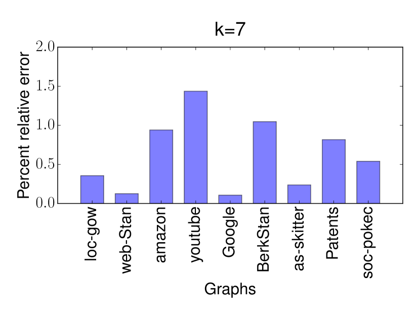
i Percent relative error for k=7

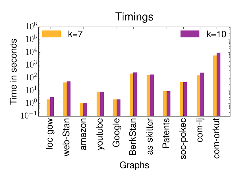
ii Timings for k=7 and k=10

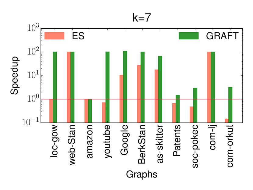
iii Speedup for k=7

Figure 1: Summary of behavior of Turán-shadow over several datasets. Fig. 1i shows the percent relative error in the estimates for k=7 given by Turán-shadow. We only show results for graphs for which we were able to obtain exact counts using either brute force enumeration, or from the results of [18]. The errors are always $<2\%$ and mostly $<1\%$. Fig. 1ii shows the time taken by Turán-shadow for k=7 and k=10. Fig. 1iii shows the speedup (time of algorithm/time of Turán-shadow) over other state of the art algorithms for k=7. The red line indicates a speedup of 1. We could not give a figure for speedup for k=10 because for most instances no competing algorithm terminated in min(7 hours, 100 times Turán-shadow time).

1 Introduction

Pattern counting is an important graph analysis tool in many domains: anomaly detection, social network analysis, bioinformatics among others [21, 27, 10, 29, 22, 17]. Many real world graphs show significantly higher counts of certain patterns than one would expect in a random graph [21, 46, 27]. This technique has been referred to with a variety of names: subgraph analysis, motif counting, graphlet analysis, etc. But the fundamental task is to count the occurrence of a small pattern graph in a large input graph. In all such applications, it is essential to have fast algorithms for pattern counting.

It is well-known that certain patterns capture specific semantic relationships, and thus the social dynamics are reflected in these graph structures. The most famous such pattern is the triangle, which consists of three vertices connected to each other. Triangle counting has a rich history in the social sciences and network science [21, 46, 10, 47].

We focus on the more general problem of clique counting. A $k$-clique is a set of $k$ vertices that are all connected to each other; thus, a triangle is a $3$-clique. Cliques are extremely significant in social network analysis (Chap. 11 of [20] and Chap. 2 of [23]). They are the archetypal example of a dense subgraph, and a number of recent results use cliques to find large, dense subregions of a network [32, 41, 28, 43].

1.1 Problem Statement

Given an undirected graph $G=(V,E)$, a $k$-clique is a set $S$ of $k$ vertices in $V$ with all pairs in $S$ connected by an edge. The problem is to count the number of $k$-cliques, for varying values of $k$. Our aim is to get all clique counts for $k\leq 10$.

The primary challenge is combinatorial explosion. An autonomous system network with ten million edges has more than a trillion $10$-cliques. Any enumeration procedure is doomed to failure. Under complexity theoretical assumptions, clique counting is believed to be exponential in the size $k$ [11], and we cannot hope to get a good worst-case algorithm. Our aim is to employ randomized sampling methods for clique counting, which have seen some success in counting triangles and small patterns [42, 35, 25]. We stress that we make no distributional assumption on the graph. All probabilities are over the internal randomness of the algorithm itself (which is independent of the instance).

1.2 Main contributions

Our main theoretical result is a randomized algorithm Turán-shadow that approximates the $k$-clique count, for any constant $k$. We implement this algorithm on a commodity machine and get $k$-clique counts (for all $k\leq 10$) on a variety of data sets, the largest of which has 100M edges. The main features of our work follow.

• Our novelty is in the algorithmic use of classic extremal combinatorics results on clique densities. Seminal results of Turán [44] and Erdős [16] provide bounds on the number of cliques in a sufficiently dense graph. Turán-shadow tries to cover $G$ by a carefully chosen collection of dense subgraphs that contains all cliques, called a Turán-shadow. It then uses standard techniques to design an unbiased estimator for the clique count. Crucially, the result of Erdős [16] (a quantitative version of Turán’s theorem) is used to bound the variance of the estimator.

  We provide a detailed theoretical analysis of Turán-shadow, proving correctness and analyzing its time complexity. The running time of our algorithm is bounded by the time to construct the Turán-shadow, which as we shall see, is quite feasible in all the experiments we run.

• In the worst case, we cannot expect the Turán-shadow to be small, as that would imply new theoretical bounds for clique counting. But in practice on a wide variety of real graphs, we observe it to be much smaller than the worst-case bound. Thus, Turán-shadow can be made into a practical algorithm, which also has provable bounds. We implement Turán-shadow and run it on a commodity machine. Fig. 1ii shows the time required for Turán-shadow to obtain estimates for $k=7$ and $k=10$ in seconds. The as-skitter graph is processed in less than 3 minutes, despite there being billions of $7$-cliques and trillions of $10$-cliques. All graphs are processed in minutes, except for an Orkut social network with more than 100M edges (Turán-shadow handles this graph within 2.5 hours). To the best of our knowledge, there is no existing work that gets comparable results. An algorithm of Finocchi et al. also computes clique counts, but employs MapReduce on the same datasets [18]. We only require a single machine to get a good approximation.

  We tested Turán-shadow against a number of state of the art algorithmic techniques (color coding [4], edge sampling [42], GRAFT [30]). For 10-clique counting, none of these algorithms terminate for all instances even in 7 hours; Turán-shadow runs in minutes on all but one instance (where it takes less than 2.5 hours). For 7-clique counting, Turán-shadow is typically 10-100 times faster than competing algorithms. (A notable exception is com-orkut, where an edge sampling algorithm runs much faster than Turán-shadow.)

• Turán-shadow has extremely small variance, and computes accurate results (in all instances we could verify). We compute exact results for $7$-clique numbers, and compare with the output of Turán-shadow. In Fig. 1i, we see that the accuracy is well within 2% (relative error) of the true answer for all datasets. We do detailed experiments to measure variance, and in all cases, Turán-shadow is accurate.

  The efficiency and accuracy of Turán-shadow allows us to get clique counts for a variety of graphs, and track how the counts change as $k$ increases. We seem to get two categories of graphs: those where the count increases (exponentially) with $k$, and those where it decreases with $k$, see Fig. 5. This provides a new lens to view social networks, and we hope Turán-shadow can become a new tool for pattern analysis.

1.3 Related Work

The importance of pattern counts gained attention in bioinformatics with a seminal paper of Milo et al. [27], though it has been studied for many decades in the social sciences [21]. Triangle counting and its use has an incredibly rich history, and is used in applications as diverse as spam detection [6], graph modeling [34], and role detection [10]. Counting four cliques is mostly feasible using some recent developments in sampling and exact algorithms [25, 2].

Clique counts are an important part of recent dense subgraph discovery algorithms [32, 41]. Cliques also play an important role in understanding dynamics of social capital [24], and their importance in the social sciences is well documented [20, 23]. In topological approaches to network analysis, cliques are the fundamental building blocks used to construct simplicial structures [36].

From an algorithmic perspective, clique counting has received much attention from the theoretical computer science community [12, 4, 11, 45]. Maximal clique enumeration has been an important topic [3, 37, 15] since the seminal algorithm of Bron-Kerbosch [9]. Practical algorithms for finding the maximum clique were given by Rossi et al. using branch and bound methods [31].

Most relevant to our work is a classic algorithm of Chiba and Nishizeki [12]. This work introduces graph orientations to reduce the search time and provides a theoretical connection to graph arboricity. We also apply this technique in Turán-shadow.

The closest result to our work is a recent MapReduce algorithm of Finocchi et al. for clique counting [18]. This result applies the orientation technique of [12], and creates a large set of small (directed) egonets. Clique counting overall reduces to clique counting in each of these egonets, and this can be parallelized using MapReduce. We experiment on the same graphs used in [18] (particularly, some of the largest ones) and get accurate results on a single, commodity machine (as opposed to using a cluster). Alternate MapReduce methods using multi-way joins have been proposed, though this is theoretical and not tested on real data [1].

A number of randomized techniques have been proposed for pattern counting, and can be used to design algorithms for clique counting. Most prominent are color coding [4, 22, 7, 48] and edge sampling methods [42, 40, 30]. (MCMC methods [8] typically do not scale for graphs with millions of vertices [25].) We perform detailed comparisons with these methods, and conclude that they do not scale for larger clique counting.

2 Main Ideas

The starting point for our result is a seminal theorem of Turán [44]: if the edge density of a graph is more than $1-\frac{1}{k-1}$, then it must contain a $k$-clique. (The density bound is often called the Turán density for $k$.) Erdős proved a stronger version [16]. Suppose the graph has $n$ vertices. Then in this case, it contains $\Omega(n^{k-2})$ $k$-cliques!

Consider the trivial randomized algorithm to estimate $k$-cliques. Simply sample a uniform random set of $k$ vertices and check if they form a clique. Denote the number of $k$-cliques by $C$, then the success probability is $C/{n\choose k}$. Thus, we can estimate this probability using ${n\choose k}/C$ samples. By Erdős’ bound, $C=\Omega(n^{k-2})$. Thus, if the density of a graph (with $n$ vertices) is above the Turán density, one can estimate the number of $k$-cliques using $O(n^{2})$ samples.

Of course, the input graph $G$ is unlikely to have such a high density, and $O(n^{2})$ is a large bound. We try to cover all $k$-cliques in $G$ using a collection of dense subgraphs. This collection is called a Turán shadow. We employ orientation techniques from Chiba-Nishizeki to recursively construct a shadow [12].

We take the degeneracy (k-core) ordering in $G$ [33]. It is well-known that outdegrees are typically small in this ordering. To count $k$-cliques in $G$, it suffices to count $(k-1)$-cliques in every outneighborhood. (This is the main idea in the MapReduce algorithms of Finocchi et al [18].) If an outneighborhood has density higher than the Turán density for $(k-1)$, we add this set/induced subgraph to the Turán shadow. If not, we recursively employ this scheme to find denser sets.

When the process terminates, we have a collection of sets (or induced subgraphs) such that each has density above the Turán threshold (for some appropriate $k^{\prime}$ for each set). Furthermore, the sum of cliques ($k^{\prime}$-cliques, for the same $k^{\prime}$) is the number of $k$-cliques in $G$. Now, we can hope to use the randomized procedure to estimate the number of $k^{\prime}$-cliques in each set of the Turán shadow. By a theorem of Chiba-Nishizeki [12], we can argue that number of vertices in any set of the Turán shadow is at most $\sqrt{2m}$ (where $m$ is the number of edges in $G$). Thus, $O(m)$ samples suffices to estimate clique counts for any set in the Turán shadow.

But the Turán shadow has many sets, and it is infeasible to spend $O(m)$ samples for each set. We employ a randomized trick. We only need to approximate the sum of clique counts over the shadow, and can use random sampling for that purpose. Working through the math, we effectively set up a distribution over the sets in the Turán shadow. We pick a set from this distribution, pick some subset of random vertices, and check if they form a clique. The probability of this event can be related to the number of $k$-cliques in $G$. Furthermore, we can prove that $O(m)$ samples suffice to estimate this probability. All in all, after constructing the Turán shadow, $k$-clique counting can be done in $O(m)$ time.

2.1 Main theorem and significance

The formal version of the main theorem is Theorem 5.8. It requires a fair bit of terminology to state. So we state an informal version that maintains the spirit of our main result. This should provide the reader with a sense of what we can hope to prove. We will define the Turán shadow formally in later sections. But it basically refers to the construct described above.

Theorem 2.1

[Informal] Consider graph $G=(V,E)$ with $n$ vertices, $m$ edges, and maximum core number $\alpha$. Let $\boldsymbol{S}$ be the Turán $k$-clique shadow of $G$, and let $|\boldsymbol{S}|$ be the number of sets in $\boldsymbol{S}$.

Given any $\delta>0,\varepsilon>0,k$, with probability at least $1-\delta$, the procedure Turán-shadow outputs a $(1+\varepsilon)$-multiplicative approximation to the number of $k$-cliques in $G$. The running time is linear in $|\boldsymbol{S}|$ and $m\alpha\log(1/\delta)/\varepsilon^{2}$. The storage is linear in $|\boldsymbol{S}|$.

Observe that the size of the shadow is critical to the procedure’s efficiency. As long as the number of sets in the Turán shadow is small, the extra running time overhead is only linear in $m$. And in practice, we observe that the Turán shadow scales linearly with graph size, leading to a practically viable algorithm.

Outline: In §3, we formally describe Turán’s theorem and set some terminology. §4 defines (saturated) shadows, and shows how to construct efficient sampling algorithms for clique counting from shadow. §5 describes the recursive construction of the Turán shadow. In §5.1, we describe the final procedure Turán-shadow, and prove (the formal version of) Theorem 2.1. Finally, in §6, we detail our empirical study of Turán-shadow and comparison with the state of the art.

3 Turán’s Theorem

For any arbitrary graph $H=(V(H),E(H))$, let $C_{i}(H)$ denote the set of cliques in $H$, and $\rho_{i}(H):=|C_{i}(H)|/{|V(H)|\choose i}$ is the $i$-clique density. Note that $\rho_{2}(H)$ is the standard notion of edge density.

The following theorem of Turán is one of the most important results in extremal graph theory.

Theorem 3.1

(Turán [44]) For any graph $H$, if $\rho_{2}(H)>1-\frac{1}{k-1}$, then $H$ contains a $k$-clique.

This is tight, as evidenced by the complete $(k-1)$-partite graph $T_{n,k-1}$ (also called the Turán graph). In a remarkable generalization, Erdős proved that if an $n$-vertex graph has even one more edge than $T_{n,k-1}$, it must contain many $k$-cliques. One can think of this theorem as a quantified version of Turán’s theorem.

Theorem 3.2

(Erdős [16]) For any graph $H$ over $n$ vertices, if $\rho_{2}(H)>1-\frac{1}{k-1}$, then $H$ contains at least $(n/(k-1))^{k-2}$ $k$-cliques.

It will be convenient to express this result in terms on $k$-clique densities. We introduce some notation: let $f(k)=k^{k-2}/k!$. By Stirling’s approximation, $f(k)$ is well approximated by $e^{k}/\sqrt{2\pi k^{5}}$. Note that $f(k)$ is some fixed constant, for constant $k$. This corollary will be critical to our analysis.

Corollary 3.3

For any graph $H$ over $n$ vertices, if $\rho_{2}(H)>1-\frac{1}{k-1}$, then $\rho_{k}(H)\geq 1/f(k)n^{2}$.

Proof 3.4.

By Theorem 3.2, $H$ has at least $(\frac{n}{(k-1)})^{k-2}$ $k$-cliques. Thus,

$$\rho_{k}(H)\geq\frac{(\frac{n}{(k-1)})^{k-2}}{{n\choose k}}\geq n^{k-2}/n^{k}\times k!/(k-1)^{k-2}\geq 1/(f(k)n^{2})$$

4 Clique shadows

A key concept in our algorithm is that of clique shadows. Consider graph $G=(V,E)$. For any set $S\subseteq V$, we let $C_{\ell}(S)$ denote the set of $\ell$-cliques contained in $S$.

Definition 4.1.

A $k$-clique shadow $\boldsymbol{S}$ for graph $G$ is a multiset of tuples $\{(S_{i},\ell_{i})\}$ where $S_{i}\subseteq V$ and $\ell_{i}\in\mathbb{N}$ such that: there is a bijection between $C_{k}(G)$ and $\bigcup_{(S,\ell)\in\boldsymbol{S}}C_{\ell}(S)$.

Furthermore, a $k$-clique shadow $\boldsymbol{S}$ is $\gamma$-saturated if $\forall(S,\ell)\in\boldsymbol{S}$, $\rho_{\ell}(S)\geq\gamma$.

Intuitively, it is a collection of subgraphs, such that the sum of clique counts within them is the total clique count of $G$. Note that for each set $S$ in the shadow, the associated clique size $\ell$ is different (for different $S$). Observe that $\{(V,k)\}$ is trivally a clique shadow. But it is highly unlikely to be saturated.

It is important to define the size of $\boldsymbol{S}$, which is really the storage required to represent it.

Definition 4.2.

The representation size of $\boldsymbol{S}$ is denoted $\mathrm{size}(\boldsymbol{S})$, and is $\sum_{(S,\ell)\in\boldsymbol{S}}|S|$.

1For each $(S,\ell)\in\boldsymbol{S}$, set $w(S)={|S|\choose\ell}$ ;

2 Set probability distribution $\mathcal{D}$ over $\boldsymbol{S}$ where $p(S)=w(S)/\sum_{(S,\ell)\in\boldsymbol{S}}w(S)$ ;

3 For $r\in 1,2,\ldots,t=\frac{20}{\gamma\varepsilon^{2}}\log(1/\delta)$;

4     Independently sample $(S,\ell)$ from $\mathcal{D}$;

5     Choose a u.a.r. $\ell$-tuple $A$ from $S$;

6      If $A$ forms $\ell$-clique, set indicator $X_{r}=1$. Else, $X_{r}=0$ ;

7 Output $\frac{\sum_{r}X_{r}}{t}\sum_{(S,\ell)\in\boldsymbol{S}}{|S|\choose\ell}$ as estimate for $|C_{k}(G)|$;

Algorithm 1 sample$(\boldsymbol{S},\gamma,k,\varepsilon,\delta)$
$\boldsymbol{S}$ is $\gamma$-saturated $k$-clique shadow
$\varepsilon,\delta$ are error parameters

When a $k$-clique shadow $\boldsymbol{S}$ is $\gamma$-saturated, each $(S,\ell)\in\boldsymbol{S}$ has many $\ell$-cliques. Thus, one can employ random sampling within each $S$ to estimate $|C_{\ell}(S)|$, and thereby estimate $C_{k}(G)$. We use a sampling trick to show that we do not need to estimate all $|C_{\ell}(S)|$; instead we only need $O(1/\gamma)$ samples in total.

Theorem 4.3.

Suppose $\boldsymbol{S}$ is a $\gamma$-saturated $k$-clique shadow for $G$. The procedure sample$(\boldsymbol{S})$ outputs an estimate $\hat{C}$ such $|\hat{C}-|C_{k}(G)||\leq\varepsilon|C_{k}(G)|$ with probability $>1-\delta$.

The running time of sample$(\boldsymbol{S})$ is $O(\mathrm{size}(\boldsymbol{S})+\frac{1}{\gamma\varepsilon^{2}}\log(1/\delta))$.

Proof 4.4.

We remind the reader that $w(S)={|S|\choose\ell}$. Set $\alpha=|C_{k}(G)|/\sum_{S\in\boldsymbol{S}}w(S)$. Observe that

$$\Pr[X_{r}=1] = \sum_{(S,\ell)\in\boldsymbol{S}}\Pr[\textrm{$(S,\ell)$ is chosen}]$$

$$\times \Pr[\textrm{$\ell$-clique chosen in $S$}|\textrm{$(S,\ell)$ is chosen}]$$

The former probability is exactly $w(S)/\sum_{S\in\boldsymbol{S}}w(S)$, and the latter is exactly $|C_{\ell}(S)|/{|S|\choose\ell}$ $=|C_{\ell}(S)|/w(S)$. So,

$$\Pr[X_{r}=1]=\sum_{(S,\ell)\in\boldsymbol{S}}|C_{\ell}(S)|/\sum_{S\in\boldsymbol{S}}w(S)$$

Since $\boldsymbol{S}$ is a $k$-clique shadow, $\sum_{(S,\ell)\in\boldsymbol{S}}|C_{\ell}(S)|=|C_{k}(G)|$. Thus, $\Pr[X_{r}=1]=\alpha$. By the saturation property, $\rho_{\ell}(S)\geq\gamma$, equivalent to $|C_{\ell}(S)|\geq\gamma w(S)$. So $\sum_{S\in\boldsymbol{S}}|C_{\ell}(S)|\geq\gamma\sum_{S\in\boldsymbol{S}}w(S)$. That implies that $\alpha\geq\gamma$. By linearity of expectation, $\hbox{\bf E}[\sum_{r\leq t}X_{r}]=\sum_{r\leq t}\hbox{\bf E}[X_{r}]\geq\gamma t$.

Note that all the $X_{r}$s come from independent trials. (The graph structure plays no role, since the distribution of each $X_{r}$ does not change upon conditioning on the other $X_{r}$s.) By a multiplicative Chernoff bound (Thm 1.1 of [13]),

$$\Pr[\sum_{r}X_{r}/t\leq\alpha(1-\varepsilon)]\leq\exp(-\varepsilon^{2}\hbox{\bf E}[\sum_{r}X_{r}]/3)$$

$$\leq \exp(-\varepsilon^{2}\gamma t/3)=\exp(-5\log(1/\delta))\leq\delta/5.$$

By an analogous upper tail bound, $\Pr[\sum_{r}X_{r}/t\geq\alpha(1+\varepsilon)]\leq\delta/5$. By the union bound, with probability at least $1-2\delta/5$, $\alpha(1-\varepsilon)\leq\sum_{r}X_{r}/t\leq\alpha(1+\varepsilon)$. Note that the output $\hat{C}=(\sum_{r}X_{r}/t)\sum_{S\in\boldsymbol{S}}w(S)$. We multiply the bound above on $\sum_{r}X_{r}/t$ by $\sum_{S\in\boldsymbol{S}}w(S)$, and note that $\alpha\sum_{S\in\boldsymbol{S}}w(S)=|C_{k}(G)|$ to complete the proof.

We stress the significance of Theorem 4.3. Once we get a $\gamma$-saturated clique shadow $\boldsymbol{S}$, $|C_{k}(G)|$ can be approximated in time linear in $\mathrm{size}(\boldsymbol{S})$. The number of samples chosen only depends on $\gamma$ and the approximation parameters, not on the graph size.

But how to actually generate a saturated clique shadow? Saturation appears to be extremely difficult to enforce. This is where the theorem of Erdős (Theorem 3.2) saves the day. It merely suffices to make the edge density of each set in the clique shadow high enough. The $k$-clique density automatically becomes large enough.

Theorem 4.5.

Consider a $k$-clique shadow $\boldsymbol{S}$ such that $\forall(S,\ell)\in\boldsymbol{S}$, $\rho_{2}(S)>1-\frac{1}{\ell-1}$. Let $\gamma=1/\max_{(S,\ell)\in\boldsymbol{S}}f(\ell)|S|^{2}$. Then, $\boldsymbol{S}$ is $\gamma$-saturated.

Proof 4.6.

By Corollary 3.3, for every $(S,\ell)\in\boldsymbol{S}$, $\rho_{\ell}(S)\geq 1/(f(\ell)|S|^{2})$. We simply set $\gamma$ to be the minimum such density over all $(S,\ell)\in\boldsymbol{S}$.

5 Constructing saturated clique shadows

We use a refinement process to construct saturated clique shadows. We start with the trivial shadow $\boldsymbol{S}=\{(V,k)\}$ and iteratively “refine" it until the saturation property is satisfied. By Theorem 4.5, we just have to ensure edge densities in each set are sufficiently large.

For any set $S\subset V$, let $G|_{S}$ be the subgraph of $G$ induced by $S$. Given an unsaturated $k$-clique shadow $\boldsymbol{S}$, we find some $(S,\ell)\in\boldsymbol{S}$ such that $\rho_{2}(S)\leq 1-\frac{1}{\ell-1}$. By iterating over the vertices, we replace $(S,\ell)$ by various neighborhoods in $G|_{S}$ to get a new shadow. We would like the edge densities of these neighborhoods to increase, in the hope of crossing the threshold given in Theorem 4.5.

The key insight is to use the degeneracy ordering to construct specific neighborhoods of high density that also yield a valid shadow. This is basically the classic graph theoretic technique of computing core decompositions, which is widely used in large-graph analysis [33, 19]. As mentioned earlier, this idea is used for fast clique counting as well [12, 18].

Definition 5.1.

For a (labeled) graph $G=(V,E)$, a degeneracy ordering is a permutation of $V$ given as $v_{1},v_{2},\ldots,v_{n}$ such that: for each $i\leq n$, $v_{i}$ is the minimum degree vertex in the subgraph induced by $v_{i},v_{i+1},\ldots,v_{n}$. (As defined, this ordering is not unique, but we can enforce uniqueness by breaking ties by vertex id.)

The degree of $v_{i}$ in $G|_{\{v_{i},\ldots,v_{n}\}}$ is the core number of $v_{i}$. The largest core number is called the degeneracy of $G$, denoted $\alpha(G)$.

The degeneracy DAG of $G$, denoted $D(G)$ is obtained by orienting edges in degeneracy order. In other words, every edge $(u,v)\in G$ is directed from lower to higher in the degeneracy ordering.

The degeneracy ordering is the deletion time of the standard linear time procedure that computes the degeneracy  [26]. It is convenient for us to think of the degeneracy in terms of graph orientations. As defined earlier, any permutation on $V$ can be used to make a DAG out of $G$. We use this idea for generating saturated clique shadows. Essentially, while $G$ may be sparse, out-neighborhoods in $G$ are typically dense. (This has been observed in numerous results on dense subgraph discovery [5, 38, 32].)

We now define the procedure Shadow-Finder$(G,k)$, which works by a simple, iterative refinement procedure. Think of $\boldsymbol{T}$ as the current working set, and $\boldsymbol{S}$ as the final output. We take a set $(S,\ell)$ in $\boldsymbol{T}$, and construct all outneighborhoods in the degeneracy DAG. Any such set whose density is above the Turán threshold goes to $\boldsymbol{S}$ (the output), otherwise, it goes to $\boldsymbol{T}$ (back to the working set).

1Initialize $\boldsymbol{T}=\{(V,k)\}$ and $\boldsymbol{S}=\emptyset$;

2 While $\exists(S,\ell)\in\boldsymbol{T}$ such that $\rho_{2}(S)\leq 1-\frac{1}{\ell-1}$;

3     Construct the degeneracy DAG $D(G|_{S})$;

4     Let $N^{+}_{s}$ denote the outneighborhood (within $D(G|_{S})$) of $s\in S$;

5     Delete $(S,\ell)$ from $\boldsymbol{T}$;

6     For each $s\in S$;

7        If $\ell\leq 2$ or $\rho_{2}(N^{+}_{s})>1-\frac{1}{\ell-2}$;

8           Add $(N^{+}_{s},\ell-1)$ to $\boldsymbol{S}$;

9         Else, add $(N^{+}_{s},\ell-1)$ to $\boldsymbol{T}$;

10 Output $\boldsymbol{S}$;

Algorithm 2 Shadow-Finder$(G,k)$

It is useful to define the recursion tree ${\cal T}$ of this process as follows. Every pair $(S,\ell)$ that is ever part of $\boldsymbol{T}$ is a node in ${\cal T}$. The children of $(S,\ell)$ are precisely the pairs $(N^{+}_{s},\ell-1)$ added in Step 2. (At the point, $(S,\ell)$ is deleted from $\boldsymbol{T}$, and all the $(N^{+}_{s},\ell-1)$ are added.) Observe that the root of $\boldsymbol{T}$ is $(V,k)$, and the leaves are precisely the final output $\boldsymbol{S}$.

Theorem 5.2.

The output $\boldsymbol{S}$ of Shadow-Finder$(G,k)$ is a $\gamma$-saturated $k$-clique shadow, where $\gamma=1/\max_{(S,\ell)\in\boldsymbol{S}}(f(\ell)|S|^{2})$.

Proof 5.3.

We first prove by induction the following loop invariant for Shadow-Finder: $\boldsymbol{T}\cup\boldsymbol{S}$ is always a $k$-clique shadow. For the base case, note that at the beginning, $\boldsymbol{T}=\{(V,k)\}$ and $\boldsymbol{S}=\emptyset$. For the induction step, assume that $\boldsymbol{T}\cup\boldsymbol{S}$ is a $k$-clique shadow at the beginning of some iteration. The element $(S,\ell)$ is deleted from $\boldsymbol{T}$. Each $(N^{+}_{s},\ell-1)$ is added to $\boldsymbol{S}$ or to $\boldsymbol{T}$.

Thus, it suffices to prove that there is a bijection mapping between $C_{\ell}(S)$ and $\bigcup_{s\in S}C_{\ell-1}(N^{+}_{s})$. (By the induction hypothesis, we can then construct a bijection between $C_{k}(G)$ and the appropriate cliques in $\boldsymbol{T}\cup\boldsymbol{S}$.) Consider an $\ell$-clique $K$ in $S$. Set $s$ to be the minimum vertex according to the degeneracy ordering in $D(G|_{S})$. Observe that the remaining vertices form an $(\ell-1)$-clique in $N^{+}_{s}$, which we map the $K$ to. This is a bijection, because every clique $K$ can be mapped to a (unique) $(\ell-1)$-clique, and furthermore, every $(\ell-1)$-clique in $\bigcup_{s\in S}C_{\ell-1}(N^{+}_{s})$ is in the image of this mapping.

Thus, when Shadow-Finder terminates, $\boldsymbol{T}\cup\boldsymbol{S}$ is a $k$-clique shadow. Since $\boldsymbol{T}$ must be empty, $\boldsymbol{S}$ is a $k$-clique shadow. Furthermore, a pair $(S,\ell)$ is in $\boldsymbol{S}$ iff $\rho_{2}(S)>1-\frac{1}{\ell-1}$. By Theorem 4.5, $\boldsymbol{S}$ is $1/\max_{(S,\ell)\in\boldsymbol{S}}(f(\ell)|S|^{2})$-saturated.

We have a simple, but important claim that bounds the size of any set in the shadow by the degeneracy.

Claim 1.

Consider non-root $(S,\ell)\in{\cal T}$. Then $|S|\leq\alpha(G)$.

Proof 5.4.

Suppose the parent of $(S,\ell)$ is $(P,\ell+1)$. Observe that $S$ is the outneighborhood of some node $p$ in the DAG $D(G|_{P})$. Thus, $|S|\leq\alpha(G|_{P})$. The degeneracy can never be larger in a subgraph. (This is apparent by an alternate definition of degeneracy, the maximum smallest degree of an induced subgraph [26].) Hence, $\alpha(G|_{P})\leq\alpha(G)$.

Theorem 5.5.

The running time of Shadow-Finder$(G,k)$ is $O(\alpha(G)\mathrm{size}(\boldsymbol{S})+m+n)$. The total storage is $O(\mathrm{size}(\boldsymbol{S})+m+n)$.

Proof 5.6.

Every time we add $(N^{+}_{S},\ell-1)$ (Step 2) to $\boldsymbol{T}$, we explicitly construct the graph $G|_{N^{+}_{s}}$. Thus, we can guarantee that for every $(S,\ell)$ present in $\boldsymbol{T}$, we can make queries in the graph $G|_{S}$. This construction takes $O(|S|^{2})$ time, to query every pair in $S$. (This is not required when $S=V$, since $G|_{V}=G$.) Furthermore, this construction is done for every $(S,\ell)\in{\cal T}$, except for the root node in ${\cal T}$. Once we have $G|_{S}$, the degeneracy order can be computed in time linear in the number of edges in $G|_{S}$  [26].

Thus, the running time can be bounded by $O(\sum_{(S,\ell)\in{\cal T}:S\neq V}|S|^{2}+m+n)$. By Claim 1, we can bound $\sum_{(S,\ell)\in{\cal T}:S\neq V}|S|^{2}=O(\alpha(G)\sum_{(S,\ell)\in{\cal T}}|S|)$. We split the sum over leaves and non-leaves. The sum over leaves is precisely a sum over the sets in $\boldsymbol{S}$, so that yields $O(\alpha(G)\mathrm{size}(\boldsymbol{S}))$. It suffices to prove that $\sum_{(S,\ell)\in{\cal T}:S\ \textrm{non-leaf}}|S|=O(\mathrm{size}(\boldsymbol{S}))$, which we show next.

Observe that a non-leaf node $(S,\ell)$ in ${\cal T}$ has exactly $|S|$ children, one for each vertex $s\in S$. Thus,

$$\sum_{(S,\ell)\in{\cal T}:(S,\ell)\textrm{non-leaf}}|S| = \sum_{(S,\ell)\in{\cal T}}\textrm{\# children of $(S,\ell)$}$$

$$= {\cal T}$$ # edges in

All internal nodes in ${\cal T}$ have at least $2$ children, so the number of edges in ${\cal T}$ is at most twice the number of leaves in ${\cal T}$. But this is exactly the number of sets in the output $\mathcal{S}$, which is at most $\mathrm{size}(\boldsymbol{S})$.

The total storage is $O(\sum_{(S,\ell)\in{\cal T}}|S|+m+n)$, which is $O(\mathrm{size}(S)+m+n)$ by the above arguments.

We now formally define the Turán shadow to be output of this procedure.

Definition 5.7.

The $k$-clique Turán shadow of $G$ is the output of Shadow-Finder$(G,k)$.

5.1 Putting it all together

1Compute $\boldsymbol{S}=$ Shadow-Finder$(G,k)$;

2 Set $\gamma=1/\max_{(S,\ell)\in\boldsymbol{S}}(f(\ell)|S|^{2})$;

3 Output $\hat{C}_{k}={\tt sample}(G,k,\gamma,\varepsilon,\delta)$;

Algorithm 3 Turán-shadow$(G,k,\varepsilon,\delta)$

Theorem 5.8.

Consider graph $G=(V,E)$ with $m$ edges, $n$ vertices, and degeneracy $\alpha(G)$. Assume $m\leq n^{2}/4$. Let $\boldsymbol{S}$ be the Turán $k$-clique shadow of $G$.

With probability at least $1-\delta$ (this probability is over the randomness of Turán-shadow; there is no stochastic assumption on $G$), $|\hat{C}_{k}-|C_{k}(G)||\leq\varepsilon|C_{k}(G)|$.

The running time of Turán-shadow is $O(\alpha(G)\mathrm{size}(\boldsymbol{S})+f(k)m\log(1/\delta)/\varepsilon^{2}+n)$ and the total storage is $O(\mathrm{size}(\boldsymbol{S})+m+n)$.

Proof 5.9.

By Theorem 5.2, $\boldsymbol{S}$ is $\gamma$-saturated, for $\gamma=1/\max_{(S,\ell)\in\boldsymbol{S}}f(\ell)|S|^{2}$. Since $m\leq n^{2}/4$, the procedure Shadow-Finder$(G,k)$ cannot just output $\{(V,k)\}$. All leaves in the recursion tree must have depth at least $2$, and by Claim 1, for all $(S,\ell)\in\boldsymbol{S}$, $|S|\leq\alpha(G)$. A classic bound on the degeneracy asserts that $\alpha(G)\leq\sqrt{2m}$ (Lemma 1 of [12]). Since $f(\ell)$ is increasing in $\ell$, $\max_{(S,\ell)\in\boldsymbol{S}}f(\ell)|S|^{2}\leq 2f(k)m$. Thus, $\gamma=\Omega(1/(f(k)m))$.

By Theorem 4.3, the running time of sample is $O(\mathrm{size}(\boldsymbol{S})+\log(1/\delta)/(\gamma\varepsilon^{2}))$, which is $O(\mathrm{size}(\boldsymbol{S})+f(k)m\log(1/\delta)/\varepsilon^{2})$. Theorem 4.3 also asserts the accuracy of the output. Adding the bounds of Theorem 5.5, we prove the running time and storage bounds.

5.2 The shadow size

The practicality of Turán-shadow hinges on $\mathrm{size}(\boldsymbol{S})$ being small. It is not hard to prove a worst-case bound, using the degeneracy.

Claim 2.

$\mathrm{size}(\boldsymbol{S})=O(n\alpha(G)^{k-2})$.

Proof 5.10.

By arguments in the proof of Theorem 5.5, we can show that $\mathrm{size}(\boldsymbol{S})$ is at most the number of edges in ${\cal T}$. In ${\cal T}$, the degree of the root is $n$, and by Claim 1, the degree of all other nodes is at most $\alpha(G)$. The depth of the tree is at most $k-1$, since the value of $\ell$ decreases every step down the tree. That proves that $n\alpha^{k-2}$ bound.

This bound is not that interesting, and the Chiba-Nishizeki algorithm for exact clique enumeration matches this bound [12]. Indeed, we can design instances where Claim 2 is tight (a set of $n/\alpha$ Erdős-Rényi graphs $G_{\alpha,1/3}$). In any case, beating an exponential dependence on $k$ for any algorithm is unlikely [11].

The key empirical insight of this paper is that Turán clique shadows are small for real-world graphs. We explain in more detail in the next section; Fig. 3 shows that the shadow sizes are typically less than $m$, and never more than $10m$.

6 Experimental results

Preliminaries: We implemented our algorithms in C++ and ran our experiments on a commodity machine equipped with a 3.00GHz Intel Core i7 processor with 8 cores and 256KB L2 cache (per core), 20MB L3 cache, and 128GB memory.

We performed our experiments on a collection of graphs from SNAP [49], the largest with more than 100M edges. The collection includes social networks, web networks, and infrastructure networks. Each graph is made simple by ignoring direction. Basic properties of these graphs are presented in Tab. 2.

In the implementation of Turán-shadow, there is just one parameter to choose: the number of samples chosen in Step 1 in sample. Theoretically, it is set to $(20/\gamma\varepsilon^{2})\log(1/\delta)$; in practice, we just set it to 50K for all our runs. Note that $\gamma$ is not a free parameter and is automatically set in Step 3 of Turán-shadow.

We focus on counting $k$-cliques for $k$ ranging from $5$ to $10$. We ignore $k=3,4$, since there is much existing (scalable) work for this setting [35, 25, 2]. For the sake of presentation, we showcase results for $k=7,10$. We focus on $k=10$ since no existing algorithm produces results for 10-cliques in reasonable time. We also show specifics for $k=7$, to contrast with $k=10$.

Table 1: Graph properties

k=5 k=7 k=10 graph vertices edges degen max degree estimate % error time estimate % error time estimate % error time loc-gowalla 1.97E+05 9.50E+05 51 14730 1.46E+07 0.20 2 4.78E+07 0.36 2 1.08E+08 1.63 3 web-Stanford 2.82E+05 1.99E+06 71 38625 6.21E+08 0.00 20 3.47E+10 0.13 43 5.82E+12 - 52 amazon0601 4.03E+05 4.89E+06 10 2752 3.64E+06 0.93 1 9.98E+05 0.95 1 9.77E+03 0.01 1 com-youtube 1.13E+06 2.99E+06 51 28754 7.29E+06 1.08 7 7.85E+06 1.38 8 1.83E+06 0.20 8 web-Google 8.76E+05 4.32E+06 44 6332 1.05E+08 0.10 2 6.06E+08 0.09 2 1.29E+10 0.82 2 web-BerkStan 6.85E+05 6.65E+06 201 84230 2.19E+10 0.00 101 9.30E+12 1.05 214 5.79E+16 - 262 as-skitter 1.70E+06 1.11E+07 111 35455 1.17E+09 0.01 153 7.30E+10 0.23 164 1.42E+13 - 180 cit-Patents 3.77E+06 1.65E+07 64 793 3.05E+06 0.34 10 1.89E+06 0.83 9 2.55E+03 4.46 9 soc-pokec 1.63E+06 2.23E+07 47 14854 5.29E+07 0.13 42 8.43E+07 0.48 45 1.98E+08 0.01 45 com-lj 4.00E+06 3.47E+07 360 14815 2.46E+11 - 106 4.48E+14 - 153 1.47E+19 - 252 com-orkut 3.07E+06 1.17E+08 253 33313 1.57E+10 0.00 3119 3.61E+11 1.97 5587 3.03E+13 - 9298

Table 2: Table shows the sizes, degeneracy, maximum degree of the graphs, the counts of 5, 7 and 10 cliques obtained using Turán-shadow, the percent relative error in the estimates, and time in seconds required to get the estimates. Some of the exact counts were obtained from  [18] (where available). This is the first such algorithm that obtains these counts with $<2\%$ error without using any specialized hardware.

Convergence of Turán-shadow: We picked two smaller graphs amazon0601 and web-Google for which the exact $k$-clique count is known (for all $k\in[5,10]$). We choose both $k=7,10$. For each graph, for sample size in [10K,50K,100K,500K,1M], we perform 100 runs of the algorithm. We plot the spread of the output of Turán-shadow, over all these runs. The results are shown in Fig. 2. The red line denotes the true answer, and there is a point for the output of every single run. Even for 10-clique counting, the spread of 100 runs is absolutely minimal. For 50K samples, the range of values is within 2% of the true answer. This was consistent with all our runs.

Accuracy of Turán-shadow: For many graphs (and values of $k$), it was not feasible to get an exact algorithm to run in reasonable time. The run time of exact procedures can vary wildly, so we have exact numbers for some larger graphs but could not generate numbers for smaller graphs. We collected as many exact results as possible to validate Turán-shadow. For the sake of presentation, we only show a snapshot of these results here.

For $k=7$, we collected exact results for a collection of graphs, and for each graph, compared the output of a single run of Turán-shadow (with 50K samples) with the true answer. We compute relative error: |true - estimate|/true. These results are presented in Fig. 1i. Note that the errors are within 2% in all cases, again consistent with all our runs.

In Tab. 2, we present the output of our algorithm for a single run on all instances and $k=5,7,10$. For every graph where we know the true value, we present the relative error. Barring one example (cit-Patents for $k=10$), all errors are less than 2%. Even in the worst case, the error is at most 5%.

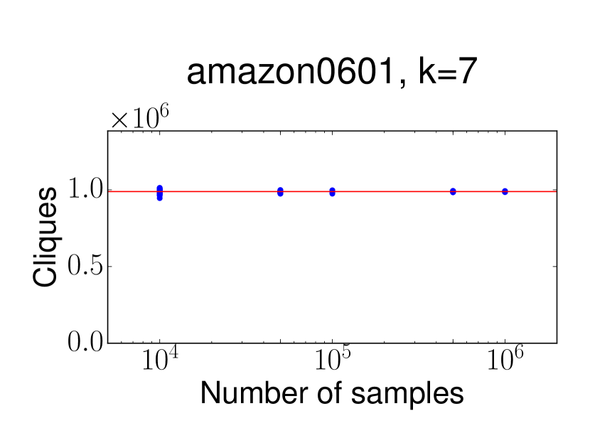
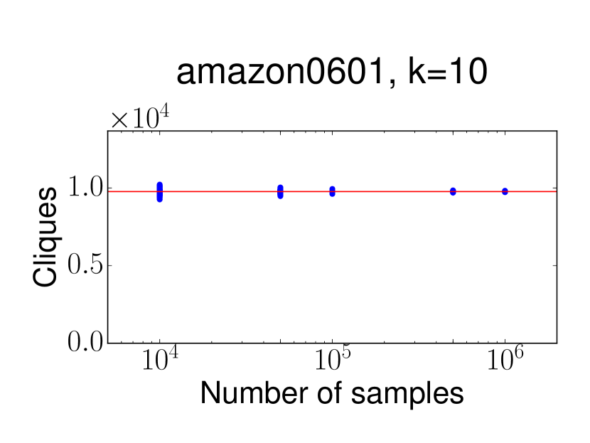
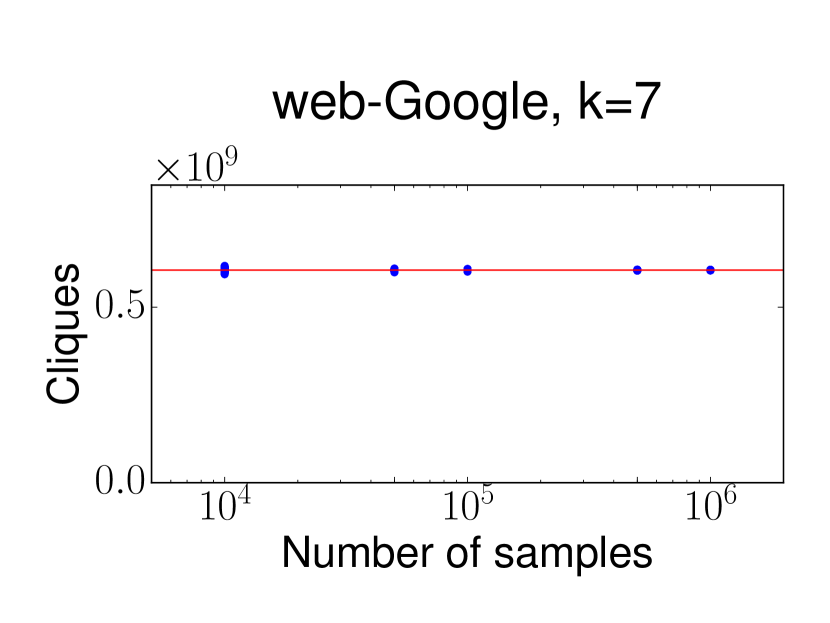
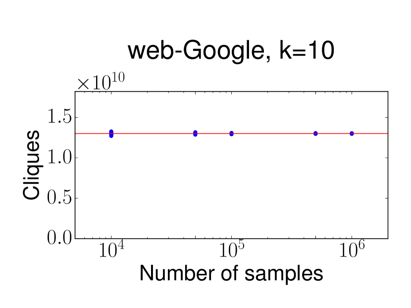
Figure 2: Figure shows convergence over 100 runs of Turán-shadow using 10K, 50K, 100K, 500K and 1M samples each. Turán-shadow has an extremely low spread and consistently gives very accurate results.

Running time: All runtimes are presented in Tab. 2. (We show the time for a single run, since there was little variance for different runs on the same graph.) In all instances except com-orkut, the runtime was a few minutes, even for graphs with tens of millions of edges. We stress that these are all on a single machine. For com-orkut, the runtime is at most 2.5 hours. Previously, such graphs were processed with MapReduce on clusters [18].

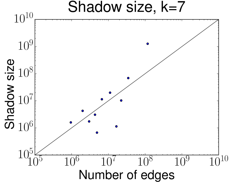
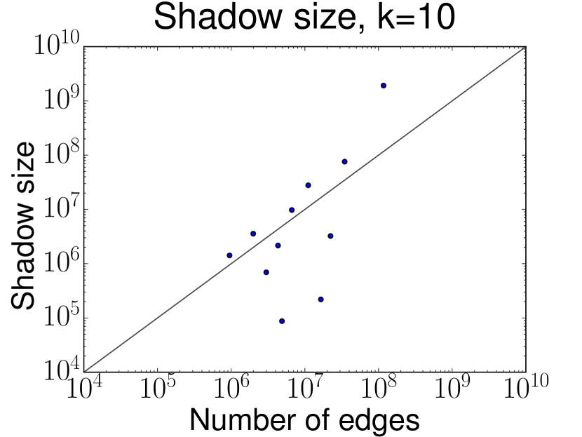
Figure 3: Figures show the sizes of the Turán shadows generated for k=7 and k=10 in all the graphs. The runtime of the algorithm is proportional to the size of the shadow and crucially, the sizes scale only linearly with the number of edges.

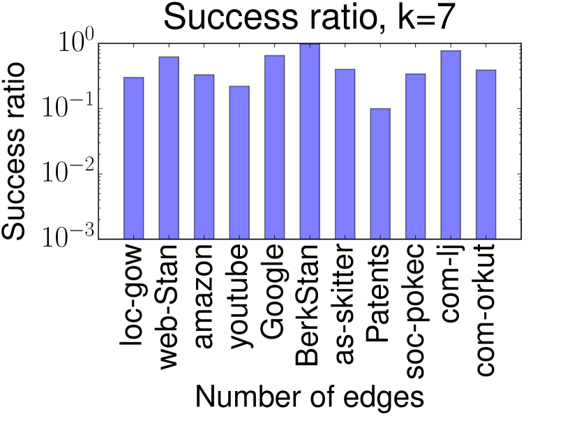
Figure 4: Figures show the success ratio (probability of finding a clique) obtained in the sampling experiments in all the graphs.

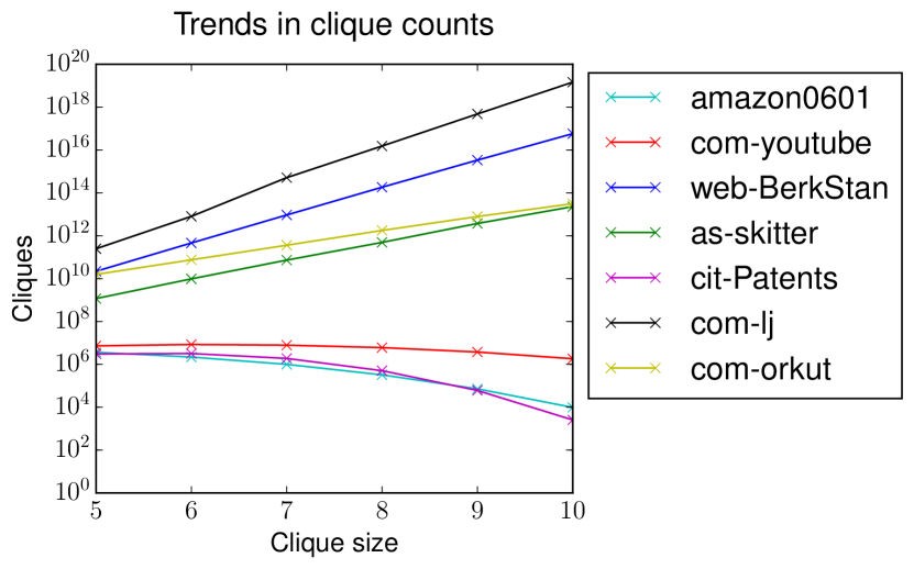
Figure 5: Figures show the trends in clique counts of some graphs. While cit-Patents, com-youtube and amazon0601 show a decreasing trend, all other graphs show an exponential increase in the number of cliques with clique size.

6.1 Comparison with other algorithms

Our exact brute-force procedure is a well-tuned algorithm that uses the degeneracy ordering and exhaustively searches outneighborhoods for cliques. This is basically the procedure of Finetti et al. [18], inspired by the algorithm of Chiba-Nishizeki [12]. We compare with the following algorithms.

• Color coding: This is a classic algorithmic technique [4]. For counting $k$-cliques, the algorithm randomly colors vertices with one of $k$ colors. Then, the algorithm uses a brute-force procedure to count polychromatic $k$-cliques (where each vertex has a different color). This number is scaled to give an unbiased estimate, and the coloring helps cut down the search time of the brute-force procedure. This method has been applied in practice for numerous pattern counting problems [22, 7, 48].

• Edge sampling: Edge sampling was discussed by Tsourakakis et al. in the context of triangle counting [42, 39, 40], though the idea is flexible and can be used for large patterns [14]. The idea here is to sample each edge independently with some probability $p$, and then count $k$-cliques in the down-sampled graph. This number is scaled to give an unbiased estimate for the number of $k$-cliques.

  For clique counting, we observe that minor differences in $p$ (by $0.1$) have huge effects on runtime and accuracy. To do a fair comparison, we run multiple experiments with varying $p$ (increments of $0.1$), until we reach the smallest $p$ that consistently yields less than 5% error. (Note that the error of Turán-shadow is significantly smaller that this.) Timing comparisons are done with runs for that value of $p$.

• GRAFT [30]: Rahman et al. give a variant of edge sampling with better performance for large pattern counts [30]. The idea is to sample some set of edges, and exactly count the number of $k$-cliques on each of these edges. This can be scaled into an unbiased estimate for the total number of $k$-cliques.

  As with edge sampling, we increase the number of edge samples until we get consistently within 5% error. Timing comparisons are done with this setting. Typical settings seems to be in the range of 100K to 1M samples. Beyond that, GRAFT is infeasible, even for graphs with 10M edges.

We focus on $k=7,10$ for clarity. In all cases, we simply terminate the algorithm if it takes more than the minimum of 7 hours and 100 times the time required by Turán-shadow. We present the speedup of Turán-shadow with respect to all these algorithms in Fig. 1iii for k=7. For k=10, for most instances, no competing algorithm terminated.

• $k=7$ (Fig. 1iii): Turán-shadow outperformed Color Coding and GRAFT across all instances. Color Coding never gave good accuracy, so we ignore it in our speedup plots. We do note that Edge Sampling gives extremely good performance in some instances, but can be very slow in others. For amazon0601, com-youtube, cit-Patents, and soc-pokec, Edge Sampling is faster than Turán-shadow. But Turán-shadow handles all these graphs with a minute. The only exception is com-orkut, where GRAFT is much faster than Turán-shadow. We note that all other algorithms can perform extremely poorly on fairly small graphs: Edge Sampling is 10-100 times slower on a number of graphs, which have only millions of edges. On the other hand, Turán-shadow always runs in minutes for these graphs.

• $k=10$ : No competing algorithm is able to handle 10 cliques for all datasets, even in 7 hours (giving a speedup of anywhere between 3x to 100x). They all generally fail for at least half of the instances. Turán-shadow gets an answer for com-orkut within 2.5 hours, and handles all other graphs in minutes.

6.2 Details about Turán-shadow

Shadow size: In Fig. 3, we plot the size of the $k$-clique Turán shadow with respect to the number of edges in each instance. This is done for $k=7,10$. (The line $y=x$ is drawn as well.) As seen from Theorem 5.8, the size of the shadow controls the storage and runtime of Turán-shadow. We see how in almost all instances, the shadow size is around the number of edges. This empirically explains the efficiency of Turán-shadow. The worst case is com-orkut, where the shadow size is at most ten times the number of edges.

Success probability: The final estimate of Turán-shadow is generated through sample. We asserted (theoretically) that $O(m)$ samples suffice, and in practice, we use 50K samples. In Fig. 4, we plot (for $k=7,10$) the empirical probability of finding a clique in Step 1 of sample. The higher this is, the fewer samples we require and the more confidence in the statistical validity of our estimate. Almost all (empirical) probabilities are more than $0.1$, and 50K samples are more than enough for convergence.

Trends in clique numbers: Fig. 5 plots the number of $k$-cliques (as computed by Turán-shadow) versus $k$. (We do not consider all graphs for the sake of clarity.) Interestingly, there are some graphs where the number of cliques grows exponentially. This is probably because of a large clique/dense-subgraph, and it would be interesting to verify this. For another class of graphs, the clique counts are consistently decreasing. This seems to classify graphs into one of two types. We feel further analysis of these trends would be interesting, and Turán-shadow can be a useful tool for network analysis.

References

- [1] F. N. Afrati, D. Fotakis, and J. D. Ullman. Enumerating subgraph instances using map-reduce. In International Conference on Data Engineering (ICDE), pages 62–73, 2013.
- [2] N. K. Ahmed, J. Neville, R. A. Rossi, and N. Duffield. Efficient graphlet counting for large networks. In Proceedings of International Conference on Data Mining (ICDM), 2015.
- [3] E. A. Akkoyunlu. The enumeration of maximal cliques of large graphs. SIAM J. Comput., 2:1–6, 1973.
- [4] N. Alon, R. Yuster, and U. Zwick. Color-coding: A new method for finding simple paths, cycles and other small subgraphs within large graphs. In Symposium on the Theory of Computing (STOC), pages 326–335, 1994.
- [5] R. Andersen and K. Chellapilla. Finding dense subgraphs with size bounds. In Workshop on Algorithms and Models for the Web-Graph (WAW), pages 25–37, 2009.
- [6] L. Becchetti, P. Boldi, C. Castillo, and A. Gionis. Efficient semi-streaming algorithms for local triangle counting in massive graphs. In KDD’08, pages 16–24, 2008.
- [7] N. Betzler, R. van Bevern, M. R. Fellows, C. Komusiewicz, and R. Niedermeier. Parameterized algorithmics for finding connected motifs in biological networks. IEEE/ACM Trans. Comput. Biology Bioinform., 8(5):1296–1308, 2011.
- [8] M. Bhuiyan, M. Rahman, M. Rahman, and M. A. Hasan. Guise: Uniform sampling of graphlets for large graph analysis. In Proceedings of International Conference on Data Mining, pages 91–100, 2012.
- [9] C. Bron and J. Kerbosch. Algorithm 457: Finding all cliques of an undirected graph. Commun. ACM, 16(9):575–577, Sept. 1973.
- [10] R. Burt. Structural holes and good ideas. American Journal of Sociology, 110(2):349–399, 2004.
- [11] J. Chen, X. Huang, I. A. Kanj, and G. Xia. Linear FPT reductions and computational lower bounds. In L. Babai, editor, Symposium on the Theory of Computing (STOC), pages 212–221. ACM, 2004.
- [12] N. Chiba and T. Nishizeki. Arboricity and subgraph listing algorithms. SIAM J. Comput., 14:210–223, 1985.
- [13] D. Dubhashi and A. Panconesi. Concentration of Measure for the Analysis of Randomized Algorithms. Cambridge University Press, 2009.
- [14] E. R. Elenberg, K. Shanmugam, M. Borokhovich, and A. G. Dimakis. Distributed estimation of graph 4-profiles. In J. Bourdeau, J. Hendler, R. Nkambou, I. Horrocks, and B. Y. Zhao, editors, World Wide Web (WWW), pages 483–493. ACM, 2016.
- [15] D. Eppstein and D. Strash. Listing all maximal cliques in large sparse real-world graphs. In P. M. Pardalos and S. Rebennack, editors, Symposium of Experimental Algorithms, volume 6630 of Lecture Notes in Computer Science, pages 364–375. Springer, 2011.
- [16] P. Erdős. On the number of complete subgraphs and circuits contained in graphs. Casopis Pest. Mat., 94:290–296, 1969.
- [17] K. Faust. A puzzle concerning triads in social networks: Graph constraints and the triad census. Social Networks, 32(3):221–233, 2010.
- [18] I. Finocchi, M. Finocchi, and E. G. Fusco. Clique counting in mapreduce: Algorithms and experiments. ACM Journal of Experimental Algorithmics, 20, 2015.
- [19] C. Giatsidis, F. Malliaros, D. M. Thilikos, and M. Vazirgiannis. Corecluster: A degeneracy based graph clustering framework. In IAAA: Innovative Applications of Artificial Intelligence, 2014.
- [20] R. A. Hanneman and M. Riddle. Introduction to social network methods. University of California, Riverside, 2005. http://faculty.ucr.edu/~hanneman/nettext/.
- [21] P. Holland and S. Leinhardt. A method for detecting structure in sociometric data. American Journal of Sociology, 76:492–513, 1970.
- [22] F. Hormozdiari, P. Berenbrink, N. Przulj, and S. C. Sahinalp. Not all scale-free networks are born equal: The role of the seed graph in ppi network evolution. PLoS Computational Biology, 118, 2007.
- [23] M. O. Jackson. Social and Economic Networks. Princeton University Press, 2010.
- [24] M. O. Jackson, T. Rodriguez-Barraquer, and X. Tan. Social capital and social quilts: Network patterns of favor exchange. American Economic Review, 102(5):1857?1897, 2012.
- [25] M. Jha, C. Seshadhri, and A. Pinar. Path sampling: A fast and provable method for estimating 4-vertex subgraph counts. In World Wide Web (WWW), pages 495–505, 2015.
- [26] D. W. Matula and L. L. Beck. Smallest-last ordering and clustering and graph coloring algorithms. Journal of the ACM (JACM), 30(3):417–427, 1983.
- [27] R. Milo, S. Shen-Orr, S. Itzkovitz, N. Kashtan, D. Chklovskii, and U. Alon. Network motifs: Simple building blocks of complex networks. Science, 298(5594):824–827, 2002.
- [28] M. Mitzenmacher, J. Pachocki, R. Peng, C. E. Tsourakakis, and S. C. Xu. Scalable large near-clique detection in large-scale networks via sampling. In SIGKDD International Conference on Knowledge Discovery and Data Mining, pages 815–824, 2015.
- [29] N. Przulj, D. G. Corneil, and I. Jurisica. Modeling interactome: scale-free or geometric?. Bioinformatics, 20(18):3508–3515, 2004.
- [30] M. Rahman, M. A. Bhuiyan, and M. A. Hasan. Graft: An efficient graphlet counting method for large graph analysis. IEEE Transactions on Knowledge and Data Engineering, PP(99), 2014.
- [31] R. A. Rossi, D. F. Gleich, and A. H. Gebremedhin. Parallel maximum clique algorithms with applications to network analysis. SIAM Journal on Scientific Computing, 37(5):C589–C616, 2015.
- [32] A. E. Sariyüce, C. Seshadhri, A. Pinar, and Ü. V. Çatalyürek. Finding the hierarchy of dense subgraphs using nucleus decompositions. pages 927–937, 2015.
- [33] S. B. Seidman. Network structure and minimum degree. Social Networks, 5(3):269–287, 1983.
- [34] C. Seshadhri, T. G. Kolda, and A. Pinar. Community structure and scale-free collections of Erdös-Rényi graphs. Physical Review E, 85(5):056109, May 2012.
- [35] C. Seshadhri, A. Pinar, and T. G. Kolda. Fast triangle counting through wedge sampling. In Proceedings of the SIAM Conference on Data Mining, 2013.
- [36] A. Sizemore, C. Giusti, and D. S. Bassett. Classification of weighted networks through mesoscale homological features. Journal of Complex Networks, 10.1093, 2016.
- [37] E. Tomita, A. Tanaka, and H. Takahashi. The Worst-Case Time Complexity for Generating All Maximal Cliques, pages 161–170. Springer Berlin Heidelberg, Berlin, Heidelberg, 2004.
- [38] C. Tsourakakis, F. Bonchi, A. Gionis, F. Gullo, and M. Tsiarli. Denser than the densest subgraph: Extracting optimal quasi-cliques with quality guarantees. In Knowledge Data and Discovery (KDD), 2013.
- [39] C. Tsourakakis, P. Drineas, E. Michelakis, I. Koutis, and C. Faloutsos. Spectral counting of triangles in power-law networks via element-wise sparsification. In ASONAM’09, pages 66–71, 2009.
- [40] C. Tsourakakis, M. N. Kolountzakis, and G. Miller. Triangle sparsifiers. J. Graph Algorithms and Applications, 15:703–726, 2011.
- [41] C. E. Tsourakakis. The k-clique densest subgraph problem. In Proceedings of the Conference on World Wide Web WWW, pages 1122–1132, 2015.
- [42] C. E. Tsourakakis, U. Kang, G. L. Miller, and C. Faloutsos. Doulion: counting triangles in massive graphs with a coin. In Knowledge Data and Discovery (KDD), pages 837–846, 2009.
- [43] C. E. Tsourakakis, J. W. Pachocki, and M. Mitzenmacher. Scalable motif-aware graph clustering. CoRR, abs/1606.06235, 2016.
- [44] P. Turán. On an extremal problem in graph theory. Mat. Fiz. Lapok, 48(436-452):137, 1941.
- [45] V. Vassilevska. Efficient algorithms for clique problems. Information Processing Letters, 109(4):254 – 257, 2009.
- [46] D. Watts and S. Strogatz. Collective dynamics of ‘small-world’ networks. Nature, 393:440–442, 1998.
- [47] B. Welles, A. Van Devender, and N. Contractor. Is a friend a friend?: Investigating the structure of friendship networks in virtual worlds. In CHI-EA’10, pages 4027–4032, 2010.
- [48] Z. Zhao, G. Wang, A. Butt, M. Khan, V. S. A. Kumar, and M. Marathe. Sahad: Subgraph analysis in massive networks using hadoop. In Proceedings of International Parallel and Distributed Processing Symposium (IPDPS), pages 390–401, 2012.
- [49] Stanford Network Analysis Project (SNAP). Available at http://snap.stanford.edu/.