Bayesian Semiparametric Mixed Effects Markov Chains

Abstract

Studying the neurological, genetic and evolutionary basis of human vocal communication mechanisms using animal vocalization models is an important field of neuroscience. The data sets typically comprise structured sequences of syllables or ‘songs’ produced by animals from different genotypes under different social contexts. We develop a novel Bayesian semiparametric framework for inference in such data sets. Our approach is built on a novel class of mixed effects Markov transition models for the songs that accommodates exogenous influences of genotype and context as well as animal specific heterogeneity. We design efficient Markov chain Monte Carlo algorithms for posterior computation. Crucial advantages of the proposed approach include its ability to provide insights into key scientific queries related to global and local influences of the exogenous predictors on the transition dynamics via automated tests of hypotheses. The methodology is illustrated using simulation experiments and the aforementioned motivating application in neuroscience.

Some Key Words: Bayesian nonparametrics, Categorical sequences, Markov chains, Mixed effects models, Mouse vocalization experiments.

Short Title: Mixed Effects Markov Chains

1 Introduction

This article introduces a novel class of mixed effects Markov models for categorical sequences recorded under the influence of exogenous categorical predictors. The predictors themselves do not vary sequentially but remain fixed for the entire lengths of the sequences. Additionally, each sequence may be associated with an individual selected at random from a larger population of interest and may thus be influenced by random effects specific to the chosen subjects. Our inferential goals include estimation of transition probabilities governing the stochastic evolution of the sequences as well as an assessment of the importance of the predictors in influencing the transition dynamics.

While the literature on Markov models and its various derivatives and extensions is enormous, owing to numerous methodological and computational challenges, the literature on mixed effects Markov models is relatively sparse in spite of their immense potential and general practical utility.

Generalized linear models (GLM) provide one route to modeling mixed effects Markov chains. However, except for binary sequences, specifying flexible predictor-dependent Markov models using traditional GLMs is daunting. Consider, for example, an adaptation of the multinomial logit model (McCullagh and Nelder, 1989; Agresti, 2013) to our setting. With $p$ categorical predictors $x_{j}$ with $d_{j}$ categories each, $j=1,\dots,p$, and response sequences $y_{t}$ comprising $d_{0}$ categories, even without any interaction or random effects, such a specification would require formulating $d_{0}-1$ models, one for each $y_{t}=1,\dots,d_{0}-1$, with $\sum_{j=0}^{p}(d_{j}-1)$ dummy variables representing local dependence and predictors $y_{t-1},x_{1},\dots,x_{p}$ included as linear predictors on the logit scale. Interactions and random effects greatly add to the complexity; for example, due to the lack of analytic forms marginalizing out the random effects. Inferences under such models and testing of hypotheses become intractable. Hence, relevant work in the literature has focused on very simple scenarios, such as binary sequences, single predictors, and models excluding interactions and random effects (Bonney, 1987; Fitzmaurice and Liard, 1993; Azzalini, 1994; Schildcrout and Heagerty, 2005, 2007; Rahman and Islam, 2007; Bizzotto et al., 2010; Islam et al., 2013).

Markov chains provide building blocks for many other important dynamical systems, including hidden Markov models (HMM). HMMs consist of a latent process $y_{t}$, evolving according to a Markov chain, and an observed process $z_{t}$, evolving independently, given $y_{t}$. Hudges and Guttorp (1994) and Spezia (2006) developed fixed effects HMMs with sequentially varying predictors influencing the transition dynamics of the latent sequence. Turner et al. (1998) and Wang and Puterman (1999) discussed mixed effects HMMs for count data, but incorporated the covariate effects only through the observed process. See also Maruotti and Rydén (2009); Delattre (2010); Maruotti (2011) and Rueda et al. (2013). Altman (2007) developed a mixed HMM, adopting a multinomial logit model based approach to incorporate mixed effects in the transition distributions, but focused only on models with binary sequences with a single binary predictor in real and simulated illustrations. Additional discussions on these models are presented in the Supplementary Materials.

This article presents a fundamentally different approach to modeling mixed effects Markov chains directly motivated by mouse vocalization experiments. Our proposed Bayesian hierarchical formulation provides flexible, easily interpretable representations of exogenous predictor dependent individual specific transition probability matrices, borrowing information across sequences via a layered hierarchy. We include fixed and random effects directly on the probability scale, avoiding issues in choosing link functions and facilitating computational simplifications. Using Dirichlet distributed random effects, we obtain analytic forms for the population level probabilities. To reduce dimensionality, the model clusters levels of predictors that have similar impact on the transition dynamics. The model structure leads to a stable and efficient Markov chain Monte Carlo (MCMC) algorithm. Estimates of the posterior probabilities of global and local hypotheses are easily available from samples drawn by the algorithm.

The article is organized as follows. Section 2 describes the neuroscience applications that motivated our research. Section 3 develops the model. Section 4 describes MCMC algorithms to sample from the posterior. Section 5 presents the results of the proposed method applied to mouse vocalization data. Section 6 presents the results of simulation experiments. Section 7 contains concluding remarks.

2 Mouse Vocalization Experiments

While the statistical problem that we address is of broad scope, our research was motivated by studies of the genetic and evolutionary basis of human vocal communication. Spoken language plays a central role in human culture. We belong to one of few species that can learn to produce new vocalizations, which we use to express emotions, convey ideas, and communicate. These vocal behaviors are susceptible to a range of impairments, making dramatic impacts on everyday life and presenting a major public health issue, with the prevalence of speech-sound disorders in young children estimated at 8-9 percent (NIH-NIDCD Report, 2010). Such disorders are highly heritable, but causes are typically unknown (Law et al., 2000).

Many species of birds have the ability to sing complex songs to communicate information within and across species (Marler and Slabbekoorn, 2004). Songbirds are vocal learners like us and their songs are similar in many ways to human languages. Extensive research spanning over the last six decades has shown that songbirds provide an immensely useful model for studying the neuroscience of human vocal communication systems (Zeigler and Marler, 2008). Aside the human aspect, studying birds provides insights into the evolution of vocal communication skills across species (Kaas, 2006).

Holy and Guo (2005) discovered that male mice ‘sing’ ultrasonic vocalizations (USVs) with some features similar to courtship songs of songbirds. Being mammals, mice have a lot more in common with humans in terms of genetic makeup, anatomy and physiology. Mice are also easier to manipulate genetically and less expensive to raise in controlled laboratory environments. In recent years, neuroscientists have thus invested tremendous efforts in studying the mouse vocalization system. Studies have confirmed that male mice emit USV songs in sexual and other contexts using a multisyllabic repertoire. The syllables can be categorized based on spectral features (Holy and Guo, 2005; Scattoni et al., 2008b; Arriaga et al., 2012). Chabout et al. (2012, 2015) grouped syllables into four categories - simple syllables without any pitch jumps (‘s’); complex syllables containing two notes separated by a single upward (‘u’) or downward (‘d’) pitch jump; and more complex syllables containing a series of multiple pitch jumps (‘m’). See Figure 1. Syllable durations and inter-syllable intervals are typically between 0 and 250 ms (Chabout et al., 2015; Castellucci et al., 2016). Each interval of 250ms that a mouse remains silent is thus classified as a special silence syllable (‘x’).

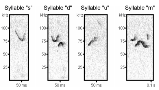
Figure 1: Syllables making up mouse vocalizations.

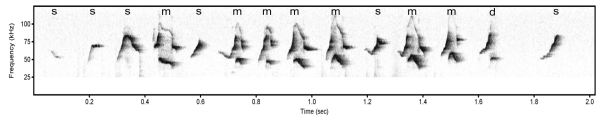
Figure 2: An example song segment sung by a wild type mouse under the U context.

The influences of social stimuli and genetic differences on mouse song syntax are also being extensively investigated. Chabout et al. (2012) studied the role of USVs in triggering and maintaining social interaction between male mice. Musolf et al. (2015) showed that the repertoire of male mice USVs differ among strains. Scattoni et al. (2008b) compared the USV repertoire in a strain of mouse that displays social abnormalities and repetitive behaviors analogous to symptoms of autism, with USVs produced by three other control strains. Chabout et al. (2015) studied if male mice change their syntax according to social contexts, exposing them to four different stimuli - fresh female urine on a cotton tip placed inside the male’s cage (U), awake and behaving adult female placed inside the cage (L), an anesthetized female placed on the lid of the cage (A), and anesthetized male placed on the lid of the cage (AM).

Chabout et al. (2016) investigated the effect of a rare mutation of the Foxp2 (forkhead-box P2) gene on the mouse vocalization patterns. Many human spoken language disorders are suspected to be caused by this mutation. Affected individuals have difficulties mastering the coordinated movement sequences of syllables that underlie fluent speech, described as developmental verbal dyspraxia (DVD) or childhood apraxia of speech (CAS), accompanied by other problems with verbal and written language. The Foxp2 orthologs’ coding sequences and brain expressions are remarkably conserved across species, including humans and mice (Lai et al., 2003; Haesler et al., 2004). It is thus interesting to explore if the mouse vocalization model can be used to gain insights into the role of Foxp2 in vocalization capabilities across the two mammalian species. To this end, Chabout et al. (2016) compared songs sung by mice carrying the mutation with songs produced by wild type mice under the female mouse related stimuli U, L and A. Other mouse vocalization experiments studying the role of Foxp2 include Fujita et al. (2008); Castellucci et al. (2016); Gaub et al. (2016) etc.

Notably, each of these data sets can be described as a collection of songs recorded under different combination of values of associated predictors. The data sets studied in Scattoni et al. (2008b); Fujita et al. (2008), for example, comprised songs produced by mice from different genotypes. The data sets studied in Chabout et al. (2012, 2015) consisted of songs recorded under different social stimuli. The data sets studied in Gaub et al. (2016); Chabout et al. (2016) comprised songs recorded under different combinations of genotype and context. Also, in all these studies, neuroscientists are primarily interested in assessing the global and local influences of the predictors on the mouse vocalization patterns and abilities.

Foxp2 Mutant
Mouse ID	Social Context
	U	L	A
F1	1423	4514	2107
F2	3741	4099	4639
F3	2516	5059	4610
F4	3812	3207	2641
F5	3947	4598	1833
F6	730	3812	4479
F7	3909	4806	2391
F8	3347	3482	3335

Wild Type
Mouse ID	Social Context
	U	L	A
W1	3787	6063	5246
W2	4189	4975	1540
W3	3453	4971	5085
W4	2460	1776	3771
W5	2817	4806	3445
W6	2489	4281	587

Table 1: General structure of the Foxp2 data set studied in Chabout et al. (2016). Each cell represents the number of syllables making up the corresponding song.

While the literature on mouse vocalization studies has already become substantial and is growing very rapidly, statistical methods for analysis of syntax differences have lagged behind. Neuroscientists have thus often focused only on repertoire differences, comparing the overall proportions of syllables between different combinations of exogenous predictors, but have largely ignored the problem of studying systematic differences in sequential arrangements of these syllables within songs (Scattoni et al., 2008b; Chabout et al., 2012; Musolf et al., 2015; Gaub et al., 2016).

The mixed effects Markov model proposed in this article aims to provide a sophisticated statistical framework for assessing syntax differences due to exogenous factors. While the methodology is readily applicable to all the studies described above, to illustrate its utility, we will focus specifically on the Foxp2 study reported in Chabout et al. (2016). The general structure of the Foxp2 data set is depicted in Table 1 where $42$ songs of various lengths sung by $8$ Foxp2 mutant mice and $6$ wild type mice were recorded under the contexts U, L and A. Independent analyses of the songs using higher order models (Sarkar and Dunson, 2016) were strongly indicative of first order Markovian dynamics. The hypothesis of primary scientific interest postulates the Foxp2 mutation to significantly affect the mouse vocalization patterns and abilities across all contexts. A hypothesis of secondary interest is that the vocalization patterns also vary significantly between contexts across genotypes. Additionally, if the global effect of the Foxp2 mutation turns out to be significant, we are interested in assessing how the mutation affects the vocalization patterns locally for each fixed social context.

3 Mixed Effects Markov Chains

Consider a collection of categorical sequences $\{y_{s,t}\}_{s=1,t=1}^{s_{0},T_{s}}$ with $y_{s,t}\in{\cal S}_{0}=\{1\dots,d_{0}\}$. Each sequence $s$ has, associated with it, $p$ exogenous categorical predictors $\{x_{s,j}\}_{j=1}^{p}$ with $x_{s,j}\in{\cal S}_{j}=\{1,\dots,d_{j}\}$. These exogenous predictors remain fixed over time for each sequence. The notations $y_{t},x_{j}$ sans the subscript $s$ will sometimes be used to refer collectively to $y_{s,t}$, $x_{s,j}$ and also to denote values taken by them. The probability of $y_{s,t}$ taking a value in ${\cal S}_{0}$ is assumed to depend on its immediate previous value $y_{s,t-1}$ and possibly also on the values taken by the associated exogenous predictors $\{x_{s,j}\}_{j=1}^{p}$, and is denoted by $P_{x_{s,1},\dots,x_{s,p}}(y_{s,t}\mid y_{s,t-1})$. We refer to such sequences as Markov Chains with Exogenous Predictors (MCEP). The dynamics of the $s^{th}$ sequence is thus governed by the model

$$(y_{s,t}\mid y_{s,t-1},x_{s,j},j=1,\dots,p)\sim$$

$$\hskip 28.45274pt\hbox{Mult}[\{1,\dots,d_{0}\},P_{x_{s,1},\dots,x_{s,p}}(1\mid y_{s,t-1}),\dots,P_{x_{s,1},\dots,x_{s,p}}(d_{0}\mid y_{s,t-1})].$$

Additionally, each sequence $s$ may also be associated with an individual $i_{s}=i$ drawn at random from a larger population of interest ${\cal I}$. The individual level transition probabilities, denoted by $P_{x_{1},\dots,x_{p}}^{(i)}(y_{t}\mid y_{t-1})$, may then be assumed to have been randomly drawn from a population of transition probabilities ${\cal P}=\{P_{x_{1},\dots,x_{p}}^{(i)}(y_{t}\mid y_{t-1}):i\in{\cal I}\}$ with mean transition probability parameters $P_{x_{1},\dots,x_{p}}(y_{t}\mid y_{t-1})$. The model for the process governing the evolution of the $s^{th}$ sequence is now modified as

$$(y_{s,t}\mid y_{s,t-1},x_{s,j},j=1,\dots,p,i_{s})\sim$$

$$\hskip 28.45274pt\hbox{Mult}[\{1,\dots,d_{0}\},P_{x_{s,1},\dots,x_{s,p}}^{(i_{s})}(1\mid y_{s,t-1}),\dots,P_{x_{s,1},\dots,x_{s,p}}^{(i_{s})}(d_{0}\mid y_{s,t-1})].$$

Key inferential goals include estimation of individual and population level transition probabilities, $P_{x_{1},\dots,x_{p}}^{(i)}(y_{t}\mid y_{t-1})$ and $P_{x_{1},\dots,x_{p}}(y_{t}\mid y_{t-1})$, and an assessment of the global and local influence of the predictors on these transition probabilities. The hypotheses of a global impact of the $j^{th}$ predictor correspond to

$$H_{0j}:P_{x_{1},\dots,x_{p}}^{(i)}(y_{t}\mid y_{t-1})~{}\text{does not vary with values of}~{}x_{j}~{}~{}~{}\text{vs}$$

$$H_{1j}:P_{x_{1},\dots,x_{p}}^{(i)}(y_{t}\mid y_{t-1})~{}\text{varies with varying values of}~{}x_{j}.$$

Local hypotheses instead correspond to pairwise comparisons between transition probabilities for two different levels of $x_{j}$.

In our motivating application, $i_{s}$ indexes the mouse under study, $y_{s,t}\in{\cal S}_{0}=\{d,m,s,u,x\}=\{1,2,3,4,5\}$ denotes the sequence of ‘syllables’ measuring the song dynamics, and there are two categorical predictors - genotype $x_{s,1}\in{\cal S}_{1}=\{F,W\}=\{1,2\}$ and context $x_{s,2}\in{\cal S}_{2}=\{U,L,A\}=\{1,2,3\}$. A key interest is in studying the impact of a mutation in the Foxp2 gene on vocalization patterns across different contexts.

Towards these goals, we first focus, in Section 3.1, on the simpler problem of developing a statistical framework for MCEPs that facilitates testing the significance of the exogenous predictors, ignoring any individual specific effect. The problem of modeling individual level transition probabilities incorporating individual specific random effects is then addressed in Section 3.2.

3.1 A Partition Model for MCEP

To model MCEPs, we construct a probabilistic partition of each ${\cal S}_{j}$ such that the values of $x_{j}$ that are clustered together have similar influences on the dynamics of $y_{s,t}$. Specifically, given a random partition ${\cal C}^{(j)}=\{{\cal C}_{\ell}^{(j)}\}$ of ${\cal S}_{j},j=1,\dots,p$, we model the stochastic evolution of $y_{s,t}$ as

$$(y_{s,t}\mid y_{s,t-1},x_{s,j}\in{\cal C}_{\ell_{j}}^{(j)},j=1,\dots,p)\sim$$

$$\hskip 28.45274pt\hbox{Mult}[\{1,\dots,d_{0}\},\lambda_{\ell_{1},\dots,\ell_{p}}^{\star}(1\mid y_{s,t-1}),\dots,\lambda_{\ell_{1},\dots,\ell_{p}}^{\star}(d_{0}\mid y_{s,t-1})],$$ (1)

where $\mbox{\boldmath$\lambda$}_{\ell_{1},\dots,\ell_{p}}^{\star}(\cdot\mid y_{t-1})=\{\lambda_{\ell_{1},\dots,\ell_{p}}^{\star}(1\mid y_{t-1}),\dots,\lambda_{\ell_{1},\dots,\ell_{p}}^{\star}(d_{0}\mid y_{t-1})\}^{\rm T}$ are probability vectors for each combination $(y_{t-1},\ell_{1},\dots,\ell_{p})$. Clearly, $1\leq\left|{\cal C}^{(j)}\right|\leq d_{j}$. When $\left|{\cal C}^{(j)}\right|=1$, all $d_{j}$ categories are clustered together, and hence the evolution of $y_{s,t}$ does not depend on the specific value taken by the associated $j^{th}$ predictor $x_{s,j}$. We will refer to this case as the null model ${\cal M}_{0j}$ corresponding to null hypothesis $H_{0j}$. At the other extreme, $\left|{\cal C}^{(j)}\right|=d_{j}$ so that each of the $d_{j}$ categories of $x_{j}$ has its own cluster.

Introducing latent cluster allocation variables, we can re-express (1) as

$$(y_{s,t}\mid y_{s,t-1},z_{j,x_{s,j}}=h_{j},j=1,\dots,p)\sim$$

$$\hskip 28.45274pt\hbox{Mult}[\{1,\dots,d_{0}\},\lambda_{h_{1},\dots,h_{p}}(1\mid y_{s,t-1}),\dots,\lambda_{h_{1},\dots,h_{p}}(d_{0}\mid y_{s,t-1})],$$

$$z_{j,\ell}\sim\hbox{Mult}[\{1,\dots,k_{j}\},\pi_{1}^{(j)},\dots,\pi_{k_{j}}^{(j)}],$$ (2)

where $\mbox{\boldmath$\lambda$}_{h_{1},\dots,h_{p}}(\cdot\mid y_{t-1})=\{\lambda_{h_{1},\dots,h_{p}}(1\mid y_{t-1}),\dots,\lambda_{h_{1},\dots,h_{p}}(d_{0}\mid y_{t-1})\}^{\rm T}$ are probability vectors for each combination $(y_{t-1},h_{1},\dots,h_{p})$, and $\{z_{j,\ell}\}_{j=1,\ell=1}^{p,d_{j}}$ index allocation of the $d_{j}$ observed categories of the $j^{th}$ predictor to $k_{j}$ latent categories, inducing a partition ${\cal C}^{(j)}$ of ${\cal S}_{j}$. Two categories $\ell_{1},\ell_{2}\in\{1,\dots,d_{j}\}$ will be clustered together iff $z_{j,\ell_{1}}=z_{j,\ell_{2}}$.

The above formulation allows the partition ${\cal C}^{(j)}$ to comprise at most $k_{j}$ sets. By allowing empty latent components, such hierarchical formulations define many-to-one mappings from the space of possible combinations of $z_{j,\ell}$ to the space of possible partitions. For example, with $d_{j}=4$ and $k_{j}=3$, $(z_{j,1},\dots,z_{j,4})=(1,1,1,3)$, $(z_{j,1},\dots,z_{j,4})=(2,2,2,1)$, $(z_{j,1},\dots,z_{j,4})=(3,3,3,2)$ all induce the same partition ${\cal C}^{(j)}=\{\{1,2,3\},\{4\}\}$ of $\{1,\dots,d_{j}\}$. Given $\{z_{j,\ell}\}_{\ell=1,j=1}^{d_{j},p}$ and the labeling schemes for the sets in the induced partitions $\{{\cal C}^{(j)}\}_{j=1}^{p}$, the $\mbox{\boldmath$\lambda$}_{\ell_{1},\dots,\ell_{p}}^{\star}$’s and the $\mbox{\boldmath$\lambda$}_{h_{1},\dots,h_{p}}$’s that are associated with the nonempty components are uniquely related. For example, with $p=2$, $(z_{1,1},\dots,z_{1,4})=(1,1,1,3)$ and $(z_{2,1},\dots,z_{2,3})=(2,2,1)$, inducing the partitions ${\cal C}^{(1)}=\{{\cal C}_{1}^{(1)},{\cal C}_{2}^{(1)}\}=\{\{1,2,3\},\{4\}\}$ and ${\cal C}^{(2)}=\{{\cal C}_{1}^{(2)},{\cal C}_{2}^{(2)}\}=\{\{1,2\},\{3\}\}$, $\mbox{\boldmath$\lambda$}_{1,1}^{\star}=\mbox{\boldmath$\lambda$}_{1,2}$, $\mbox{\boldmath$\lambda$}_{1,2}^{\star}=\mbox{\boldmath$\lambda$}_{1,1}$, $\mbox{\boldmath$\lambda$}_{2,1}^{\star}=\mbox{\boldmath$\lambda$}_{3,2}$ and $\mbox{\boldmath$\lambda$}_{2,2}^{\star}=\mbox{\boldmath$\lambda$}_{3,1}$.

Model specification is completed with priors for probability vectors $\mbox{\boldmath$\lambda$}_{h_{1},\dots,h_{p}}(\cdot\mid y_{s,t-1})$ and $\mbox{\boldmath$\pi$}^{(j)}=\{\pi_{1}^{(j)},\dots,\pi_{k_{j}}^{(j)}\}^{\rm T}$. It is natural to center the prior for the transition probability vectors $\mbox{\boldmath$\lambda$}_{h_{1},\dots,h_{p}}(\cdot\mid y_{t-1})$ around some $\mbox{\boldmath$\lambda$}_{0}(\cdot\mid y_{t-1})$, which captures the overall transition dynamics. In addition, some states in ${\cal C}^{(0)}$ may be preferred to others across levels of the predictors. Let $\mbox{\boldmath$\lambda$}_{00}=\{\lambda_{00}(1),\dots,\lambda_{00}(d_{0})\}^{\rm T}$ be a probability vector capturing such global behaviors. A natural prior for $\mbox{\boldmath$\lambda$}_{h_{1},\dots,h_{p}}(\cdot\mid y_{t-1})$ that allows sharing of information across different layers of hierarchy may be specified as

$$\mbox{\boldmath$\lambda$}_{h_{1},\dots,h_{p}}(\cdot\mid y_{t-1})\sim\hbox{Dir}\{\alpha_{0}\lambda_{0}(1\mid y_{t-1}),\dots,\alpha_{0}\lambda_{0}(d_{0}\mid y_{t-1})\},$$

$$\mbox{\boldmath$\lambda$}_{0}(\cdot\mid y_{t-1})\sim\hbox{Dir}\{\alpha_{00}\lambda_{00}(1),\dots,\alpha_{00}\lambda_{00}(d_{0})\},~{}~{}~{}~{}~{}~{}\alpha_{0}\sim\hbox{Ga}(a_{\alpha_{0}},b_{\alpha_{0}}).$$

Likewise, a natural choice for the prior on $\mbox{\boldmath$\pi$}^{(j)}$ is given by $\mbox{\boldmath$\pi$}^{(j)}\sim\hbox{Dir}(\alpha_{j},\dots,\alpha_{j}).$ Marginalizing out $\mbox{\boldmath$\pi$}^{(j)}$, the induced prior on ${\cal C}^{(j)}=\{{\cal C}_{1}^{(j)},\dots,{\cal C}_{\widetilde{k}_{j}}^{(j)}\}$ is given by

$$p_{0}({\cal C}^{(j)})=\frac{{k_{j}}_{\left(\left|{\cal C}^{(j)}\right|\right)}}{(k_{j}\alpha_{j})^{(d_{j})}}\prod_{\ell_{j}=1}^{\left|{\cal C}^{(j)}\right|}\alpha_{j}^{\left(\left|{\cal C}_{\ell_{j}}^{(j)}\right|\right)},$$

where $x^{(i)}=x(x+1)\cdots(x+m-1)$ and $x_{(m)}=x(x-1)\cdots(x-m+1)$. The prior probability of the null model ${\cal M}_{0j}$ is then obtained as

$$p_{0}({\cal M}_{0j})=p_{0}(\widetilde{k}_{j}=1)={k_{j}\alpha_{j}^{(d_{j})}}/{(k_{j}\alpha_{j})^{(d_{j})}}.$$

Since $1\leq\left|{\cal C}^{(j)}\right|\leq d_{j}$, a nonparametric partition model is obtained by setting $k_{j}=d_{j}$, with $\alpha_{j}=\alpha/k_{j}$, which converges weakly to a Dirichlet process as $k_{j}\to\infty$.

Our proposed model is related to the rich literature on reducing dimensionality in characterizing predictor effects via partitioning; refer, for example to Breiman et al. (1984); Denison et al. (1998), though we are not aware of such methods being developed in the setting of characterizing predictor effects on Markov dynamics.

3.2 Mixed Effects MCEP

Having developed a general framework for MCEP, we now address the problem of incorporating individual effects into the model. For ease of exposition and interpretation, we focus initially on settings similar to our motivating application of mouse vocalization experiments. Extensions to similar other scenarios are straightforward.

In our motivating application, we have $m=1,\dots,m_{x_{1}}$ mice from genotypes $x_{1}\in{\cal S}_{1}=\{1,\dots,d_{1}\}$ singing under contexts $x_{2}\in{\cal S}_{2}=\{1,\dots,d_{2}\}$, generating a total of $s_{0}=d_{2}\sum_{x_{1}=1}^{d_{1}}m_{x_{1}}$ songs $\{y_{s,t}\}_{s=1,t=1}^{s_{0},T_{s}}$. The model developed in Section 3.1 assumes that under a given context all $m_{x_{1}}$ mice from the $x_{1}^{th}$ genotype sing according to the same probability model. Introducing mouse-specific transition distributions $\mbox{\boldmath$\lambda$}^{(i)}(\cdot\mid y_{t-1})=\{\lambda^{(i)}(1\mid y_{t-1}),\dots,\lambda^{(i)}(d_{0}\mid y_{t-1})\}^{\rm T}$, we characterize the transition dynamics of the different mice according to the hierarchical model

$$(y_{s,t}\mid y_{s,t-1},i_{s}=i,z_{j,x_{s,j}}=h_{j},j=1,2)\sim$$

$$\hskip 28.45274pt\hbox{Mult}[\{1,\dots,d_{0}\},P_{h_{1},h_{2}}^{(i)}(1\mid y_{s,t-1}),\dots,P_{h_{1},h_{2}}^{(i)}(d_{0}\mid y_{s,t-1})],~{}~{}\text{where}$$

$${\mathbf{P}}_{h_{1},h_{2}}^{(i)}(\cdot\mid y_{t-1})=\pi_{0}(y_{t-1})\mbox{\boldmath$\lambda$}_{h_{1},h_{2}}(\cdot\mid y_{t-1})+\pi_{1}(y_{t-1})\mbox{\boldmath$\lambda$}^{(i)}(\cdot\mid y_{t-1}),$$

$$z_{j,\ell}\sim\hbox{Mult}[\{1,\dots,d_{j}\},\pi_{1}^{(j)},\dots,\pi_{d_{j}}^{(j)}],~{}~{}~{}~{}~{}~{}~{}~{}~{}~{}~{}\mbox{\boldmath$\pi$}^{(j)}\sim\hbox{Dir}(\alpha_{j},\dots,\alpha_{j}),$$

$$\mbox{\boldmath$\lambda$}^{(i)}(\cdot\mid y_{t-1})\sim\hbox{Dir}\{\alpha^{(0)}\lambda_{0}(1\mid y_{t-1}),\dots,\alpha^{(0)}\lambda_{0}(d_{0}\mid y_{t-1})\},$$

$$\mbox{\boldmath$\lambda$}_{h_{1},h_{2}}(\cdot\mid y_{t-1})\sim\hbox{Dir}\{\alpha_{0}\lambda_{0}(1\mid y_{t-1}),\dots,\alpha_{0}\lambda_{0}(d_{0}\mid y_{t-1})\},$$

$$\mbox{\boldmath$\lambda$}_{0}(\cdot\mid y_{t-1})\sim\hbox{Dir}\{\alpha_{00}\lambda_{00}(1),\dots,\alpha_{00}\lambda_{00}(d_{0})\},$$

$$\pi_{0}(y_{t-1})\sim\hbox{Beta}(a_{0},a_{1}),~{}~{}~{}~{}~{}~{}\alpha_{0}\sim\hbox{Ga}(a_{\alpha_{0}},b_{\alpha_{0}}),~{}~{}~{}~{}~{}~{}~{}\alpha^{(0)}\sim\hbox{Ga}(a_{\alpha^{(0)}},b_{\alpha^{(0)}}).$$ (3)

Expression (3) characterizes the mouse-specific transition probability ${\mathbf{P}}_{h_{1},h_{2}}^{(i)}(\cdot\mid y_{t-1})$ as a convex combination of a baseline probability $\mbox{\boldmath$\lambda$}_{h_{1},h_{2}}(\cdot\mid y_{t-1})$ and a mouse-specific random effect $\mbox{\boldmath$\lambda$}^{(i)}(\cdot\mid y_{t-1})$, with respective weights $\pi_{0}(y_{t-1})$ and $\pi_{1}(y_{t-1})=1-\pi_{0}(y_{t-1})$. The baseline component is common to all mice from genotype $x_{1}$ with $z_{1,x_{1}}=h_{1}$ singing under context $x_{2}$ with $z_{2,x_{2}}=h_{2}$, and provides a type of fixed effects term. The probability $\pi_{1}(y_{t-1})$ characterizes the amount of heterogeneity among mice, taking the place of the random effects variance in a traditional mixed effects model. The convex structure facilitates computation and interpretability.

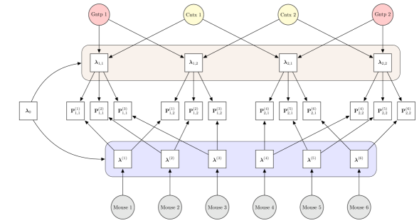
Figure 3: Graphical model showing information sharing for sequences with similar predictors and/or from the same mouse. Predictors include genotype $\in\{\mbox{Gntp 1, Gntp 2}\}$ and context $\in\{\mbox{Cntx 1, Cntx 2}\}$. Mice 1-3 have Gntp 1, Mice 4-6 have Gntp 2. Brown shading = predictor effects, Blue shading = random effects.

Figure 3 shows how the proposed formulation shares information across songs associated with the same levels of genotype and context as well as across songs sung by the same mouse. The convex form of the model is interpretable as a two-component mixture of a global and local component. Related global-local mixtures have been proposed in fundamentally different contexts by Müller et al. (2004), Dunson (2006) and Ren et al. (2010).

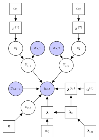
Figure 4: Pictorial representation of the local dependency structure in a sequence $\{y_{s,t}\}$ produced by the $i_{s}^{th}$ individual with two exogenous predictors $x_{s,1}$ and $x_{s,2}$. Observed and latent variables are marked by shaded and unshaded nodes, respectively.

3.3 Model Properties

Switching back to general settings with $p$ exogenous predictors, we have

$${\mathbf{P}}_{h_{1},\dots,h_{p}}^{(i)}(\cdot\mid y_{t-1})=\pi_{0}(y_{t-1})\mbox{\boldmath$\lambda$}_{h_{1},\dots,h_{p}}(\cdot\mid y_{t-1})+\pi_{1}(y_{t-1})\mbox{\boldmath$\lambda$}^{(i)}(\cdot\mid y_{t-1}).$$

Introducing latent variables $v_{s,t}\in\{0,1\}$ for each $y_{s,t}$, we can write

$$\{y_{s,t}\mid y_{s,t-1},i_{s}=i,z_{j,x_{s,j}}=h_{j},j=1,\dots,p,v_{s,t}\}\sim$$

$$\hskip 28.45274pt\left\{\begin{array}[]{lc}\hbox{Mult}[\{1,\dots,d_{0}\},\lambda^{(i)}(1\mid y_{s,t-1}),\dots,\lambda^{(i)}(d_{0}\mid y_{s,t-1})]&\text{if}~{}v_{s,t}=0,\\ \hbox{Mult}[\{1,\dots,d_{0}\},\lambda_{h_{1},h_{2}}(1\mid y_{s,t-1}),\dots,\lambda_{h_{1},h_{2}}(d_{0}\mid y_{s,t-1})]&\text{if}~{}v_{s,t}=1,\\ \end{array}\right.$$

$$(v_{s,t}=\ell\mid y_{s,t-1})\sim\hbox{Mult}[\{0,1\},\pi_{0}(y_{s,t-1}),\pi_{1}(y_{s,t-1})].$$

Sampling the $v_{s,t}$’s facilitates posterior computation. A graphical model characterization is shown in Figure 4.

Conditioning on $\mbox{\boldmath$\lambda$}_{0}$, an alternative representation of ${\mathbf{P}}_{h_{1},\dots,h_{p}}^{(i)}(\cdot\mid y_{t-1})$ is obtained after some simple algebraic manipulation as

$${\mathbf{P}}_{h_{1},\dots,h_{p}}^{(i)}(\cdot\mid y_{t-1})=\mbox{\boldmath$\lambda$}_{0}(\cdot\mid y_{t-1})+\pi_{0}(y_{t-1})\{\mbox{\boldmath$\lambda$}_{h_{1},\dots,h_{p}}(\cdot\mid y_{t-1})-\mbox{\boldmath$\lambda$}_{0}(\cdot\mid y_{t-1})\}$$

$$~{}~{}~{}~{}~{}~{}~{}~{}~{}~{}~{}~{}~{}~{}~{}~{}~{}~{}~{}~{}~{}~{}~{}~{}~{}~{}~{}~{}~{}~{}~{}~{}~{}~{}~{}~{}~{}+\pi_{1}(y_{t-1})\{\mbox{\boldmath$\lambda$}^{(i)}(\cdot\mid y_{t-1})-\mbox{\boldmath$\lambda$}_{0}(\cdot\mid y_{t-1})\}.$$

With $\mbox{\boldmath$\lambda$}_{h_{1},\dots,h_{p}}(\cdot\mid y_{t-1})$ and $\mbox{\boldmath$\lambda$}^{(i)}(\cdot\mid y_{t-1})$ distributed around $\mbox{\boldmath$\lambda$}_{0}(\cdot\mid y_{t-1})$, the expressions within the braces above are centered around zero. The first term is interpreted as the global mean, the second term as the departure from the global mean due to the fixed effects, and the final term as departure due to individual-specific random effects. Integrating out $\mbox{\boldmath$\lambda$}^{(i)}(\cdot\mid y_{t-1})$, the transition probability vectors ${\mathbf{P}}_{h_{1},\dots,h_{p}}^{(i)}(\cdot\mid y_{t-1})$ are centered around their population mean

$${\mathbf{P}}_{h_{1},\dots,h_{p}}(\cdot\mid y_{t-1})=\mbox{\boldmath$\lambda$}_{0}(\cdot\mid y_{t-1})+\pi_{0}(y_{t-1})\{\mbox{\boldmath$\lambda$}_{h_{1},\dots,h_{p}}(\cdot\mid y_{t-1})-\mbox{\boldmath$\lambda$}_{0}(\cdot\mid y_{t-1})\}.$$

Unlike nonlinear GLM based approaches, our proposed formulation results in closed form expressions for the population level transition probabilities with the fixed effects terms having the same individual and population level interpretations. Also, importantly, the population level probability parameters do not depend on the variability of the subject-specific effects. These advantages over GLM based approaches are discussed in greater detail in Section S.3 in the Supplementary Materials.

The hyper-parameters $\alpha_{0}$ and $\alpha^{(0)}$ control the variability of $\mbox{\boldmath$\lambda$}_{h_{1},\dots,h_{p}}$ and $\mbox{\boldmath$\lambda$}^{(i)}$ around their means. Treating these parameters to be unknown and inferring them from their posterior makes the proposed approach more data adaptive. For the fixed effects components $\mbox{\boldmath$\lambda$}_{h_{1},\dots,h_{p}}$, we have

$$\hbox{var}\{\lambda_{h_{1},\dots,h_{p}}(y_{t}\mid y_{t-1})\mid\alpha_{0},\lambda_{0}(y_{t}\mid y_{t-1})\}=\lambda_{0}(y_{t}\mid y_{t-1})\{1-\lambda_{0}(y_{t}\mid y_{t-1})\}(\alpha_{0}+1)^{-1}.$$

In the limit, when $\alpha_{0}\to\infty$, $\hbox{var}\{\lambda_{h_{1},\dots,h_{p}}(y_{t}\mid y_{t-1})\mid\alpha_{0},\lambda_{0}(y_{t}\mid y_{t-1})\}\to 0$. The limiting case $\pi_{0}(y_{t-1})\to 0$ for all $y_{t-1}\in{\cal S}_{0}$ also signifies the absence of fixed effects. Likewise, for the random effects components, we have

$$\hbox{var}\{\lambda^{(i)}(y_{t}\mid y_{t-1})\mid\alpha^{(0)},\lambda_{0}(y_{t}\mid y_{t-1})\}=\lambda_{0}(y_{t}\mid y_{t-1})\{1-\lambda_{0}(y_{t}\mid y_{t-1})\}(\alpha^{(0)}+1)^{-1}.$$

In the limit, when $\alpha^{(0)}\to\infty$, $\hbox{var}\{\lambda^{(i)}(y_{t}\mid y_{t-1})\mid\alpha^{(0)},\lambda_{0}(y_{t}\mid y_{t-1})\}\to 0$. Random effects are also absent when $\pi_{1}(y_{t-1})\to 0$ for all $y_{t-1}\in{\cal S}_{0}$. If interest lies in testing the presence or absence of random effects, the prior for $\mbox{\boldmath$\lambda$}^{(i)}(\cdot\mid y_{t-1})$ can be adapted to include a point mass at $\mbox{\boldmath$\lambda$}_{0}(\cdot\mid y_{t-1})$.

The correlation structure between transition probabilities for different levels of the predictors and individuals provides further insights into the information sharing properties of the proposed model. For $(h_{11},\dots,h_{1p})\neq(h_{21},\dots,h_{2p})$, we have

$$\rho^{(i)} = \hbox{corr}\{P_{h_{11},\dots,h_{1p}}^{(i)}(y_{t}\mid y_{t-1}),P_{h_{21},\dots,h_{2p}}^{(i)}(y_{t}\mid y_{t-1})\mid\lambda_{0}(y_{t}\mid y_{t-1}),\pi_{0}(y_{t-1}),\alpha_{0},\alpha^{(0)}\}$$

$$= \frac{\pi_{1}^{2}(y_{t-1})/(\alpha^{(0)}+1)}{\{\pi_{0}^{2}(y_{t-1})/(\alpha_{0}+1)+\pi_{1}^{2}(y_{t-1})/(\alpha^{(0)}+1)\}}.$$

Likewise, for $i_{1}\neq i_{2}$, we have

$$\rho^{(i_{1},i_{2})} = \hbox{corr}\{P_{h_{1},\dots,h_{p}}^{(i_{1})}(y_{t}\mid y_{t-1}),P_{h_{1},\dots,h_{p}}^{(i_{2})}(y_{t}\mid y_{t-1})\mid\lambda_{0}(y_{t}\mid y_{t-1}),\pi_{0}(y_{t-1}),\alpha_{0},\alpha^{(0)}\}$$

$$= \frac{\pi_{0}^{2}(y_{t-1})/(\alpha_{0}+1)}{\{\pi_{0}^{2}(y_{t-1})/(\alpha_{0}+1)+\pi_{1}^{2}(y_{t-1})/(\alpha^{(0)}+1)\}}.$$

Finally, for $(h_{11},\dots,h_{1p})\neq(h_{21},\dots,h_{2p})$ and $i_{1}\neq i_{2}$, we have

$$\hbox{corr}\{P_{h_{11},\dots,h_{1p}}^{(i_{1})}(y_{t}\mid y_{t-1}),P_{h_{21},\dots,h_{2p}}^{(i_{2})}(y_{t}\mid y_{t-1})\mid\lambda_{0}(y_{t}\mid y_{t-1}),\pi_{0}(y_{t-1}),\alpha_{0},\alpha^{(0)}\}=0.$$

These expressions are all independent of the mean $\lambda_{0}(y_{t}\mid y_{t-1})$. If $\{\pi_{0}^{2}(y_{t-1})(\alpha^{(0)}+1)\}/\{\pi_{1}^{2}(y_{t-1})(\alpha_{0}+1)\}\to 0$, $\rho^{(i)}\to 1$. Conversely, if $\{\pi_{0}^{2}(y_{t-1})(\alpha^{(0)}+1)\}/\{\pi_{1}^{2}(y_{t-1})(\alpha_{0}+1)\}\to\infty$, $\rho^{(i)}\to 0$ . If $\{\pi_{0}^{2}(y_{t-1})(\alpha^{(0)}+1)\}/\{\pi_{1}^{2}(y_{t-1})(\alpha_{0}+1)\}\to 0$, $\rho^{(i_{1},i_{2})}\to 0$, and, conversely, if $\{\pi_{0}^{2}(y_{t-1})(\alpha^{(0)}+1)\}/\{\pi_{1}^{2}(y_{t-1})(\alpha_{0}+1)\}\to\infty$, $\rho^{(i_{1},i_{2})}\to 1$. Without the random effect components, we would have had $\rho^{(i)}=0$ and $\rho^{(i_{1},i_{2})}=1$.

Supplementary Materials contain further details on some properties of our proposed model, including ergodicity, flexibility and posterior consistency. As the model is effectively nonparametric, we can show that the transition probabilities for each of the subjects are estimated consistently as the length of each sequence increases. This seems to be the appropriate asymptotic notion in our motivating application, as it is easy to collect more data on mice but practically impossible to study more than a small to moderate number of mice.

4 Posterior Inference

4.1 Posterior Computation

Inference is based on samples drawn from the posterior using a Gibbs sampler that exploits the conditional independence relationships depicted in Figure 4. In what follows, $\zeta$ denotes a generic variable that collects all other variables not explicitly mentioned, including the data points. The sampler comprises the following steps.

1. Sample each $z_{j,\ell}$ according to its multinomial full conditional

   $$p(z_{j,\ell}=h_{j}\mid z_{j^{\prime},\ell}=h_{j^{\prime}},j^{\prime}\neq j,\mbox{\boldmath$\zeta$})\propto\pi_{h_{j}}^{(j)}\times$$

   $$\prod_{y_{t-1}}\prod_{(h_{1},\dots,h_{p})}\frac{\beta\{\alpha_{0}\lambda_{0}(1\mid y_{t-1})+n_{h_{1},\dots,h_{p}}(1\mid y_{t-1}),\dots,\alpha_{0}\lambda_{0}(d_{0}\mid y_{t-1})+n_{h_{1},\dots,h_{p}}(d_{0}\mid y_{t-1})\}}{\beta\{\alpha_{0}\lambda_{0}(1\mid y_{t-1}),\dots,\alpha_{0}\lambda_{0}(d_{0}\mid y_{t-1})\}},$$

   where $n_{h_{1},\dots,h_{p}}(y_{t}\mid y_{t-1})=\sum_{s,t}1\{y_{s,t}=y_{t},y_{s,t-1}=y_{t-1},v_{s,t}=0,z_{j,x_{s,j}}=h_{j},j=1,\dots,p\}$.

2. Sample each $\mbox{\boldmath$\pi$}^{(j)}$ according to its Dirichlet full conditional

   $$\{\pi^{(j)}(1),\dots,\pi^{(j)}(d_{j})\}\mid\mbox{\boldmath$\zeta$}\sim\hbox{Dir}\{\alpha_{j}+n_{j}(1),\dots,\alpha_{j}+n_{j}(d_{j})\},$$

   where $n_{j}(h)=\sum_{\ell=1}^{d_{j}}1\{z_{j,\ell}=h\}$.

3. Sample each $v_{s,t}$ according to its Bernoulli full conditional

   $$p(v_{s,t}=v\mid\mbox{\boldmath$\zeta$})\propto\pi_{v}(y_{s,t-1})\times\widetilde{\lambda}_{v}(y_{s,t}\mid y_{s,t-1}),$$

   where $\widetilde{}\mbox{\boldmath$\lambda$}_{0}(\cdot\mid y_{t-1})=\mbox{\boldmath$\lambda$}_{h_{1},\dots,h_{p}}(\cdot\mid y_{t-1})$ with $(z_{1,x_{s,1}},\dots,z_{p,x_{s,p}})=(h_{1},\dots,h_{p})$, and $\widetilde{}\mbox{\boldmath$\lambda$}_{1}(\cdot\mid y_{t-1})=\mbox{\boldmath$\lambda$}^{(i)}(\cdot\mid y_{t-1})$.

4. Sample $\mbox{\boldmath$\pi$}=\{\pi_{0}(y_{t-1}),\pi_{1}(y_{t-1})\}^{\rm T}$ according to its Beta full conditional

   $$\{\pi_{0}(y_{t-1}),\pi_{1}(y_{t-1})\}\mid\mbox{\boldmath$\zeta$}\sim\hbox{Beta}\{a_{0}+n_{0}(y_{t-1}),a_{1}+n_{1}(y_{t-1})\},$$

   where $n_{v}(y_{t-1})=\sum_{s,t}1\{v_{s,t}=v,y_{s,t-1}=y_{t-1}\}$.

5. Sample each $\mbox{\boldmath$\lambda$}^{(i)}(\cdot\mid y_{t-1})$’s according to its Dirichlet full conditional

   $$\{\lambda^{(i)}(1\mid y_{t-1}),\dots,\lambda^{(i)}(d_{0}\mid y_{t-1})\}\mid\mbox{\boldmath$\zeta$}\sim$$

   $$\hbox{Dir}\{\alpha^{(0)}\lambda_{0}(1\mid y_{t-1})+n^{(i)}(1\mid y_{t-1}),\dots,\alpha^{(0)}\lambda_{0}(d_{0}\mid y_{t-1})+n^{(i)}(d_{0}\mid y_{t-1})\},$$

   where $n^{(i)}(y_{t}\mid y_{t-1})=\sum_{s,t}1\{y_{s,t}=y_{t},y_{s,t-1}=y_{t-1},v_{s,t}=1,i_{s}=i\}$.

6. Sample each $\mbox{\boldmath$\lambda$}_{h_{1},\dots,h_{p}}(\cdot\mid y_{t-1})$ according to its Dirichlet full conditional

   $$\{\lambda_{h_{1},\dots,h_{p}}(1\mid y_{t-1}),\dots,\lambda_{h_{1},\dots,h_{p}}(d_{0}\mid y_{t-1})\}\mid\mbox{\boldmath$\zeta$}\sim$$

   $$\hbox{Dir}\{\alpha_{0}\lambda_{0}(1\mid y_{t-1})+n_{h_{1},\dots,h_{p}}(1\mid y_{t-1}),\dots,\alpha_{0}\lambda_{0}(d_{0}\mid y_{t-1})+n_{h_{1},\dots,h_{p}}(d_{0}\mid y_{t-1})\}.$$

7. Let $v_{h_{1},\dots,h_{p}}(y_{t}\mid y_{t-1})=0$ and $n=0$. Sample an auxiliary variable $\xi$ as

   $$\xi\mid\mbox{\boldmath$\zeta$}\sim\hbox{Bernoulli}\left\{\frac{\alpha_{0}\lambda_{0}(y_{t}\mid y_{t-1})}{n+\alpha_{0}\lambda_{0}(y_{t}\mid y_{t-1})}\right\}.$$

   Set $n=n+1$ and $v_{h_{1},\dots,h_{p}}(y_{t}\mid y_{t-1})=v_{h_{1}\dots,h_{p}}(y_{t}\mid y_{t-1})+\xi$. Continue until $n$ equals $n_{h_{1},\dots,h_{p}}(y_{t}\mid y_{t-1})$. Likewise, set $v^{(i)}(y_{t}\mid y_{t-1})=0$ and $n=0$. Sample an auxiliary variable $\xi$ as

   $$\xi\mid\mbox{\boldmath$\zeta$}\sim\hbox{Bernoulli}\left\{\frac{\alpha^{(0)}\lambda_{0}(y_{t}\mid y_{t-1})}{n+\alpha^{(0)}\lambda_{0}(y_{t}\mid y_{t-1})}\right\}.$$

   Set $n=n+1$ and $v^{(i)}(y_{t}\mid y_{t-1})=v^{(i)}(y_{t}\mid y_{t-1})+\xi$. Continue until $n$ equals $n^{(i)}(y_{t}\mid y_{t-1})$. Set $v(y_{t}\mid y_{t-1})=\sum_{h_{1},\dots,h_{p}}v_{h_{1},\dots,h_{p}}(y_{t}\mid y_{t-1})+\sum_{i}v^{(i)}(y_{t}\mid y_{t-1})$. Also, set $v_{0}=\sum_{y_{t}}\sum_{y_{t-1}}\sum_{h_{1},\dots,h_{p}}v_{h_{1},\dots,h_{p}}(y_{t}\mid y_{t-1})$, and $v^{(0)}=\sum_{y_{t}}\sum_{y_{t-1}}\sum_{h_{1},\dots,h_{p}}v^{(i)}(y_{t}\mid y_{t-1})$. Additionally, sample auxiliary variables

   $$r_{h_{1},\dots,h_{p}}(y_{t-1})\mid\mbox{\boldmath$\zeta$}\sim\hbox{Beta}\{\alpha_{0}+1,n_{h_{1},\dots,h_{p}}(y_{t-1})\},$$

   $$s_{h_{1},\dots,h_{p}}(y_{t-1})\mid\mbox{\boldmath$\zeta$}\sim\hbox{Bernoulli}\left\{\frac{n_{h_{1},\dots,h_{p}}(y_{t-1})}{n_{h_{1},\dots,h_{p}}(y_{t-1})+\alpha_{0}}\right\},$$

   $$r^{(i)}(y_{t-1})\mid\mbox{\boldmath$\zeta$}\sim\hbox{Beta}\{\alpha^{(0)}+1,n^{(i)}(y_{t-1})\},$$

   $$s^{(i)}(y_{t-1})\mid\mbox{\boldmath$\zeta$}\sim\hbox{Bernoulli}\left\{\frac{n^{(i)}(y_{t-1})}{n^{(i)}(y_{t-1})+\alpha^{(0)}}\right\},$$

   where $n_{h_{1},\dots,h_{p}}(y_{t-1})=\sum_{y_{t}}n_{h_{1},\dots,h_{p}}(y_{t}\mid y_{t-1})$ and $n^{(i)}(y_{t-1})=\sum_{y_{t}}n^{(i)}(y_{t}\mid y_{t-1})$. Set $\hbox{log}~{}r_{0}=\sum_{y_{t-1}}\sum_{h_{1},\dots,h_{p}}\hbox{log}~{}r_{h_{1},\dots,h_{p}}(y_{t-1})$, $s_{0}=\sum_{y_{t-1}}\sum_{h_{1},\dots,h_{p}}s_{h_{1},\dots,h_{p}}(y_{t-1})$, $\hbox{log}~{}r^{(0)}=\sum_{y_{t-1}}\sum_{i}\hbox{log}~{}r^{(i)}(y_{t-1})$, and $s^{(0)}=\sum_{y_{t-1}}\sum_{m}s^{(i)}(y_{t-1})$.

8. Sample $\alpha_{0}$ according to its Gamma full conditional

   $$\alpha_{0}\mid\mbox{\boldmath$\zeta$}\sim\hbox{Ga}(a_{\alpha_{0}}+v_{0}-s_{0},b_{\alpha_{0}}-\hbox{log}~{}r_{0}).$$

9. Sample $\alpha^{(0)}$ according to its Gamma full conditional

   $$\alpha^{(0)}\mid\mbox{\boldmath$\zeta$}\sim\hbox{Ga}(a_{\alpha^{(0)}}+v^{(0)}-s^{(0)},b_{\alpha^{(0)}}-\hbox{log}~{}r^{(0)}).$$

10. Finally, sample $\mbox{\boldmath$\lambda$}_{0}$ according to its Dirichlet full conditional

    $$\{\lambda_{0}(1\mid y_{t-1}),\dots,\lambda_{0}(d_{0}\mid y_{t-1})\}\mid\mbox{\boldmath$\zeta$}\sim$$

    $$\hbox{Dir}\{\alpha_{00}\lambda_{00}(1)+v(1\mid y_{t-1}),\dots,\alpha_{00}\lambda_{00}(d_{0})+v(d_{0}\mid y_{t-1})\}.$$

The steps to update the hyper-parameters $\alpha_{0}$, $\alpha^{(0)}$ and the global transition distributions $\mbox{\boldmath$\lambda$}_{0}$ were adapted from the auxiliary variable sampler of West (1992) and Teh et al. (2006). In all our examples, $5,000$ MCMC iterations with the initial $2,000$ discarded as burn-in and the remaining samples thinned by an interval of $5$ produced very stable estimates of the individual and population level parameters of interest. MCMC diagnostic checks were not indicative of any convergence or mixing issues. Our implementation is fully automated, taking in only a single matrix argument - concatenated sequences $y_{s,t}$ with the associated values of the exogenous predictors $x_{s,j}$ and the subject labels repeated $T_{s}$ times for each sequence $s$ and included as additional columns. For the Foxp2 data set, this required feeding a $148778\times 4$ dimensional data matrix to the codes and $5,000$ MCMC iterations required approximately two hours to run on an ordinary laptop.

4.2 Prior Hyper-parameters and MCMC Initializations

In all our examples, real or synthetic, we set $\alpha_{00}=1$ and $\lambda_{00}(y_{t})=\sum_{s,t}1\{y_{s,t}=y_{t}\}/\sum_{s}T_{s}$, the overall proportion of syllables among all songs. We set each $\alpha_{j}$ at the value for which $p_{0}(H_{0j})=p_{0}(\widetilde{k}_{j}=1)=1/2$. For $j=1,\dots,p$, we initialize $\mbox{\boldmath$\pi$}^{(j)}$ at $(1/d_{j},\dots,1/d_{j})^{\rm T}$. We initialize each $z_{j,h}$ at $h$ for $h=1,\dots,d_{j}$. Each level of $x_{j}$ thus initially forms its own cluster. The associated $\mbox{\boldmath$\lambda$}_{h_{1},\dots,h_{p}}(y_{t}\mid y_{t-1})$ are initialized at $\sum_{s,t}1\{y_{s,t}=y_{t},y_{s,t-1}=y_{t-1},x_{s,j}=h_{j},j=1,\dots,p\}/\sum_{s,t}1\{y_{s,t-1}=y_{t-1},x_{s,j}=h_{j},j=1,\dots,p\}$. Likewise, $\mbox{\boldmath$\lambda$}^{(i)}(y_{t}\mid y_{t-1})$ are initialized at $\sum_{s,t}1\{y_{s,t}=y_{t},y_{s,t-1}=y_{t-1},i_{s}=i\}/\sum_{s,t}1\{y_{s,t-1}=y_{t-1},i_{s}=i\}$. For each $y_{t-1}$, $\{\pi_{0}(y_{t-1}),\pi_{1}(y_{t-1})\}$ is initialized at $(0.8,0.2)$. The $v_{s,t}$’s are initialized by sampling from Bernoulli distribution with parameter $\pi_{0}(y_{s,t-1})$. The parameters $\alpha_{0}$ and $\alpha^{(0)}$ are both initialized at $1$. For the remaining fixed hyper-parameters, we set $a=b=a_{\alpha_{0}}=b_{\alpha_{0}}=a_{\alpha^{(0)}}=b_{\alpha^{(0)}}=1$. Extensive experiments suggested the results to be highly robust to these choices.

4.3 Assessment of Global and Local Differences

Following Section 3.1, $\widetilde{k}_{j}>1$ if and only if $H_{1j}$ is true, so that the posterior probability of $H_{1j}$ can be estimated simply as the proportion of Gibbs sampling draws for which $\widetilde{k}_{j}>1$. If there is substantial evidence in favor of $H_{1j}$, it is typically of additional interest to conduct pairwise comparisons. For example, in the Foxp2 data set, if the effects of genotype $x_{1}$ are significant, interest lies in assessing the differences between $P_{1,x_{2}}(y_{t}\mid y_{t-1})$ and $P_{2,x_{2}}(y_{t}\mid y_{t-1})$ locally for each $(y_{t},y_{t-1})\in{\cal S}_{0}^{2}$ for each fixed context $x_{2}\in{\cal S}_{2}$. In particular, we consider the local tests $H_{0,y_{t}\mid y_{t-1},x_{2}}:\left|\Delta P_{\cdot,x_{2}}(y_{t}\mid y_{t-1})\right|=|P_{1,x_{2}}(y_{t}\mid y_{t-1})-P_{2,x_{2}}(y_{t}\mid y_{t-1})|\leq\delta$ vs $H_{1,y_{t}\mid y_{t-1},x_{2}}:\left|\Delta P_{\cdot,x_{2}}(y_{t}\mid y_{t-1})\right|>\delta$ for different $(y_{t},y_{t-1})\in{\cal S}_{0}^{2}$ and $x_{2}\in{\cal S}_{2}$, with $\delta$ a small constant elicited to correspond to a ‘practically’ significant difference. The posterior probabilities of these local tests can be easily estimated from the output of the Gibbs sampler.

5 Application to the Foxp2 Data Set

In this section, we discuss the results of the proposed methodology applied to the Foxp2 data set. Our inference goals focus on studying the systematic variation in the mouse song dynamics across genotypes and contexts, with it being of additional substantial interest to assess the magnitude of unexplained variation among mice.

Figure 6 shows the estimated posterior mean transition probabilities $P_{x_{1},x_{2}}(y_{t}\mid y_{t-1})$, Figures S.1 and S.3 in the Supplementary Materials summarize the posterior standard deviations of $P_{x_{1},x_{2}}(y_{t}\mid y_{t-1})$ and the random effects parameters $\pi_{1}(y_{t-1})\lambda^{(i)}(y_{t}\mid y_{t-1})$, respectively. The results showed very strong evidence of an effect of both genotype and context on the song dynamics, with $\widehat{P}(H_{1j}\mid{\hbox{Data}})\approx 1$ for $j=1,2$. Hence, there is clear evidence in the data that knocking out the Foxp2 gene impacts the mouse vocalization dynamics across the different experimental contexts, with there also being clear evidence that context plays a significant role.

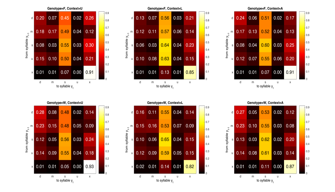
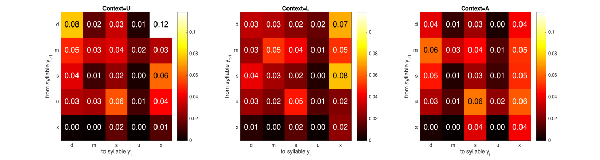
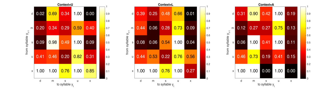
Figure 5: Results for the Foxp2 data set. Estimated posterior mean transition probabilities $P_{x_{1},x_{2}}(y_{t}\mid y_{t-1})$ for syllables $y_{t},y_{t-1}\in\{d,m,s,u,x\}$ for different combinations of genotype $x_{1}\in\{F,W\}$ and social contexts $x_{2}\in\{U,L,A\}$.

Figure 6: Results for the Foxp2 data set. The top row shows the estimated posterior mean of $\left|\Delta P_{\cdot,x_{2}}(y_{t}\mid y_{t-1})\right|=\left|P_{1,x_{2}}(y_{t}\mid y_{t-1})-P_{2,x_{2}}(y_{t}\mid y_{t-1})\right|$ for syllables $y_{t},y_{t-1}\in\{d,m,s,u,x\}$ and different social contexts $x_{2}\in\{U,L,A\}$. The bottom row shows the estimated posterior probability of $H_{0,y_{t}\mid y_{t-1},x_{2}}:\left|\Delta P_{\cdot,x_{2}}(y_{t}\mid y_{t-1})\right|\leq 0.02$.

We next focus on assessing how the absence of the Foxp2 gene influences the transition probabilities of each of the different transition types locally for each fixed context. Figure 6 summarizes the posterior mean absolute differences $\left|\Delta P_{\cdot,x_{2}}(y_{t}\mid y_{t-1})\right|$ and the posterior probabilities of the corresponding local null hypotheses $H_{0,y_{t}\mid y_{t-1},x_{2}}:\left|\Delta P_{\cdot,x_{2}}(y_{t}\mid y_{t-1})\right|\leq\delta$. For the Foxp2 experiment, $\left|\Delta P_{\cdot,x_{2}}(y_{t}\mid y_{t-1})\right|$ not exceeding $\delta=0.02$ was assumed to be practically insignificant. Results were robust to the choice of this difference threshold.

The transition types for which the corresponding local null hypotheses $H_{0,\ell}$ had estimated posterior probabilities smaller than $0.10$ were $d\to d,s\to d,d\to x,s\to x$ for context $U$; $s\to d,m\to m,s\to m,d\to x,m\to x,s\to x$ for context $F$; and $s\to d,x\to s,x\to x$ for context $A$. Comparisons between the estimated transition probabilities for the two genotypes summarized in Figure 6 suggest that, except for transitions from silence to silence in the $U$ context, the estimated transition probabilities $P_{x_{1},x_{2}}(x\mid y_{t-1})$ of moving to the special silence syllable ‘$x$’ from a preceding syllable $y_{t-1}$ are consistently larger in the Foxp2 mutant mice ($x_{1}=F$) compared to the wild type mice ($x_{1}=W$) for all $y_{t-1}\in\{d,m,s,u,x\}$ across all contexts $x_{2}\in\{U,F,A\}$. The local nulls $H_{0,\ell}$ corresponding to six of these transition types had estimated posterior probabilities less than $0.10$, and four more in the $A$ context had estimated posterior probabilities less than $0.20$. Compared to wild type mice, Foxp2 mutant mice thus had a greater tendency to transition to silence across all contexts.

The increase in the probabilities of moving to the ‘$x$’ syllable in the Foxp2 mutant mice seems to be explained by an associated decrease in the probabilities of transitioning to the ‘$d$’ syllable. Four of the associated local nulls $H_{0,\ell}$ had estimated posterior probabilities less than $0.10$, two more had estimated posterior probabilities less than $0.20$. Additionally, in the $F$ context, the estimated transition probabilities $P_{x_{1},x_{2}}(m\mid y_{t-1})$ of moving to the most complex syllable ‘$m$’ from a preceding syllable $y_{t-1}$ were smaller in the Foxp2 mutant mice compared to the wild type mice for all $y_{t-1}\in\{d,m,s,u\}$. Two of the associated local nulls $H_{0,\ell}$ were significant. Overall, these findings are consistent with the hypothesis that the Foxp2 gene plays an important role in the complexity and richness of the song dynamics, with Foxp2 knockout mice having impaired ability to produce more complex syntax.

A GLM based approach to mixed effects Markov chains, implemented via the MCMCglmm package in R (Hadfield, 2010), was also applied to the Foxp2 data set. Due to methodological limitations and computational complexities, we could only perform approximate inference with a restrictive parametric model without any interaction terms. Global significance of the exogenous predictors could not be straightforwardly assessed by such models. The approach developed in Section 4.3 to assess local differences in transition probabilities between the two genotypes could also be used for the GLM based model. However, no local difference was found to be significant. Details are deferred to Section S.3 in the Supplementary Materials.

6 Simulation Experiments

We designed simulation experiments to evaluate the performance of the proposed methodology in assessing various aspects of the vocalization dynamics in a wide range of scenarios. We tried to closely mimic many aspects of the Foxp2 data set to create scenarios typical in mouse vocalization experiments. We chose $d_{0}=5$ syllables $\{d,m,s,u,x\}$, $d_{1}=2$ genotypes $\{F,W\}$ with 8 mice from the first genotype and 6 from the other, and $d_{2}=3$ contexts $\{U,L,A\}$. The sequences were chosen to be of the same length as those in the Foxp2 data set. In each case, we set $\mbox{\boldmath$\pi$}_{0}$ and $\mbox{\boldmath$\lambda$}^{(i)}$ equal to the corresponding estimated values from the Foxp2 data set. To evaluate performance in assessing predictor effects, we considered the following scenarios:

1. $\mbox{\boldmath$\lambda$}_{x_{1},x_{2}}=\widehat{}\mbox{\boldmath$\lambda$}_{1,1}$ for $x_{1}=1,2$ and $x_{2}=1,2,3$. The vocalization dynamics vary neither with genotype nor with context ($\widetilde{k}_{10}=1$ and $\widetilde{k}_{20}=1$).

2. $\mbox{\boldmath$\lambda$}_{x_{1},x_{2}}=\widehat{}\mbox{\boldmath$\lambda$}_{x_{1},1}$ for $x_{1}=1,2$ and $x_{2}=1,2,3$. The vocalization dynamics vary with genotype but not with context ($\widetilde{k}_{10}=2$ and $\widetilde{k}_{20}=1$).

3. $\mbox{\boldmath$\lambda$}_{x_{1},x_{2}}=\widehat{}\mbox{\boldmath$\lambda$}_{1,x_{2}}$ for $x_{1}=1,2$ and $x_{2}=1,2,3$. The vocalization dynamics do not vary with genotype but vary with context ($\widetilde{k}_{10}=1$ and $\widetilde{k}_{20}=3$),

4. $\mbox{\boldmath$\lambda$}_{x_{1},x_{2}}=\widehat{}\mbox{\boldmath$\lambda$}_{x_{1},x_{2}}$ for $x_{1}=1,2$ and $x_{2}=1,2,3$. The vocalization dynamics vary with both genotype and context ($\widetilde{k}_{10}=2$ and $\widetilde{k}_{20}=3$).

5. $\mbox{\boldmath$\lambda$}_{x_{1},x_{2}}=\widehat{}\mbox{\boldmath$\lambda$}_{x_{1},x_{2}}$ for $x_{1}=1,2$ and $x_{2}=1,2$. Also, $\mbox{\boldmath$\lambda$}_{x_{1},3}=\widehat{}\mbox{\boldmath$\lambda$}_{x_{1},2}$ for $x_{1}=1,2$. The vocalization dynamics vary with both genotype and context but the dynamics within the contexts 2 and 3 are similar ($\widetilde{k}_{10}=2$ and $\widetilde{k}_{20}=2$),

6. $\mbox{\boldmath$\lambda$}_{1,x_{2}}=\widehat{}\mbox{\boldmath$\lambda$}_{1,x_{2}}$ and $\mbox{\boldmath$\lambda$}_{2,x_{2}}=\widehat{}\mbox{\boldmath$\lambda$}_{1,x_{2}}+\mbox{\boldmath$\Delta$}_{.,x_{2}}$ for $x_{2}=1,2,3$, where many cells in $\mbox{\boldmath$\Delta$}_{.,x_{2}}$ are precisely zero. The vocalization dynamics vary with both genotype and context ($\widetilde{k}_{10}=2$ and $\widetilde{k}_{20}=3$) but the differences between the dynamics for the two genotypes are strictly localized in a few specific transition types.

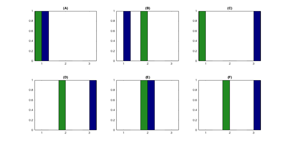
Figure 7: Results of simulation experiments. Estimated posterior probability $P(\widetilde{k}_{j}\mid{\hbox{Data}})=P(\text{the}~{}d_{j}~{}\text{levels of}~{}x_{j}~{}\text{form}~{}\widetilde{k}_{j}~{}\text{clusters}\mid{\hbox{Data}})$ for genotype $x_{1}$ in green and context $x_{2}$ in blue for different simulation scenarios discussed in Section 6.

Figure 7 shows estimated posterior probabilities $\widehat{P}(\widetilde{k}_{j}\mid{\hbox{Data}})=\widehat{P}(\widetilde{k}_{j}~{}\text{clusters in}~{}x_{ij}\mid{\hbox{Data}})$. For each simulation scenario and $j=1,2$, $\widehat{P}(\widetilde{k}_{j}=\widetilde{k}_{j0}\mid{\hbox{Data}})\approx 1$. This excellent performance in global hypothesis testing is not surprising since many small local effects can collectively produce strong evidence of overall effects.

Scenario D was closest to the Foxp2 data. Figure 9 shows estimated posterior mean transition probabilities, Figures S.2 and S.4 in the Supplementary Materials show estimated posterior standard deviations of these probabilities and the random effects parameters, respectively. Figure 9 shows estimated posterior mean absolute differences $\left|\Delta P_{\cdot,x_{2}}(y_{t}\mid y_{t-1})\right|$ and posterior probabilities of the local nulls $H_{0,y_{t}\mid y_{t-1},x_{2}}:\left|\Delta P_{\cdot,x_{2}}(y_{t}\mid y_{t-1})\right|\leq 0.02$. Comparisons with Figure 6, Figure S.2, Figure S.4 and Figure 6 show remarkable agreement between the results, suggesting high stability and reproducibility.

Scenario F was designed to evaluate the performance of the proposed method in assessing local differences between transition probabilities for the two genotypes for each fixed context. Figure 10 shows the true absolute differences $\left|\Delta P_{\cdot,x_{2}}(y_{t}\mid y_{t-1})\right|$ and the posterior probabilities of the local nulls $H_{0,y_{t}\mid y_{t-1},x_{2}}:\left|\Delta P_{\cdot,x_{2}}(y_{t}\mid y_{t-1})\right|\leq 0.02$. Out of a total of $3\times 25=75$ local tests, correct inferences were obtained in $68$ tests. There were, however, $3$ rejections of true $H_{0,\ell}$’s (false positives), and $4$ instances of failures to reject false $H_{0,\ell}$’s (false negatives).

Previously available methods for mouse song syntax analysis include Chabout et al. (2015, 2016). Using independent Markov models for each song, Chabout et al. (2015) developed chi-squared tests for assessing global differences in syntax between social contexts. Chabout et al. (2016) developed a more advanced summary statistics based approach for assessing global and local syntax differences. They first estimated the transition probabilities separately for each sequence. For comparisons between genotypes for fixed contexts, they then applied Wilcoxon-Mann-Whitney rank sum tests to these estimates. Finally, these local tests were combined using a permutation based Monte Carlo procedure to assess the global influence of genotype. Similar strategies were adopted for assessing the influences of social contexts within and across genotypes. Uncertainty in estimating the transition probabilities were, however, completely ignored. The assumption of independently distributed sequences was also highly unrealistic. More realistically, information should be shared across songs associated with same values of the exogenous predictors as well as across songs sung by the same mouse, as in our proposed formulation.

The bottom row in Figure 10 shows Benjamini-Hochberg adjusted local p-values (adjusted for 25 tests for each context) returned by the approach of Chabout et al. (2016). With a p-value threshold of $0.10$, correct inferences were obtained in $56$ of the $75$ local tests. There were $4$ rejections of true $H_{0,\ell}$’s (false positives), and $15$ failures to reject false $H_{0,\ell}$’s (false negatives). Ideally, to compare their p-value based approach with our posterior probability based procedure, we should first calibrate the p-values (Selke et al., 2001). Since, for comparable evidence levels, posterior probabilities of null hypotheses typically correspond to calibrated p-values smaller by many orders of magnitude (Berger and Selke, 1987), such calibration significantly reduces the power of these local tests, further deteriorating the results. When we used such calibration, even with our extremely liberal p-value threshold of 0.10, no $H_{0,\ell}$ was rejected.

Results for another simulated data set with similar performances are summarized in Figure S.5 in the Supplementary Materials. Comparisons with a multinomial logit based approach are also discussed in Section S.3 of the Supplementary Materials.

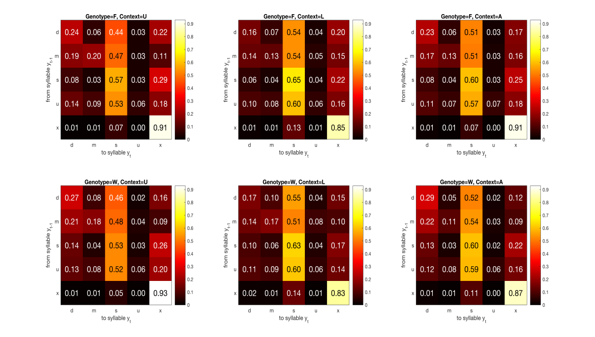
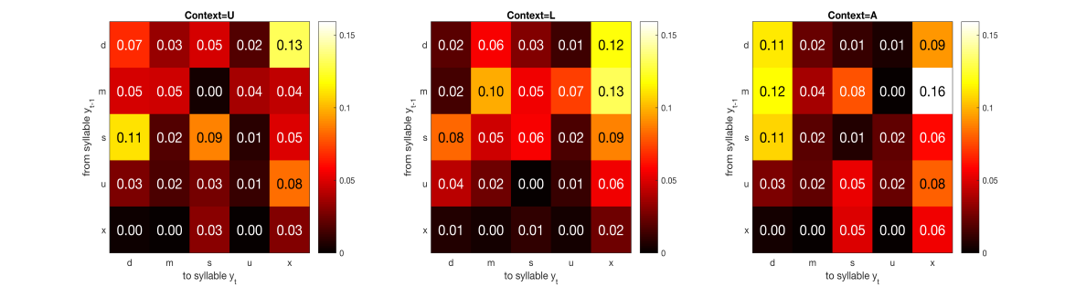
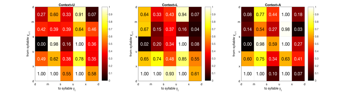
Figure 8: Results for the simulation scenario D described in Section 6. Estimated posterior mean transition probabilities $P_{x_{1},x_{2}}(y_{t}\mid y_{t-1})$ for syllables $y_{t},y_{t-1}\in\{d,m,s,u,x\}$ for different combinations of genotype $x_{1}\in\{F,W\}$ and social contexts $x_{2}\in\{U,L,A\}$.

Figure 9: Results for the simulation scenario D described in Section 6. The top row shows the estimated posterior mean of $\left|\Delta P_{\cdot,x_{2}}(y_{t}\mid y_{t-1})\right|=\left|P_{1,x_{2}}(y_{t}\mid y_{t-1})-P_{2,x_{2}}(y_{t}\mid y_{t-1})\right|$ for syllables $y_{t},y_{t-1}\in\{d,m,s,u,x\}$ and social contexts $x_{2}\in\{U,L,A\}$. The bottom row shows the estimated posterior probability of $H_{0,y_{t}\mid y_{t-1},x_{2}}:\left|\Delta P_{\cdot,x_{2}}(y_{t}\mid y_{t-1})\right|\leq 0.02$.

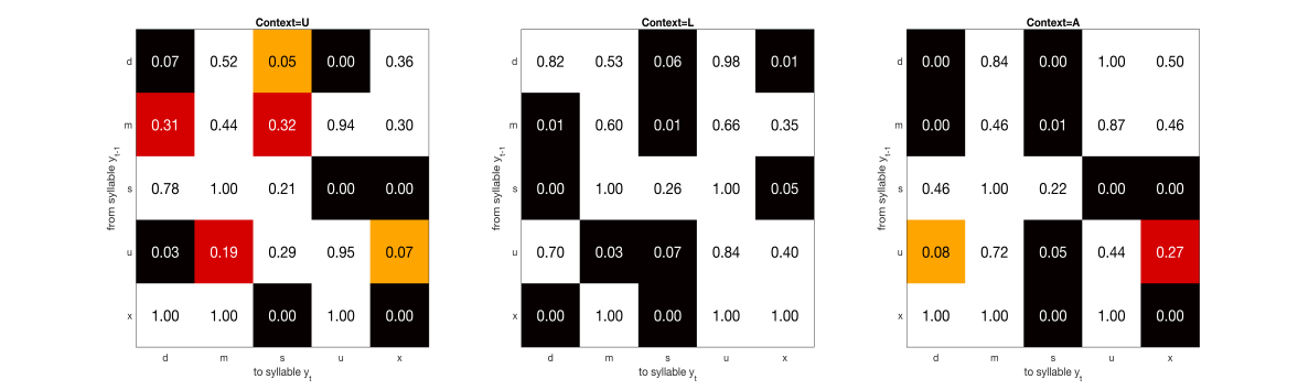
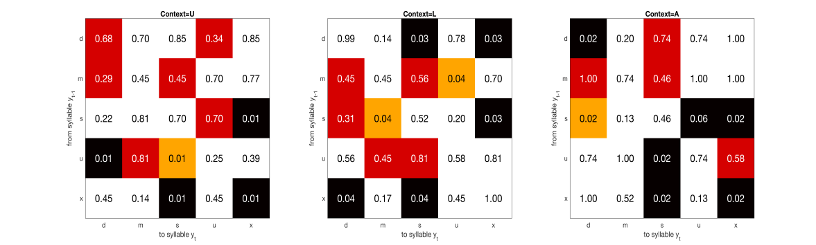
Figure 10: Results for the simulation scenario F described in Section 6. The top row shows the true values of $\left|\Delta P_{\cdot,x_{2}}(y_{t}\mid y_{t-1})\right|=\left|P_{1,x_{2}}(y_{t}\mid y_{t-1})-P_{2,x_{2}}(y_{t}\mid y_{t-1})\right|$ for syllables $y_{t},y_{t-1}\in\{d,m,s,u,x\}$ and social contexts $x_{2}\in\{U,L,A\}$. Positive differences are highlighted in black. The middle row shows the estimated posterior probabilities of $H_{0,y_{t}\mid y_{t-1},x_{2}}:\left|\Delta P_{\cdot,x_{2}}(y_{t}\mid y_{t-1})\right|\leq 0.02$. The bottom row shows Benjamini-Hochberg adjusted p-values obtained using the method of Chabout et al. (2016). Posterior probabilities smaller than $0.1$ are considered significant and are highlighted in black and orange. Posterior probabilities greater than $0.1$ are presented in white and red. Likewise, p-values smaller than $0.1$ are considered significant and are highlighted in black and orange. P-values greater than $0.1$ are presented in white and red. White and black cells represent correct decisions, orange cells mark rejections of true $H_{0,\ell}$ (false positives), and red cells mark failures to reject false $H_{0,\ell}$ (false negatives).

7 Discussion

This article introduced a flexible, computationally efficient mixed effects Markov model, providing a sophisticated framework for inference in mouse vocalization experiments. While the focus was on a particular study assessing the effects of a Foxp2 mutation, the methodology is applicable generally to other vocalization experiments having similar data structures and should have significant impact in such settings. As it is sometimes of interest to assess changes during development (Castellucci et al., 2016; Scattoni et al., 2008a), it will be important in ongoing research to generalize the model to allow dynamic changes with age. Although our motivation here was mouse vocalization experiments, the methods have potential far beyond such applications. Natural extensions, which are conceptually straightforward, include accommodation of hidden Markov Models, continuous predictors, and time-varying predictors.

Supplementary Materials

Supplementary Materials present theoretical properties, and additional figures summarizing the results for the real and the simulated data sets described in Section 5 and Section 6. Supplementary Materials also present additional comparisons of the proposed approach with generalized linear mixed model based approaches.

Supplementary Materials for
Bayesian Semiparametric Mixed Effects Markov Chains

The Supplementary Materials discuss some theoretical aspects of our model; present additional figures summarizing the results for the real and the simulated data sets described in Section 5 and Section 6 in the main paper; and discuss the contrasting features of generalized linear mixed model based approaches with our proposed approach, highlighting the latter’s many advantages over the former.

S.1 Theoretical Properties

In this section, we discuss some theoretical aspects of our proposed model. We follow the notations and definitions of the main paper.

For Markov chains with exogenous predictors (MCEPs), the values of the exogenous predictors remain fixed for the entire lengths of the sequences. The notions of ergodicity, stationarity etc for predictor free ordinary Markov chains thus extend naturally to MCEPs. Let ${\cal P}_{0}=\{P_{0,x_{1},\dots,x_{p}}^{(i)}(y_{t}\mid y_{t-1}):P_{0,x_{1},\dots,x_{p}}^{(i)}(y_{t}\mid y_{t-1})=\pi_{0,0}(y_{t-1})\mbox{\boldmath$\lambda$}_{0,x_{1},\dots,x_{p}}(y_{t}\mid y_{t-1})+\pi_{0,1}(y_{t-1})\mbox{\boldmath$\lambda$}_{0}^{(i)}(y_{t}\mid y_{t-1})\}\subset{\cal P}$ denote the class of transition probability distributions that admit representations similar to our proposed formulation. It is straightforward to check that any ${\mathbf{P}}_{0,x_{1},\dots,x_{p}}^{(i)}(\cdot\mid y_{t-1})\in{\cal P}_{0}$ will be ergodic if at least one of the component transition distributions is also so and the associated mixture probability is strictly positive. In particular, if $\mbox{\boldmath$\lambda$}_{0,x_{1},\dots,x_{p}}(\cdot\mid y_{t-1})$ and $\mbox{\boldmath$\lambda$}_{0}^{(i)}(\cdot\mid y_{t-1})$ are both ergodic with stationary distributions $\mbox{\boldmath$\pi$}_{0,x_{1},\dots,x_{p}}=\{\pi_{0,x_{1},\dots,x_{p}}(1),\dots,\pi_{0,x_{1},\dots,x_{p}}(d_{0})\}^{\rm T}$ and $\mbox{\boldmath$\pi$}_{0}^{(i)}=\{\pi_{0}^{(i)}(1),\dots,\pi_{0}^{(i)}(d_{0})\}^{\rm T}$, respectively, then the stationary distribution of ${\mathbf{P}}_{0,x_{1},\dots,x_{p}}^{(i)}(\cdot\mid y_{t-1})$, denoted by $\mbox{\boldmath$\pi$}_{0,x_{1},\dots,x_{p}}^{(i)}=\{\pi_{0,x_{1},\dots,x_{p}}^{(i)}(1),\dots,\pi_{0,x_{1},\dots,x_{p}}^{(i)}(d_{0})\}^{\rm T}$, has a representation $\pi_{0,x_{1},\dots,x_{p}}^{(i)}(y_{t})=\pi_{0}(y_{t})\pi_{0,x_{1},\dots,x_{p}}(y_{t})+\pi_{1}(y_{t})\pi_{0}^{(i)}(y_{t})$. Conversely, if $\pi_{0}(y_{t-1})\in(0,1)$, ${\mathbf{P}}_{0,x_{1},\dots,x_{p}}^{(i)}(\cdot\mid y_{t-1})$ can be ergodic even when neither of the two component distributions are so. This can be seen by constructing an example with binary state space $\{1,2\}$ where one of the component transition distributions only allows self transitions ($1\to 1,2\to 2$) and the other only transitions to the other state ($1\to 2,2\to 1$). These results all follow from basic definitions of stationarity and also extend naturally to population level transition distributions ${\mathbf{P}}_{0,x_{1},\dots,x_{p}}(\cdot\mid y_{t-1})$.

We now discuss model flexibility, prior support and posterior consistency. The proposed mixed effect Markov model assumes additivity of predictor effects and individual effects directly on the probability scale. The model assumes an implicit upper bound $\pi_{1}(y_{t-1})$ on how far the individual effects $\pi_{1}(y_{t-1})\mbox{\boldmath$\lambda$}^{(i)}(y_{t}\mid y_{t-1})$ can stretch the effects due to the exogenous predictors $\pi_{0}(y_{t-1})\mbox{\boldmath$\lambda$}_{h_{1},\dots,h_{p}}(y_{t}\mid y_{t-1})$ in modeling ${\mathbf{P}}_{h_{1},\dots,h_{p}}^{(i)}(y_{t}\mid y_{t-1})$. This bound can be easily relaxed by allowing the $\pi_{1}(y_{t-1})$’s to also be individual specific with a multi-level hierarchical prior on them. We have not pursued such generalizations in this article in favor of simplicity and parsimony. Being based on the partition model for MCEPs introduced in Section 3.1 in the main paper, the model for the population level mean transition probabilities ${\mathbf{P}}_{h_{1},\dots,h_{p}}(\cdot\mid y_{t-1})$, on the other hand, is fully nonparametric, taking into account all order interactions between the exogenous and the local predictors. The class ${\cal P}_{0}$, defined above, thus denotes a fairly large class of individual specific exogenous predictor dependent transition distributions.

It is easy to check that our assumed priors, referred to collectively as $\Pi$, assign positive probability on any arbitrarily close $L_{1}$ neighborhood of any ${\mathbf{P}}_{0}=\{P_{0,x_{s,1},\dots,x_{s,p}}^{(i_{s})}(y_{t}\mid y_{t-1})\}_{s=1}^{s_{0}}\in{\cal P}_{0}$. More formally, with $d(P_{x_{1},\dots,x_{p}}^{(i)},P_{0,x_{1},\dots,x_{p}}^{(i)})=\sum_{y_{t-1}=1}^{d_{0}}\sum_{y_{t}=1}^{d_{0}}\left|P_{x_{1},\dots,x_{p}}^{(i)}(y_{t}\mid y_{t-1})-P_{0,x_{1},\dots,x_{p}}^{(i)}(y_{t}\mid y_{t-1})\right|$, we have $\Pi\{{\cal B}_{\delta}({\mathbf{P}}_{0})\}>0$ for any ${\mathbf{P}}_{0}\in{\cal P}_{0}$ and any $\delta>0$, where ${\cal B}_{\delta}({\mathbf{P}}_{0})=\{P_{x_{s,1},\dots,x_{s,p}}^{(i_{s})}:d(P_{x_{s,1},\dots,x_{s,p}}^{(i_{s})},P_{0,x_{s,1},\dots,x_{s,p}}^{(i_{s})})\leq\delta,s=1,\dots,s_{0}\}$.

Let ${\cal P}_{00}\subset{\cal P}_{0}$ be the class of ergodic transition probability distributions ${\mathbf{P}}_{0}$ with associated stationary distributions $\pi^{(i)}_{0,x_{1},\dots,x_{p}}(y_{t})$, where $\pi^{(i)}_{0,x_{1},\dots,x_{p}}(y_{t})>0$ for all $y_{t}\in{\cal S}_{0}$. Assuming $\{y_{s,t}\}_{s=1,t=1}^{s_{0},T_{s}}$ to be ergodic with the true transition dynamics characterized by some ${\mathbf{P}}_{0}\in{\cal P}_{00}$, it then follows, using strong law of large numbers for ergodic Markov chains (Eichelsbacher and Ganesh, 2002), that the posterior $\Pi[\cdot\mid\{x_{s,j},y_{s,t}\}_{s=1,t=1,j=1}^{s_{0},T_{s},p}]$ concentrates almost surely in arbitrarily small neighborhoods of the true data generating parameters ${\mathbf{P}}_{0}$ as $\min_{s}T_{s}\to\infty$ (Ghosh and Ramamoorthi, 2003). Formally, for any $\delta>0$ and any ${\mathbf{P}}_{0}\in{\cal P}_{00}$, $\Pi[{\cal B}_{\delta}({\mathbf{P}}_{0})\mid\{x_{s,j},y_{s,t}\}_{s=1,t=1,j=1}^{s_{0},T_{s},p}]\to 1~{}\text{almost surely}~{}{\mathbf{P}}_{0}~{}\text{as}~{}\min_{s}T_{s}\to\infty$.

Asymptotic regimes for classical mixed effects models typically assume the number of subjects to approach infinity while the number of observations for each subject remains fixed. The criteria considered here, on the contrary, assumes the number of subjects to remain fixed but assumes the length of each sequence to approach infinity. This is a more realistic scenario for animal vocalization experiments, since it is practically impossible to study more than a small to moderate number of mice from each genotype. The recording times of the songs, however, can be easily increased.

S.2 Additional Figures

This section presents additional figures summarizing the analyses of the Foxp2 data set and the simulation experiments, described in Sections 5 and 6 in the main paper, respectively.

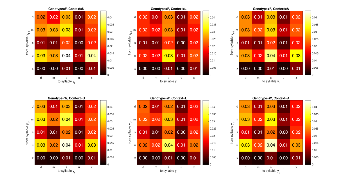
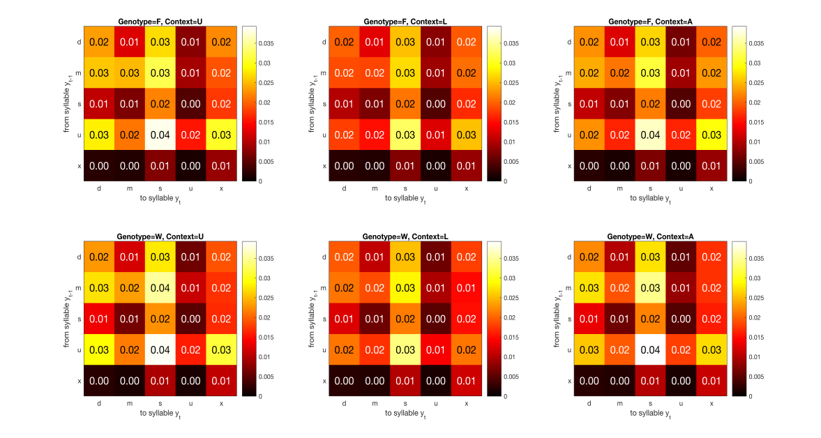
Figure S.1: Results for the Foxp2 data set. Estimated posterior standard deviation of transition probabilities $P_{x_{1},x_{2}}(y_{t}\mid y_{t-1})$ for syllables $y_{t},y_{t-1}\in\{d,m,s,u,x\}$ for different combinations of genotype $x_{1}\in\{F,W\}$ and social contexts $x_{2}\in\{U,L,A\}$.

Figure S.2: Results for the simulation scenario D described in Section 6 of the main paper. Estimated posterior standard deviation of transition probabilities $P_{x_{1},x_{2}}(y_{t}\mid y_{t-1})$ for syllables $y_{t},y_{t-1}\in\{d,m,s,u,x\}$ for different combinations of genotype $x_{1}\in\{F,W\}$ and social contexts $x_{2}\in\{U,L,A\}$.

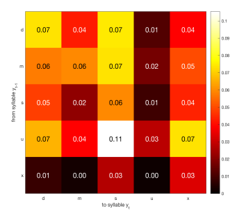
Figure S.3: Results for the Foxp2 data set. Estimated posterior standard deviation of the random effects parameters $\pi_{1}(y_{t-1})\lambda^{(i)}(y_{t}\mid y_{t-1})$ for syllables $y_{t},y_{t-1}\in\{d,m,s,u,x\}$.

Figure S.4: Results for the simulation scenario D described in Section 6 of the main paper. Estimated posterior standard deviation of the random effects parameters $\pi_{1}(y_{t-1})\lambda^{(i)}(y_{t}\mid y_{t-1})$ for syllables $y_{t},y_{t-1}\in\{d,m,s,u,x\}$.

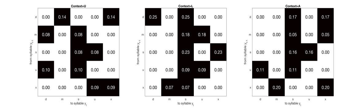
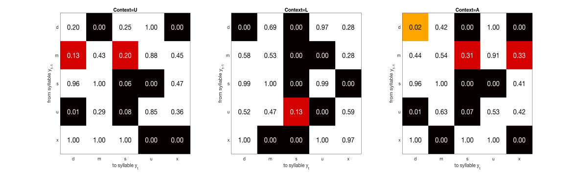
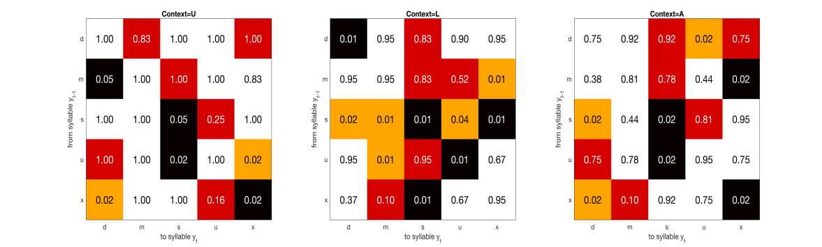
Figure S.5: Results for the simulation scenario F described in Section 6 in the main paper, but for a different random seed. The top row shows the true values of $\left|\Delta P_{\cdot,x_{2}}(y_{t}\mid y_{t-1})\right|=\left|P_{1,x_{2}}(y_{t}\mid y_{t-1})-P_{2,x_{2}}(y_{t}\mid y_{t-1})\right|$ for syllables $y_{t},y_{t-1}\in\{d,m,s,u,x\}$ and social contexts $x_{2}\in\{U,L,A\}$. Positive differences are highlighted in black. The middle row shows the estimated posterior probabilities of $H_{0,y_{t}\mid y_{t-1},x_{2}}:\left|\Delta P_{\cdot,x_{2}}(y_{t}\mid y_{t-1})\right|\leq 0.02$. The bottom row shows Benjamini-Hochberg adjusted p-values obtained using the method of Chabout et al. (2016). Posterior probabilities smaller than $0.1$ are considered significant and are highlighted in black and orange. Posterior probabilities greater than $0.1$ are presented in white and red. Likewise, p-values smaller than $0.1$ are considered significant and are highlighted in black and orange. P-values greater than $0.1$ are presented in white and red. White and black cells represent correct decisions, orange cells mark rejections of true $H_{0,\ell}$ (false positives), and red cells mark failures to reject false $H_{0,\ell}$ (false negatives).

S.3 Comparison with GLM Based Approach

In this section, we revisit GLM based approaches to mixed effects Markov chains. Adapting to Altman (2007), without any interaction among the local predictor $y_{t-1}$ and the exogenous predictors $x_{j},j=1,\dots,p$, using the logit link, we are now required to formulate $d_{0}-1$ models, one for each $y_{t}=1,\dots,d_{0}-1$, of the form

$$\hbox{log}\left\{\frac{P_{x_{s,1},\dots,x_{s,p}}^{(i_{s})}(y_{s,t}\mid y_{s,t-1})}{P_{x_{s,1},\dots,x_{s,p}}^{(i_{s})}(d_{0}\mid y_{s,t-1})}\right\}=$$

$$~{}~{}\beta_{0,y_{t}}+\sum_{y_{t-1}=1}^{d_{0}-1}\beta_{y_{t},y_{t-1}}1\{y_{s,t-1}=y_{t-1}\}+\sum_{j=1}^{p}\sum_{x_{j}=1}^{d_{j}-1}\beta_{j,y_{t},x_{j}}1\{x_{s,j}=x_{j}\}+u_{y_{t},y_{t-1}}^{(i_{s})},$$

where ${\mathbf{u}}^{(i)}=\{u_{y_{t},y_{t-1}}^{(i)}\}_{y_{t}=1,y_{t-1}=1}^{d_{0}-1,d_{0}}$ are random effects to due to the $i^{th}$ individual. Except for the restrictive special case of binary sequences, estimation of the model parameters becomes prohibitively complex, especially in presence of multiple exogenous predictors. Incorporating only second order interactions would require an additional $N_{int}=\sum_{j_{1}=0}^{p}\sum_{j_{2}=0,j_{1}\neq j_{2}}^{p}(d_{j_{1}}-1)(d_{j_{2}}-1)$ terms for each of the $d_{0}-1$ models, significantly increasing model complexities. For the Foxp2 application, for instance, this would require $N_{int}=14$ additional terms in each of the $4$ models. We have thus ignored interactions among the exogenous and the local predictors here.

The population average probabilities implied by the model can be obtained by integrating out the random effects as

$$P_{x_{1},\dots,x_{p}}(y_{t}\mid y_{t-1})=\int P_{x_{1},\dots,x_{p}}^{(i)}(y_{t}\mid y_{t-1})f({\mathbf{u}}_{y_{t-1}}^{(i)})d{\mathbf{u}}_{y_{t-1}}^{(i)}=$$

$$~{}~{}\int\frac{\exp\left(\beta_{0,y_{t}}+\beta_{y_{t},y_{t-1}}+\sum_{j=1}^{p}\beta_{j,y_{t},x_{j}}+u_{y_{t},y_{t-1}}^{(i)}\right)}{\sum_{h=1}^{d_{0}}\exp\left(\beta_{0,h}+\beta_{h,y_{t-1}}+\sum_{j=1}^{p}\beta_{j,h,x_{j}}+u_{h,y_{t-1}}^{(i)}\right)}f({\mathbf{u}}_{y_{t-1}}^{(i)})d{\mathbf{u}}_{y_{t-1}}^{(i)},$$

where $\beta_{0,d_{0}}=0$, $\beta_{d_{0},y_{t-1}}=\beta_{1,d_{0},y_{t-1}}=\dots=\beta_{p,d_{0},y_{t-1}}=u_{d_{0},y_{t-1}}^{(i)}=0$ for all $y_{t-1}$, ${\mathbf{u}}_{y_{t-1}}^{(i)}=(u_{1,y_{t-1}}^{(i)},\dots,u_{d_{0}-1,y_{t-1}}^{(i)})^{\rm T}$, and $f({\mathbf{u}}_{y_{t-1}}^{(i)})$ is the random effects distribution. Typically it is assumed that $f({\mathbf{u}}_{y_{t-1}}^{(i)})=\hbox{MVN}_{d_{0}-1}({\mathbf{0}},\mbox{\boldmath$\Sigma$}_{u})$, where $\hbox{MVN}_{q}(\mbox{\boldmath$\mu$},\mbox{\boldmath$\Sigma$})$ denotes a $q$-dimensional multivariate normal distribution with mean vector $\mu$ and covariance matrix $\Sigma$. Often such models are further simplified by assuming ${\mathbf{u}}_{y_{t-1}}^{(i)}={\mathbf{u}}^{(i)}$ for all $y_{t-1}$ (Altman, 2007) and the components of ${\mathbf{u}}_{y_{t}}$ to be distributed independently with $\mbox{\boldmath$\Sigma$}_{u}=\hbox{diag}(\sigma_{u,1}^{2},\dots,\sigma_{u,d_{0}-1}^{2})$.

Even with such restrictive simplifying assumptions, the population level transition probabilities $P_{x_{1},\dots,x_{p}}(y_{t}\mid y_{t-1})$ do not have closed form expressions. Assuming $P_{x_{1},\dots,x_{p}}(y_{t}\mid y_{t-1})$ to arise from the same multinomial logit functional form

$$P_{x_{1},\dots,x_{p}}(y_{t}\mid y_{t-1})=\frac{\exp\left(\beta_{0,y_{t}}^{\star}+\beta_{y_{t},y_{t-1}}^{\star}+\sum_{j=1}^{p}\beta_{j,y_{t},x_{j}}^{\star}\right)}{\sum_{h=1}^{d_{0}}\exp\left(\beta_{0,h}^{\star}+\beta_{h,y_{t-1}}^{\star}+\sum_{j=1}^{p}\beta_{j,h,x_{j}}^{\star}\right)},$$

an approximation yields $\beta_{0,y_{t}}^{\star}\approx\beta_{0,y_{t}}/(1+c^{2}\sigma_{u,y_{t}}^{2})^{1/2},\beta_{y_{t},y_{t-1}}^{\star}\approx\beta_{y_{t},y_{t-1}}/(1+c^{2}\sigma_{u,y_{t}}^{2})^{1/2}$ and so on, where $c=(16\sqrt{3})/(15\pi)$ (Zeger et al., 1988). Individual and population level fixed effects parameters are thus different and have to be differently interpreted. Specifically, population level probabilities depend on individual heterogeneity - two populations with different individual heterogeneity will have different population level probabilities even if they have the same individual level fixed effects parameters.

Testing scientific hypotheses related to influences of the predictors using such GLM based models is also complicated. For instance, the global null $H_{0j}$ of no effect of the $j^{th}$ exogenous predictor $x_{j}$, when translated in terms of the model parameters, becomes a complicated composite hypothesis $H_{0j}:\beta_{j,y_{t},x_{j}}=0$ for all $y_{t}=1,\dots,d_{0}-1$ and all $x_{j}=1,\dots,d_{j}-1$.

In comparison, our model is highly flexible, parsimoniously accommodating interactions of all orders between the exogenous and the local predictors. The random effects in our model for the individual level transition probabilities can be easily integrated out to obtain closed form expressions of the population level transition probabilities. The fixed effects components remain the same in both individual and population level probabilities and hence can be interpreted in the same way. Finally, testing scientific hypotheses related to global influences of the predictors is very straightforward using our approach as they can be translated in terms of a single model parameter.

We implemented the multinomial logit based mixed effects Markov model described above using the MCMCglmm package in R (Hadfield, 2010). Maximum likelihood estimation of the model parameters using other R packages did not produce realistic results. Figure S.7 shows the estimated posterior means of the population level transition probabilities based on $12,000$ samples drawn from the posterior, thinned by an interval of $10$ after the initial $2,000$ were discarded as burnin. Comparison with estimates produced by our method, summarized in Figure 6 in the main paper, suggests overall agreement. For reasons detailed above, global significance of the exogenous predictors could not be straightforwardly assessed. We could, however, assess the significance of each $\beta$ parameter from the MCMC output using the minimum of the proportion of samples in which $\beta$ is on one side or the other of zero, referred to as pMCMC in MCMCglmm. For the Foxp2 data set, the four $\beta$ parameters associated with genotype, namely $\beta_{1,1,1},\beta_{1,2,1},\beta_{1,3,1},\beta_{1,4,1}$, had pMCMC values $0.446$, $0.436$, $0.368$ and $0.106$, indicating none of them to be marginally significant. To assess local differences in transition probabilities between the two genotypes, we employed the approach developed in Section 4.3 of the main paper. Figure S.7 summarizes the posterior probabilities of the local null hypotheses $H_{0,y_{t}\mid y_{t-1},x_{2}}:\left|\Delta P_{\cdot,x_{2}}(y_{t}\mid y_{t-1})\right|\leq 0.02$ estimated from the MCMC output of the GLM based model. Unlike the results produced by our approach, summarized in Figure 6 in the main paper, no local difference was found to be significant at the $0.10$ posterior probability level.

To further assess how the multinomial logit based mixed effects Markov model compares with our proposed approach in detecting local differences in transition probabilities between the two genotypes, we compared the results produced by the two methods for data sets simulated under scenario F described in Section 6 in the main paper. The posterior means of the population level transition probabilities estimated by the GLM based approach (not shown here) were quite different from the truth. Figures S.8 and S.9 summarize the estimated posterior probabilities of the local null hypotheses $H_{0,y_{t}\mid y_{t-1},x_{2}}:\left|\Delta P_{\cdot,x_{2}}(y_{t}\mid y_{t-1})\right|\leq 0.02$ for two different simulated data sets. Compared to the results produced by our approach, summarized in Figure 10 and Figure S.5, there were many more false decisions.

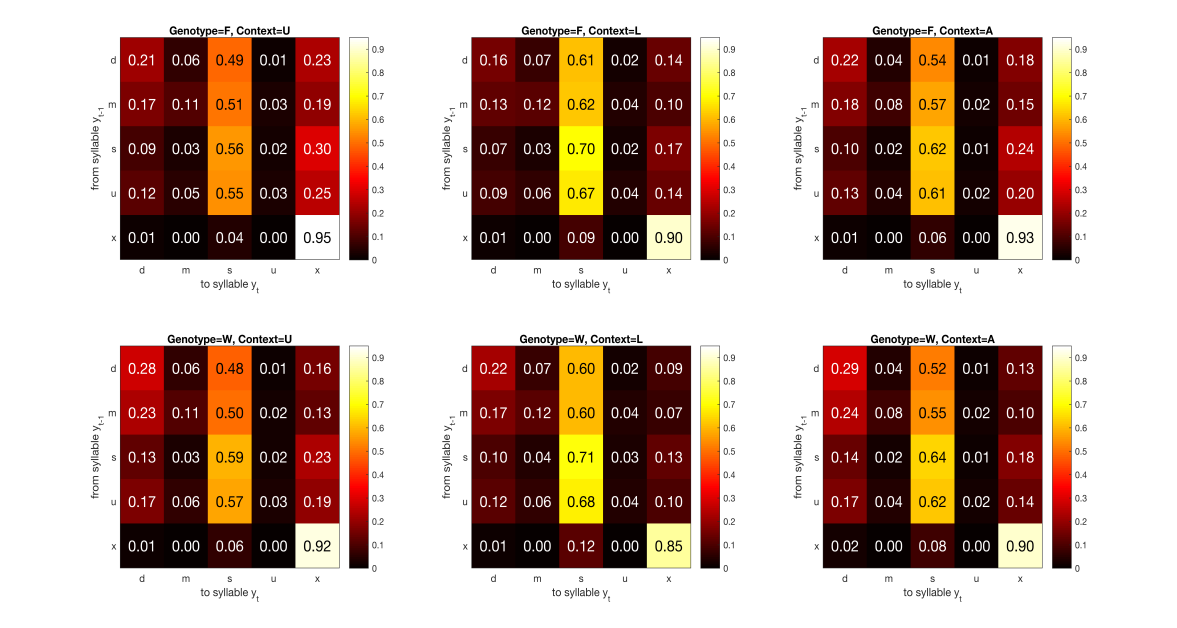
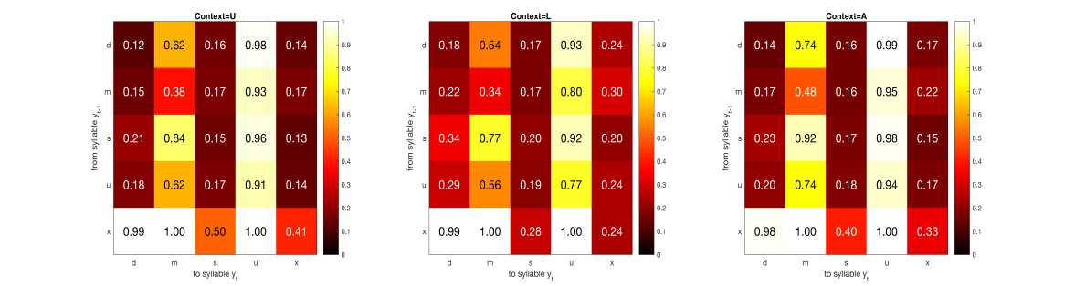
Figure S.6: Results for the Foxp2 data set for the GLM based approach described in Section S.3 in the Supplementary Materials. Estimated approximate posterior mean transition probabilities $P_{x_{1},x_{2}}(y_{t}\mid y_{t-1})$ for syllables $y_{t},y_{t-1}\in\{d,m,s,u,x\}$ for different combinations of genotype $x_{1}\in\{F,W\}$ and social contexts $x_{2}\in\{U,L,A\}$.

Figure S.7: Results for the Foxp2 data set for the GLM based approach described in Section S.3 in the Supplementary Materials. The estimated posterior probability of $H_{0,y_{t}\mid y_{t-1},x_{2}}:\left|\Delta P_{\cdot,x_{2}}(y_{t}\mid y_{t-1})\right|=\left|P_{1,x_{2}}(y_{t}\mid y_{t-1})-P_{2,x_{2}}(y_{t}\mid y_{t-1})\right|\leq 0.02$.

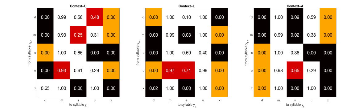
Figure S.8: Results for the simulation scenario F described in Section 6 in the main paper. These results were produced by the GLM based approach described in Section S.3 in the Supplementary Materials. The results show the estimated posterior probabilities of $H_{0,y_{t}\mid y_{t-1},x_{2}}:\left|\Delta P_{\cdot,x_{2}}(y_{t}\mid y_{t-1})\right|\leq 0.02$. Posterior probabilities smaller than $0.1$ are considered significant and are highlighted in black and orange. Posterior probabilities greater than $0.1$ are presented in white and red. White and black cells represent correct decisions, orange cells mark rejections of true $H_{0,\ell}$ (false positives), and red cells mark failures to reject false $H_{0,\ell}$ (false negatives). Compare with Figure 10 in the main paper.

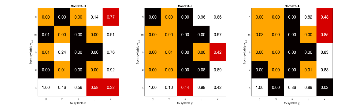
Figure S.9: Results for the simulation scenario F described in Section 6 in the main paper, but for a different random seed. These results were produced by the GLM based approach described in Section S.3 in the Supplementary Materials. The results show the estimated posterior probabilities of $H_{0,y_{t}\mid y_{t-1},x_{2}}:\left|\Delta P_{\cdot,x_{2}}(y_{t}\mid y_{t-1})\right|\leq 0.02$. Posterior probabilities smaller than $0.1$ are considered significant and are highlighted in black and orange. Posterior probabilities greater than $0.1$ are presented in white and red. White and black cells represent correct decisions, orange cells mark rejections of true $H_{0,\ell}$ (false positives), and red cells mark failures to reject false $H_{0,\ell}$ (false negatives). Compare with Figure S.5 in the Supplementary Materials.

References

Altman, R. M. (2007). Mixed hidden Markov models: an extension of the hidden Markov model to the longitudinal data setting. Journal of the American Statistical Association, 102, 201-210.

Eichelsbacher, P. and Ganesh, A. (2002). Bayesian inference for Markov chains. Journal of Applied Probability, 39, 91-99.

Ghosh, J. K. and Ramamoorthi, R. V. (2003). Bayesian nonparametrics. Springer Verlag, Berlin.

Hadfield, J. D. (2010). MCMC methods for multi-response generalized linear mixed models: The MCMCglmm R package. Journal of Statistical Software, 33, 1-22.

Zeger, S. L., Liang, K.-Y., and Albert, P. S. (1988). Models for longitudinal data: a generalized estimating equation approach. Biometrics, 44, 1049-1060.

References

- Agresti (2013) Agresti, A. (2013). Categorical data analysis. John Wiley & Sons, Hoboken, New Jersey, Third edition.
- Altman (2007) Altman, R. M. (2007). Mixed hidden Markov models: an extension of the hidden Markov model to the longitudinal data setting. Journal of the American Statistical Association, 102, 201–210.
- Arriaga et al. (2012) Arriaga, G., Zhou, E. P., and Jarvis, E. D. (2012). Of mice, birds, and men: the mouse ultrasonic song system has some features similar to humans and song-learning birds. PLoS ONE, 7:e46610. doi: 10.1371/journal.pone.0046610.
- Azzalini (1994) Azzalini, A. (1994). Logistic regression for autocorrelated data with application to repeated measures. Biometrika, 81, 767–775.
- Berger and Selke (1987) Berger, J. O. and Selke, T. (1987). Testing a point null hypothesis: The irreconcilability of p values and evidence. Journal of the American Statistical Association, 82, 112–122.
- Bizzotto et al. (2010) Bizzotto, R., Zamuner, S., De Nicolao, G., Karlsson, M. O., and Gomeni, R. (2010). Multinomial logistic estimation of Markov-chain models for modeling sleep architecture in primary insomnia patients. Journal of Pharmacokinetics and Pharmacodynamics, 37, 137–155.
- Bonney (1987) Bonney, G. E. (1987). Logistic regression for dependent binary observations. Biometrics, 43, 951–973.
- Breiman et al. (1984) Breiman, L., Friedman, J., Olshen, R., and Stone, C. (1984). Classification and Regression Trees. Wadsworth.
- Castellucci et al. (2016) Castellucci, G. A., McGinley, M. J., and McCormick, D. A. (2016). Knockout of Foxp2 disrupts vocal development in mice. Nature Scientific Reports, 6. doi: 10.1038/srep23305.
- Chabout et al. (2012) Chabout, J., Serreau, P., Ey, E., Bellier, L., Aubin, T., Bourgeron, T., and Granon, S. (2012). Adult male mice emit context-specific ultrasonic vocalizations that are modulated by prior isolation or group rearing environment. PLoS ONE, 7:e29401. doi: 10.1371/journal.pone.0046610.
- Chabout et al. (2015) Chabout, J., Sarkar, A., Dunson, D. B., and Jarvis, E. D. (2015). Male song syntax depends on contexts and influences female preferences in mice. Frontiers in Behavioral Neuroscience, 9, 1–19.
- Chabout et al. (2016) Chabout, J., Sarkar, A., Patel, S., Raiden, T., Dunson, D. B., Fisher, S. E., and Jarvis, E. D. (2016). A Foxp2 mutation implicated in human speech deficits alters sequencing of ultrasonic vocalizations in adult male mice. Frontiers in Behavioral Neuroscience, 10, 1–18.
- Delattre (2010) Delattre, M. (2010). Inference in mixed hidden Markov models and applications to medical studies. Journal de la Société française de statistique, 151, 90–105.
- Denison et al. (1998) Denison, D. G. T., Mallick, B. K., and Smith, A. F. M. (1998). A Bayesian CART algorithm. Biometrika, 85, 363–377.
- Dunson (2006) Dunson, D. B. (2006). Bayesian dynamic modeling of latent trait distributions. Biostatistics, 7, 551–568.
- Fitzmaurice and Liard (1993) Fitzmaurice, M. G. and Liard, N. M. (1993). A likelihood-based method for analysing longitudinal binary responses. Biometrika, 80, 141–151.
- Fujita et al. (2008) Fujita, E., Tanabe, Y., Shiota, A., Ueda, M., Suwa, K., Momoi, M. Y., and Momoi, T. (2008). Ultrasonic vocalization impairment of Foxp2 (R552H) knockin mice related to speech-language disorder and abnormality of Purkinje cells. Proceedings of the National Academy of Sciences, 105, 3117–3122.
- Gaub et al. (2016) Gaub, S., Fisher, S. E., and Ehret, G. (2016). Ultrasonic vocalizations of adult male Foxp2 mutant mice: behavioral contexts of arousal and emotion. Genes, Brain and Behavior, 15, 243–259.
- Hadfield (2010) Hadfield, J. D. (2010). MCMC methods for multi-response generalized linear mixed models: The MCMCglmm R package. Journal of Statistical Software, 33, 1–22.
- Haesler et al. (2004) Haesler, S., Wada, K., Nshdejan, A., Morrisey, E. E., Lints, T., Jarvis, E. D., and Scharff, C. (2004). FoxP2 expression in avian vocal learners and non-learners. Journal of Neuroscience, 24, 3164–3175.
- Holy and Guo (2005) Holy, T. E. and Guo, Z. (2005). Ultrasonic songs of male mice. PLoS Biology, 3, 2177–2186.
- Hudges and Guttorp (1994) Hudges, J. P. and Guttorp, P. (1994). A class of stochastic models for relating synoptic atmospheric patterns to regional hydrologic phenomena. Water Resources Research, 30, 1535–1546.
- Islam et al. (2013) Islam, M. A., Chowdhury, R. I., and Huda, S. (2013). A multistate transition model for analyzing longitudinal depression data. Bulletin of the Malaysian Mathematical Sciences Society, 36, 637–655.
- Kaas (2006) Kaas, J. H., editor (2006). Evolution of Nervous Systems. Elsevier, San Diego.
- Lai et al. (2003) Lai, J., Gerrelli, D., Monaco, A. P., Fisher, S. E., and Copp, A. J. (2003). FOXP2 expression during brain development coincides with adult sites of pathology in a severe speech and language disorder. Brain, 126, 2455–2462.
- Law et al. (2000) Law, J., Boyle, J., Harris, F., Avril Harkness, A., and Nye, C. (2000). Prevalence and natural history of primary speech and language delay: findings from a systematic review of the literature. International Journal of Language and Communication Disorders, 35, 165–188.
- Marler and Slabbekoorn (2004) Marler, P. R. and Slabbekoorn, H., editors (2004). Nature’s Music: The Science of Birdsong. Elsevier, San Diego.
- Maruotti (2011) Maruotti, A. (2011). Mixed hidden Markov models for longitudinal data: an overview. International Statistical Review, 79, 427–454.
- Maruotti and Rydén (2009) Maruotti, A. and Rydén, T. (2009). A semiparametric approach to hidden Markov models under longitudinal observations. Statistics and Computing, 19, 381–393.
- McCullagh and Nelder (1989) McCullagh, P. and Nelder, J. A. (1989). Generalizaed Linear Models. Chapman & Hall, London and New York, Second edition.
- Müller et al. (2004) Müller, P., Quintana, F., and Rosner, G. (2004). A method for combining inference across related nonparametric Bayesian models. Journal of the Royal Statistical Society, Series B, 66, 735–749.
- Musolf et al. (2015) Musolf, K., Meindl, S., Larsen, A. L., Kalcounis-Rueppell, M. C., and J., P. D. (2015). Ultrasonic vocalizations of male mice differ among species and females show assortative preferences for male calls. PLoS ONE, 10:e0134123. doi:10.1371/journal.pone.0134123.
- NIH-NIDCD Report (2010) NIH-NIDCD Report (2010). Statistics about voice, speech, language, and swallowing. http://www.nidcd.nih.gov/health/statistics/vsl/Pages/stats.aspx.
- Rahman and Islam (2007) Rahman, M. S. and Islam, M. A. (2007). Markov structure based logistic regression for repeated measures: An application to diabetes mellitus data. Statistical Methodology, 4, 448–460.
- Ren et al. (2010) Ren, L., Dunson, D. B., Lindroth, S., and Carin, L. (2010). Dynamic nonparametric Bayes models for analysis of music. Journal of the American Statistical Association, 105, 458–472.
- Rueda et al. (2013) Rueda, O. M., Rueda, C., and Diaz-Uriarte, R. (2013). A Bayesian HMM with random effects and an unknown number of states for DNA copy number analysis. Journal of Statistical Computation and Simulation, 83, 82–96.
- Sarkar and Dunson (2016) Sarkar, A. and Dunson, D. B. (2016). Bayesian nonparametric modeling of higher order Markov chains. To appear in Journal of the American Statistical Association.
- Scattoni et al. (2008a) Scattoni, M. L., McFarlane, H. G., Zhodzishsky, V., Caldwel, H. K., Young, W. S., Ricceri, L., and Crawley, J. N. (2008a). Reduced ultrasonic vocalizations in vasopressin 1b knockout mice. Behavioural Brain Research, 187, 371––378.
- Scattoni et al. (2008b) Scattoni, M. L., Gandhy, S. U., Ricceri, L., and Crawley, J. N. (2008b). Unusual repertoire of vocalizations in the BTBR T+tf/J mouse model of autism. PLoS ONE, 3:e3067. doi: 10.1371/journal.pone.0003067.
- Schildcrout and Heagerty (2005) Schildcrout, J. S. and Heagerty, P. J. (2005). Regression analysis of longitudinal binary data with time-dependent environmental covariates - bias and efficiency. Biostatistics, 6, 633–652.
- Schildcrout and Heagerty (2007) Schildcrout, J. S. and Heagerty, P. J. (2007). Marginalized models for moderate to long series of longitudinal binary response data. Biometrics, 63, 322–331.
- Selke et al. (2001) Selke, T., Bayarri, M. J., and Berger, J. O. (2001). Calibrarion of p values for precise null hypotheses. The American Statistician, 55, 62–71.
- Spezia (2006) Spezia, L. (2006). Bayesian analysis of non-homogeneous hidden Markov models. Journal of Statistical Computation and Simulation, 76, 713–725.
- Teh et al. (2006) Teh, Y. W., Jordan, M. I., J., B. M., and M., B. D. (2006). Hierarchical Dirichlet processes. Journal of the American Statistical Association, 101, 1566–1581.
- Turner et al. (1998) Turner, T. R., Cameron, M. A., and Thomson, P. J. (1998). Hidden Markov chains in generalized linear models. Canadian Journal of Statistics, 26, 107–125.
- Wang and Puterman (1999) Wang, P. and Puterman, M. L. (1999). Markov Poisson regression models for discrete time series. part 1: Methodology. Journal of Applied Statistics, 26, 855–869.
- West (1992) West, M. (1992). Hyperparameter estimation in Dirichlet process mixture models. Institute of Statistics and Decision Sciences, Duke University, Durham, USA, Technical report.
- Zeigler and Marler (2008) Zeigler, P. H. and Marler, P. R., editors (2008). Neuroscience of Birdsong. Cambridge University Press, Cambridge.