The puzzling case of the radio-loud QSO 3C 186: a gravitational wave recoiling black hole in a young radio source?

Abstract

Context. Radio-loud AGNs with powerful relativistic jets are thought to be associated with rapidly spinning black holes (BHs). BH spin-up may result from a number of processes, including accretion of matter onto the BH itself, and catastrophic events such as BH-BH mergers.

Aims. We study the intriguing properties of the powerful (L${}_{\rm bol}\sim 10^{47}$ erg s^-1) radio-loud quasar 3C 186. This object shows peculiar features both in the images and in the spectra.

Methods. We utilize near-IR Hubble Space Telescope (HST) images to study the properties of the host galaxy, and HST UV and Sloan Digital Sky Survey optical spectra to study the kinematics of the source. Chandra X-ray data are also used to better constrain the physical interpretation.

Results. HST imaging shows that the active nucleus is offset by 1.3 $\pm$ 0.1 arcsec (i.e. $\sim$ 11 kpc) with respect to the center of the host galaxy. Spectroscopic data show that the broad emission lines are offset by $-2140\pm 390$ km/s with respect to the narrow lines. Velocity shifts are often seen in QSO spectra, in particular in high-ionization broad emission lines. The host galaxy of the quasar displays a distorted morphology with possible tidal features that are typical of the late stages of a galaxy merger.

Conclusions. A number of scenarios can be envisaged to account for the observed features. While the presence of a peculiar outflow cannot be completely ruled out, all of the observed features are consistent with those expected if the QSO is associated with a gravitational wave (GW) recoiling BH. Future detailed studies of this object will allow us to confirm this type of scenario and will enable a better understanding of both the physics of BH-BH mergers and the phenomena associated with the emission of GW from astrophysical sources.

1 Introduction

Radio-loud AGNs have been shown to be closely associated with galaxy major mergers (Tadhunter, 2016, and references therein). Mergers are expected to play an important role in the evolution of galaxies. These events may trigger star formation, and may contribute to channel dust and gas towards the center of the gravitational potential of the merged galaxy, where a supermassive black hole (BH) sits. This matter may ultimately form an accretion disk and turn-on an AGN (active galactic nucleus). While this might not be the ultimate triggering mechanism for all AGNs, studying the properties of single objects at a great level of detail may help us to better understand the physical mechanisms at work in the vicinity of the central supermassive black hole.

When two galaxies that contain a supermassive black hole (SMBH) at their center merge, the SMBHs are pulled towards the center of the gravitational potential of the merged galaxy by dynamical friction, and then rapidly form a BH binary by losing angular momentum via gravitational slingshot interaction with stars (Begelman et al., 1980). A few cases of SMBH binaries and dual AGN have in fact been observed (e.g. Komossa et al., 2003; Bianchi et al., 2008; Deane et al., 2014; Comerford et al., 2015). The third phase involves the emission of gravitational waves, by which the bound BH pair may lose the remaining angular momentum, and eventually coalesce. How the two BHs reach the distance at which GW emission becomes important is a process that is still poorly understood, and it is possible that the binary may stall. This is the so-called final parsec problem (Milosavljević & Merritt, 2003). However, a gas-rich environment may significantly help to overcome this problem. Recent work using simulations also show that even in gas-poor environments SMBH binaries can merge under certain conditions, e.g. if they formed in major galaxy mergers where the final galaxy is non-spherical (Khan et al., 2011; Preto et al., 2011; Khan et al., 2012; Bortolas et al., 2016, and references therein).

When BHs merge, a number of phenomena are expected to happen. For example, the spin of the merged BH may be larger than the initial spins of the two BHs involved in the merger. This strongly depends on the BH mass ratio and on the relative orientation of the spins (e.g. Schnittman, 2013, for a recent review). Recoiling black holes (BH) may also result from BH-BH mergers and the associated anisotropic emission of gravitational waves (GW, Peres, 1962; Beckenstein et al., 1973). The resultant merged BH may receive a kick and be displaced or even ejected from the host galaxy (Merritt et al., 2004; Madau & Quataert, 2004; Komossa, 2012), a process that has been extensively studied with simulations (Campanelli et al., 2007; Blecha et al., 2011, 2016). Typically, for non-spinning BHs, the expected velocity is of the order of a few hundreds of km s^-1, or less. Recent work based on numerical relativity simulations have shown that superkicks of up to $\sim 5000$ km s^-1 are possible, but are expected to be rare (e.g. Campanelli et al., 2007; Brügmann et al., 2008).

Emission of gravitational waves from merging SMBH may be detected in the future with space-based detectors such as LISA. For the most massive BHs (M${}_{\rm BH}>10^{7}$ M_⊙) the frequency of the emitted GWs is low enough to allow detection with pulsar-timing array experiments (e.g. Sesana & Vecchio, 2010; Moore et al., 2015, and references therein). Finding evidence for BHs that were ejected from their post-merger single host galaxy center is extremely important to both test the theory of GW kicks and even more fundamentally to prove that supermassive BH mergers do occur.

If the ejected merged BH is active, we expect to observe an offset nucleus and velocity shifts between narrow and broad lines (Loeb, 2007; Volonteri & Madau, 2008). Such an offset is expected because the broad-line emitting region is dragged out with the kicked BH, while the narrow-line region is not. However, because spectral lines of QSOs often show relatively large shifts ($\sim$ a few hundred km/s, Shen et al., 2016), it is extremely hard to properly model those spectra and identify true GW recoiling BH candidates. In fact, a few candidates have been reported so far in the literature, but equally plausible alternative interpretations exist for these observations. In general, no conclusively proved case of a GW recoiling black hole has been found so far, since it is difficult to disprove alternative explanations.

One of the most convincing cases reported so far is the merging galaxy CID-42 (Civano et al., 2010, 2012; Novak et al., 2015). This object shows two galaxy nuclei, one of which contains a point source associated with a broad-lined AGN. The broad H$\beta$ emission line in this AGN is significantly offset ($\sim 1300$ km s^-1) with respect to the narrow line system. However, alternative explanations such as a dual-AGN scenario (Comerford et al., 2009) are still viable. Other interesting candidates that show offset nuclei include NGC 3718 (Markakis et al., 2015), the quasar SDSS 0956+5128 (Steinhardt et al., 2012) and SDSS 1133 (Koss et al., 2014).

Low-luminosity radio-loud AGNs (RLAGN) that only show small spatial offsets between the active nucleus and the isophotal center of the host galaxy ($<$ 10 pc, Batcheldor et al., 2010; Lena et al., 2014) have also been found. In addition, a few objects that show velocity offsets, but for which evidence for spatial offsets is yet to be found, are also present (Eracleous et al., 2012; Kim et al., 2016). But the best GW recoiling BH candidates are those that show both of these properties (Blecha et al., 2016).

Here we present evidence for both spatial and velocity offsets in 3C 186, a young ($\sim 10^{5}$ yr, Murgia et al., 1999) RLAGN that belongs to the compact-steep spectrum class (Fanti et al., 1985; O’Dea, 1998). 3C 186 is located in a well-studied cluster of galaxies (Siemiginwska et al., 2005; Siemiginowska et al., 2010). Its redshift, as measured by Hewitt & Wild (2010) using the Sloan Digital Sky Survey Data Release 6 (SDSS DR6), is z=1.0686 +/-0.0004. We show that, although alternative interpretations cannot be completely excluded, a scenario involving a GW recoiling BH is viable.

The structure of this paper is as follows. In Sect. 2 we describe the datasets; in Sect. 3 we outline the steps of the data analysis and we show results; in Sect. 4 we discuss possible interpretations for our findings. Finally in Sect. 5 we draw conclusions and we outline future work.

The AB magnitude system and the following cosmological parameters are used throughout the paper: H₀=69.6 km/s/Mpc, $\Omega_{M}$=0.286, $\Omega_{\lambda}$=0.714.

2 Observations

2.1 Hubble Space Telescope imaging

We obtained Hubble Space Telescope (HST) images of 3C 186 using the Wide Field Camera 3 (WFC3) as part of our Cycle 20 HST SNAPSHOT program GO13023. Images in the rest-frame optical and UV taken with the IR and UVIS channels, respectively, are described in detail in Hilbert et al. (2016) for the full sample. In this paper we only use the WFC3-IR F140W image. This filter is centered at 1392nm and has a width of 384nm. Two dithered images were taken and then combined using Astrodrizzle (Fruchter et al. 2012). The total exposure time is 498.5 seconds. The UVIS F606W image does not add any significant information to the analysis presented in this paper. In fact, in the region of interest it only shows the quasar point source and a blob of uncertain origin, located $\sim 2$” East-North-East of the QSO (Fig. 1, top-left panel).

2.2 Spectroscopy

The UV and optical spectroscopic data are from HST and the Sloan Digital Sky Survey (SDSS), respectively. The HST spectrum was taken with the Faint Object Spectrograph (FOS) as part of program GO-2578. The data were taken in 1991 using the G270H and G400H gratings, which span the wavelength range from 2221 to 4822Å. The total exposure time is 1080 seconds and 846 seconds for G270H and G400H, respectively. The SDSS observations were taken in 2000, using plate 433 and fiber 181. The datasets were used as delivered from the MAST (Mikulski Archive for Space Telescopes) and from the SDSS archive, with no post-processing applied.

2.3 X-ray Chandra data

3C 186 was observed five times (Siemiginowska et al. 2005, 2010) with the Chandra X-ray Observatory with the ACIS-S detector. We merged the last four observations, which were all performed in December 2007. The resulting total exposure time is 197ks. Data were reduced with the Chandra Interactive Analysis of Observations 4.7 and the latest Chandra Calibration Database (CALDB), adopting standard procedures.

3 Data analysis and results

3.1 HST imaging

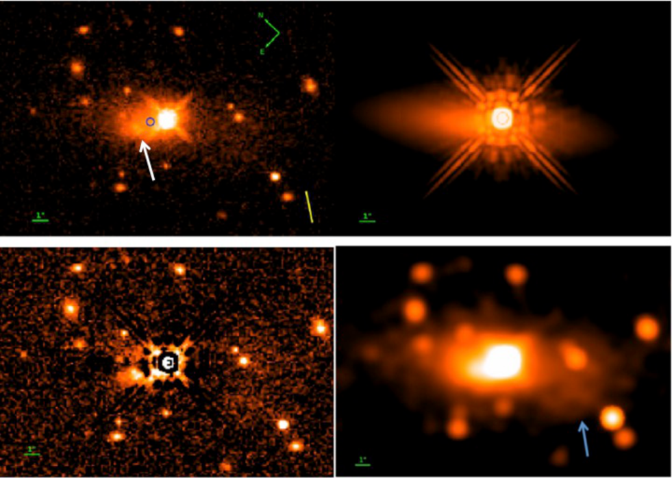
Figure 1: HST image of 3C 186 (top-left). The host galaxy center is indicated with a blue circle. The orientation of the radio jet is shown as a yellow line. The white arrow indicates the location of the so-called blob of unknown origin, $\sim 2$ arcsec East-North-East of the quasar point source. Top-right: model of the source, which includes a PSF and a Sérsic model. Bottom-left: residuals after model subtraction. Bottom right: smoothed (4-pixel kernel) version of the HST image showing the presence of low S/N shells or tidal tails in the host galaxy (indicated by the blue arrow).

Table 1: 2-D modeling best fit parameters

	magF140W	reff	n	e	P.A.
	(1)	(2)	(3)	(4)	(5)
Sérsic	18.86	6.47”	2.57	0.25	37.28
err.	.06	0.61”	0.20	0.01	0.41
PSF	17.39	–	–	–	–
err.	0.01	–	–	–	–

We fit the HST image (Fig. 1, top-left panel) using the 2-D galaxy-fitting algorithm Galfit (Peng et al. 2010). Two components are used in the fit: i) a point-spread function (PSF) to fit the quasar, and ii) a galaxy profile with a Sérsic function (Sersic et al. 1963) for the host galaxy. We use an undistorted PSF model derived with Tinytim (Krist et al. 2011) that was calculated using different power-law spectra with slopes ranging from 0.3 to -1 (F${}_{\nu}\propto\nu^{-\alpha}$) and performing different focus corrections (from f=-0.24 to f=0.91). The observed residuals are only weakly dependent on these parameters. Using both the $\chi^{2}$ and visual inspection of the residuals, we determine that the best results are obtained using $\alpha$=0 and f=0.91. The undistorted PSF model image is oversampled by a factor of 1.3 with respect to the original pixel size, therefore we resampled the image on the same pixel scale using Astrodrizzle. The Tinytim model is not optimal, especially for the core of the PSF, but using a PSF derived from observations of stars in the WFC3 PSF library database (Anderson et al. 2015) does not produce better results in terms of both $\chi^{2}$ and residuals.

We mask out additional sources in the field of view, in a region of about 10$\arcsec$ radius centered on the quasar. Most of these are likely small cluster galaxies at the redshift of the target. Masking out those objects has a significant effect on the output magnitude of the host galaxy only, while the point source flux and position of both components are unchanged. The best-fit model parameters are reported in Table 1. The 2-D model and the residuals after model subtraction are shown in Fig. 1, top-right and bottom-left panels, respectively. One residual blob is visible $\sim 2\arcsec$ East-Northeast of the quasar center. This feature was also masked out during the fitting process. Its origin is not established but, owing to its very blue color, it may possibly be a region of intense star formation, as discussed in Hilbert et al. (2016).

To obtain reliable estimates of the errors on the important parameters, we fixed some of the parameters to values that are slightly different from the best-fit value and we checked the effect on both the $\chi^{2}$ and the residuals. We conclude that the largest uncertainty is in the Sérsic index. If varied between n=1.9 and n=3.7, no effect on the $\chi^{2}$ is seen and very limited changes in the residuals are observed. The results of the analysis show that the quasar PSF is not located at the center of the host galaxy. The offset measured from the best fit is 1.32 $\pm$ 0.05 arcsec, which corresponds to a projected distance of  11 kpc, at the redshift of the source, assuming a scale of 8.244 kpc/arcsec. We also find that fixing the center of the host galaxy to the center of the PSF results in a statistically significant worse fit. In fact, in this case the reduced $\chi^{2}$ increases to 1.292 and the $\chi^{2}$ difference test returns a probability P $<0.005$ than the two fits are the same. Therefore, we conclude that the offset is real.

We note that the effective radius we derive (6.47”, corresponding to 53 kpc at the redshift of the target) is close to the average radius of other well studied BCGs in the same redshift range (i.e. r${}_{\rm eff}=57.3\pm 15.7$ kpc, Stott et al., 2011).

We also note that the host galaxy shows the presence of low surface brightness features that extend to $\sim 6$” south-east of the center of the QSO (Fig. 1, bottom-right panel). These are possibly shells or tidal tails that are typically associated with remnants of galaxy major mergers (Fig. 1, bottom-right panel). Those regions are irrelevant with respect to determining the host galaxy center, because of their extremely low surface brightness. We tried to include a second large-scale component to model this area of the host, but Galfit does not find any meaningful solution. Furthermore, even allowing for the presence of such an additional component, the derived center of the host galaxy is still located at the position derived with the single Sérsic + PSF model discussed above.

3.1.1 Black hole mass estimate

Allowing for some level of uncertainty (typically a factor of $\sim$3), we may infer the mass of the BH by using specific properties of the host galaxy (i.e. stellar central velocity dispersion, bulge luminosity, stellar mass) as indicators. The magnitude of the host galaxy of 3C 186 as derived from our 2-D fit, is m_F140W=18.86 $\pm$ 0.06. Using the WFC3 Exposure Time Calculator tool, we determine that this corresponds to a near IR K-corrected K-band magnitude K=17.1 (in the Vega system), assuming the spectral energy distribution of an elliptical galaxy. Using the relation that links the K-band magnitude to the BH mass (Marconi & Hunt, 2003), we obtain a BH mass of $3\times 10^{9}$ solar masses. This is the expected mass of the SMBH associated with the galaxy we detect in the image.

In Sect. 3.2.4 we also estimate the BH mass using the information derived from the spectra, and we will show that the two values are consistent with each other, within the errors. Furthermore, we use that information to set a tight constraint on the presence of any additional host galaxy around the QSO. This enables us to determine that the host galaxy of the QSO is in fact the one we see in the HST image, which is a very important piece of information to provide a consistent physical interpretation of the data.

3.2 Spectroscopy

3.2.1 Spectral modeling

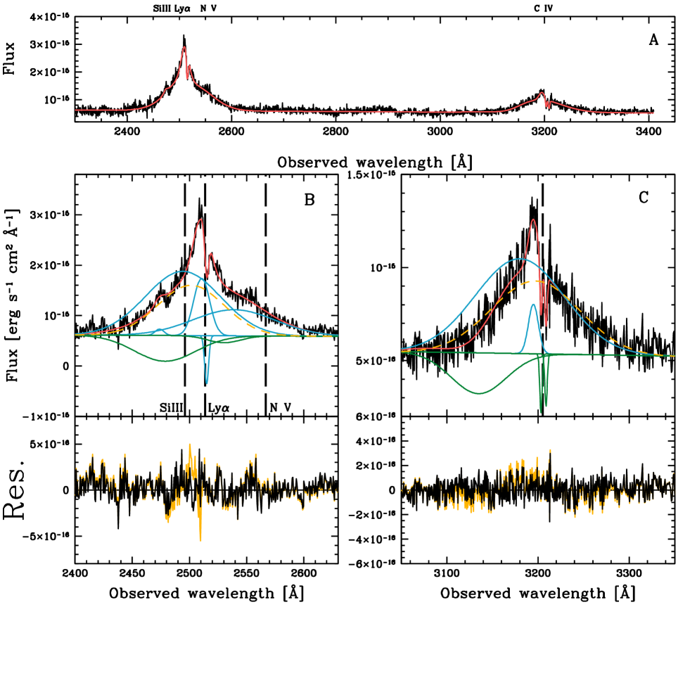
Figure 2: HST/FOS UV spectrum. Wavelengths are in the observer’s frame. In the top panel (A) we show the full spectrum and the best-fit model (red line). Relevant lines are labeled on top of the panel, at the corresponding observed wavelength. The lower panels show zoomed-in regions for each of the lines discussed in the text. Panels B and C show the regions of the Ly$\alpha$ complex and C IV, respectively. The best fit is the red line. Each component of the model is shown separately, added to the continuum power law, for clarity. The emission components are shown in blue and the absorption components are shown in green. Broad components of the best fit derived without including broad absorption are shown as yellow dashed lines. The model residuals are also shown at the bottom of panels B and C. The yellow lines refer to the model without broad absorption. The thick dashed vertical lines correspond to the wavelength of each line at the systemic redshift measured from the narrow lines (see Fig. 3, panel D).

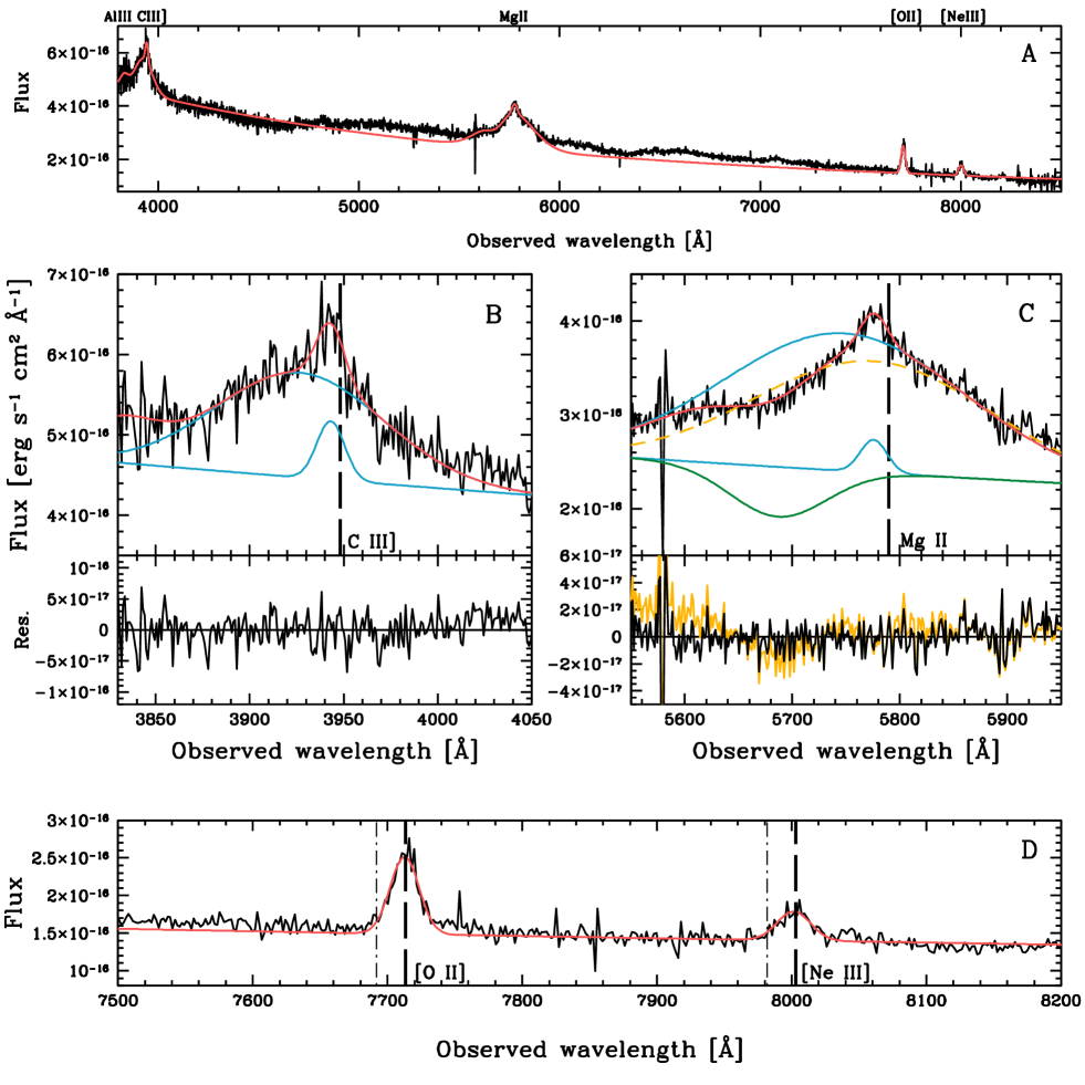
Figure 3: Same as in Fig. 2 but for the SDSS optical spectrum. Panel B and C show the regions of C III] and Mg II, respectively. Note that the continuum in the region of the Mg II line (between $\sim$5000Åand 7000Å) is not reproduced by the fit because of the presence of Fe II features. The best fit is the red line. Each component of the model is also shown, as in Fig 2. The emission components are shown in blue and the absorption components are shown in green. Broad components of the best fit derived without including broad absorption are shown as yellow dashed lines. The model residuals are also shown at the bottom of panels B and C. The yellow lines refer to the model without broad absorption. The thick dashed vertical lines correspond to the wavelength of each line at the systemic redshift measured from the narrow lines (see panel D). Panel D shows the spectral region of the two isolated [O II]3727 and [Ne III]3869 narrow lines. The dot-dashed lines in panel D indicate the wavelengths of these lines corresponding to the redshift of the source estimated by Kuraszkiewicz et al. (2002, see Sect. 3.2.3 for more details).

Spectral fitting is performed using the Specfit tool in IRAF. The spectrum is fit with a global power-law and a collection of Gaussian profiles to each line of interest. The parameters are then successively freed and optimized through a maximum of 100 iterations using a combination of the Simplex and Marquardt minimization algorithms. The optimal parameters for each line are determined until convergence is achieved. The most prominent features in the HST FOS UV spectrum are Ly$\alpha$ and C IV1549 (Fig. 2, panel A). The optical SDSS spectrum shows C III]1909, Mg II2798, [O II]3727 and [Ne III]3869 (Fig. 3, panel A).

The procedure used to derive the best-fit parameters is as follows. We first fit each line complex separately, focusing on the spectral region dominated by each line, to limit the contamination from additional features. This is particularly important for Mg II, to isolate such a line from the possible contamination from Fe II features. At this first step we use the parameters for the continuum power law derived from a first-guess global fit. The best-fit values found for each single line complex is then used in the global fit as first guesses. The errors are estimated from the final global fit.

We checked that the spectral region between $\sim 5600\AA$ and $5700\AA$ (corresponding to a rest frame wavelength range of $\sim 2710-2750\AA$) is not significantly contaminated by Fe II emission. We followed the prescriptions of Vestergaard & Wilkes (2001), i.e. we compared the continuum-subtracted emission of the Fe II features in the pure iron spectral region between 2500 and 2600$\AA$ with the flux level measured in the above range of wavelengths. We derived that the flux immediately blue-ward of the peak of the Mg II line is significantly higher than that expected from Fe II features (by a factor of at least $\sim 2$). A larger contribution from Fe II features is expected red-ward of the Mg II line (around $\lambda_{obs}\sim 6100\AA$) and the observed features are consistent with the expectations in that spectral range.

Broad (FWHM $>$ 3000 km/s) and narrow (FWHM $<$ 3000 km/s) emission and absorption components are used to fit the spectra. The [O II] and [Ne III] forbidden narrow lines are each fit with a single component. Ly$\alpha$, C IV, C III], and Mg II are each fit using broad and narrow emission components. Narrow absorption components are also required for both Ly$\alpha$ and the C IV doublet. For the Ly$\alpha$ complex, the presence of the Si III 1206 line is also apparent, at an observed wavelength of $\sim 2475$Å  (Fig. 2, panel A). In the spectral model of the SDSS data we also include the Al III 1857 line to better reproduce the spectrum blue-ward of the C III] line. This is purely done for cosmetic reasons, since the extremely low S/N ratio at the blue edge of the SDSS spectrum does not allow a clear identification of such a feature.

In addition, for the permitted Ly$\alpha$, N V, C IV, and Mg II rest-frame UV lines, we include a broad absorption component in the spectral model. Such a feature is possibly interpreted as being due to a blue-shifted outflow. Fast, broad absorption features have been recently observed in the UV spectra of a number of AGNs, most notably in NGC 5548 (Kaastra et al., 2014) and NGC 985 (Ebrero et al., 2016). In the following, we show that while in principle these lines can be fitted without broad absorption, including such a component has the effect both of improving the fit with a high statistical significance, and of providing a physically consistent picture of all of the observed emission lines.

The use of a model that includes broad absorption is motivated by the fact that the profile of the broad emission lines appears strongly asymmetric, especially for some of the detected lines. In particular, for both Mg II and C IV, the blue side of the line is clearly concave. The same seems to hold for Ly$\alpha$, but the presence of N V and Si III on the red and blue side of that line, respectively, makes the concave shape less obvious.

While the depression observed blue-ward of the line peak might be a signature of an intrinsic asymmetry of the lines, our choice to fit the spectrum with Gaussian components and to include blue-shifted broad absorption lines is motivated by the following reasons: i) the asymmetry is particularly strong for all the resonant lines, while there is no evidence for any asymmetries in the C III] semi-forbidden line, for which we do not expect broad absorption to be observed; ii) by utilizing Gaussian lines and broad absorption, we can fit all lines with a consistent symmetric profile. Instead, if we were to use asymmetric profiles, each line would have a unique shape that would be difficult to interpret.

Relevant line parameters derived from the best-fit models are displayed in Table 2. In Figs. 2 and 3, panels B and C, we show the best fit spectral model for each line complex (red line). Each of the Gaussian components of the model are shown separately, added to the continuum, in blue and green for emission and absorption, respectively.

To assess the impact of our spectral model assumptions on the results, we also fit the spectra without using a broad absorption component, and we compare the results by performing a $\chi^{2}$ difference test. We simply run Specfit for each of the resonant lines separately, removing the broad absorption component from the fit and freeing all other parameters. The broad emission component derived with this spectral model is plotted in Figs. 2 and 3 as a yellow dashed line. Then we compare the value of $\chi^{2}$ with that obtained using the best fit (with broad absorption) for the same range of wavelengths. For all lines the fit is significantly better when the broad absorption component is used. The significance level, given by the probability that the inclusion of the extra component does not improve the fit, is P$<<$0.001 for both Ly$\alpha$ and Mg II, while for C IV the significance is P$<$0.01. In Figs. 2 and 3, we show a comparison of the residuals of the best fits obtained with and without broad absorption (yellow lines in the residuals box of panels B and C of Fig. 2, and in panel C of Fig. 3). The improvement when broad absorption is used is obvious. When using a model with no broad absorption, the worst fit is obtained in the case of Mg II, where the concavity of the blue side of the line is particularly prominent. In that case, we also try using multiple Gaussian emission components to achieve a better fit, but this type of model does not allow the the fit to converge.

3.2.2 Spectral modeling results: evidence for velocity offsets

The two isolated narrow lines in the SDSS spectrum ([O II] and [Ne III], see Fig. 3, panel D) are the best features to derive the value of the systemic redshift of the host galaxy, since these lines are produced in the narrow line region (NLR) on $\sim$kpc scales, far from the BH. The redshifts of these lines are consistent with each other within 1$\sigma$. By averaging the two redshifts we derive z_h=1.0685 $\pm$ 0.0004. This is consistent with the literature value of z=1.0686 reported by NED (Hewitt & Wild, 2010).

Strikingly, the FOS spectrum shows the presence of a narrow absorption line for Ly$\alpha$, as well as the C IV 1548,1551Å  absorption doublet . The redshift of these three narrow absorption lines is consistent with the systemic redshift of the host z_h derived from [O II] and [Ne III], within 1$\sigma$ and 2$\sigma$ for C IV and Ly$\alpha$, respectively.

All of the observed broad lines show a substantial offset (blue-shift) with respect to the narrow line system. In Figs. 2 (panel B and C) and 3 (panel C) we indicate the wavelengths corresponding to the systemic redshift z_h for each major emission line with thick black vertical dashed lines. This shows the velocity offsets of the broad emission lines very clearly. The offsets of all broad emission components of the major emission lines are consistent with each other within $\sim 1\sigma$ (see Tab. 2).

The measurement with the largest error is obtained for N V, which is a very broad and relatively faint high ionization line that is heavily blended in the Ly$\alpha$ complex. The results for Al III are reported in Table 2 only for the sake of completeness. Even if there is evidence for a significant offset, we believe that the derived value is not reliable for this line because of the extremely low S/N ratio at the red end of the SDSS spectrum.

We use the four strongest broad lines (i.e. Ly$\alpha$, C IV, C III] and Mg II) to derive the average velocity offset v $=-2140\pm 390$ km s^-1. In Fig. 4 we plot the velocity offset against the central wavelength for each of the major broad lines. The data points derived using a broad absorption component in the fit for the resonant lines are shown in red. In blue we show the velocity offsets derived without assuming the presence of broad absorption. We note that even without the inclusion of the broad absorption component, and allowing for a less accurate fit, the broad emission lines are still significantly offset with respect to the systemic wavelength, although the velocity offsets are smaller ($\sim$1000 km/s). However, the CIII] line is still significantly above that value, since no broad absorption is adopted in our analysis for that non-resonant line. Furthermore, we wish to point out that the resulting velocity offsets for each of the lines are not consistent with each other in the case in which no broad absorption is included. Therefore, we conclude that a model with broad absorption components both produces a better representation of the data, and provides a physically consistent picture of the source.

To establish that the assumption of the Gaussian shape for all lines is not artificially generating the line shifts, we perform a measurement of the flux-weighted centroid of the broad component of the C III] line. This is the only broad line included in the available spectra for which we do not expect broad absorption to significantly affect its shape. We masked out both the emission of the narrow component and the region blue-ward of C III], where Al III might contaminate the continuum. Without assuming any specific profile, the broad line is centered at 3920$\pm$15Å, corresponding to z=1.054, and still significantly offset (v$\sim-2140$ km/s) with respect to the systemic redshift z_h.

We also note that each emission line complex is best fitted with the inclusion of a narrow component that is slightly blue-shifted with respect to the systemic redshift. In Table 2, we report each of these lines with a question mark, since their origin is not well determined. These components could be possibly be explained as being due to outflows of moderate velocity ($\sim$100 km s^-1) in the narrow line region.

In Appendix  A we also include first results from a subset of data obtained at the Palomar Observatory 200” telescope with TripleSpec. The only spectral region free of significant atmosphere absorption that includes broad emission lines shows that the He I line is best fitted using a broad absorption absorption component with the same properties as for the UV resonant lines. A more in-depth analysis of the full dataset will be presented in a forthcoming paper.

In summary, our analysis of the spectra show that we can identify two main systems at two different redshifts: the host galaxy (and the NLR) at z$\sim 1.068$, and the broad line region (BLR) at z$\sim 1.054$.

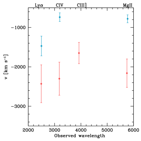
Figure 4: Velocity offsets of the broad emission lines as measured with respect to the systemic redshift z_h plotted against the observed wavelength of each line. The light blue points and the red points are for the spectral models without and with broad absorption, respectively. Note that there is only one point representing the C III] line because for semi-forbidden lines broad absorption is not expected.

Table 2: Emission lines best-fit model

Line component	Observed wavelength	Err.	Redshift	Err.	Velocity offset	Err.	FWHM	Err
	$\lambda$ [Å])		$z$		[km s-1]		[km s-1]
[O II]	7712.7	0.9	1.0686	0.0002	–	–	990	110
[Ne III]	8001.5	2.6	1.0683	0.0006	–	–	1100	250
Si III∗	2474.1	1.5	1.0505	0.0014	-2590	200	1100	450
Ly$\alpha$ (narrow abs.)	2514.9	0.5	1.0695	0.0004	–	–	500	70
Ly$\alpha$ (narrow em.)	2510.9	0.5	1.0662	0.0004	–	–	1980	170
Ly$\alpha$ (broad em.)	2494.3	4.0	1.0525	0.0041	-2430	480	9300	500
Ly$\alpha$ (broad abs.)	2475.4	2.5	1.0368	0.0020	–	–	7630	250
N V∗ (broad em.)	2540.0	10.0	1.0470	0.0081	-3100	1200	10000	800
N V (broad abs.)	2528.3	5.0	1.0376	0.0040	–	–	3600	600
C IV1550 (narrow abs.)	3208.7	0.3	1.0689	0.0014	–	–	300	60
C IV1548 (narrow abs.)	3203.2	0.3	1.0689	0.0005	–	–	300	60
C IV (broad em.)	3180.9	4.4	1.0529	0.0028	-2300	400	10800	560
C IV (broad abs.)	3138.6	5.0	1.0256	0.0032	–	–	6800	760
C IV? (narrow em)	3194.9	1.0	–	–	–	–	1208	360
Al III∗	3828.9	2.8	1.0614	0.0015	-1030	220	3800	150
C III] (narrow em.)	3943.0	1.4	1.0660	0.0005	–	–	1300	150
C III] (broad em.)	3926.6	3.5	1.0572	0.0018	-1640	270	7750	350
Mg II (broad em.)	5748.3	6.9	1.0536	0.0025	-2160	360	13800	470
Mg II (broad abs.)	5687.0	4.5	1.0317	0.0016	–	–	5510	870
Mg II? (narrow em.)	5775.6	1.6	–	–	–	–	1490	330
No broad absorption emission line best fit results
Ly$\alpha$ (broad em.)	2501.4	2.1	1.0583	0.0010	-1470	250	8200	250
C IV (broad em.)	3197.2	1.2	1.0634	0.0008	-739	110	10800	580
Mg II (broad em.)	5775.0	1.7	1.0631	0.0007	-780	100	13500	440

3.2.3 Comparison with previous work

The FOS spectrum was analyzed in Kuraszkiewicz et al. (2002) as part of a large catalog of HST UV spectra of QSOs. Those authors carried out a careful fitting of the UV spectrum of 3C 186 with an automated procedure that uses Gaussian components for all lines and no broad absorption. They derived a systemic redshift of z=1.063, which is inconsistent with the value of z_h we derived. The redshift derived from the Kuraszkiewicz et al. (2002) model is lower than the redshift of the isolated narrow lines we derived from the SDSS spectrum at a significance level of 10$\sigma$. However, the optical SDSS spectrum was not available for them to determine the accurate value of the systemic redshift of the NLR from the isolated narrow [O II] and [Ne III] lines. In Fig. 3, we show the wavelengths at which those lines would be observed if the redshift of the target was z=1.063, as estimated by those authors (the dot-dashed vertical lines in panel D). There are no detected emission lines at these wavelengths, while the [O II] and [Ne III] lines are clearly visible at the wavelengths corresponding to z_h.

3.2.4 Is the QSO associated with an additional (undermassive) host?

From the analysis of the spectroscopic data we are able to infer the virial BH mass of the QSO. We use the FWHM of the Mg II line as an estimator (Trakhtenbrot & Netzer, 2012), to limit any biases due to the possible contamination of winds that might affect high-ionization UV lines, and we obtain M_BH= $6\times 10^{9}$ solar masses. We note that Kuraszkiewicz et al. (2002) estimated the black hole mass for this source using C IV, and derived a similar mass ($3\times 10^{9}$ M_☉). The virial BH mass estimate is thus consistent with that based on the host galaxy magnitude (Sect. 3.1.1) within the uncertainties of the used relations. Furthermore, a rough lower limit on the black hole mass can be derived using the assumption that the BH accretes at the Eddington limit. For L${}_{\rm bol}\sim 10^{47}$, the lower limit on the BH mass is $8\times 10^{8}$ M_☉.

The fact that such a value is consistent with the BH mass derived from the galaxy magnitude shows that the two objects perfectly match the expected properties for a QSO and its host galaxy. However, for the purpose of providing a more robust physical picture of the system, it is important to firmly establish that a model that includes one PSF and one galaxy (hereinafter galaxy #1) is the best representation of the HST image and thus the host galaxy we see is the only galaxy associated with the QSO. To this aim, we perform a set of additional tests and simulations using Galfit.

Firstly, we include a second Sérsic component (galaxy #2) in the model and fixed its center to be co-spatial with the center of the PSF. When all the parameters are left free to vary except for the centers of each of the three components, the fit does not have a constrained solution for galaxy #2. The resulting magnitude of galaxy #2 is only a lower limit (m${}_{\rm F140W}>24.42$, i.e. $\sim$ 100 times fainter than the expected luminosity of the host galaxy of a $\sim 6\times 10^{9}$ M_☉ BH), and the resulting r_eff is $\sim$ 200″, which corresponds to $\sim$1.6Mpc at the redshift of the object. Clearly this solution is unphysical. Furthermore, the reduced $\chi^{2}$ worsens significantly. Most notably, the properties of both the PSF and galaxy #1 are unchanged with respect to the best-fit model that includes only two components.

Secondly, we add a simulated elliptical galaxy (Sérsic index n=4, ellipticity e=0.5, effective radius r_eff=3″) obtained using the package artdata within IRAF to test whether Galfit is able to correctly identify the presence of an object significantly fainter than galaxy #1. The simulated galaxy is four times (1.5mag) fainter than the detected host, i.e. significantly fainter than the luminosity expected from the correlation of M_BH with the host magnitude (Marconi & Hunt, 2003), even taking into account of its dispersion ($\sim$ 0.3 dex). When this additional component is superimposed onto the PSF, Galfit is able to correctly fit the image, with a $\chi^{2}$ consistent with that of our best-fit model. Therefore, if such a galaxy were present in the image, Galfit would have been able to detect it.

We also simulate a smaller (r_eff=1″) spheroid with the same magnitude as in the previous simulation, and we superimpose that to the QSO. Galfit is again able to fit such a component, but with a larger error on both the effective radius and the Sérsic index. Therefore, even in the case of the lower BH mass estimate that was derived assuming accretion at the Eddington limit, the expected host galaxy would still lie within the range that we could detect with our method, based on the tests performed above.

We conclude that, even if the presence of an under-luminous object cannot be completely excluded, the best model to fit the image includes two components only: one PSF and one elliptical galaxy. Any additional galaxy at the location of the PSF would be significantly under-luminous (possibly by a factor of more than 100, according to our first test) with respect to its expected luminosity, given the BH mass of the QSO. This directly implies that such a scenario is very unlikely.

3.3 X-ray Chandra-ACIS data

We analyzed archival Chandra X-ray observations to evaluate the possibility of a second AGN located at the coordinates corresponding to the isophotal center of the host galaxy. We register the Chandra 0.5-7 keV image to the world coordinate system of the HST WFC3-IR image, using the peaks of the emission in the two images (i.e. the position of the unresolved quasar). In registering the Chandra image to the framework of the HST image, we assume that the bright point sources in each image are both associated with the QSO, and that they are co-spatial.

We take into account the contributions from the quasar (and the associated PSF of the ACIS-S instrument), the cluster and the background.

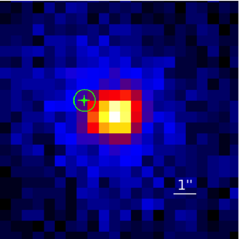
Figure 5: Chandra X-ray image of 3C 186. The bright point source at the center of the field of view is the quasar. The region marked with the circle corresponds to the location of the galaxy nucleus, where the upper limit for any additional AGN source was estimated. In this figure North is up and East is left.

We estimate a 3$\sigma$ upper limit F${}_{\rm 2-10keV}<2.2\times 10^{-15}$ erg cm^-2 s^-1 for a second AGN, in a circular region with one pixel radius centered at the coordinates corresponding to the host galaxy center (Fig. 5). This value corresponds to a 2-10 keV luminosity L${}_{\rm 2-10keV}=1.3\times 10^{43}$ erg s^-1 at the redshift of the source. This is $\sim$100 times lower than the luminosity measured for 3c186 (L${}_{\rm 2-10keV}=1.2\times 10^{45}$ erg s^-1). Assuming that any AGN at the center of the host is strongly obscured in the X-rays we can correct its observed X-ray flux for an average factor (Marinucci et al. 2012) of 70, leading to an upper limit of L${}^{\rm C-thick}_{2-10keV}<9.1\times 10^{44}$ erg s^-1. We also note that the power needed to photo-ionize the narrow emission lines as estimated from L_[OIII] (Hirst et al., 2003) is L${}_{\rm 2-10keV}=7.3\times 10^{45}$ erg s^-1, using the relation between these two quantities (Heckman et al. 2005). This implies that if the observed QSO and the galaxy were a chance projection, the presence at the center of the host of an AGN that is powerful enough to photo-ionize the observed narrow lines would be detected at $>3\sigma$ level, even if Compton-thick absorption was present, under reasonable assumptions.

4 Discussion

We presented evidence for both a spatial offset between the nucleus of 3C 186 and its host galaxy, and a velocity shift between the broad and narrow emission lines in its spectrum. In the following we discuss possible interpretations of our results. We first consider scenarios that assume that the velocity offsets are caused by peculiar properties of the central AGN, i.e an extreme disk emitter or a peculiar wind. We then discuss scenarios that can possibly account for both the velocity and spatial offsets displayed by this source. We then outline the reasons why we believe that the interpretation as a GW recoiling BH is favored when accounting for the overall properties of this object.

4.1 An extreme disk emitter

The velocity offsets observed in the spectra of 3C 186 can, in principle, be explained in terms of extreme asymmetries of either the broad line region or the accretion disk. One possibility is that 3C 186 represents an extreme case of an eccentric disk emitter (e.g. Eracleous et al., 1995). Peculiar line profiles and double-peaked broad low-ionization lines are found in a fraction ($\sim 10\%$) of radio-loud AGNs (e.g. Eracleous et al., 2003; Strateva, 2004; Liu et al., 2016). Extreme cases of double-peaked lines in which the blue peak dominates may mimic the features observed in 3C 186.

However, there are a number of problems with such an interpretation:

i) eccentric disk models predict that the apparent velocity shifts observed in low and high ionization lines (e.g. Mg II and C IV, respectively) should be different, since the low-ionization lines are produced in the higher density accretion disk (thus originating the double-peaked Balmer lines) while the higher ionization lines are thought to be produced in a low density wind (Murray & Chiang, 1997; Chen & Halpern, 1989; Eracleous et al., 2003; Strateva, 2004; Braibant et al., 2016). In fact, Ly$\alpha$ and C IV are always single-peaked in objects with double-peaked Balmer and Mg II lines (e.g. Halpern et al., 1996). On the other hand, the observations of 3C 186 presented here show that, for this object, all broad lines (of both low and high ionization) are shifted. Furthermore, in the model in which broad absorption is used, all velocity offsets are consistent with the same value;

ii) objects with double-peaked and strongly asymmetric lines are known to show significant variability both in the emission line profile and flux (e.g. Eracleous et al., 1997; Gezari et al., 2007; Liu et al., 2016), because of the intrinsic asymmetric structure of the accretion disk and the possible effects of winds. The spectra we use in our analysis were taken nine years apart. The overlap between these two spectra is small, since only the C III] line was observed at both epochs. The HST/FOS data are extremely noisy in the C III] region, and do not add any significant information because a fit would be poorly constrained. However, we checked that the model parameters we use to fit the C III] line in the SDSS spectrum also provide a good representation of the same line in the HST/FOC data. We also note that the continuum emission in the region in which the spectra overlap is also consistent with being stable. While we cannot completely exclude that variability is present, it is striking that all of the broad lines show consistent offsets, considering that the two spectra were taken nine years apart.

4.2 A peculiar wind

The specific properties of the broad line offsets in 3C 186 could also be interpreted in the context of a wind scenario. The presence of winds is often used to explain significant blue-shifts characterizing high-ionization lines in the spectra of quasars. Using a large sample of SDSS quasars, Shen et al. (2016) show that high-ionization broad lines such as C IV are generally more blue-shifted than those of low ionization (such as Mg II). In turn, low-ionization permitted broad lines do not show large velocity offsets with respect to low ionization narrow lines that are best used to derive the systemic redshift of the object (such as e.g. [O II]). Typical velocity offsets with respect to low ionization narrow lines are of the order of a few tens of km s^-1 for Mg II, with an intrinsic spread of $\sim 200$ km s^-1. Therefore, in most cases Mg II can be considered as a good indication of the systemic redshift of the object.

Offsets displayed by C IV with respect to Mg II show strong luminosity dependence. However, such a relation is less strong and the velocity offsets are, on average, smaller for radio-loud QSOs (Richards et al., 2011). Shen et al. (2016) show that for bright QSOs, the average blue-shift of C IV is $\sim 700$ km s^-1, with a scatter of $\sim 100$ km s^-1.

While the properties observed in the spectra of 3C 186 can be qualitatively explained in the framework of a disk-wind model, the offsets we measure are rather atypical, since we have both high (e.g. C IV) and low (Mg II) ionization lines that show similar blue-shifts. Velocity offsets as high as those that we measure in our source are also extremely rare in the general QSO population. This is particularly evident for low ionization lines such as Mg II for which, even using the spectral model that assumes no broad absorption, the derived velocity offset is $>3.5\sigma$ higher than those shown by the SDSS QSOs (Shen et al., 2016).

Based on these considerations, we conclude that a scenario that explains the data with a peculiar disk or disk+wind models cannot be completely ruled out, but is unlikely. Furthermore, we note that, while such a scenario might in principle account for the velocity offsets observed in some (but not all) of the emission lines, it does not explain by itself the spatial offset observed in the image. To explain the properties of the spectrum of 3C 186 in the context of a disk/wind scenario, we would also have to assume that the QSO is disconnected from the galaxy we see in the HST image, and it is in-falling towards that galaxy at a velocity of the order of at least $\sim 1000$ km/s, to account for the velocity offset displayed by the Mg II line.

In the following we further discuss this type of scenario, and we outline our favored interpretation for both the spatial and the velocity offsets in the context of a single framework, without assuming any specific intrinsic peculiarity of the QSO.

4.3 How do we explain both spatial and velocity offsets?

Four different scenarios may account for both intrinsic velocity and spatial offsets: i) the quasar and the detected galaxy are two unrelated systems located at different redshifts (with the quasar being a foreground object, as the broad lines are blue-shifted); in this case, both objects are AGNs (one produces the broad lines, the other one produces the narrow lines only); ii) same as above, but with the QSO as a background object that is moving towards the detected galaxy; iii) a recoiling (slingshot) BH resulting from the interaction of a double or multiple BH system in the host, in which at least another BH is active to produce the narrow lines (i.e. a dual or multiple AGN); and iv) a GW recoiling black hole.

Regarding the first scenario, the detection of UV absorption lines in the quasar spectrum at a systemic velocity consistent with that of the narrow emission lines directly implies that the QSO cannot be a foreground object. The velocity offset derived using our model that includes broad absorption is significantly ($\sim 3\sigma$) larger than the velocity dispersion of the cluster in which the object resides ($\sigma=780$ km/s), as estimated from the properties of the X-ray cluster emission (Siemiginowska et al., 2010). The possibility that the QSO is a cluster object in the background that is in-falling towards the detected galaxy (second scenario) is thus unlikely. If we assume that broad absorption should not be used to fit the emission lines (but see Sect. 3.2.2 for a discussion on why we believe this would not be the best model), then the velocity offsets of all resonant lines (i.e. all but C III]) are closer to the cluster velocity dispersion. Therefore, in this scenario, the possibility that the QSO is a background object, which is in-falling towards the galaxy we see in the HST image, cannot be rejected. However, there are still two issues to be explained. Firstly, the lack of a substantial host galaxy of the QSO, which should be significantly undermassive in order to be undetected, as shown in Sect. 3.2.4. Secondly, and most importantly in such a scenario, the presence of two AGNs must be assumed, one that produces the broad lines, and one that produces the narrow line system at z_h. The presence of a Type 2 (hidden) AGN at the center of the detected galaxy could, in principle, explain the narrow line system at z_h. In this scenario, we would also expect to see a bright set of narrow lines associated with the NRL of the QSO, at a redshift consistent with that of the broad emission lines. These lines are clearly absent from the spectrum (see Fig. 3, panel D).

The interpretation of the data in terms of a dual or multiple AGN (third scenario) is also very unlikely considering the power of the ionizing source needed to produce the observed emission from the NLR. This can be estimated from the luminosity of the [O III]5007 line L${}_{\rm[OIII]}=2.2\times 10^{44}$ erg s^-1 (Hirst et al., 2003). We derive L${}_{\rm bol}\sim 7.5\times 10^{46}$ erg s^-1, using appropriate scaling relations (Punsly & Zhang 2011). This is consistent with the luminosity of the quasar L${}_{\rm bol}\sim 10^{47}$ erg s^-1 as measured by Siemiginowska et al. (2010), and directly implies that the QSO is sufficient to photo-ionize the observed narrow lines. Given these considerations, we infer that, not only an additional AGN is not required but, based on the analysis of Chandra data, we can also rule out the presence of another powerful unobscured or mildly obscured AGN located at the isophotal center of the host. In fact, the upper limit to the X-ray emission of any other accreting BH at the position corresponding to the center of the host is about two orders of magnitude lower than the power needed to photo-ionize the observed narrow emission lines. The presence of a typical heavily obscured (Compton-thick) AGN is also very unlikely. In fact, the 3$\sigma$ upper limit for the X-ray intrinsic luminosity derived in Sect. 3.3 is a factor of $\sim$8 lower than the power of the Compton thick AGN needed to photo-ionize the narrow lines.

Furthermore, the presence of additional SMBHs in the system is unnecessary to explain the observations. The BH mass derived using the host galaxy magnitude converted to the (rest-frame) infrared K-band as an indicator (Marconi & Hunt, 2003) is M${}_{\rm BH}=3.0\times 10^{9}$ M_☉. The virial mass estimate derived using the FWHM of the Mg II line line (Trakhtenbrot & Netzer, 2012) returns a similar value ($6\times 10^{9}$ M_☉). Thus, the presence of another BH is not necessary, since the one associated with the QSO has the mass we expect based on the properties of the host in which it resides. In turn, this also implies that if the quasar resided in a host galaxy other than the one detected in the HST image, the host galaxy associated with such a massive BH would be detectable, at least in the model residual image, as shown in Sect. 3.2.4.

We note that a dual AGN (or AGN + inactive BH) scenario is also unlikely because of the observed large velocity offset. Expected velocity offsets for dual AGNs are of the order of 10 to 100 km/s (e.g. Wang & Yuan 2012, Comerford & Greene 2014). Furthermore, the Keplerian velocity for a $\sim 10^{9}$ M_☉ BH in a binary system, at a distance of $\sim$10kpc from the other component would be of the order of a few tens of km s^-1, clearly inconsistent with the observations.

Finally, the presence of a single host galaxy also disfavors a pre-merger black hole binary or, even less likely, of a slingshot effect due to a three-body interaction. In this scenario we would expect to observe a galaxy merger still in progress.

We conclude that the most likely explanation is the fourth scenario, which involves a GW recoiling black hole. While we admittedly cannot completely exclude that an ad hoc combination of some (or all) of the above discussed scenarios could conspire to give rise to the observed properties of our object, the GW recoiling BH scenario naturally accounts for both the observed velocity and spatial offsets. Furthermore, it does not require any ad hoc assumptions on the specific properties of host galaxy, BLR and NRL of this quasar. In this scenario, 3C 186 would then be a normal QSO, which simply happened to be ejected from its host galaxy by a well known mechanism that is expected, in some cases, as a result of a BH merger (e.g. Peres, 1962; Loeb, 2007; Volonteri & Madau, 2008).

4.4 A GW recoiling black hole

Having explored a number of possible explanations to account for the observed properties of 3C 186, we favor the GW recoiling BH scenario. The SMBH was likely ejected as a result of the gravitational radiation rocket effect, following a major galaxy merger in which the SMBHs at the center of each merging galaxy also merged. The accretion disk and the broad line region remained attached to the recoiling BH. The narrow emission lines are produced at larger distances from the BH with respect to the BLR, in the systemic frame of the host galaxy. This scenario explains the observed velocity offsets between the broad and narrow emission line systems. Furthermore, it also accounts for the observation of the nuclear spatial offset with respect to the isophotal center of the host galaxy.

The measured velocity offset is close to or slightly higher than the escape velocity expected for a massive elliptical galaxy (e.g. Merritt et al., 2004). High-velocity offsets (v$>$1000 km/s) are expected to be rare and they are more likely to be observed in combination with large spatial offsets (Blecha et al., 2016). In Fig. 6, we show a comparison between the velocity and nuclear offsets measured in some of the most interesting GW recoiling BH candidates published so far. We note that one of them (SDSS 0956+5128) displays even larger velocity shifts than 3C 186. However, in this case, the fact that the low-ionization broad permitted lines (H$\beta$ and Mg II) show significantly different shapes cannot easily be explained in terms of a recoiling BH (Steinhardt et al., 2012). 3C 186 is one of the highest velocity objects, but it is also the one object that shows the largest spatial offset.

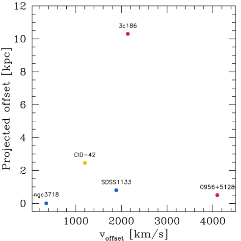
Figure 6: Projected spatial offset plotted against broad to narrow emission line velocity offsets (absolute value) in recoiling black hole candidates. The color scale reflects the bolometric power of each object. Blue is used for L${}_{\rm bol}<10^{43}$ erg s^-1, yellow for $10^{43}<$ L${}_{\rm bol}<10^{45}$ erg s^-1 and red for L${}_{\rm bol}>10^{45}$ erg s^-1. For SDSS1133 the velocity offset is known to vary between  40 km/s and  1890 km/s (Koss et al., 2014). In this figure we use the measurement corresponding to the highest velocity.

4.4.1 Relevant timescales and effects on the observed radio and optical morphologies

The first important timescale we can derive from the observations is the time since the GW kick was received as the two BHs merged. Given the measured velocity of $\sim 2100$ km s^-1 and the 1.3” spatial offset, we derive that the time since the BH merger event is $\sim 5$Myr, assuming both a constant velocity and that the angle between the direction of motion and the line-of-sight is $\sim$45deg.

An important property of 3C 186 is that it possesses powerful relativistic jets. The presence of radio jets allows an estimate of the age of the SMBH activity, based on the synchrotron radiative cooling timescale. Murgia et al. (1999) estimated a radiative age of $\sim 10^{5}$ years for 3C 186. This implies that the radio AGN turned on at a later time with respect to the time of the GW kick. We note that since the radio source is very young we do not expect to see any significant bending in the radio jet as a result of the BH motion. Assuming a projected velocity of the order of that measured from the spectra ($\sim 2100$ km ^-1), any displacement of the hot-spots with respect to radio core would be less than 0.1”. This is consistent with the observed radio morphology, in which the jet appears roughly straight (Spencer et al., 1991). However, the hot-spots are slightly displaced with respect to the jet direction, displaying an S-shaped morphology. This type of radio morphology is usually interpreted as being due to a jet emitted by a precessing BH (Ekers et al., 1978), which is to be expected as a result of a BH merger with misaligned spins and/or uneven BH masses.

We can also estimate the lifetime of an accretion disk attached to a BH kicked at a velocity $\sim 2100$ km s^-1. Using the formula in Loeb (2007), and assuming a radiative efficiency of $\epsilon=0.1$ and the luminosity and BH mass estimated for 3C 186, we derive t${}_{\rm disk}\sim 10^{8}$ yr. This is a significantly longer timescale than the time since the GW kick occurred. This implies that the accretion disk can survive until the BH reaches very large distances from the center of the host, thanks to the fact that its lifetime strongly depends on the BH mass.

The host galaxy shows the presence of low surface brightness features in its outer regions, possibly shells or tidal tails that are typical of major galaxy merger remnants, i.e. those in which the two merging galaxies have masses that are equal to within a factor of 3 (Fig. 1, bottom-right panel). From a qualitative comparison with simulations (e.g. Springel et al., 2005; Lotz et al., 2008), we estimate that the galaxy merger event happened on timescales of about 1Gyr or more, since only one distinct galaxy with a relatively smooth morphology is visible. Furthermore, the Sérsic index resulting from the fit is consistent with that of relaxed elliptical galaxies.

A quantitative comparison is extremely difficult with the current data because of the complexity of the problem, as well as the low S/N of the image in the outer regions of the host galaxy, which prevents us from disentangling the faint structures in the possible tidal tails. Simulations (e.g. Lotz et al. 2008) show that the expected morphologies at different times since the beginning of the merger are strongly dependent on the initial parameters (i.e. mass, gas content, galaxy morphology). However, it is clear (e.g. Figs. 1 and 2 in Lotz et al. 2008) that for t$<$1-2Gyr the central regions of the merged galaxy are still significantly disturbed. This is not what we observe in the host of 3C 186, where the galaxy can be accurately modeled with a smooth Sérsic component. Thus, the galaxy merger must have occurred more than 1-2 Gyr ago.

It is possible that when the target is observed with higher resolution instruments we may be able to see more details in the innermost kpcs. But since the spatial resolution offered by HST/WFC3 is $\sim 0.8$ kpc at the redshift of the source, we believe that significant disturbances would be visible in our data (see, for example, the morphologies of some of the merging 3C radio galaxies presented in Chiaberge et al. 2015).

Finally, we note that in a galaxy merger in which both galaxies possess an SMBH, the timescale for two SMBHs to sink into the center of the merger remnant and form a bound binary is likely at least one order of magnitude shorter than the timescale of 1-2 Gyr (or more) that we roughly estimate for the galaxy merger (e.g. Begelman et al., 1980; Khan et al., 2012). This implies that if we assumed that the two BHs in the 3C 186 merging system have not merged yet, and that what we are observing is a SMBH binary system, the observed large velocity offsets would be inconsistent with the small velocities expected for a BH binary (see Sect. 4.3).

5 Conclusions

Irrespective of the specific interpretation of the results, 3C 186 is an extremely interesting and unique object. We measure a spatial offset of $1.3^{\prime\prime}$ between the QSO point source and the isophotal center of the host galaxy. This corresponds to a projected distance of $\sim 11$kpc at the redshift of the source. The broad emission lines show significant velocity offsets (v$\sim 2100$ km s^-1) with respect to the systemic redshift of the host galaxy as derived from the narrow emission and absorption line system. We showed that the most plausible explanation for both the nuclear spatial offset seen in the HST/WFC3-IR image and in the spectra is in terms of a gravitational wave recoiling black hole scenario, although the explanation in terms of a peculiar background QSO associated with an undermassive host galaxy and/or characterized by peculiar winds cannot be completely excluded. Based on the morphology of the host, we estimate that a major merger between two galaxies both containing an SMBH occurred roughly $1-2$ Gyr ago. When the BH-BH merger occurred, probably $\sim 5\times 10^{6}$ years ago based on both the observed velocity and spatial offsets, the anisotropic emission of gravitational waves generated a kick that ejected the merged SMBH from the central region of the merged host galaxy. The AGN accretion disk remained attached to the BH, thus causing the observed velocity offsets of the broad emission lines with respect to the NLR. Spectral aging arguments show that the radio-loud AGN turned on more recently, $\sim 10^{5}$ years ago (Murgia et al., 1999). Theoretical considerations (Loeb, 2007) have been made that indicate that the accretion disk can survive in such a condition for a timescale of as long as $\sim 10^{8}$ years.

3C 186 is a perfect laboratory to study all of the effects associated with galaxy and BH mergers, the timescales involved in these processes, and the production of gravitational waves. The fact that this object is radio-loud is extremely interesting. On the one hand, some of the best models to explain the production of relativistic jets require the presence of a rapidly spinning BH (e.g. Blandford & Znajek, 1977; McKinney et al., 2012; Ghisellini et al., 2014). On the other hand, there is growing evidence that RLAGNs are closely linked to major galaxy and BH mergers (Wilson & Colbert, 1995; Ivison et al., 2012; Ramos Almeida et al., 2013; Chiaberge et al., 2015). Interestingly, one possible way to spin-up the black hole is via a BH-BH merger with specific spin configurations (e.g. Schnittman, 2013; Hemberger et al., 2013). Therefore, it is not surprising that we are able to observe a GW recoiling SMBH associated with a radio-loud AGN.

A number of future studies of 3C 186 should be performed to further investigate the properties of this intriguing source and test the proposed GW recoiling black hole scenario. Deeper HST images will allow us to both completely rule out the presence of an under-massive host galaxy around the QSO, and to better study the properties of the galaxy merger remnant. This should include color information, to determine the age of the stellar populations at different locations in the host galaxy, and set constraints on the galaxy merger timescales. Spectroscopy at UV and optical wavelengths will enable the monitoring of the spectral features we observed, which is crucial to determine whether these are transient or permanent phenomena. High-resolution spectroscopy with high S/N will also enable a more accurate measurement of the line offsets. Observing the spectral region of the H$\beta$ emission line would provide a cleaner picture of the low-ionization BLR, since such a line is significantly less contaminated by other spectral features with respect to the Mg II UV line and the other lines presented here. If the GW recoiling BH scenario holds, we expect the broad H$\beta$ line to show a velocity offset consistent with those measured in the lines presented in this paper (i.e. $\sim 2000$ km/s). IFU data taken with an 8m-class telescope and adaptive optics will enable us to identify the spatial location of the NLR, and to observe the expected decoupling of the BLR and NLR.

Furthermore, ALMA observations will enable the study of the kinematics of the molecular gas in the vicinity of the recoiling BH and at the center of the host galaxy. Future X-ray observations with space-based X-ray high-resolution spectrographs, such as the one that will be on board the planned ESA X-ray telescope Athena, will allow direct measurements of (or put stringent limits on) the BH spin in this source. Numerical modeling will also be extremely important to better understand important issues, from the triggering mechanisms of radio loud AGNs to their connection with merging BHs.

Finally, if the GW recoiling BH scenario is correct, these results are clearly also relevant for gravitational wave studies. GWs from $\sim$30 M_☉ merging BHs were recently detected by LIGO (Abbott et al. 2016) and pulsar timing experiments (EPTA, PPTA, and SKA in the future) will in the future be able to detect GWs of the frequency expected from mergers of BHs with masses similar to that of 3C 186 (Moore et al. 2015, Babak et al. 2016, Madison et al. 2016).

Appendix A Palomar TripleSpec data: preliminary results

A.1 The data

We obtained a spectrum of 3C 186 with the Palomar 200” Telescope and TripleSpec in the J, H and K near-IR bands. The spectrograph sensitivity curve extends from $\sim$ 1.0 to 2.4 $\mu$m, and the spectral resolution varies between 2500 and 2700, depending on the wavelength. The data were taken on December 10-12, 2016. Here we present data from the first part of the observation, and we focus on the J- and K-band spectra, which include information relevant to this paper. The full dataset will be presented in a forthcoming paper. The exposure time was 245 minutes,using an A-B-B-A sequence. Calibration data were also taken during the same nights, including flats, darks and calibration stars for telluric subtraction and flux calibration. The spectrum was reduced and calibrated using SpexTool (Cushing et al., 2004). Telluric absorption bands cover spectral regions that, at the redshift of the source, include both H$\alpha$ and H$\beta$. Therefore, the major broad emission lines that fall in the near-IR, as accessible from ground-based telescopes, are He I 10830 and Paschen $\gamma$ (see e.g. Riffel et al., 2006). Paschen $\delta$ is also detected, but it is significantly fainter and falls in a noisier region of the spectrum. These lines all fall in order 3 of the spectrum, which corresponds to a spectral region between $\sim$ 1.9 and 2.4 $\mu$m. Order 6 of the spectrum includes the [O III]5007,4959 doublet.

Figure 7: Palomar TripleSpec spectrum (order 6). Wavelengths are in the observer’s frame. The [O III]5007,4959 doublet is shown. The vertical dashed lines indicate the wavelengths of these two lines corresponding to the systemic redshift z${}_{h}=1.0685$.

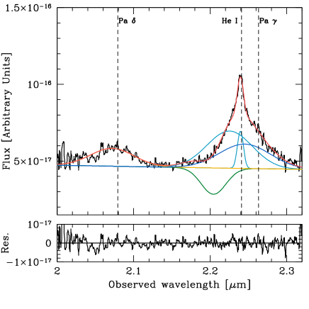
Figure 8: Palomar TripleSpec spectrum (order 3). Wavelengths are in the observer’s frame. Relevant lines are labeled at the top of the panel. The vertical dashed lines indicate the wavelengths of the lines corresponding to the systemic redshift z${}_{h}=1.0685$. The best fit is the red line. Each component of the model is shown separately, added to the continuum power law, for clarity. The emission components are shown in cyan and blue for He I and Pa $\gamma$, respectively. The absorption component is plotted in green. Model residuals are shown in the bottom panel.

A.2 Results

The relevant segments of the Palomar TripleSpec spectrum are shown in Figs. 7 and 8. In Fig. 7 we show the spectral region around the [O III]5007,4959 doublet. The dashed vertical lines show the wavelengths of these two emission lines corresponding to the systemic redshift z${}_{h}=1.0685$. It is clear that both lines are centered at z_h, in agreement with the [O II] and [Ne III] lines detected in the SDSS spectrum (see Sect. 3.2.2). Fitting this region is rather complex because of the presence of the red side of the broad H$\beta$ line, visible as a rising component blue-ward of the [O III]4959 line. Unfortunately, atmospheric absorption combined with the reduced sensitivity of the spectrograph at $\lambda<1\mu$m do not allow accurate modeling of the H$\beta$ line, thus both the peak wavelength and width are unconstrained. However, the central wavelengths of the [OIII] emission lines can be accurately measured. In Fig. 8 we show the spectral region of the He I line. The line is blended with Paschen $\gamma$. The Paschen $\delta$ line is also detected, but it is significantly fainter. The shape of the strongest line (He I) is similar to that of the UV broad resonant lines (i.e. the blue side of the line shows a concave profile).

We model the lines using the same technique as described in Sect. 3.2.1. In Table 3 we report the results of the best fit. In model A, we adopt a set of narrow and broad emission lines with one broad absorption component for He I, in analogy with the UV broad resonant lines and to better reproduce the concave line profile. He I and Paschen $\gamma$ are offset by $\sim 2200$ km/s with respect to the systemic redshift. The Paschen $\delta$ line shows a smaller offset (i.e. 1050 km/s). However, the signal-to-noise for this line is significantly lower because of the presence of the strong carbon dioxide absorption features at $\sim$2.06 $\mu$m. Furthermore, for such a line we do not include a broad absorption component. In model B we fit the He I complex without including a broad absorption component. Significant offsets are still present ($\sim 1500$ km/s). However, the quality of the fit is significantly lower and the errors are larger. We compared the $\chi^{2}$ derived for each model and we obtain that the model with broad absorption better represents the data with a high level of statistical significance (P $<<$ 0.001). We note that He I also shows a narrow emission component that is offset by $\sim 200$ km/s, again in agreement with the narrow components observed in the UV resonant lines (see Tab. 2).

We conclude that these preliminary results support the presence of significant velocity offsets, in quantitative agreement with those derived for the UV emission lines in Sect. 3.2.2.

Table 3: Emission lines best fit model parameters, Palomar TripleSpec data

Model A: With broad absorption component
Line component	Observed wavelength	Err.	Redshift	Err.	Velocity offset	Err.	FWHM	Err
	$\lambda$ [Å])		$z$		[km s-1]		[km s-1]
He I (broad em.)	22252	8.3	1.0540	0.0004	-2100	110	9400	150
He I (broad abs.)	22042	4.5	1.0347	0.0002	–	–	5200	60
He I (narrow em.)	22395	1.0	1.0672	0.0001	-190	10	1200	50
Paschen $\gamma$	22450	9.8	1.0520	0.0004	-2400	130	10500	100
Paschen $\delta$	20720	5.1	1.0612	0.0003	-1100	200	9700	250
Model B: No broad absorption component
He I (broad em.)	22309	22.0	1.0593	0.0010	-1320	300	11200	300
He I (narrow em.)	22382	1.5	1.0686	0.0001	-360	10	2400	50
Paschen $\gamma$	22502	40.0	1.0566	0.0020	-1700	500	9100	100
Paschen $\delta$	20720	6.0	1.0613	0.0003	-1050	90	11100	200