Balanced truncation and singular perturbation approximation model order reduction for stochastically controlled linear systems

Abstract

When solving linear stochastic differential equations numerically, usually a high order spatial discretisation is used. Balanced truncation (BT) and singular perturbation approximation (SPA) are well-known projection techniques in the deterministic framework which reduce the order of a control system and hence reduce computational complexity. This work considers both methods when the control is replaced by a noise term. We provide theoretical tools such as stochastic concepts for reachability and observability, which are necessary for balancing related model order reduction of linear stochastic differential equations with additive Lévy noise. Moreover, we derive error bounds for both BT and SPA and provide numerical results for a specific example which support the theory.

Keywords:

model order reduction, balanced truncation, singular perturbation approximation, stochastic systems, Lévy process, Gramians, Lyapunov equations.

AMS Subject Classifications

Primary 93A15, 93B40, 93E03, 93E30, 60J75. Secondary 93A30, 15A24.

1 Introduction

Many mathematical models of real-life processes pose challenges during numerical computations, due to their large size and complexity. Model order reduction (MOR) techniques are methods that reduce the computational complexity of numerical simulations, an overview of MOR methods is provided in [1, 28]. MOR techniques such as balanced truncation (BT) and singular perturbation approximation (SPA) are methods which have been introduced in [21] and [19], respectively, for linear deterministic systems

$$\dot{x}(t)=Ax(t)+Bu(t),\quad y(t)=Cx(t).$$

Here $A\in\mathbb{R}^{n\times n}$ is asymptotically stable, $B\in\mathbb{R}^{n\times m}$, $C\in\mathbb{R}^{p\times n}$ and $x(t)\in\mathbb{R}^{n}$, $y(t)\in\mathbb{R}^{p}$, $u(t)\in\mathbb{R}^{m}$ are state, output and input of the system, respectively. From the Gramians $P$ and $Q$ which solve dual Lyapunov equations

$$AP+PA^{T}=-BB^{T},\quad A^{T}Q+QA=-C^{T}C,$$

a balancing transformation is found, which is used to project the state space of size $n$ to a much smaller dimensional state space (see, e.g. [1]).

Recently, the theory for BT and SPA has been extended to stochastic linear systems of the form

$$dx(t)=Ax(t)dt+Bu(t)dt+\sum_{k=1}^{q}N_{k}x(t-)dM_{k}(t),\quad y(t)=Cx(t),$$ (1)

where $A$, $B$ and $C$ as above, and $N_{k}\in\mathbb{R}^{n\times n}$ and $M_{k}$ ($k=1,\ldots,q$) are uncorrelated scalar square integrable Lévy processes with mean zero (often $q=1$ and the special case of Wiener processes are considered, see, for example, [5, 8, 11]). In this case BT and SPA require the solution of more general Lyapunov equations of the form

$$AP+PA^{T}+\sum_{k=1}^{q}N_{k}PN_{k}^{T}c_{k}=-BB^{T},\quad A^{T}Q+QA+\sum_{k=1}^{q}N_{k}^{T}QN_{k}c_{k}=-C^{T}C,$$

where $c_{k}=\mathbb{E}[M_{k}(1)^{2}]$ for general Lévy processes. Note that $c_{k}=1$, $k=1,\ldots,q$ for the case of a Wiener process [5]. We refer to [6, 8, 24, 26] for a detailed theoretical and numerical treatment of balancing related MOR for (1).

In this paper we are going to study balancing related MOR for systems of the form

$$dx(t)=Ax(t)dt+BdM(t),\quad y(t)=Cx(t),$$ (2)

where $BdM(t)=\sum_{i=1}^{m}b_{i}dM_{i}(t)$ and $b_{i}$ is the $ith$ column of $B\in\mathbb{R}^{n\times m}$. The processes $M_{i}$ are the components of a square integrable mean zero Lévy process $M=\left(M_{1},\ldots,M_{m}\right)^{T}$ that takes values in $\mathbb{R}^{m}$. Consequently, these components are not necessarily uncorrelated. For a general theoretical treatment of SDEs with Lévy noise we refer to [2].

The setting in (2) is of particular interest in many applications. If one is interested in a large number of different realisations of the output $y(t)$ (e.g. to compute moments of the form $\mathbb{E}\left[f(y(t))\right]$), then one needs to solve the SDE in (2) a large number of times. For a state space of high dimension this is computationally expensive. Reduction of the state space dimension decreases the computational complexity when sampling the solution to (2), as the SDE can then be solved in much smaller dimensions. Hence the computational costs are reduced dramatically.

The linear system (2) is a problem where the control is noise. In this case the standard theory for balancing related MOR applied to a deterministic system no longer applies.

Balanced truncation has been applied to linear systems with white noise before. The discrete time setting was discussed in [3]. For the continuous time setting, dissipative Hamiltonian systems with Wiener noise were treated in [10, 12], but no error bounds were provided. In this paper we consider both BT and SPA model order reduction. As far as we are aware, no theory and in particular error bounds for balancing related MOR have been developed for continuous time SDEs with Lévy noise.

Using theory for linear stochastic differential equations with additive Lévy noise we provide a stochastic concept of reachability. This concept motivates a new formulation of the reachability Gramian. We prove bounds for the error between the full and reduced system which provide criteria for truncating, e.g. criteria for a suitable size of the reduced system. We analyse both BT and SPA and apply the theory directly to an application arising from a second order damped wave equation.

We now consider a particular example which explains why the above setting is of practical interest.

Motivational example

In [25] the lateral time-dependent displacement $\mathcal{Z}$ of an electricity cable impacted by wind was modeled by the following one-dimensional symbolic second order SPDE with Lévy noise:

$$\frac{\partial^{2}}{\partial t^{2}}\mathcal{Z}(t,\zeta)+\alpha\frac{\partial}{\partial t}\mathcal{Z}(t,\zeta)=\frac{\partial^{2}}{\partial\zeta^{2}}\mathcal{Z}(t,\zeta)+\operatorname{e}^{-(\zeta-\frac{\pi}{2})^{2}}u(t)+2\operatorname{e}^{-(\zeta-\frac{\pi}{2})^{2}}\mathcal{Z}(t-,\zeta)\frac{\partial}{\partial t}M_{1}(t)$$ (3)

for $t\in[0,T]$, $\zeta\in[0,\pi]$ and $\alpha>0$, with boundary and initial conditions

$$\mathcal{Z}(0,t)=0=\mathcal{Z}(\pi,t)\;\;\;\text{and}\;\;\;\mathcal{Z}(0,\zeta),\left.\frac{\partial}{\partial t}\mathcal{Z}(t,\zeta)\right|_{t=0}\equiv 0.$$ (4)

For small $\epsilon>0$, the output equation

$$\mathcal{Y}(t)=\frac{1}{2\epsilon}\int_{\frac{\pi}{2}-\epsilon}^{\frac{\pi}{2}+\epsilon}\mathcal{Z}(t,\zeta)d\zeta$$ (5)

is approximately the position of the middle of the cable. In [25], it is shown that transforming this SPDE in into a first order SPDE and then discretising it in space, leads to a system of the form (1) where $q=m=p=1$.

One drawback of the approach above is, that, when the electricity cable is in steady state, the wind has no impact. A more realistic scenario, which models the wind as some form of stochastic input, is the following symbolic equation

$$\frac{\partial^{2}}{\partial t^{2}}\mathcal{Z}(t,\zeta)+\alpha\frac{\partial}{\partial t}\mathcal{Z}(t,\zeta)=\frac{\partial^{2}}{\partial\zeta^{2}}\mathcal{Z}(t,\zeta)+\sum_{k=1}^{m}f_{k}(\zeta)\frac{\partial}{\partial t}M_{k}(t)$$ (6)

for $t\in[0,T]$, $\zeta\in[0,\pi]$ and $\alpha>0$, boundary and initial conditions as in (4), and $M_{k}$ the components of a square integrable mean zero Lévy process $M=\left(M_{1},\ldots,M_{m}\right)^{T}$ that takes values in $\mathbb{R}^{m}$. In this paper, we consider a framework which covers this model. Moreover we modify the output in (5) and let

$$\mathcal{Y}(t)=\frac{1}{2\epsilon}\left(\begin{matrix}\int_{\frac{\pi}{2}-\epsilon}^{\frac{\pi}{2}+\epsilon}\mathcal{Z}(t,\zeta)d\zeta&\int_{\frac{\pi}{2}-\epsilon}^{\frac{\pi}{2}+\epsilon}\frac{\partial}{\partial t}\mathcal{Z}(t,\zeta)d\zeta\end{matrix}\right)^{T},$$ (7)

so that both the position and velocity of the middle of the string are observed. Transformation and discretisation of this SPDE leads to a system of the form (2) where $A$ is an asymptotically stable matrix, i.e. $\sigma(A)\subset\mathbb{C}_{-}$.

This paper is set up as follows. Section 2 provides the theoretical tools for balancing linear SDEs with additive Lévy noise. We explain the theoretical concepts of reachability and observability in this setting and show how this motivates MOR using BT and SPA. Moreover we provide theoretical error bounds for both methods. In Section 3 we show how a wave equation driven by Lévy noise can be transformed into a first order equation and then reduced to a system of the form (2) by using a spectral Galerkin method. Numerical results which support our theory are provided in Section 4.

2 Balancing for linear stochastic differential equations with additive Lévy noise

In [1, 19, 21] balancing related MOR was considered for deterministic systems of the form

$$\dot{x}(t) =Ax(t)+Bu(t),\;\;\;x(0)=0,$$ (8)

$$y(t) =Cx(t),\;\;\;t\geq 0,$$

where $A\in\mathbb{R}^{n\times n}$ was assumed to be asymptotically stable, i.e. $\sigma(A)\subset\mathbb{C}_{-}$, $B\in\mathbb{R}^{n\times m}$, $C\in\mathbb{R}^{p\times n}$ and $u\in L^{2}([0,T])$ for all $T>0$ was a deterministic control.

We now turn our attention to a stochastic system

$$dx(t) =Ax(t)dt+BdM(t),\;\;\;x(0)=x_{0}$$ (9)

$$y(t) =Cx(t),\;\;\;t\geq 0,$$

which, in Section 3.2, represents a spatially discretised version of an SPDE. The matrices $A$, $B$ and $C$ are as above and the $\mathbb{R}^{m}$-valued process $M$ is a square integrable Lévy processes with mean zero. One might interpret system (9) as system (8) with $u(t)=\dot{M}(t)$ but the noise $\dot{M}(t)$ is no control in the classical sense. First of all, stochastic controls were not admissible in the deterministic setting and secondly the classical derivative does not exist. So, if we want to study balancing related MOR for the “particular control” $\dot{M}(t)$, we need to make sense of this setting which we do by the Ito-type SDE in (9).

In the deterministic case reachability and observability concepts are introduced to characterise the importance of states. Difficult to reach states (states which require large energy to reach them) and difficult to observe states (states which only produce little observation energy) are seen to be unimportant in the systems dynamics. In balancing related MOR the idea is to create a system, where the dominant reachable and observable states are the same. Those are then truncated to obtain a reduced order model (ROM).

Applying balancing related MOR to (9) requires a few modifications compared to the classical deterministic framework. We introduce a stochastic reachability concept in Section 2.1 which also leads to a different reachability Gramian compared to the deterministic case. For the observation concept we follow the deterministic approach. We then describe the procedure of balancing for systems with additive noise in Section 2.2 which is similar to the deterministic case. Afterwards, we will discuss two particular techniques which are BT and SPA. Since it is not a priori clear whether these approaches for system (9) perform as well as for deterministic systems, we contribute an error bound for both BT and SPA in Section 2.3. These error bounds enable us to point out the cases, where BT and SPA work well, and they can be used to find a suitable ROM dimension.

2.1 Reachability and Observability

With suitable reachability and observability concepts we want to analyze which states in system (9) are unimportant and hence can be neglected.

Reachability

We begin with a stochastic reachability concept, where the particular choice of $M$ is taken into account. Starting from zero ($x_{0}=0$) in

$$dx(t)=Ax(t)dt+BdM(t),\;\;\;x(0)=x_{0},\;\;\;t\geq 0,$$ (10)

we investigate how much the noise can control the state away from zero. We define what is meant be reachability in the stochastic case, where $x(t,x_{0},M)$, $t\geq 0$, denotes the solution to (10) with initial condition $x_{0}\in\mathbb{R}^{n}$ and noise process $M$.

Definition 2.1.

A state $x\in\mathbb{R}^{n}$ is not reachable from zero on the time interval $[0,T]$, $T>0$, if it is contained in an open set $O$ with

$$\mathbb{P}\left\{x(t,0,M)\in O,\;\;\;\text{for every }t\in[0,T]\right\}=0,$$

else $x$ is reachable. The system is called completely reachable if

$$\mathbb{P}\left\{x(t,0,M)\in O,\;\;\;\text{for some }t\in[0,T]\right\}>0$$ (11)

for every open set $O\subseteq\mathbb{R}^{n}$.

We refer to [29], where weak controllability was analyzed for equations with Wiener noise. Weak controllability turns out to be similar to condition (11).

To characterise the degree of reachability of a state, we introduce finite time reachability Gramians $P(t):=\mathbb{E}\left[x(t,0,M)x^{T}(t,0,M)\right]$ which are the covariance matrices of $x(t,0,M)$ at fixed times $t\geq 0$. Before we study the meaning of these Gramians, we show that $P(t)$ is the solution of a matrix differential equation.

Proposition 2.2.

The matrix-valued function $P(t)$, $t\geq 0$, is the solution to

$$\dot{X}(t)=AX(t)+X(t)A^{T}+B\mathcal{Q}_{M}B^{T},$$ (12)

where $\mathcal{Q}_{M}=\mathbb{E}[M(1)M^{T}(1)]$ is the covariance matrix of $M$ at time $1$.

Proof.

We replace $x(t,0,M)$ by $x(t)$ to shorten the notation in the proof. Using Ito’s formula in Corollary A.1, we obtain the following for $x(t)x^{T}(t)$, $t\geq 0$:

$$x(t)x^{T}(t)=\int_{0}^{t}x(s-)dx^{T}(s)+\int_{0}^{t}dx(s)x^{T}(s-)+\left([e_{i}^{T}x,e_{j}^{T}x]_{t}\right)_{i,j=1,\ldots,n},$$

where $e_{i}$ is the $i$-th unit vector and we used $x_{0}=0$. Inserting the stochastic differential of $x(t)$ yields

$$\int_{0}^{t}x(s-)dx^{T}(s)=\int_{0}^{t}x(s-)x^{T}(s)A^{T}ds+\int_{0}^{t}x(s-)dM^{T}(s)B^{T}\;\;\;\text{and}$$

$$\int_{0}^{t}dx(s)x^{T}(s-)=\int_{0}^{t}Ax(s)x^{T}(s-)ds+\int_{0}^{t}BdM(s)x^{T}(s-).$$

Since the Ito integrals have mean zero, we have

$$\mathbb{E}\left[x(t)x^{T}(t)\right]=\int_{0}^{t}\mathbb{E}\left[x(s)x^{T}(s)\right]A^{T}ds+\int_{0}^{t}A\mathbb{E}\left[x(s)x^{T}(s)\right]ds+\left(\mathbb{E}[e_{i}^{T}x,e_{j}^{T}x]_{t}\right)_{i,j=1,\ldots,n},$$

where we replaced $x(s-)$ by $x(s)$. This does not impact the integrals since a càdlàg process has at most countably many jumps on a finite time interval (see [2, Theorem 2.7.1]). Applying Corollary A.1 again, the stochastic differential of $BM(t)M^{T}(t)B^{T}$ is given by:

$$BM(t)(BM(t))^{T}= \int_{0}^{t}BM(s-)dM^{T}(s)B^{T}+B\int_{0}^{t}dM(s)(BM(s-))^{T}$$

$$+\left([e_{i}^{T}BM,e_{j}^{T}BM]_{t}\right)_{i,j=1,\ldots,n},$$

Taking the expected value, we have $B\mathbb{E}[M(t)M^{T}(t)]B^{T}=\mathbb{E}\left([e_{i}^{T}BM,e_{j}^{T}BM]_{t}\right)_{i,j=1,\ldots,n}$. In [22, Theorem 4.44] it was shown that the covariance function is linear in $t$, i.e. $\mathbb{E}[M(t)M^{T}(t)]=\mathcal{Q}_{M}t$. Since the $i$th component

$$e_{i}^{T}x(t)=e_{i}^{T}\int_{0}^{t}Ax(s)ds+e_{i}^{T}BM(t),\;\;\;t\geq 0,$$

has the same jumps and the same martingale part as $e_{i}^{T}BM$, we know by (106) that $[e_{i}^{T}BM,e_{j}^{T}BM]_{t}=[e_{i}^{T}x,e_{j}^{T}x]_{t}$ for $i,j=1,\ldots,n$. Summarizing the results, we have

$$\mathbb{E}\left[x(t)x^{T}(t)\right]=\int_{0}^{t}\mathbb{E}\left[x(s)x^{T}(s)\right]A^{T}ds+\int_{0}^{t}A\mathbb{E}\left[x(s)x^{T}(s)\right]ds+B\mathcal{Q}_{M}B^{T}t,$$

which concludes the proof. ∎

To find a representation for $P(t)$ we need the following straightforward result.

Proposition 2.3.

Let $A_{i}\in\mathbb{R}^{d_{i}\times d_{i}}$ and $K_{i}\in\mathbb{R}^{d_{i}\times m}$, then

$$\operatorname{e}^{A_{1}t}K_{1}K_{2}^{T}\operatorname{e}^{A_{2}^{T}t}=K_{1}K_{2}^{T}+A_{1}\int_{0}^{t}\operatorname{e}^{A_{1}s}K_{1}K_{2}^{T}\operatorname{e}^{A_{2}^{T}s}ds+\int_{0}^{t}\operatorname{e}^{A_{1}s}K_{1}K_{2}^{T}\operatorname{e}^{A_{2}^{T}s}dsA_{2}^{T}.$$

Proof.

The product rule yields

$$d\left(\operatorname{e}^{A_{1}t}K_{1}K_{2}^{T}\operatorname{e}^{A_{2}^{T}t}\right)=A_{1}\operatorname{e}^{A_{1}t}K_{1}K_{2}^{T}\operatorname{e}^{A_{2}^{T}t}dt+\operatorname{e}^{A_{1}t}K_{1}K_{2}^{T}\operatorname{e}^{A_{2}^{T}t}A_{2}^{T}dt,$$

and integrating gives the result. ∎

Setting $A_{1}=A_{2}=A$ and $K_{1}=K_{2}=B\mathcal{Q}_{M}^{\frac{1}{2}}$ in Proposition 2.3, we see that $\int_{0}^{t}\operatorname{e}^{As}B\mathcal{Q}_{M}B^{T}\operatorname{e}^{A^{T}s}ds$ solves the differential equation (12). Since the solution to (12) is unique, we have

$$P(t)=\int_{0}^{t}\operatorname{e}^{As}B\mathcal{Q}_{M}B^{T}\operatorname{e}^{A^{T}s}ds,\;\;\;t\geq 0.$$ (13)

Consequently, $x^{T}P(t)x$ is an increasing function. If $\mathcal{Q}_{M}=I$, then we obtain the reachability Gramian of the deterministic setting (8), see [1]. This is also the case if $M$ is a standard Wiener process.

The finite reachability Gramian $P(t)$ provides information about the reachability of a state which we see from the following identity:

$$\max_{t\in[0,T]}\mathbb{E}\left\langle x(t,0,M),x\right\rangle^{2}_{\mathbb{R}^{n}}=x^{T}P(T)x\quad\text{for}\quad x\in\mathbb{R}^{n}.$$ (14)

Consequently, we know that $\left\langle x(t,0,M),x\right\rangle_{\mathbb{R}^{n}}=0$, $t\in[0,T]$, $\mathbb{P}$ a.s. if and only if $x\in\operatorname{ker}P(T)$ meaning that $x(t,0,M)$ is orthogonal to $\operatorname{ker}P(T)$. Since $P(T)$ is symmetric positive semidefinite, we have $\left(\operatorname{ker}P(T)\right)^{\perp}=\operatorname{im}P(T)$ and hence

$$\mathbb{P}\left\{x(t,0,M)\in\operatorname{im}P(T),\;\;\;t\in[0,T]\right\}=1,$$ (15)

We observe from (15) that all the states that are not in $\operatorname{im}P(T)$ are not reachable and thus they do not contribute to the system dynamics. As a first step to reduce the system dimension it is necessary to remove all the states that are not in $\operatorname{im}P(T)$. We will see in the next Proposition, that the finite reachability Gramians can be replaced by the infinite Gramian

$$P=\int_{0}^{\infty}\operatorname{e}^{As}B\mathcal{Q}_{M}B^{T}\operatorname{e}^{A^{T}s}ds$$ (16)

since their images coincide. This (infinite) Gramian exists due to the asymptotic stability of $A$. It is easier to work with $P$ since it can be computed as the unique solution to

$$AP+PA^{T}=-B\mathcal{Q}_{M}B^{T}.$$ (17)

$P$ satisfies (17) since $P(t)$ satisfies (12) and $\dot{P}(t)=\operatorname{e}^{At}B\mathcal{Q}_{M}B^{T}\operatorname{e}^{A^{T}t}\rightarrow 0$ if $t\rightarrow\infty$ due the asymptotic stability of $A$. For the case $\mathcal{Q}_{M}=I$ this Gramian was discussed in [1, Section 4.3] in the context of balancing for deterministic systems (8).

Proposition 2.4.

The images of the finite reachability Gramians $P(t)$, $t>0$, and the infinite reachability Gramian $P$ are the same, that is,

$$\operatorname{im}P(t)=\operatorname{im}P\;\;\;\text{for all }t>0.$$

Proof.

Since $P$ and $P(t)$ are symmetric positive semidefinite, it is enough to show that their kernels are equal. Let $v\in\operatorname{ker}P$. This implies $0\leq v^{T}P(t)v\leq v^{T}Pv=0$, since $t\mapsto v^{T}P(t)v$ is increasing. Hence $v\in\operatorname{ker}P(t)$. On the other hand, if $v\in\operatorname{ker}P(t)$, we have $0=v^{T}P(t)v=\int_{0}^{t}v^{T}\operatorname{e}^{As}B\mathcal{Q}_{M}B^{T}\operatorname{e}^{A^{T}s}vds.$ Consequently, $v^{T}\operatorname{e}^{As}B\mathcal{Q}_{M}B^{T}\operatorname{e}^{A^{T}s}v=0$ for all $s\in[0,t]$. Since the entries of $\operatorname{e}^{As}B\mathcal{Q}_{M}B^{T}\operatorname{e}^{A^{T}s}$ are analytic functions, the scalar function $f(t):=v^{T}\operatorname{e}^{As}B\mathcal{Q}_{M}B^{T}\operatorname{e}^{A^{T}s}v$ is analytic, such that $f\equiv 0$ on $[0,\infty)$. Thus, $0=\int_{0}^{\infty}v^{T}\operatorname{e}^{As}B\mathcal{Q}_{M}B^{T}\operatorname{e}^{A^{T}s}vds=v^{T}Pv,$ and the result follows. ∎

Let us now assume that we already removed all the unreachable states from (10). So, (11) holds which implies that $\operatorname{im}P=\mathbb{R}^{n}$. We choose an orthonormal basis of $\mathbb{R}^{n}$, consisting of eigenvectors $\{p_{k}\}_{k=1}^{n}$ of $P$, and the following representation holds:

$$x(t,0,M)=\sum_{k=1}^{n}\left\langle x(t,0,M),p_{k}\right\rangle_{\mathbb{R}^{n}}p_{k}.$$ (18)

We investigate how much the noise influences $x(t,0,M)$ in the direction of $p_{k}$. If a state remains close to zero, it barely contributes to the system dynamics. Those states can be identified with the help of the positive eigenvalues $\{\lambda_{k}\}_{k=1}^{n}$ of $P$. Using (14) and the fact that $P(T)$ is increasing, we obtain

$$\max_{t\in[0,T]}\mathbb{E}\left\langle x(t,0,M),p_{k}\right\rangle^{2}_{\mathbb{R}^{n}}=p_{k}^{T}P(T)p_{k}\leq p_{k}^{T}Pp_{k}=\lambda_{k}.$$ (19)

Hence, if $\lambda_{k}$ is small, then the the corresponding coefficient $\left\langle x(t,0,M),p_{k}\right\rangle_{\mathbb{R}^{n}}$ in (18) is small (in the $L^{2}(\Omega,\mathcal{F},\mathbb{P})$ sense). This means that the noise hardly steers the state in the direction of $p_{k}$. Consequently, the states that are difficult to reach are contained in the space spanned by the eigenvectors corresponding to the small eigenvalues of $P$.

We continue by reasoning why using the modified reachability Gramian $P$ is better than using the reachability Gramian $P_{D}=\int_{0}^{\infty}\operatorname{e}^{As}BB^{T}\operatorname{e}^{A^{T}s}ds$ ($\mathcal{Q}_{M}=I$) of the deterministic system (8).

Proposition 2.5.

The following properties hold for the (modified) reachability Gramians $P$ and $P_{D}$:

• In general, we have $\operatorname{im}P\subseteq\operatorname{im}P_{D}.$

• If $\mathcal{Q}_{M}>0$ (positive definite), then $\operatorname{im}P=\operatorname{im}P_{D}$.

• If $B^{T}\ker P\neq\left\{0\right\}$, then $\operatorname{im}P\subset\operatorname{im}P_{D}$.

Proof.

Let $v\in\operatorname{ker}P_{D}$, then

$$0=v^{T}P_{D}v=\int_{0}^{\infty}v^{T}\operatorname{e}^{As}BB^{T}\operatorname{e}^{A^{T}s}vds=\int_{0}^{\infty}\left\|B^{T}\operatorname{e}^{A^{T}s}v\right\|^{2}_{\mathbb{R}^{n}}ds,$$

which is equivalent to $B^{T}\operatorname{e}^{A^{T}s}v\equiv 0$ on $\mathbb{R}_{+}$ and implies $\mathcal{Q}_{M}^{\frac{1}{2}}B^{T}\operatorname{e}^{A^{T}s}v\equiv 0$ on $\mathbb{R}_{+}$. Equivalently, we have

$$0=\int_{0}^{\infty}\left\|\mathcal{Q}_{M}^{\frac{1}{2}}B^{T}\operatorname{e}^{A^{T}s}v\right\|^{2}_{\mathbb{R}^{n}}ds=v^{T}Pv,$$

and since $v\in\operatorname{ker}P$ if and only if $0=v^{T}Pv$, we have $\operatorname{ker}P_{D}\subseteq\operatorname{ker}P$. Consequently, we obtain $\operatorname{im}P\subseteq\operatorname{im}P_{D}$ due to $\left(\operatorname{ker}P\right)^{\perp}=\operatorname{im}P$ and $\left(\operatorname{ker}P_{D}\right)^{\perp}=\operatorname{im}P_{D}$.

If $\mathcal{Q}_{M}>0$, then $\mathcal{Q}_{M}^{\frac{1}{2}}B^{T}\operatorname{e}^{A^{T}s}v\equiv 0$ on $\mathbb{R}_{+}$ implies $B^{T}\operatorname{e}^{A^{T}s}v\equiv 0$ on $\mathbb{R}_{+}$. In this case, all the above statements are equivalent. Therefore $\operatorname{ker}P_{D}=\operatorname{ker}P$ and hence $\operatorname{im}P=\operatorname{im}P_{D}$.

To prove (c), assume $v\in\ker P$. Pre- and postmultiplying (17) with $v^{T}$ and $v$, respectively, yields

$$0=v^{T}B\mathcal{Q}_{M}B^{T}v=\left\|\mathcal{Q}_{M}^{\frac{1}{2}}B^{T}v\right\|^{2}_{\mathbb{R}^{n}}.$$

This implies $\mathcal{Q}_{M}^{\frac{1}{2}}B^{T}v=0$ but if $B^{T}\ker P\neq\left\{0\right\}$, then there is a $v\in\operatorname{ker}P$ such that $B^{T}v\neq 0$. We set $f(t):=B^{T}\operatorname{e}^{A^{T}t}v$, $t\geq 0$, and observe that $f$ is an analytic function that is not constantly zero since $f(0)=B^{T}v\neq 0$. Consequently, $f$ has only countably many zeros such that $\left\|B^{T}\operatorname{e}^{A^{T}s}v\right\|^{2}_{\mathbb{R}^{n}}$ is a purely positive function up to Lebesgue zero sets. Hence,

$$0<\int_{0}^{\infty}\left\|B^{T}\operatorname{e}^{A^{T}s}v\right\|^{2}_{\mathbb{R}^{n}}ds=v^{T}P_{D}v,$$

such that $v\not\in\ker P_{D}$. Having $\ker P_{D}\subset\ker P$ implies (c). ∎

By (15) and Proposition 2.5 (a), we obtain

$$\mathbb{P}\left\{x(t,0,M)\in\operatorname{im}P_{D},\;\;\;t\in[0,T]\right\}=1.$$ (20)

One could now think of using $P_{D}$ instead of $P$ but from (20) not all unreachable states can be identified especially if case (c) in Proposition 2.5 holds. Hence, if we were to use $P_{D}$, we would underestimate the set of unreachable states. Even if we assume that the system is already completely reachable (e.g. (11) holds), inequality (19) cannot be obtained with $P_{D}$. This means that we cannot identify the difficult to reach states with the help of the eigenvalues of $P_{D}$. In Section 2.3 we will see that $P$, rather than $P_{D}$, enters the error bound for the ROM.

Finally we note that the reachability Gramian $P_{D}$ of system (8) does not depend on the input $u$. If a “noisy control” is used, this does not apply, since $P$ depends on $\mathcal{Q}_{M}$ and hence on the Lévy process $M$.

Observability

We conclude this section by introducing a deterministic observability concept for the output equation

$$y(t,x_{0},0)=Cx(t,x_{0},0),\;\;\;t\geq 0.$$

corresponding to (10) with $M\equiv 0$. We recall known facts from [1, Subsection 4.2.2] to characterise the importance of certain initial states in the system dynamics since we are in a situation without noise. We assume to have an unknown initial state $x_{0}\in\mathbb{R}^{n}$ in the following observation problem and aim to reconstruct $x_{0}$ from the observation $y$ on the entire time interval $[0,\infty)$.

Definition 2.6.

An initial state $x_{0}$ is not observable if $y(\cdot,x_{0},0)\equiv 0$ on $[0,\infty)$, i.e. it cannot be reconstructed by the observation. Otherwise, $x_{0}$ is called observable. A system a called completely observable if every initial state is observable.

In order to determine the observability of a state, we consider the energy that is caused by the observations of $x_{0}$:

$$\int_{0}^{\infty}\left\|y(t,x_{0},0)\right\|^{2}_{\mathbb{R}^{p}}dt=x_{0}^{T}\int_{0}^{\infty}\operatorname{e}^{A^{T}t}C^{T}C\operatorname{e}^{At}dt\;x_{0}=x_{0}^{T}Qx_{0},$$ (21)

where we used that $x(t,x_{0},0)=\operatorname{e}^{At}x_{0}$ and set $Q=\int_{0}^{\infty}\operatorname{e}^{A^{T}t}C^{T}C\operatorname{e}^{At}dt$. The observability Gramian $Q$ exists due to the asymptotic stability of $A$ and is the unique solution to

$$A^{T}Q+QA=-C^{T}C.$$ (22)

The above relation is obtained by replacing $A$ and $B\mathcal{Q}_{M}B^{T}$ in (16) and (17) by $A^{T}$ and $C^{T}C$, respectively.

From (21) we see that $x_{0}$ is unobservable if and only if $x_{0}\in\ker Q$. Hence, the system is completely observable if and only if $\ker Q=\left\{0\right\}$. Besides the unobservable states we aim to remove the difficult to observe states from the system in order to obtain an accurate ROM. The difficult to observe states are those producing only little observation energy, i.e. the corresponding observations $y$ are close to zero in the $L^{2}$ sense. Using (21) again, the difficult to observe states are contained in the eigenspaces spanned by the eigenvectors of $Q$ corresponding to the small eigenvalues.

2.2 Balancing related MOR

Before considering balanced truncation (BT) and singular perturbation approximation (SPA) we summarise the general theory for balancing and how to find a balancing transformation.

States that are difficult to reach have large components in the span of the eigenvectors corresponding to small eigenvalues of the reachability Gramian $P$, cf. (19). Similarly, states that are difficult to observe are the ones that have large components in the span of eigenvectors corresponding to small eigenvalues of the observability Gramian $Q$, see (21). Hence in order to produce accurate ROMs one eliminates states that are both difficult to reach and difficult to observe. To this end we need to find a basis in which the dominant reachable and observable states are the same, which is done by a simultaneous transformation of the Gramians.

Let $T\in\mathbb{R}^{n\times n}$ be a nonsingular matrix. Transforming the states using

$$\hat{x}(t)=Tx(t),$$

the system (2) becomes

$$d\hat{x}(t) =\hat{A}\hat{x}(t)dt+\hat{B}dM(t),$$ (23)

$$y(t) =\hat{C}\hat{x}(t),$$

where $\hat{A}=TAT^{-1}$, $\hat{B}=TB$, $\hat{C}=CT^{-1}$. The input-output map remains the same, only the state, input and output matrices are transformed.

$P$ and $Q$, the reachability and observability Gramians of the original systems which satisfy (17) and (22) can be transformed into reachability and observability Gramians of the transformed system $\hat{P}=TPT^{T}$ and $\hat{Q}=T^{-T}QT^{-1}$ (by multiplying (17) with $T$ from the left and $T^{T}$ from the right and (22) with $T^{-T}$ from the left and $T^{-1}$ from the right). The Hankel singular values (HSVs) of $\sigma_{1}\geq\ldots\geq\sigma_{n}$, where $\sigma_{i}=\sqrt{\lambda_{i}(PQ)},\,i=1,\ldots,n$ for the original and transformed system are the same. The above transformation is a balancing transformation if the transformed Gramians are equal to each other and diagonal. Such a transformation always exists if $P,Q>0$ and can be obtained by choosing

$$T=\Sigma^{-\frac{1}{2}}U^{T}L^{T}\quad\text{and}\quad T^{-1}=KV\Sigma^{-\frac{1}{2}},$$

where $\Sigma=\operatorname{diag}(\sigma_{1},\ldots,\sigma_{n})$ are the HSVs. $Y$, $Z$, $L$ and $K$ are computed as follows. Let $P=KK^{T}$, $Q=LL^{T}$ be square root factorisations of $P$ and $Q$, then an SVD of $K^{T}L=V\Sigma U^{T}$ gives the required matrices. With this transformation $\hat{P}=\hat{Q}=\Sigma$.

Below, let $T$ be the balancing transformation as stated above, then we partition the coefficients of the balanced realisation as follows:

$$T{A}T^{-1}=\left[\begin{array}[]{cc}{A}_{11}&{A}_{12}\\ {A}_{21}&{A}_{22}\end{array}\right],\;\;\;T{B}=\left[\begin{array}[]{c}{B}_{1}\\ {B}_{2}\end{array}\right],\;\;\;{CT^{-1}}=\left[\begin{array}[]{cc}{C}_{1}&{C}_{2}\end{array}\right],$$ (29)

where ${A}_{11}\in\mathbb{R}^{r\times r}$ etc. Furthermore, setting $\hat{x}=\left[\begin{array}[]{cc}{x}_{1}\\ {x}_{2}\end{array}\right]$, where $x_{1}(t)\in\mathbb{R}^{r}$, we obtain the transformed partitioned system

$$\left[\begin{array}[]{cc}d{x}_{1}(t)\\ d{x}_{2}(t)\end{array}\right] =\left[\begin{array}[]{cc}{A}_{11}&{A}_{12}\\ {A}_{21}&{A}_{22}\end{array}\right]\left[\begin{array}[]{cc}{x}_{1}(t)\\ {x}_{2}(t)\end{array}\right]dt+\left[\begin{array}[]{c}{B}_{1}\\ {B}_{2}\end{array}\right]dM(t),$$ (38)

$$y(t) =\left[\begin{array}[]{cc}{C}_{1}&{C}_{2}\end{array}\right]\left[\begin{array}[]{cc}{x}_{1}(t)\\ {x}_{2}(t)\end{array}\right].$$ (42)

In this system, the difficult to reach and observe states are represented by $x_{2}$, which correspond to the smallest HSVs $\sigma_{r+1},\ldots,\sigma_{n}$, but of course $r$ has to be chosen such that the neglected HSVs are small ($\sigma_{r+1}\ll\sigma_{r}$).

We discuss two methods (BT and SPA) to neglect $x_{2}$ leading to a reduced system of the form

$$dx_{r}(t) =A_{r}x_{r}(t)dt+B_{r}dM(t),$$ (43)

$$y_{r}(t) =C_{r}x_{r}(t),$$

where $A_{r}\in\mathbb{R}^{r\times r}$, $B_{r}\in\mathbb{R}^{r\times m}$ and $C_{r}\in\mathbb{R}^{p\times r}$ ($r\ll n$).

Balanced truncation

For BT the second row in (38) is truncated and the remaining $x_{2}$ components in the first row and in (42) are set to zero. This leads to reduced coefficients

$$(A_{r},B_{r},C_{r})=(A_{11},B_{1},C_{1}),$$

which is similar to the deterministic case. The next lemma states that BT preserves asymptotic stability, which is known from the deterministic case, see [1, Theorem 7.9].

Lemma 2.7.

Let the Gramians $P$ and $Q$ be positive definite and $\sigma_{r}\neq\sigma_{r+1}$, then $\sigma\left(A_{ii}\right)\subset\mathbb{C}_{-}$ for $i=1,2$, i.e. $A_{11}$ and $A_{22}$ are asymptotically stable.

The above lemma is vital for the error bound analysis in Section 2.3.

Singular perturbation approximation

Instead of setting $x_{2}\equiv 0$, one assumes $\dot{x}_{2}\equiv 0$. This idea originates from the deterministic case, where it can be observed that $x_{2}$ are the fast variables meaning that they are in a steady state after a short time. In our framework, the classical derivative of $x_{2}$ does not exist but we proceed with setting $dx_{2}\equiv 0$ in (38). This yields an algebraic constraint

$$0=\int_{0}^{t}\left[\begin{array}[]{cc}{A}_{21}&{A}_{22}\end{array}\right]\left[\begin{array}[]{cc}{x}_{1}(s)\\ {x}_{2}(s)\end{array}\right]ds+{B}_{2}M(t)=:R(t),$$ (47)

where we assumed zero initial conditions. Applying Ito’s product formula (105) to every summand of $R^{T}R=R_{1}^{2}+\ldots+R_{n-r}^{2}$ ($R_{i}$ is the $i$th component of $R$) yields

$$R^{T}(t)R(t)=\int_{0}^{t}dR^{T}(s)R(s)+\int_{0}^{t}R^{T}(s)dR(s)+\sum_{i=1}^{n-r}[R_{i},R_{i}]_{t}.$$

Inserting the differential of $R$ and exploiting that the expectation of the Ito integrals is zero, gives

$$\mathbb{E}\left[R^{T}(t)R(t)\right]=\mathbb{E}\left[\int_{0}^{t}a^{T}(s)R(s)ds\right]+\mathbb{E}\left[\int_{0}^{t}R^{T}(s)a(s)ds\right]+\mathbb{E}\sum_{i=1}^{n-r}[R_{i},R_{i}]_{t},$$

where we set $a(s)={A}_{21}{x}_{1}(s)+{A}_{22}{x}_{2}(s)$. Setting $R\equiv 0$ gives $0=\mathbb{E}\sum_{i=1}^{n-r}[R_{i},R_{i}]_{t}$. Since $R_{i}$ and $e_{i}^{T}B_{2}M$ have the same martingale parts and the same jumps, their compensator processes coincide by (106) and hence

$$0=\mathbb{E}\sum_{i=1}^{n-r}[R_{i},R_{i}]_{t}=\mathbb{E}\sum_{i=1}^{n-r}[e_{i}^{T}B_{2}M,e_{i}^{T}B_{2}M]_{t}.$$

Applying Ito’s product formula to $(B_{2}M)^{T}B_{2}M$ and taking the expectation, we have

$$0=\mathbb{E}\sum_{i=1}^{n-r}[e_{i}^{T}B_{2}M,e_{i}^{T}B_{2}M]_{t}=\mathbb{E}(B_{2}M)^{T}B_{2}M$$

which implies $B_{2}M=0$ $\mathbb{P}$-a.s. Using this simplification in (47) yields

$$x_{2}(t)=-A_{22}^{-1}A_{21}x_{1}(t),$$ (48)

which is well-defined by Lemma 2.7 and which we use in the first row of (38) and in (42). This leads to reduced order coefficients

$$(A_{r},B_{r},C_{r})=(A_{11}-A_{12}A_{22}^{-1}A_{21},B_{1},C_{1}-C_{2}A_{22}^{-1}A_{21}).$$ (49)

This reduced model is different to the deterministic case, that requires $B_{r}=B_{1}-A_{12}A_{22}^{-1}B_{2}$ with an additional term in the output equation which does not depend on the state, see [19, Section 2]. In the deterministic case, the ROM is balanced [19], which is not true here due to the modification. Like in the deterministic case, the observability Gramian is given by $Q_{r}=\Sigma_{1}=\operatorname{diag}(\sigma_{1},\ldots,\sigma_{r})$. This property is obtained by multiplying (73) with $\hat{A}^{-T}$ ($\hat{A}$ is the matrix of the balanced system) from the left and with $\hat{A}^{-1}$ from the right and then evaluating the left upper block of the resulting equation, see also (84). The following example shows that the reduced order reachability is $P_{r}$ is not equal to $\Sigma_{1}$ in general which is different from the deterministic case.

Example 2.8.

Let $M$ be a standard Wiener process, then $\mathcal{Q}_{M}=I$ and set

$$A=\left(\begin{smallmatrix}-2&-\frac{4}{3}&-\frac{4}{5}\\ -\frac{4}{3}&-1&-\frac{2}{3}\\ -\frac{4}{5}&-\frac{2}{3}&-\frac{1}{2}\end{smallmatrix}\right)\;\;\;\text{and}\;\;\;C^{T}=B=\left(\begin{smallmatrix}4\\ 2\\ 1\end{smallmatrix}\right).$$

$A$ is asymptotically stable and the system is balanced since $P=Q=\operatorname{diag}(4,2,1)$. We fix the reduced order dimension to $r=2$ and compute the reduced order coefficients by SPA in (49). We know that $Q_{r}=\operatorname{diag}(4,2)$ but the reachability Gramian is up to the digits shown $P_{r}=\left(\begin{smallmatrix}10.1604&2.5668&\\ 2.5668&11.8396\end{smallmatrix}\right)$ which we computed numerically. This implies that the HSVs are not a subset of the original ones anymore. Here, they are $6.5822$ and $4.5822$.

We conclude this Section by a stability result from [19].

Lemma 2.9.

Let the Gramians $P$ and $Q$ be positive definite and $\sigma_{r}\neq\sigma_{r+1}$, then $\sigma\left(A_{ii}-A_{ij}A_{jj}^{-1}A_{ji}\right)\subset\mathbb{C}_{-}$ for $i,j=1,2$ with $i\neq j$.

The inverses in Lemma 2.9 exist because of the asymptotic stability of the matrices $A_{11}$ and $A_{22}$, see Lemma 2.7.

2.3 Error bounds for BT and SPA

Before we specify the error bounds for BT and SPA, we provide a general error bound comparing the outputs of (9) and (43) with asymptotically stable matrices $A$, $A_{r}$ and initial conditions $x_{0}=0$, $x_{r,0}=0$. These outputs are then given by Ornstein-Uhlenbeck processes

$$y(t) =Cx(t)=C\int_{0}^{t}\operatorname{e}^{A(t-s)}BdM(s),$$

$$y_{r}(t) =C_{r}x_{r}(t)=C_{r}\int_{0}^{t}\operatorname{e}^{A_{r}(t-s)}B_{r}dM(s)$$

as mentioned in [2], see also [4, 27]. Using these representations and Cauchy’s inequality as well as Ito’s isometry (see [22]), we obtain

$$\mathbb{E}\left\|y(t)-y_{r}(t)\right\|_{\mathbb{R}^{p}}\leq\left(\mathbb{E}\left\|y(t)-y_{r}(t)\right\|_{\mathbb{R}^{p}}^{2}\right)^{\frac{1}{2}}$$

$$=\left(\mathbb{E}\left\|\int_{0}^{t}\left(C\operatorname{e}^{A(t-s)}B-C_{r}\operatorname{e}^{A_{r}(t-s)}B_{r}\right)dM(s)\right\|_{\mathbb{R}^{p}}^{2}\right)^{\frac{1}{2}}$$

$$=\left(\int_{0}^{t}\left\|\left(C\operatorname{e}^{A(t-s)}B-C_{r}\operatorname{e}^{A_{r}(t-s)}B_{r}\right)\mathcal{Q}_{M}^{\frac{1}{2}}\right\|_{F}^{2}ds\right)^{\frac{1}{2}},$$

where $\mathcal{Q}_{M}$ is the covariance matrix of $M$. Substitution and taking limits yields

$$\mathbb{E}\left\|y(t)-y_{r}(t)\right\|_{\mathbb{R}^{p}}\leq\left(\int_{0}^{\infty}\left\|\left(C\operatorname{e}^{As}B-C_{r}\operatorname{e}^{A_{r}s}B_{r}\right)\mathcal{Q}_{M}^{\frac{1}{2}}\right\|_{F}^{2}ds\right)^{\frac{1}{2}}.$$

Using the definition of the Frobenius norm and the linearity of the trace, we have

$$\sup_{t\in[0,T]}\mathbb{E}\left\|y(t)-y_{r}(t)\right\|_{\mathbb{R}^{p}}\leq\left(\operatorname{tr}\left(CPC^{T}\right)+\operatorname{tr}\left(C_{r}P_{r}C_{r}^{T}\right)-2\operatorname{tr}\left(CP_{g}C_{r}^{T}\right)\right)^{\frac{1}{2}},$$ (50)

where $P=\int_{0}^{\infty}\operatorname{e}^{As}B\mathcal{Q}_{M}B^{T}\operatorname{e}^{A^{T}s}ds$ is the reachability Gramian of the original system satisfying (17), $P_{r}=\int_{0}^{\infty}\operatorname{e}^{A_{r}s}B_{r}\mathcal{Q}_{M}B_{r}^{T}\operatorname{e}^{A_{r}^{T}s}ds$ the one of the reduced system satisfying

$$A_{r}P_{r}+P_{r}A_{r}^{T}=-B_{r}\mathcal{Q}_{M}B_{r}^{T}$$

and $P_{g}=\int_{0}^{\infty}\operatorname{e}^{As}B\mathcal{Q}_{M}B_{r}^{T}\operatorname{e}^{A_{r}^{T}s}ds$ is the solution to

$$AP_{g}+P_{g}A_{r}^{T}=-B\mathcal{Q}_{M}B_{r}^{T}.$$ (51)

Equation (51) is a consequence of Proposition 2.3 with $A_{1}=A$ and $A_{2}=A_{r}$ and the fact that $\operatorname{e}^{As}B\mathcal{Q}_{M}B_{r}^{T}\operatorname{e}^{A_{r}^{T}s}\rightarrow 0$ if $s\rightarrow\infty$ due to the asymptotic stability of $A$ and $A_{r}$. The matrices $P,P_{r}$ and $P_{g}$ in the bound in (50) are all well-defined because $A$ and $A_{r}$ are asymptotically stable. The error bound in (50) holds for both BT and SPA since both approaches preserve asymptotic stability, see Lemmas 2.7 and 2.9.

For both BT and SPA the representation in (50) can be used for practical computations of the error bound. The Gramian $P$ is already available since it is required in the balancing procedure. The reduced model Gramian $P_{r}$ is computationally cheap because it is low dimensional assuming that we fix a small ROM dimension. The same is true for $P_{g}$ since it has only a few columns which makes the solution to (51) easily accessible. Since the error bound (50) is computationally cheap, it can be computed for several ROM dimensions and hence be used to find a suitable $r$.

In the next two Theorems we specify the general error bound in (50) for both BT and SPA and represent it in terms of the truncated HSVs $\sigma_{r+1},\ldots,\sigma_{n}$ of the system. Using the balanced realisation (29) of the original system with $\hat{P}=\hat{Q}=\Sigma$ and its corresponding partition, we have

$$\left[\begin{array}[]{cc}{A}_{11}&{A}_{12}\\ {A}_{21}&{A}_{22}\end{array}\right]\left[\begin{array}[]{cc}\Sigma_{1}{}&\\ &\Sigma_{2}\end{array}\right]+\left[\begin{array}[]{cc}\Sigma_{1}{}&\\ &\Sigma_{2}\end{array}\right]\left[\begin{array}[]{cc}A^{T}_{11}&A^{T}_{21}\\ A^{T}_{12}&A^{T}_{22}\end{array}\right]= -\left[\begin{array}[]{cc}\tilde{B}_{1}\tilde{B}_{1}^{T}&\tilde{B}_{1}\tilde{B}_{2}^{T}\\ \tilde{B}_{2}\tilde{B}_{1}^{T}&\tilde{B}_{2}\tilde{B}_{2}^{T}\end{array}\right]$$ (62)

$$\left[\begin{array}[]{cc}{A}^{T}_{11}&{A}^{T}_{21}\\ {A}^{T}_{12}&{A}^{T}_{22}\end{array}\right]\left[\begin{array}[]{cc}\Sigma_{1}{}&\\ &\Sigma_{2}\end{array}\right]+\left[\begin{array}[]{cc}\Sigma_{1}{}&\\ &\Sigma_{2}\end{array}\right]\left[\begin{array}[]{cc}A_{11}&A_{12}\\ A_{21}&A_{22}\end{array}\right]= -\left[\begin{array}[]{cc}C_{1}^{T}C_{1}&C_{1}^{T}C_{2}\\ C^{T}_{2}C_{1}&C^{T}_{2}C_{2}\end{array}\right]$$ (73)

where $\left[\begin{array}[]{c}\tilde{B}_{1}\\ \tilde{B}_{2}\end{array}\right]=\left[\begin{array}[]{c}{B}_{1}\mathcal{Q}_{M}^{\frac{1}{2}}\\ B_{2}\mathcal{Q}_{M}^{\frac{1}{2}}\end{array}\right]$, $\Sigma_{1}=\operatorname{diag}(\sigma_{1},\ldots,\sigma_{r})$ and $\Sigma_{2}=\operatorname{diag}(\sigma_{r+1},\ldots,\sigma_{n})$.

Theorem 2.10.

Let $y_{BT}$ be the output of the reduced order system obtained by BT, then under the assumptions of Lemma 2.7, we have

$$\sup_{t\in[0,T]}\mathbb{E}\left\|y(t)-y_{BT}(t)\right\|_{\mathbb{R}^{p}}\leq\left(\operatorname{tr}(\Sigma_{2}(B_{2}\mathcal{Q}_{M}B_{2}^{T}+2P_{g,2}A_{21}^{T}))\right)^{\frac{1}{2}},$$

where $P_{g,2}$ are the last $n-r$ rows of $TP_{g}$ with $T$ being the balancing transformation.

Proof.

Evaluating the left and right upper block of (73) yields

$$A_{11}^{T}\Sigma_{1}+\Sigma_{1}A_{11} =-C_{1}^{T}C_{1}$$ (74)

$$A_{21}^{T}\Sigma_{2}+\Sigma_{1}A_{12} =-C_{1}^{T}C_{2}.$$ (75)

From (50) the error bound has the form

$$\epsilon=\sqrt{\operatorname{tr}(CPC^{T})+\operatorname{tr}(C_{1}P_{r}C_{1}^{T})-2\operatorname{tr}(CP_{g}C_{1}^{T})},$$ (76)

since $C_{r}=C_{1}$. Using the balancing transformation $T$ and the partition of $CT^{-1}$ in (29), we obtain $\operatorname{tr}(CPC^{T})=\operatorname{tr}(CT^{-1}TPT^{T}(CT^{-1})^{T})=\operatorname{tr}(CT^{-1}\Sigma(CT^{-1})^{T})=\operatorname{tr}(C_{1}\Sigma_{1}C_{1}^{T})+\operatorname{tr}(C_{2}\Sigma_{2}C_{2}^{T})$. Now, the left upper block of (62) is

$$A_{11}\Sigma_{1}+\Sigma_{1}A_{11}^{T}=-B_{1}\mathcal{Q}_{M}B_{1}^{T}$$ (77)

such that $P_{r}=\Sigma_{1}$. Using the partitions of $CT^{-1}$ and $TP_{g}=\left[\begin{array}[]{c}P_{g,1}\\ P_{g,2}\end{array}\right]$, we obtain $\operatorname{tr}(CP_{g}C_{1}^{T})=\operatorname{tr}(CT^{-1}TP_{g}C_{1}^{T})=\operatorname{tr}(C_{1}P_{g,1}C_{1}^{T})+\operatorname{tr}(C_{2}P_{g,2}C_{1}^{T})$. Inserting these results into (76) gives

$$\epsilon^{2}=2\operatorname{tr}(C_{1}\Sigma_{1}C_{1}^{T})+\operatorname{tr}(C_{2}\Sigma_{2}C_{2}^{T})-2\operatorname{tr}(C_{1}P_{g,1}C_{1}^{T})-2\operatorname{tr}(C_{2}P_{g,2}C_{1}^{T}).$$ (78)

Using $\operatorname{tr}(C_{2}P_{g,2}C_{1}^{T})=\operatorname{tr}(P_{g,2}C_{1}^{T}C_{2})$ and substituting (75) yields

$$\operatorname{tr}(C_{2}P_{g,2}C_{1}^{T})=-\operatorname{tr}(P_{g,2}(A_{21}^{T}\Sigma_{2}+\Sigma_{1}A_{12}))=-\operatorname{tr}(\Sigma_{2}P_{g,2}A_{21}^{T})-\operatorname{tr}(\Sigma_{1}A_{12}P_{g,2}).$$

Multiplying (51) with the balancing transformation from the left and using the partitions of $TAT^{-1}$ and $TB$ from (29) yields

$$\left[\begin{array}[]{cc}{A}_{11}&{A}_{12}\\ {A}_{21}&{A}_{22}\end{array}\right]\left[\begin{array}[]{c}P_{g,1}\\ P_{g,2}\end{array}\right]+\left[\begin{array}[]{c}P_{g,1}\\ P_{g,2}\end{array}\right]A_{11}^{T}=-\left[\begin{array}[]{c}{B}_{1}\\ {B}_{2}\end{array}\right]\mathcal{Q}_{M}B_{1}^{T}.$$

With the first row of this equation, $A_{11}P_{g,1}+P_{g,1}A_{11}^{T}+B_{1}\mathcal{Q}_{M}B_{1}^{T}=-A_{12}P_{g,2},$ we have

$$-\operatorname{tr}(C_{2}P_{g,2}C_{1}^{T})=-\operatorname{tr}(\Sigma_{1}(B_{1}\mathcal{Q}_{M}B_{1}^{T}+A_{11}P_{g,1}+P_{g,1}A_{11}^{T}))+\operatorname{tr}(\Sigma_{2}P_{g,2}A_{21}^{T}),$$

and substituting (74), we obtain

$$\operatorname{tr}(\Sigma_{1}(A_{11}P_{g,1}+P_{g,1}A_{11}^{T}))=\operatorname{tr}(P_{g,1}(\Sigma_{1}A_{11}+A_{11}^{T}\Sigma_{1}))=-\operatorname{tr}(P_{g,1}C_{1}^{T}C_{1}),$$

so that $-\operatorname{tr}(C_{2}P_{g,2}C_{1}^{T})=\operatorname{tr}(\Sigma_{2}P_{g,2}A_{21}^{T})-\operatorname{tr}(\Sigma_{1}B_{1}\mathcal{Q}_{M}B_{1}^{T})+\operatorname{tr}(C_{1}P_{g,1}C_{1}^{T}).$ Inserting this result into (78) gives

$$\epsilon^{2}=\operatorname{tr}(\Sigma_{2}(C_{2}^{T}C_{2}+2P_{g,2}A_{21}^{T}))+2\operatorname{tr}(\Sigma_{1}C_{1}^{T}C_{1})-2\operatorname{tr}(\Sigma_{1}B_{1}\mathcal{Q}_{M}B_{1}^{T}).$$

With (74) and (77), and the properties of the trace function we obtain

$$-\operatorname{tr}(\Sigma_{1}B_{1}\mathcal{Q}_{M}B_{1}^{T})=\operatorname{tr}(\Sigma_{1}(A_{11}\Sigma_{1}+\Sigma_{1}A_{11}^{T}))=-\operatorname{tr}(\Sigma_{1}C_{1}^{T}C_{1}).$$

Similarly $\operatorname{tr}(\Sigma_{2}C_{2}^{T}C_{2}))=\operatorname{tr}(\Sigma_{2}B_{2}\mathcal{Q}_{M}B_{2}^{T}))$ can be shown using the right lower blocks of (62) and (73). Hence,

$$\epsilon^{2}=\operatorname{tr}(\Sigma_{2}(B_{2}\mathcal{Q}_{M}B_{2}^{T}+2P_{g,2}A_{21}^{T})),$$

which gives the result. ∎

Theorem 2.11.

Let $y_{SPA}$ be the output of the reduced order system obtained by SPA, then under the assumptions of Lemma 2.9, we have

$$\sup_{t\in[0,T]}\mathbb{E}\left\|y(t)-y_{SPA}(t)\right\|_{\mathbb{R}^{p}}\leq\left(\operatorname{tr}(\Sigma_{2}(B_{2}\mathcal{Q}_{M}B_{2}^{T}-2(A_{22}P_{g,2}+A_{21}P_{g,1})(A_{22}^{-1}A_{21})^{T}))\right)^{\frac{1}{2}},$$

where $P_{g,1}$ are the first $r$ and $P_{g,2}$ the last $n-r$ rows of $TP_{g}$ with $T$ being the balancing transformation.

Proof.

Let $TAT^{-1}=\hat{A}=\left[\begin{array}[]{cc}{A}_{11}&{A}_{12}\\ {A}_{21}&{A}_{22}\end{array}\right]$, then, since $A_{11},A_{22}$ are invertible by Lemma 2.7, its inverse is given in block form

$$\hat{A}^{-1}\left[\begin{array}[]{cc}\bar{A}^{-1}&-A_{11}^{-1}A_{12}(A_{22}-A_{21}A_{11}^{-1}A_{12})^{-1}\\ -A_{22}^{-1}A_{21}\bar{A}^{-1}&(A_{22}-A_{21}A_{11}^{-1}A_{12})^{-1}\end{array}\right],$$ (81)

where $\bar{A}=A_{11}-A_{12}A_{22}^{-1}A_{21}$. If we multiply (73) with $\hat{A}^{-T}$ from the left hand side and select the left and right upper block of this equation, we obtain

$$\Sigma_{1}+\bar{A}^{-T}(\Sigma_{1}A_{11}-A_{21}^{T}A_{22}^{-T}\Sigma_{2}A_{21}) =-\bar{A}^{-T}\bar{C}^{T}C_{1},$$

$$\bar{A}^{-T}(\Sigma_{1}A_{12}-A_{21}^{T}A_{22}^{-T}\Sigma_{2}A_{22}) =-\bar{A}^{-T}\bar{C}^{T}C_{2},$$

where $\bar{C}=C_{1}-C_{2}A_{22}^{-1}A_{21}$ and thus

$$\bar{A}^{T}\Sigma_{1}+\Sigma_{1}A_{11}-A_{21}^{T}A_{22}^{-T}\Sigma_{2}A_{21} =-\bar{C}^{T}C_{1},$$ (82)

$$\Sigma_{1}A_{12}-A_{21}^{T}A_{22}^{-T}\Sigma_{2}A_{22} =-\bar{C}^{T}C_{2}.$$ (83)

Furthermore, multiplying (73) with $\hat{A}^{-T}$ from the left and with $\hat{A}^{-1}$ from the right, the resulting left upper block of the equation is

$$\bar{A}^{-T}\Sigma_{1}+\Sigma_{1}\bar{A}^{-1}=-\bar{A}^{-T}\bar{C}^{T}\bar{C}\bar{A}^{-1}$$

and thus

$$\bar{A}^{T}\Sigma_{1}+\Sigma_{1}\bar{A}=-\bar{C}^{T}\bar{C}.$$ (84)

We define $\epsilon:=\left(\operatorname{tr}\left(CPC^{T}\right)+\operatorname{tr}\left(\bar{C}P_{r}\bar{C}^{T}\right)-2\;\operatorname{tr}\left(CP_{g}\bar{C}^{T}\right)\right)^{\frac{1}{2}}$ which is the error bound for SPA. From the proof of Theorem 2.10 we know that the following holds

$$\operatorname{tr}\left(CPC^{T}\right)=\operatorname{tr}\left(C_{1}\Sigma_{1}C_{1}^{T}\right)+\operatorname{tr}\left(C_{2}\Sigma_{2}C_{2}^{T}\right)=\operatorname{tr}\left(\Sigma_{1}B_{1}\mathcal{Q}_{M}B_{1}^{T}\right)+\operatorname{tr}\left(\Sigma_{2}B_{2}\mathcal{Q}_{M}B_{2}^{T}\right).$$

By (84) and the definition of the reachability equation of the ROM, we have

$$\operatorname{tr}\left(\bar{C}P_{r}\bar{C}^{T}\right) =\operatorname{tr}\left(P_{r}\bar{C}^{T}\bar{C}\right)=-\operatorname{tr}\left(P_{r}(\bar{A}^{T}\Sigma_{1}+\Sigma_{1}\bar{A})\right)=-\operatorname{tr}\left(\Sigma_{1}(P_{r}\bar{A}^{T}+\bar{A}P_{r})\right)$$

$$=\operatorname{tr}\left(\Sigma_{1}B_{1}\mathcal{Q}_{M}B_{1}^{T}\right).$$

This leads to

$$\epsilon^{2}=2\operatorname{tr}\left(\Sigma_{1}B_{1}\mathcal{Q}_{M}B_{1}^{T}\right)+\operatorname{tr}\left(\Sigma_{2}B_{2}\mathcal{Q}_{M}B_{2}^{T}\right)-2\;\operatorname{tr}\left(CP_{g}\bar{C}^{T}\right).$$

We multiply (51) with the balancing transformation $T$ from the left (here $A_{r}=\bar{A}$) and use the partitions of $TAT^{-1}$, $TB$ from (29) and the partition of $TP_{g}=\left[\begin{array}[]{c}P_{g,1}\\ P_{g,2}\end{array}\right]$. Thus,

$$\left[\begin{array}[]{cc}{A}_{11}&{A}_{12}\\ {A}_{21}&{A}_{22}\end{array}\right]\left[\begin{array}[]{c}P_{g,1}\\ P_{g,2}\end{array}\right]+\left[\begin{array}[]{c}P_{g,1}\\ P_{g,2}\end{array}\right]\bar{A}^{T}=-\left[\begin{array}[]{c}{B}_{1}\\ {B}_{2}\end{array}\right]\mathcal{Q}_{M}B_{1}^{T}.$$ (93)

We obtain $\operatorname{tr}\left(CP_{g}\bar{C}^{T}\right)=\operatorname{tr}\left(CT^{-1}TP_{g}\bar{C}^{T}\right)=\operatorname{tr}\left(C_{1}P_{g,1}\bar{C}^{T}\right)+\operatorname{tr}\left(C_{2}P_{g,2}\bar{C}^{T}\right)$ using the partition of $CT^{-1}$ in (29). With (83) we obtain

$$\operatorname{tr}(C_{2}P_{g,2}\bar{C}^{T}) =-\operatorname{tr}(P_{g,2}(\Sigma_{1}A_{12}-A_{21}^{T}A_{22}^{-T}\Sigma_{2}A_{22}))$$

$$=-\operatorname{tr}(\Sigma_{1}A_{12}P_{g,2})+\operatorname{tr}(\Sigma_{2}A_{22}P_{g,2}A_{21}^{T}A_{22}^{-T})).$$

Inserting the upper block of (93) leads to

$$\operatorname{tr}(C_{2}P_{g,2}\bar{C}^{T})=\operatorname{tr}(\Sigma_{2}A_{22}P_{g,2}A_{21}^{T}A_{22}^{-T})+\operatorname{tr}(\Sigma_{1}(B_{1}\mathcal{Q}_{M}B_{1}^{T}+P_{g,1}\bar{A}^{T}+A_{11}P_{g,1})).$$

Using (82) and the properties of the trace function we have

$$\operatorname{tr}(\Sigma_{1}(P_{g,1}\bar{A}^{T}+A_{11}P_{g,1}))=-\operatorname{tr}(P_{g,1}\bar{C}^{T}C_{1}-P_{g,1}(A_{22}^{-1}A_{21})^{T}\Sigma_{2}A_{21}).$$

Consequently,

$$\operatorname{tr}\left(CP_{g}\bar{C}^{T}\right)=\operatorname{tr}(\Sigma_{2}A_{22}P_{g,2}A_{21}^{T}A_{22}^{-T})+\operatorname{tr}(\Sigma_{1}B_{1}\mathcal{Q}_{M}B_{1}^{T})-\operatorname{tr}(\Sigma_{2}A_{21}P_{g,1}(A_{22}^{-1}A_{21})^{T})$$

holds and hence

$$\epsilon^{2}=\operatorname{tr}\left(\Sigma_{2}B_{2}\mathcal{Q}_{M}B_{2}^{T}\right)-2\;(\operatorname{tr}(\Sigma_{2}A_{22}P_{g,2}(A_{22}^{-1}A_{21})^{T})-\operatorname{tr}(\Sigma_{2}A_{21}P_{g,1}(A_{22}^{-1}A_{21})^{T})),$$

which provides the required result. ∎

The error bound representations in Theorems 2.10 and 2.11 depend on the $n-r$ smallest HSVs $\sigma_{r+1},\ldots,\sigma_{n}$. If the corresponding truncated components are unimportant, i.e. they are difficult to reach and observe, then the values $\sigma_{r+1},\ldots,\sigma_{n}$ are small and consequently the error bound is small. Hence, the ROM is of good quality.

The error bounds in Theorems 2.10 and 2.11 can be used to find a suitable reduced order dimension $r$. Small HSVs $\sigma_{r+1},\ldots,\sigma_{n}$ for fixed $r$ would guarantee a small error.

Note that, if $\mathcal{Q}_{M}=I$, as for example in the standard Wiener case, then the error bound in Theorem 2.10 coincides with the $\mathcal{H}_{2}$-error bound in the deterministic case when using a normalised control, see [1, Lemma 7.13].

The next section provides a particular SDE to which we will apply the theory developed in this section.

3 Wave equations controlled by Lévy noise

In this section, we deal with a setting that covers the SPDE with its output in (6)-(7), a damped wave equation with additive noise which can formally be interpreted as

$$\ddot{\mathcal{Z}}(t)+\alpha\dot{\mathcal{Z}}(t)+\tilde{\mathcal{A}}{\mathcal{Z}}(t)+\tilde{\mathcal{B}}u(t)+\tilde{\mathcal{D}}_{1}{\mathcal{Z}}(t-)\dot{\tilde{M}}_{1}(t)+\tilde{\mathcal{D}}_{2}\dot{\mathcal{Z}}(t-)\dot{\tilde{M}}_{2}(t)=0,$$ (94)

with $\tilde{\mathcal{D}}_{i}=0$ ($i=1,2$), $\alpha>0$ and the $k$th component of the control $u_{k}\equiv\dot{M}_{k}$, $k\in\left\{1,\ldots,m\right\}$. Here, $M_{1},\ldots,M_{m}$ are the components of an $\mathbb{R}^{m}$-valued Lévy processes $M$ that is square integrable and has mean zero.

This is in contrast to the setting in [25] where (94) with multiplicative Lévy noise was considered, e.g. $\mathcal{D}_{i}\neq 0$ linear bounded operators and $u$ an $m$-dimensional stochastic control, $\tilde{M}_{1}$ and $\tilde{M}_{2}$ uncorrelated scalar Lévy processes. For the stability analysis of the uncontrolled equation (94) with Wiener noise ($u\equiv 0$) we refer to [7].

Since Lévy noise is no feasible control in the framework in [25], this setting requires further analysis. We transform damped wave equation with additive noise into a first order SPDE and define the corresponding solution in Section 3.1, following the approach in [7, 25]. In Section 3.2, we explain how the resulting first order SPDE can be approximated by a spectral Galerkin scheme. We refer to [9, 13, 17, 25], where similar techniques were applied.

3.1 Setting and transformation into a first order SPDE

Let $M=(M_{1},\ldots,M_{m})^{T}$ be square integrable Lévy processes with zero mean that takes values in $\mathbb{R}^{m}$. Moreover, $M$ is defined on a complete probability space $\left(\Omega,\mathcal{F},(\mathcal{F}_{t})_{t\geq 0},\mathbb{P}\right)$, it is adapted to the filtration $(\mathcal{F}_{t})_{t\geq 0}$ and its increments $M(t+h)-M(t)$ are independent of $\mathcal{F}_{t}$ for $t,h\geq 0$.

Let $\tilde{\mathcal{A}}:D(\tilde{\mathcal{A}})\rightarrow\tilde{H}$ be a self adjoint and positive definite operator on a separable Hilbert space $\tilde{H}$ and let $\{\tilde{h}_{k}\}_{k\in\mathbb{N}}$ be an orthonormal basis of eigenvectors of $\tilde{\mathcal{A}}$ for $\tilde{H}$,

$$\tilde{\mathcal{A}}\tilde{h}_{k}=\tilde{\lambda}_{k}\tilde{h}_{k},$$ (95)

where $0<\tilde{\lambda}_{1}\leq\tilde{\lambda}_{2}\leq\ldots$ are the corresponding eigenvalues. We denote the well-defined square root of $\tilde{\mathcal{A}}$ by $\tilde{\mathcal{A}}^{\frac{1}{2}}$. $D(\tilde{\mathcal{A}}^{\frac{1}{2}})$ equipped with the inner product $\left\langle x,y\right\rangle_{D(\tilde{\mathcal{A}}^{\frac{1}{2}})}=\left\langle\tilde{\mathcal{A}}^{\frac{1}{2}}x,\tilde{\mathcal{A}}^{\frac{1}{2}}y\right\rangle_{\tilde{H}}$ represents a separable Hilbert space as well.

The (symbolic) second order SPDE we consider is given by

$$\ddot{\mathcal{Z}}(t)+\alpha\dot{\mathcal{Z}}(t)+\tilde{\mathcal{A}}{\mathcal{Z}}(t)+\sum_{k=1}^{m}\tilde{\mathcal{B}}_{k}\dot{M}_{k}(t)=0$$ (96)

with initial conditions ${\mathcal{Z}}(0)=z_{0}$, $\dot{\mathcal{Z}}(0)=z_{1}$, $\alpha>0$ and output

$$\mathcal{Y}(t)=\mathcal{C}\left(\begin{smallmatrix}{\mathcal{Z}}(t)\\ \dot{\mathcal{Z}}(t)\end{smallmatrix}\right),\;\;\;t\geq 0.$$ (97)

We assume $\tilde{\mathcal{B}}_{k}\in\tilde{H}$ and $\mathcal{C}\in L(D(\tilde{\mathcal{A}}^{\frac{1}{2}})\times\tilde{H},\mathbb{R}^{p})$. Using the separable Hilbert space $H=D(\tilde{\mathcal{A}}^{\frac{1}{2}})\times\tilde{H}$ with the inner product

$$\left\langle\left(\begin{smallmatrix}\tilde{Z}_{1}\\ \tilde{Z}_{2}\end{smallmatrix}\right),\left(\begin{smallmatrix}\bar{Z}_{1}\\ \bar{Z}_{2}\end{smallmatrix}\right)\right\rangle_{H}=\left\langle\tilde{\mathcal{A}}^{\frac{1}{2}}\tilde{Z}_{1},\tilde{\mathcal{A}}^{\frac{1}{2}}\bar{Z}_{1}\right\rangle_{\tilde{H}}+\left\langle\tilde{Z}_{2},\bar{Z}_{2}\right\rangle_{\tilde{H}},$$

we transform this second order system into a first order system following the approach in [7, 25]. The system (96)-(97) can be expressed as:

$$d\mathcal{X}(t) =\mathcal{A}\mathcal{X}(t)dt+\sum_{k=1}^{m}\mathcal{B}_{k}dM_{k}(t),\;\;\;\mathcal{X}(0)=\mathcal{X}_{0}=\left(\begin{matrix}z_{0}\\ z_{1}\end{matrix}\right),$$ (98)

$$\mathcal{Y}(t) =\mathcal{C}\mathcal{X}(t),\;\;\;t\geq 0,$$ (99)

where

$$\mathcal{X}(t)=\left(\begin{matrix}\mathcal{Z}(t)\\ \dot{\mathcal{Z}}(t)\end{matrix}\right)\in H,\;\;\;\mathcal{A}=\left[\begin{matrix}0&I\\ -\tilde{\mathcal{A}}&-\alpha I\end{matrix}\right]\;\;\;\text{and}\;\;\;\mathcal{B}_{k}=\left[\begin{matrix}0\\ -\tilde{\mathcal{B}}_{k}\end{matrix}\right]\in H.$$

So far, we only worked with symbolic equation, since the classical derivative of a Lévy process does not exist in general. The next lemma from [23] provides a stability result and is vital to define a càdlàg mild solution of (98).

Lemma 3.1.

For every $\alpha>0$ the linear operator $\mathcal{A}$ with domain $D(\tilde{\mathcal{A}})\times D(\tilde{\mathcal{A}}^{\frac{1}{2}})$ generates an exponential stable contraction semigroup $\left(S(t)\right)_{t\geq 0}$ with

$$\left\|S(t)\right\|_{L(H)}\leq\operatorname{e}^{-ct},\quad\text{where}\quad c\geq\frac{2\alpha\tilde{\lambda}_{1}}{4\tilde{\lambda}_{1}+\alpha(\alpha+\sqrt{\alpha^{2}+4\tilde{\lambda}_{1}})}.$$

We use this result to define the solution to (98).

Definition 3.2.

An $(\mathcal{F}_{t})_{t\geq 0}$-adapted càdlàg process $\left(\mathcal{X}(t)\right)_{t\geq 0}$ is called mild solution to (98) if for all $t\geq 0$

$$\mathcal{X}(t)=S(t)\mathcal{X}_{0}+\sum_{k=1}^{m}\int_{0}^{t}S(t-s)\mathcal{B}_{k}dM_{k}(s).$$ (100)

We refer to [22] for the definition of the Ito integral in (100). For the finite dimensional case, the definition of an Ito integral with respect to Lévy processes can be found in [2] and Ito integrals with respect to martingales are defined in [18].

If we set $\tilde{H}=L^{2}([0,\pi])$, $D(\tilde{\mathcal{A}}^{\frac{1}{2}})=H_{0}^{1}([0,\pi])$, $\tilde{\mathcal{A}}=-\frac{\partial^{2}}{\partial\zeta^{2}}$, $\tilde{\mathcal{B}}_{k}=-f_{k}\in L^{2}([0,\pi])$ and the output operator $\mathcal{C}=\begin{bmatrix}\hat{\mathcal{C}}&0\\ 0&\hat{\mathcal{C}}\end{bmatrix}$ with $\hat{\mathcal{C}}x=\frac{1}{2\epsilon}\int_{\frac{\pi}{2}-\epsilon}^{\frac{\pi}{2}+\epsilon}x(\zeta)d\zeta$ $(x\in L^{2}([0,\pi])$ in system (96)-(97) then we obtain the system in (6)-(7), which is therefore well-defined in the mild sense (100).

3.2 Numerical approximation

We study a spectral Galerkin scheme to approximate the mild solution of (98) with output (99), similar to the approach in [9, 13, 17, 25] (mainly for SPDEs with Wiener noise). This approximation is based on a particular choice of an orthonormal basis $\{h_{k}\}_{k\in\mathbb{N}}$ of $H$, given by

$$h_{2i-1}=\tilde{\lambda}_{i}^{-\frac{1}{2}}\begin{bmatrix}\tilde{h}_{i}\\ 0\end{bmatrix}\quad\text{and}\quad h_{2i}=\begin{bmatrix}0\\ \tilde{h}_{i}\end{bmatrix}\;\text{for}\;i\in\mathbb{N},$$ (101)

where $\{\tilde{h}_{k}\}_{k\in\mathbb{N}}$ and $\{\tilde{\lambda}_{k}\}_{k\in\mathbb{N}}$ are defined in (95), see [25]. In (6)-(7), we have $\tilde{\mathcal{A}}=-\frac{\partial^{2}}{\partial\zeta^{2}}$ on $[0,\pi]$. In this case $\tilde{h}_{k}=\sqrt{\frac{2}{\pi}}\sin(k\cdot)$ and $\tilde{\lambda}_{k}=k^{2}$ for $k\in\mathbb{N}$.

To approximate the $H$-valued process $\mathcal{X}$ in (98), we construct a sequence $\left(X_{n}\right)_{n\in\mathbb{N}}$ of finite dimensional adapted càdlàg processes with values in $H_{n}=\operatorname{span}\left\{h_{1},\ldots,h_{n}\right\}$, defined by

$$dX_{n}(t) =\mathcal{A}_{n}X_{n}(t)dt+\sum_{k=1}^{m}\mathcal{B}_{k,n}dM_{k}(t),\;\;\;X_{n}(0)=X_{0,n},$$ (102)

$$y_{n}(t) =\mathcal{C}X_{n}(t)\;\;\;t\geq 0,$$

where we set

• $\mathcal{A}_{n}x=\sum_{k=1}^{n}\left\langle\mathcal{A}x,h_{k}\right\rangle_{H}h_{k}\in H_{n}$ for all $x\in D(\mathcal{A})$,

• $\mathcal{B}_{k,n}=\sum_{k=1}^{n}\left\langle\mathcal{B}_{k},h_{k}\right\rangle_{H}h_{k}\in H_{n}$ for $k\in\left\{1,\ldots,m\right\}$,

• $X_{0,n}=\sum_{k=1}^{n}\left\langle X_{0},h_{k}\right\rangle_{H}h_{k}\in H_{n}$.

For the mild solution to (102), let $(S_{n}(t))_{t\geq 0}$ be a $C_{0}$-semigroup on $H_{n}$ given by

$$S_{n}(t)x=\sum_{k=1}^{n}\left\langle S(t)x,h_{k}\right\rangle_{H}h_{k}$$

for all $x\in H$. It is generated by $\mathcal{A}_{n}$ such that the mild solution of equation (102) is

$$X_{n}(t)=S_{n}(t)X_{0,n} +\int_{0}^{t}S_{n}(t-s)\mathcal{B}_{k,n}dM_{k}(s).$$

Since $\mathcal{A}_{n}$ is bounded, the $C_{0}$-semigroup on $H_{n}$ is represented by $S_{n}(t)=\operatorname{e}^{\mathcal{A}_{n}t}$, $t\geq 0$. We formulate the main result of this section, which uses ideas from [9, 13, 17, 25] and is proved in Appendix B.

Theorem 3.3.

The mild solution $X_{n}$ of equation (102) approximates the mild solution $\mathcal{X}$ of equation (98), i.e.

$$\mathbb{E}\left\|X_{n}(t)-\mathcal{X}(t)\right\|_{H}^{2}\rightarrow 0$$

for $n\rightarrow\infty$ and $t\geq 0$. This implies the convergence of the corresponding outputs $\mathbb{E}\left\|y_{n}(t)-\mathcal{Y}(t)\right\|_{\mathbb{R}^{p}}^{2}\rightarrow 0$.

In the following, we make use of the property that the mild and the strong solution of (102) coincide, since we are in finite dimensions.

We write the output $y_{n}$ of the Galerkin system as an expression depending on the Fourier coefficients of the Galerkin solution $X_{n}$. The coefficients of $y_{n}$ are

$$y_{n}^{\ell}(t)=\left\langle y_{n}(t),e_{\ell}\right\rangle_{\mathbb{R}^{p}} =\left\langle\mathcal{C}X_{n}(t),e_{\ell}\right\rangle_{\mathbb{R}^{p}}=\sum_{k=1}^{n}\left\langle\mathcal{C}h_{k},e_{\ell}\right\rangle_{\mathbb{R}^{p}}\left\langle X_{n}(t),h_{k}\right\rangle_{H}$$

for $\ell=1,\ldots,p$, where $e_{\ell}$ is the $\ell$-th unit vector in $\mathbb{R}^{p}$. We set

$$x(t)=\left(\left\langle X_{n}(t),h_{1}\right\rangle_{H},\ldots,\left\langle X_{n}(t),h_{n}\right\rangle_{H}\right)^{T}\;\text{and}\;C=\left(\left\langle\mathcal{C}h_{k},e_{\ell}\right\rangle_{\mathbb{R}^{p}}\right)_{{\ell=1,\ldots,p}\atop{k=1,\ldots,n}}$$

and obtain $y_{n}(t)=Cx(t)$. The components $x^{i}(t):=\left\langle X_{n}(t),h_{i}\right\rangle_{H}$ of $x(t)$ satisfy

$$dx^{i}(t)=\left\langle\mathcal{A}_{n}X_{n}(t),h_{i}\right\rangle_{H}dt+\sum_{k=1}^{m}\left\langle\mathcal{B}_{k,n},h_{i}\right\rangle_{H}dM_{k}(t).$$

Using the Fourier series representation of $X_{n}$, we obtain

$$dx^{i}(t) =\sum_{j=1}^{n}\left\langle\mathcal{A}_{n}h_{j},h_{i}\right\rangle_{H}x^{j}(t)dt+\sum_{k=1}^{m}\left\langle\mathcal{B}_{k,n},h_{i}\right\rangle_{H}dM_{k}(t)$$

$$=\sum_{j=1}^{n}\left\langle\mathcal{A}h_{j},h_{i}\right\rangle_{H}x^{j}(t)dt+\sum_{k=1}^{m}\left\langle\mathcal{B}_{k},h_{i}\right\rangle_{H}dM_{k}(t).$$

Hence, the vector of Fourier coefficients $x$ is given by

$$dx(t)=Ax(t)dt+\sum_{k=1}^{m}b_{k}dM_{k}(t),$$ (103)

where $A=\left(\left\langle\mathcal{A}h_{j},h_{i}\right\rangle_{H}\right)_{i,j=1,\ldots,n}=\operatorname{diag}(E_{1},\ldots,E_{\frac{n}{2}})$ with $E_{\ell}=\left(\begin{smallmatrix}0&\sqrt{\tilde{\lambda}_{\ell}}\\ -\sqrt{\tilde{\lambda}_{\ell}}&-\alpha\end{smallmatrix}\right)$ ($\ell=1,\ldots,\frac{n}{2}$), and $\tilde{\lambda}_{\ell}$ the eigenvalues of $\tilde{\mathcal{A}}$, and $b_{k}=\left(\left\langle\mathcal{B}_{k},h_{i}\right\rangle_{H}\right)_{{i=1,\ldots,n}}$ for $k=1,\ldots,m$. We will often make use of the compact form of the SDE in (103) which is

$$dx(t)=Ax(t)dt+BdM(t),$$ (104)

where $M=\left(M_{1},\ldots,M_{m}\right)^{T}$ and $B=[b_{1},\ldots,b_{m}]$.

Applying the spectral Galerkin method to the system (6)-(7) the matrices of the semi-discretised system (103) are given by $A=\operatorname{diag}\left(E_{1},\ldots,E_{\frac{n}{2}}\right)$ with $E_{\ell}=\left(\begin{smallmatrix}0&\ell\\ -\ell&-\alpha\end{smallmatrix}\right)$, $b_{i}=\left(\left\langle\mathcal{B}_{i},h_{k}\right\rangle_{H}\right)_{k=1,\ldots,n}$ with

$$\left\langle\mathcal{B}_{i},h_{2\ell-1}\right\rangle_{H}=0,\;\;\left\langle\mathcal{B}_{i},h_{2\ell}\right\rangle_{H}=\sqrt{\frac{2}{\pi}}\left\langle f_{i},\sin(\ell\cdot)\right\rangle_{L^{2}{([0,\pi])}},$$

and $C=\left[\mathcal{C}h_{1},\ldots,\mathcal{C}h_{n}\right]$ with

$$\mathcal{C}h_{2\ell-1} =\left(\begin{matrix}\frac{1}{\sqrt{2\pi}\ell^{2}\epsilon}\left[\cos\left(\ell\left(\frac{\pi}{2}-\epsilon\right)\right)-\cos\left(\ell\left(\frac{\pi}{2}+\epsilon\right)\right)\right]&0\end{matrix}\right)^{T},$$

$$\mathcal{C}h_{2\ell} =\left(\begin{matrix}0&\frac{1}{\sqrt{2\pi}\ell\epsilon}\left[\cos\left(\ell\left(\frac{\pi}{2}-\epsilon\right)\right)-\cos\left(\ell\left(\frac{\pi}{2}+\epsilon\right)\right)\right]\end{matrix}\right)^{T},$$

where we assume $n$ to be even and $\ell=1,\ldots,\frac{n}{2}$.

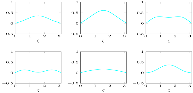
Figure 1: Galerkin solution to the stochastic damped wave equation in (6).

In Figure 1 we plot the numerical solution to the stochastic damped wave equation for $\zeta\in[0,\pi]$ and in the time interval $[0,\pi]$ where we set $\alpha=2$, $n=1000$ and $m=2$ (e.g. $2$ stochastic inputs). The weighting functions for the two inputs are $f_{1}=2\exp(-(x-\pi/2)^{2})$ and $f_{2}=\sin(x)\exp(-(x-\pi/2)^{2})$. The noise processes are $M_{1}(t)=\frac{W(t)}{\sqrt{2}}$ and $M_{2}(t)=\sum_{i=1}^{N(t)}K_{i}$ is a compound Poisson process, where $(N(t))_{t\geq 0}$ is a Poisson process with parameter equal to $1$, $K_{i}\sim\mathcal{U}(-\sqrt{6},\sqrt{6})$ are independent uniformly distributed jumps and $W$ is a standard Wiener process. $M_{1}$ and $M_{2}$ are independent. The plot in Figure 1 shows a particular realisation of the solution to (6) at $6$ specific times $t\in\left\{0.9,1.2,1.7,2.1,2.46,2.93\right\}$.

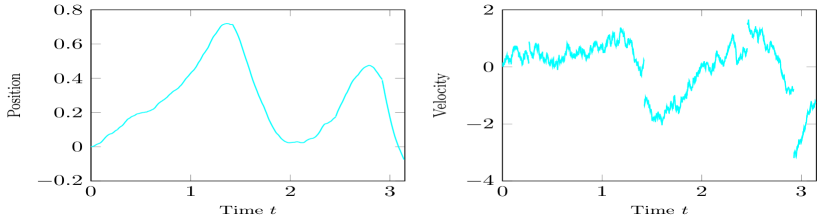
Figure 2: Components of the output (7) (position and velocity in the middle of the string) of stochastic damped wave equation in (6).

We see that the string moves up and down as expected due to the nonzero (stochastic) input. We observe that the third snapshot is taken after a jump occured in stochastic process. The corresponding output, namely both the position and the velocity in the middle of the string, is shown in Figure 2. In the plot for the velocity the noise generated by the Lévy process can be seen. The trajectory of the velocity is impacted by Lévy noise with jumps, where the velocity (e.g. the impact by wind) is randomly increased or reduced.

Figure 3: Output of stochastic damped wave equation in (6)-(7) in the phase plane.

The trajectory for the position of the cable in Figure 2 is smoother as it is the integral of the velocity. Finally, Figure 3 shows the velocity versus the position of the string, for the same sample path, in a phase portrait. The four jumps are clearly visible.

4 Numerical examples for MOR

We consider the spectral Galerkin discretisation of the second order damped wave equation which we discussed in detail in Section 3, and in particular, the example in (6)-(7) with two stochastic inputs and two outputs, namely position and velocity of the middle of the string. We set $\alpha=2$ and choose the weighting functions $f_{i}$ and the noise processes $M_{i}$ ($i=1,2$) as in Figure 1. We fix the state dimension to $n=1000$ and reduce the Galerkin solution by BT and SPA. For computing the trajectories of the SDE we use the Euler-Maruyama method (see, e.g. [14, 15]).

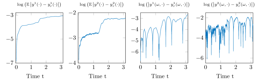
Figure 4: Logarithmic errors of BT for position $y^{1}$ and velocity $y^{2}$ with $r=6$.

Figures 4 and 5 show the logarithmic errors for the position $y^{1}$ and the velocity $y^{2}$ of the middle of the string, if MOR by BT is applied to the wave equation with stochastic inputs when reduced models of dimension $6$ and $24$, respectively, are computed.

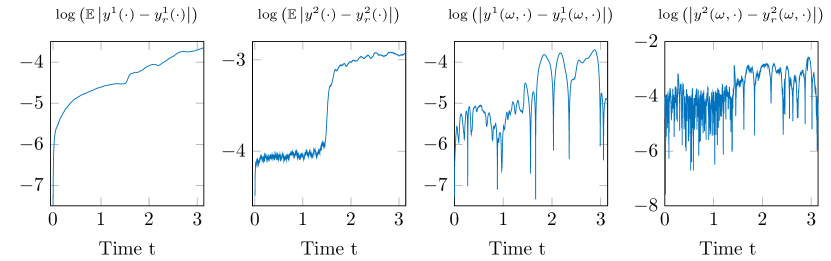
Figure 5: Logarithmic errors of BT for position $y^{1}$ and velocity $y^{2}$ with $r=24$.

The first two plots in each of the figures show the logarithmic mean error for both the position and the velocity. One observation is that the position is generally more accurate than the velocity (about one order of magnitude here), since the trajectories are smoother. Moreover, comparing the expected values of the errors of the reduced model of dimension $r=6$ (first two plots in Figure 4) with the one of dimension $r=24$ (first two plots in Figure 5) it can be seen that the latter ones are more accurate (an improvement of about one order of magnitude) as one would expect. The last two plots in Figures 4 and 5 show the logarithmic errors for position and velocity for one particular trajectory, which is the same as the one for the sample we considered in Section 3.

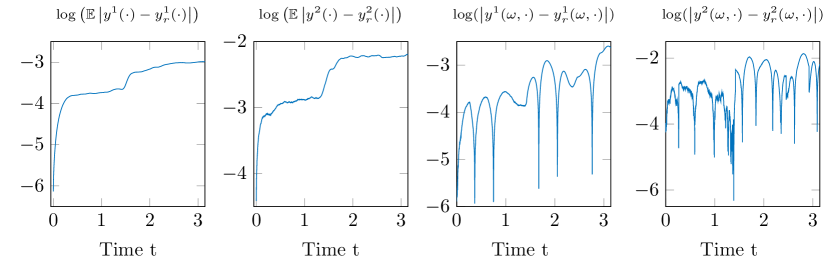
Figure 6: Logarithmic errors of SPA for position $y^{1}$ and velocity $y^{2}$ with $r=6$.

Figures 6 and 7 show the logarithmic errors for the position $y^{1}$ and the velocity $y^{2}$ of the middle of the string, if MOR by SPA is applied to the wave equation with stochastic inputs when reduced models of dimension $6$ and $24$, respectively, are computed. Again, the first two plots show the mean errors while the last two plots show the errors in particular trajectories.

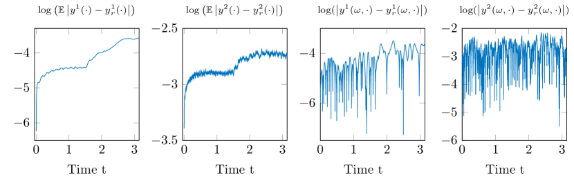
Figure 7: Logarithmic errors of SPA for position $y^{1}$ and velocity $y^{2}$ with $r=24$.

We observe that the error in the position is smaller than the error in the velocity, and, the error is smaller if a larger dimension of the reduced order model is used.

Finally, we compare the error bounds for BT (see Theorem 2.10) and SPA (see Theorem 2.11) with the worst case mean errors, that is

$$\sup_{t\in[0,\pi]}\mathbb{E}\left\|y(t)-y_{r}(t)\right\|_{\mathbb{R}^{p}}$$

for both methods in Table 1, where $y=\left(\begin{matrix}y^{1}&y^{2}\end{matrix}\right)^{T}$ is the full output of the original model and $y_{r}$ the ROM output.

Dim. ROM	Error BT	Error bound BT	Error SPA	Error bound SPA
2	7.6387e-02	9.3245e-02	1.0852e-01	1.2293e-01
4	8.5160e-03	1.2180e-02	8.6050e-03	1.2185e-02
8	5.1560e-03	9.6638e-03	5.6720e-03	9.7072e-03
16	1.8570e-03	6.6764e-03	2.4970e-03	6.7382e-03
32	6.7050e-04	4.3849e-03	1.4410e-03	4.9106e-03
64	9.9130e-05	2.3491e-03	3.1440e-04	2.6354e-03

Table 1: Error and error bounds for both BT and SPA and several dimensions of the reduced order model (ROM).

First, as expected both mean errors and error bounds are getting smaller the larger the size of the ROM. Moreover, both error bounds are rather tight and close to the actual error of the ROM, e.g. the bounds, which are worst case bounds also provide a good prediction of the true time domain error. We also note that BT performs better than SPA, both in actually computed mean errors as well as in terms of the error bounds.

5 Conclusions

We have presented theory for balancing related model order reduction (MOR) applied to linear stochastic differential equations (SDEs) with additive Lévy noise. In particular we extended the concepts of reachability and observability to stochastic systems and formulated a new reachability Gramian. We then showed how balancing related MOR which is well known for deterministic systems can be extended to SDEs with additive Lévy noise, e.g. leads to the solution of a Lyapunov equation (with a slightly different right hand side). We proved a general error bound for reduced (asymptotically stable) systems in this setting and then gave specific bounds for balanced truncation (BT) and singular perturbation approximation (SPA) which depended on the neglected (small) Hankel singular values of the linear system. We finally applied our theory to a second order damped wave equation, discretised using a spectral Galerkin method, and controlled by Lévy noise. The numerical results showed that MOR can be applied successfully and that errors for both BT and SPA are small, and the error bounds tight.

Appendix A Ito calculus

Let all stochastic processes appearing in this section be defined on a filtered probability space $\left(\Omega,\mathcal{F},(\mathcal{F}_{t})_{t\geq 0},\mathbb{P}\right)$. We denote the set of all càdlàg square integrable $\mathbb{R}$-valued martingales with respect to $(\mathcal{F}_{t})_{t\geq 0}$ by $\mathcal{M}^{2}(\mathbb{R})$.

Let $Z_{1},Z_{2}$ be scalar semimartingales. We set $\Delta Z_{i}(s):=Z_{i}(s)-Z_{i}(s-)$ with $Z_{i}(s-):=\lim_{t\uparrow s}Z_{i}(t)$ for $i=1,2$. Then the Ito product formula

$$Z_{1}(t)Z_{2}(t)=Z_{1}(0)Z_{2}(0)+\int_{0}^{t}Z_{1}(s-)dZ_{2}(s)+\int_{0}^{t}Z_{2}(s-)dZ_{1}(s)+[Z_{1},Z_{2}]_{t}$$ (105)

for $t\geq 0$ holds, see [20] or [2] for the special case of Lévy-type integrals. By [16, Theorem 4.52], the compensator process $[Z_{1},Z_{2}]$ is given by

$$[Z_{1},Z_{2}]_{t}=\left\langle M_{1}^{c},M_{2}^{c}\right\rangle_{t}+\sum_{0\leq s\leq t}\Delta Z_{1}(s)\Delta Z_{2}(s)$$ (106)

for $t\geq 0$, where $M_{1}^{c}$, $M_{2}^{c}\in\mathcal{M}^{2}(\mathbb{R})$ are the continuous martingale parts of $Z_{1}$ and $Z_{2}$ (cf. [16, Theorem 4.18]). The process $\left\langle M_{1}^{c},M_{2}^{c}\right\rangle$ is a uniquely defined angle bracket process that ensures that $M_{1}^{c}M_{2}^{c}-\left\langle M_{1}^{c},M_{2}^{c}\right\rangle$ is an $(\mathcal{F}_{t})_{t\geq 0}$- martingale, see [20, Proposition 17.2]. As a simple consequence of (105), we have:

Corollary A.1.

Let $Y$ be an $\mathbb{R}^{d}$-valued and $Z$ be an $\mathbb{R}^{n}$-valued semimartingale, then we have

$$Y(t)Z^{T}(t)=Y(0)Z^{T}(0)+\int_{0}^{t}dY(s)Z^{T}(s-)+\int_{0}^{t}Y(s-)dZ^{T}(s)+\left([Y_{i},Z_{j}]_{t}\right)_{{i=1,\ldots,d}\atop{j=1,\ldots,n}}$$

for all $t\geq 0$.

Proof.

Considering the stochastic differential of the $ij$-th component of the matrix-valued process $Y(t)Z^{T}(t)$, $t\geq 0$, and using (105) gives the result, see also [6]. ∎

Appendix B Proof of Theorem 3.3

Using $\left\|\sum_{k=1}^{q}a_{k}\right\|_{H}^{2}\leq q\sum_{k=1}^{q}\left\|a_{k}\right\|_{H}^{2}$ for $a_{k}\in H$, we obtain

$$\mathbb{E}\left\|\mathcal{X}(t)-X_{n}(t)\right\|_{H}^{2} \leq 2\mathbb{E}\left\|S(t)X_{0}-S_{n}(t)X_{0,n}\right\|_{H}^{2}$$

$$\ \ \ +2m\sum_{k=1}^{m}\mathbb{E}\left\|\int_{0}^{t}(S(t-s)\mathcal{B}_{k}-S_{n}(t-s)\mathcal{B}_{k,n})dM_{k}(s)\right\|_{H}^{2}.$$

Ito’s isometry (see e.g. [22]) yields that the right hand side can be bounded by $2\mathbb{E}\left\|S(t)X_{0}-S_{n}(t)X_{0,n}\right\|_{H}^{2}+2m\sum_{k=1}^{m}\int_{0}^{t}\left\|(S(t-s)\mathcal{B}_{k}-S_{n}(t-s)\mathcal{B}_{k,n})\right\|_{H}^{2}ds\;\mathbb{E}\left[M^{2}_{k}(1)\right]$. Since $(S(t))_{t\geq 0}$ is a contraction semigroup, we have

$$\mathbb{E}\left\|S(t)X_{0}-S_{n}(t)X_{0,n}\right\|_{H}^{2} \leq 2\mathbb{E}\left\|S(t)X_{0}-S_{n}(t)X_{0}\right\|_{H}^{2}+2\mathbb{E}\left\|S_{n}(t)X_{0}-S_{n}(t)X_{0,n}\right\|_{H}^{2}$$

$$\leq 2\mathbb{E}\left\|S(t)X_{0}-S_{n}(t)X_{0}\right\|_{H}^{2}+2\mathbb{E}\left\|X_{0}-X_{0,n}\right\|_{H}^{2}.$$ (107)

By the representation $S_{n}(t)x=\sum_{i=1}^{n}\left\langle S(t)x,h_{i}\right\rangle_{H}h_{i}$ ($x\in H$) and Lebesgue’s theorem, the bound in (107) tends to zero for $n\rightarrow\infty$. For $k\in\left\{1,\ldots,m\right\}$ we get

$$\left\|S(t-s)\mathcal{B}_{k}-S_{n}(t-s)\mathcal{B}_{k,n}\right\|_{H}^{2}$$

$$\leq 2\left\|S(t-s)\mathcal{B}_{k}-S_{n}(t-s)\mathcal{B}_{k}\right\|_{H}^{2}+2\left\|S_{n}(t-s)\mathcal{B}_{k}-S_{n}(t-s)\mathcal{B}_{k,n}\right\|_{H}^{2}$$

$$\leq 2\left\|S(t-s)\mathcal{B}_{k}-S_{n}(t-s)\mathcal{B}_{k}\right\|_{H}^{2}+2\left\|\mathcal{B}_{k}-\mathcal{B}_{k,n}\right\|_{H}^{2}$$

which tends to zero for $n\rightarrow\infty$ and hence

$$\sum_{k=1}^{m}\int_{0}^{t}\left\|(S(t-s)\mathcal{B}_{k}-S_{n}(t-s)\mathcal{B}_{k,n})\right\|_{H}^{2}ds\;\mathbb{E}\left[M^{2}_{k}(1)\right]\rightarrow 0$$

for $n\rightarrow\infty$ by Lebesgue’s theorem.

References

- [1] A. C. Antoulas. Approximation of large-scale dynamical systems. Advances in Design and Control 6. Philadelphia, PA: SIAM, 2005.
- [2] D. Applebaum. Lévy Processes and Stochastic Calculus. 2nd ed. Cambridge Studies in Advanced Mathematics 116. Cambridge: Cambridge University Press, 2009.
- [3] K. S. Arun and S. Y. Kung. Balanced approximation of stochastic systems. SIAM J. Matrix Anal. Appl., 11(1):42–68, 1990.
- [4] O. E. Barndorff-Nielsen, J. L. Jensen, and M. Sørensen. Some stationary processes in discrete and continuous time. Adv. in Appl. Probab., 30(4):989–1007, 1998.
- [5] P. Benner and T. Damm. Lyapunov equations, energy functionals, and model order reduction of bilinear and stochastic systems. SIAM J. Control Optim., 49(2):686–711, 2011.
- [6] P. Benner and M. Redmann. Model Reduction for Stochastic Systems. Stoch PDE: Anal Comp, 3(3):291–338, 2015.
- [7] R. F. Curtain. Stability of Stochastic Partial Differential Equation. J. Math. Anal. Appl., 79:352–369, 1981.
- [8] T. Damm and P. Benner. Balanced truncation for stochastic linear systems with guaranteed error bound. Proceedings of MTNS–2014, Groningen, The Netherlands, pages 1492–1497, 2014.
- [9] W. Grecksch and P. E. Kloeden. Time-discretised Galerkin approximations of parabolic stochastic PDEs. Bull. Aust. Math. Soc., 54(1):79–85, 1996.
- [10] C. Hartmann. Balanced model reduction of partially observed langevin equations: an averaging principle. Math. Comput. Model. Dyn. Syst., 17(5):463–490, 2011.
- [11] C. Hartmann, B. Schafer-Bung, and A. Thons-Zueva. Balanced averaging of bilinear systems with applications to stochastic control. SIAM Journal on Control and Optimization, 51(3):2356–2378, 2013.
- [12] C. Hartmann and C. Schütte. Balancing of partially-observed stochastic differential equations. In Decision and Control, 2008. CDC 2008. 47th IEEE Conference on, pages 4867–4872. IEEE, 2008.
- [13] E. Hausenblas. Approximation for Semilinear Stochastic Evolution Equations. Potential Anal., 18(2):141–186, 2003.
- [14] D. J. Higham and P. E. Kloeden. Numerical methods for nonlinear stochastic differential equations with jumps. Numer. Math., 101(1):101–119, 2005.
- [15] D. J. Higham and P. E. Kloeden. Strong convergence rates for backward Euler on a class of nonlinear jump-diffusion problems. J. Comput. Appl. Math., 205(2):949–956, 2007.
- [16] J. Jacod and A. N. Shiryaev. Limit Theorems for Stochastic Processes. 2nd ed. Grundlehren der Mathematischen Wissenschaften. 288. Berlin: Springer, 2003.
- [17] A. Jentzen and P. E. Kloeden. Overcoming the order barrier in the numerical approximation of stochastic partial differential equations with additive space-time noise. Proc. R. Soc. A 2009, 465:649–667, 2009.
- [18] H.-H. Kuo. Introduction to Stochastic Integration. Universitext. New York, NJ: Springer, 2006.
- [19] Y. Liu and B. D. Anderson. Singular perturbation approximation of balanced systems. Int. J. Control, 50(4):1379–1405, 1989.
- [20] M. Metivier. Semimartingales: A Course on Stochastic Processes. De Gruyter Studies in Mathematics, 2. Berlin - New York: de Gruyter, 1982.
- [21] B. C. Moore. Principal component analysis in linear systems: Controllability, observability, and model reduction. IEEE Trans. Autom. Control, 26:17–32, 1981.
- [22] S. Peszat and J. Zabczyk. Stochastic Partial Differential Equations with Lévy Noise. An evolution equation approach. Encyclopedia of Mathematics and Its Applications 113. Cambridge: Cambridge University Press, 2007.
- [23] A. J. Pritchard and J. Zabczyk. Stability and Stabilizability of Infinite-Dimensional Systems. SIAM Rev., 23:25–52, 1981.
- [24] M. Redmann. Balancing Related Model Order Reduction Applied to Linear Controlled Evolution Equations with Lévy Noise. PhD thesis, Otto-von-Guericke-Universität Magdeburg, 2016.
- [25] M. Redmann and P. Benner. Approximation and Model Order Reduction for Second Order Systems with Lévy-Noise. AIMS Proceedings, pages 945–953, 2015.
- [26] M. Redmann and P. Benner. Singular Perturbation Approximation for Linear Systems with Lévy Noise. Preprint MPIMD/15-22, Max Planck Institute Magdeburg, Dec. 2015.
- [27] K.-I. Sato and M. Yamazato. Stationary processes of Ornstein-Uhlenbeck type. Probability Theory and Mathematical Statistics, 1021(Lecture Notes in Mathematics):541–551, 2006.
- [28] W. H. Schilders, H. A. Van der Vorst, and J. Rommes. Model order reduction: theory, research aspects and applications, volume 13. Springer, 2008.
- [29] J. Zabczyk. Controllability of stochastic linear systems. Systems Control Lett., 1:25–31, 1981.