Self-calibration-based Approach to Critical Motion Sequences of
Rolling-shutter Structure from Motion

Abstract

In this paper we consider critical motion sequences (CMSs) of rolling-shutter (RS) SfM. Employing an RS camera model with linearized pure rotation, we show that the RS distortion can be approximately expressed by two internal parameters of an “imaginary” camera plus one-parameter nonlinear transformation similar to lens distortion. We then reformulate the problem as self-calibration of the imaginary camera, in which its skew and aspect ratio are unknown and varying in the image sequence. In the formulation, we derive a general representation of CMSs. We also show that our method can explain the CMS that was recently reported in the literature, and then present a new remedy to deal with the degeneracy. Our theoretical results agree well with experimental results; it explains degeneracies observed when we employ naive bundle adjustment, and how they are resolved by our method.

1 Introduction

Most consumer imaging devices such as smartphones and action cameras use CMOS sensors, the majority of which use a rolling-shutter. In recent years, increasing attention has been paid to performing SfM (structure-from-motion) from multi-view images with distortion created by a rolling shutter (RS). A number of methods have been proposed that can deal with RS distortion in several different problem settings [7, 1, 12, 6, 3]. The standard formulation is RS bundle adjustment (BA), which is to assume a model of RS distortion and optimize its model parameters together with standard camera parameters in the framework of bundle adjustment [12, 11, 24].

Despite the many studies of RS SfM, there were few studies about its degeneracy. An only exception is the recent study of Albl et al. [4]. They showed that there is a degenerate case in RS SfM and then they explained the mechanism of why it arises. However, the study only deals with a single, specific case of degeneracy. Thus, there remain several open questions, for instance, are there more degeneracy and critical cases?

A central motivation behind this study is to answer such questions. We wish to derive general representation of degeneracy in RS SfM. However, it is not a simple task, since RS SfM is a highly nonlinear problem with many unknowns. To mitigate this difficulty, in this paper, we limit our attention to a simple but practically important type of RS distortion, and then borrow the classical formulation of self-calibration of a camera, in which CMSs were previously studied extensively. To be specific, we first assume that camera motion inducing the RS distortion is pure rotation with a constant angular velocity, which may be independent of the camera pose of the viewpoint. Further assuming that the rotation is small and can be linearized, we then show that the RS distortion can be expressed by two internal parameters, specifically, skew and aspect ratio, of an imaginary camera, along with a parameter of a nonlinear transformation that is similar to (and may be regarded as a special type of) lens distortion. Assuming this model, we show that RS SfM can be recasted as self-calibration of the imaginary camera in the case where the above parameters are unknown and varying in an image sequence. In this self-calibration formulation, we will derive a general representation of critical motion sequences (CMSs). We also derive an explicitly represented CMS, which coincides with the one derived in [4], with a new remedy to deal with it. We will finally show the usefulness and effectiveness of our approach through a series of experimental results.

2 Related work

A number of studies have been conducted to deal with RS distortion in single or multi-view images. Depending on the type of problems, they are classified into absolute pose problem [1, 18, 3, 23], relative pose problem [5], multi-view optimization (bundle adjustment) [11, 12, 24], stereo [2, 22], and rectification/stabilization [6, 21, 16, 9].

The most closely related to our study is the study of Albl et al. [4]. Their study is the first to show that there is degeneracy in RS SfM. Specifically, employing the most widely used RS model with linearized rotation and constant velocity translation, they showed the existence of a CMS. The CMS is that “all images are captured by cameras with identical y (i.e., RS readout) direction in space”. They proved that these images can also be explained by RS cameras and a scene all lying in a single plane, meaning degeneracy.

Our study differs from theirs in that we derive a general representation of CMSs, although we assume an RS model of rotation-only camera motion. We also show that our method can explain the same CMS as [4] but in a different way, and then present a new method to cope with it. Another difference is that our derivation needs approximation beyond the approximation of linearized rotation. Thus, rigorously speaking, our results state that, at least in the range where our approximation is effective, RS SfM will suffer from the same degeneracy. However, considering the nature of the employed approximations, it will probably have at least instability beyond this range. These agree well with our experimental results that will be shown later.

As mentioned earlier, the central idea of our approach is to formulate the problem as self-calibration of cameras. Self-calibration of cameras was studied extensively from 1990’s to early 2000’s [19, 14, 20, 13, 15]. It had been shown that when internal camera parameters are all unknown for all images, one cannot resolve projective ambiguity emerging in reconstruction of SfM. It was then shown that if skew is zero or if at least one of the internal parameters is unknown but constant among images, projective ambiguity can be resolved and self-calibration is feasible. However, these results only guarantee that self-calibration is feasible if camera motion is general. When camera motion is a CMS, the problem can become degenerate and self-calibration is no longer feasible. As CMSs differ for different settings of self-calibration, only a few settings which are practically important were well studied [26, 17], such as when focal lengths are unknown and varying and all other parameters are known [27]. In this paper, we consider the case where skew and aspect ratio are unknown and varying and all others are known. This setting was not considered previously probably because of lack of its usefulness, and ours is the first attempt in the literature of self-calibration.

3 Modeling rolling shutter distortion

3.1 Constant motion model

Let $\mathbf{X}\equiv[X,Y,Z]^{\top}$ and $\mathbf{x}\equiv[x,y,z]^{\top}$ denote the world and camera coordinates, respectively. The coordinate transformation between these two is given by

$$\mathbf{x}=\mathtt{R}(\mathbf{X}-\mathbf{p}),$$ (1)

where $\mathtt{R}$ is a rotation matrix and $\mathbf{p}$ is a 3-vector (the world coordinates of camera position). Assuming constant camera motion during frame capture, rolling shutter (RS) distortion is modeled by

$$\begin{bmatrix}c\\ r\\ 1\end{bmatrix}\propto\mathtt{R}(r\boldsymbol{\phi})\mathtt{R}\{\mathbf{X}-(\mathbf{p}+r\mathbf{v})\},$$ (2)

where $c$ and $r$ are column ($x$) and row ($y$) coordinates, respectively; the shutter is closed in the ascending order of $r$; $\mathtt{R}(r\boldsymbol{\phi})$ and $\mathbf{v}$ represent the rotation matrix and translation vector of the camera motion; $\boldsymbol{\phi}=[\phi_{1},\phi_{2},\phi_{3}]^{\top}$ is the axis and angle representation of the rotation. Note that $\mathtt{R}$ and $\mathbf{p}$ are the camera pose when the shutter closes at $r=0$.

Assuming the angle of $\boldsymbol{\phi}$ to be small, we approximate Eq.(2) as follows:

$$\begin{bmatrix}c\\ r\\ 1\end{bmatrix}\propto(\mathtt{I}+r[\boldsymbol{\phi}]_{\times})\mathtt{R}\{\mathbf{X}-(\mathbf{p}+r\mathbf{v})\},$$ (3)

where

$$[\boldsymbol{\phi}]_{\times}=\begin{bmatrix}0&-\phi_{3}&\phi_{2}\\ \phi_{3}&0&-\phi_{1}\\ -\phi_{2}&\phi_{1}&0\end{bmatrix}.$$ (4)

This model slightly differs from previous studies (e.g., [3]) in the representation of the translational component of the camera motion during frame capture. Our model parameterizes the position of the camera in space independently of its rotation, which is physically more natural.

3.2 Rotation-only motion model

In what follows we consider the case where $\mathbf{v}$ is small and negligible. This is generally a good approximation unless a camera is close to objects in a scene. Setting $\mathbf{v}=\mathbf{0}$ and using Eq.(1) with $\mathbf{x}\equiv[x,y,z]^{\top}$, Eq.(3) can be rewritten as follows:

$$\begin{bmatrix}c\\ r\\ 1\end{bmatrix}\propto(\mathtt{I}+r[\boldsymbol{\phi}]_{\times})\begin{bmatrix}x\\ y\\ z\end{bmatrix}\propto(\mathtt{I}+r[\boldsymbol{\phi}]_{\times})\begin{bmatrix}x^{\prime}\\ y^{\prime}\\ 1\end{bmatrix},$$ (5)

where $x^{\prime}\equiv x/z$ and $y^{\prime}\equiv y/z$.

3.3 A two-step model based on affine camera approximation

Eq.(5) models the RS distortion induced by rotating a perspective camera with a constant velocity. Now, we approximate the camera with an affine camera as

$$\begin{bmatrix}c\\ r\\ 1\end{bmatrix}\propto(\mathtt{I}+r[\boldsymbol{\phi}]_{\times})\begin{bmatrix}x^{\prime}\\ y^{\prime}\\ 1\end{bmatrix}\approx\begin{bmatrix}x^{\prime}-r\phi_{3}y^{\prime}+r\phi_{2}\\ r\phi_{3}x^{\prime}+y^{\prime}-r\phi_{1}\\ 1\end{bmatrix}.$$ (6)

This model captures the “principal components” of the RS distortion, as the approximation will be accurate when $x^{\prime}$, $y^{\prime}$, and $r$ are small. This is true for image points around the principal points in the case of general cameras or for any points in the case of cameras with a telephoto lens. Note, however, that we will not use this affine camera approximation for the projection model used in SfM; regarding the projection from $(c,r)$ to image coordinates $(u,v)$, we will use a standard perspective camera model, as in Eq.(12). Thus, in the above approximation we simply neglect the effects of the second order terms of the image coordinates within the model of RS distortion. (Another proof without using this affine camera assumption is given in the supplementary material.) The validity of this approximated model will be shown experimentally in Section 5.

Eq.(6) gives a transformation $f:[x^{\prime},y^{\prime}]\mapsto[c,r]$. We show that $f$ can be approximated by a composition of two transformations.

Proposition 1.

When $\phi_{1}$, $\phi_{2}$, and $\phi_{3}$ are small, $f:[x^{\prime},y^{\prime}]\mapsto[c,r]$ can be approximated as

$$f\approx f_{p}\circ f_{d},$$ (7)

where $f_{d}:[x^{\prime},y^{\prime}]\mapsto[x^{\prime\prime},y^{\prime\prime}]$ is defined as

$$x^{\prime\prime} =x^{\prime}-\phi_{3}y^{\prime 2},$$ (8a)

$$y^{\prime\prime} =y^{\prime}+\phi_{3}x^{\prime}y^{\prime},$$ (8b)

and $f_{p}:[x^{\prime\prime},y^{\prime\prime}]\mapsto[c,r]$ as

$$\begin{bmatrix}c\\ r\\ 1\end{bmatrix}\propto\begin{bmatrix}1&\phi_{2}&0\\ 0&1-\phi_{1}&0\\ 0&0&1\end{bmatrix}\begin{bmatrix}x^{\prime\prime}\\ y^{\prime\prime}\\ 1\end{bmatrix}.$$ (9)

Proof.

We will show that the approximation (7) holds true, that is, its right hand and left hand sides are equal, in the first-order approximation with respect to $\phi_{1}$, $\phi_{2}$, and $\phi_{3}$. As for the right hand side, Substituting Eqs.(8) into Eq.(9) and neglecting the second order terms of $\phi_{1}$, $\phi_{2}$, and $\phi_{3}$, we have

$$c =x^{\prime}+\phi_{2}y^{\prime}-\phi_{3}y^{\prime 2},$$ (10a)

$$r =y^{\prime}-\phi_{1}y^{\prime}+\phi_{3}x^{\prime}y^{\prime}.$$ (10b)

As for the left hand side, substituting the second component of Eq.(6), $r=r\phi_{3}x^{\prime}+y^{\prime}-r\phi_{1}$, into the first component and then neglecting the second order terms also gives (10a). Conducting similar substitution of $r$ into $r$ itself and neglecting the second order terms yields (10b). ∎

4 Self-calibrating rolling-shutter cameras

We employ Eqs.(7)-(9) as our RS camera model. We first show that SfM based on the model is formulated as a self-calibration problem.

4.1 Problem formulation

Proposition 2.

Suppose SfM from images captured by a camera with known internal parameters. Assume the RS camera model given by Eqs.(7)-(9) with unknown motion parameters for each image. Then, the SfM problem is equivalent to self-calibration of an imaginary camera that has unknown, varying skew and aspect ratio along with varying lens distortion of a special kind.

Proof.

The first component $f_{d}$ of our two-step model $f=f_{p}\circ f_{d}$ may be interpreted as a kind of lens distortion. The most widely used model of lens distortion would be

$$x^{\prime\prime} =x^{\prime}+x^{\prime}(k_{1}\lambda^{2}+k_{2}\lambda^{4})+2p_{1}x^{\prime}y^{\prime}+p_{2}(\lambda^{2}+2x^{\prime 2})$$ (11a)

$$y^{\prime\prime} =y^{\prime}+y^{\prime}(k_{1}\lambda^{2}+k_{2}\lambda^{4})+p_{1}(\lambda^{2}+2y^{\prime 2})+2p_{2}x^{\prime}y^{\prime},$$ (11b)

where $x^{\prime}\equiv x/z$ and $y^{\prime}\equiv y/z$; $\lambda^{2}\equiv x^{\prime 2}+y^{\prime 2}$. The second terms on the right hand sides represent radial distortion and the third terms represent tangential distortion. The transformation $f_{d}$ of Eq.(8) has a similar form; there are second-order additive terms $y^{\prime 2}$ and $x^{\prime}y^{\prime}$, which appear in the tangential distortion terms.

Consider the second component $f_{p}$ of Eq.(9). The row and column coordinate $[c,r]$ are transformed to image coordinates $[u,v]$ by the matrix $\mathtt{K}$ of internal parameters as

$$\begin{bmatrix}u\\ v\\ 1\end{bmatrix}\propto\mathtt{K}\begin{bmatrix}c\\ r\\ 1\end{bmatrix}\propto\begin{bmatrix}f&0&u_{0}\\ 0&f&v_{0}\\ 0&0&1\end{bmatrix}\begin{bmatrix}c\\ r\\ 1\end{bmatrix},$$ (12)

where $f$ and $(u_{0},v_{0})$ are the focal length and the principal point of this camera. We assume here zero skew and unit aspect ratio for the sake of simplicity. The choice of other values will not change the discussions below. The substitution of Eq.(9) into the above yields

$$\begin{bmatrix}u\\ v\\ 1\end{bmatrix}\propto\begin{bmatrix}f&0&u_{0}\\ 0&f&v_{0}\\ 0&0&1\end{bmatrix}\begin{bmatrix}1&\phi_{2}&0\\ 0&1-\phi_{1}&0\\ 0&0&1\end{bmatrix}\begin{bmatrix}x^{\prime\prime}\\ y^{\prime\prime}\\ 1\end{bmatrix}\\ =\begin{bmatrix}f&\phi_{2}f&u_{0}\\ 0&(1-\phi_{1})f&v_{0}\\ 0&0&1\end{bmatrix}\begin{bmatrix}x^{\prime\prime}\\ y^{\prime\prime}\\ 1\end{bmatrix}.$$

The matrix gives an internal parameter matrix of the imaginary camera; $\phi_{1}$ (rigorously $1-\phi_{1}$) is its aspect ratio, and $\phi_{2}$ is its skew. ∎

4.2 Theory of self-calibration

Generally, self-calibration is to estimate (partially) unknown internal parameters of cameras from only images of a scene and thereby obtain metric 3D reconstruction of the scene. It was extensively studied from 1990’s to early 2000’s [19, 14, 20, 13, 15, 10]. In what follows, while summarizing these studies, we will describe how our problem can be dealt with.

4.2.1 Feasibility

If the internal parameters of cameras are all unknown, we can obtain 3D reconstruction up to projective ambiguity. It was studied previously what kind of knowledge about which internal parameters is necessary to resolve projective ambiguity. It was shown [20, 13] that it is sufficient if skew vanishes for all the images. It was also shown [15] that it suffices that only one of the five internal parameters is constant (but unknown) for all the images; others may be unknown and varying for different images. This result proves that we can indeed perform self-calibration formulated above.

Thus, theoretically, one can conduct self-calibration only if she/he has a little knowledge about internal parameters. Practically, however, this is not true because of two reasons. One is the existence of critical motion sequences (CMSs), which will be discussed later. The other is that when a large portion of internal parameters are unknown, it becomes hard to determine them with practical accuracy. Considering practical requirements, it is the most popular to assume only focal lengths [20] (and sometimes additionally principal points [17]) to be unknown and varying, and all other parameters to be known. It is interesting to point out that our case is the complete reversal in the choice of known/unknown parameters.

Additionally, simple counting argument gives a necessary condition for self-calibration. Let $m$ be the number of cameras (viewpoints), $n_{k}$ be the number of known internal parameters, and $n_{f}$ be the number of constant (but unknown) internal parameters. Then, a necessary condition is given [10] by

$$mn_{k}+(m-1)n_{f}\geq 8.$$ (13)

In our case, $n_{k}=3$ and $n_{f}=0$, from which we have $m\geq 3$ as a necessary condition.

4.2.2 Critical motion sequences

Even in cases where the above theories justify the feasibility of self-calibration, there could emerge degeneracy depending on camera poses. A set of camera poses for which the parameters cannot be uniquely determined is called a critical motion sequence (CMS).

CMSs were studied in parallel with the above studies of the feasibility of self-calibration. A catalog of CMSs for the case of constant camera parameters is shown in [26]. There are also studies for cases where some parameters are known and/or some vary. In [17], each of the cases where skew vanishes, additionally aspect ratio is known, and further additionally principal points are known are studied. In [27], a catalog of CMSs is shown for the case where focal length is unknown and varying, and others are known; this is the most popular setting of self-calibration.

However, the case considered in this paper, i.e., when skew and aspect ratio are both unknown and varying whereas all others are known, has not been considered in the literature. This may be due to lack of applications of the setting. Thus, we will examine CMSs for this case in Sec.4.3.

4.2.3 Lens distortion

When conducting self-calibration of cameras (or simply bundle adjustment), it is common to jointly estimate lens distortion (i.e., $k_{1},\ldots$ and $p_{1},\ldots$ in Eq.(11)) together with other parameters. Researchers have traditionally treated the lens distortion parameters separately from the five internal camera parameters. In fact, their uniqueness and existence have not been rigorously discussed until very recently [30]. This treatment is indeed reasonable considering nonlinear nature of the lens distortion; projective transformation maps a line onto a line, whereas lens distortion does not. In this study, adopting the same position and assuming that the parameter $\phi_{3}$ of $f_{d}$ can be treated equally to lens distortion parameters, we assume that $\phi_{3}$ can be determined uniquely independently of other parameters.

4.3 CMSs for RS camera self-calibration

We now consider CMSs for our self-calibration problem. We begin with derivation of general-purpose equations following Sec.19.2 of [10], and then tailor them for our case.

4.3.1 Equations of self-calibration

Suppose that a projective reconstruction $\{\mathtt{P}^{i},\mathbf{X}_{j}\}$ is given, where $\mathtt{P}^{i}$ is a projection matrix and $\mathbf{X}_{j}$ is a scene point. Let $\mathtt{P}^{i}=[\mathtt{A}^{i}\;|\;\mathbf{a}^{i}]$. By choosing a coordinate system we may assume that $\mathtt{A}^{1}=\mathtt{I}$ and $\mathbf{a}^{1}=\mathbf{0}$. Let $\mathtt{K}^{i}$ be the internal parameter matrix of camera $i$. The DIAC (dual image of the absolute conic) for image $i$ is given by $\omega^{*i}=\mathtt{K}^{i}\mathtt{K}^{i\top}$. A three-dimensional projective transformation $\mathtt{H}$ that transforms the projective reconstruction $\{\mathtt{P}^{i},\mathbf{X}_{j}\}$ into a metric reconstruction $\{\mathtt{P}^{i}\mathtt{H},\mathtt{H}^{-1}\mathbf{X}_{j}\}$ can be encoded as

$$\mathtt{H}=\begin{bmatrix}\mathtt{K}^{1}&\mathbf{0}\\ -\mathbf{p}^{\top}\mathtt{K}&1\end{bmatrix}.$$ (14)

Then, equations of self-calibration $(i=1,\ldots)$ are given by

$$\omega^{*i}=\left(\mathtt{A}^{i}-\mathbf{a}^{i}\mathbf{p}^{\top}\right)\omega^{*1}\left(\mathtt{A}^{i}-\mathbf{a}^{i}\mathbf{p}^{\top}\right)^{\top}.$$ (15)

Here, $\omega^{*i}$ $(i=1,\ldots)$ and $\mathbf{p}$ are unknowns. If there is knowledge about some internal parameters, it gives constraint(s) on the elements of $\omega^{*i}$.

We now derive such constraints in our case. As the principal point is known for any image, we can transform image coordinates so that it will be $(0,0)$. Then the internal parameter matrix will be

$$\mathtt{K}^{i}=\begin{bmatrix}f^{i}&s^{i}f^{i}&0\\ 0&\alpha^{i}f^{i}&0\\ 0&0&1\end{bmatrix}.$$ (16)

The DIAC will be

$$\omega^{*i}=\mathtt{K}^{i}\mathtt{K}^{i\top}=\begin{bmatrix}f^{2}+s^{2}f^{2}&s\alpha f^{2}&0\\ s\alpha f^{2}&\alpha^{2}f^{2}&0\\ 0&0&1\end{bmatrix},$$ (17)

where superscripts ($i$’s) are omitted in the matrix. From this we have constraints on the elements of the DIACs. The elimination of $s$ and $\alpha$ from the upper-left $2\times 2$ block yields

$$\omega^{*i}_{11}\omega^{*i}_{22}=\omega^{*i}_{22}f^{2}+\omega^{*i2}_{12},$$ (18a)

and the $$(1,3) (2,3)$$ and elements vanish as

$$\omega^{*i}_{13}=\omega^{*i}_{23}=0.$$ (18b)

Substituting Eq.(15) into the above equations to eliminate the elements of $\omega^{*i}$ ($i\neq 1$), we have equations that have $\omega^{*1}$ and $\mathbf{p}$ as only unknowns. Solving them for these unknowns, we can determine $\mathtt{H}$, from which we can obtain a metric reconstruction.

4.3.2 Representation of CMSs

A CMS is a set of camera poses for which the above equations becomes degenerate. Specifically, there are three equations for each camera $i$, which are obtained by substituting Eq.(15) into Eqs.(18) as described above. They differ for different cameras owing to the difference in $\mathtt{A}_{i}$ and $\mathbf{a}_{i}$. However, they can be degenerate if there is some special relation in $\{\mathtt{A}_{i},\mathbf{a}_{i}\}$ among cameras.

This analysis of degeneracy theoretically gives a complete set of CMSs. Indeed, one can check whether any given camera motion is a CMS or not. However, it is only implicitly represented, which makes intuitive understanding hard. This is also the case with other, more popular self-calibration settings such as the case of constant, unknown internal parameters [26] and the case of zero skew and known aspect ratio [17]. For such cases, researchers have derived several practically important cases. Similarly, we derive an intuitive CMS here, which coincides with the one given in [4]. Thus, the following gives yet another explanation of the CMS.

Proposition 3.

All images are captured by cameras having the parallel $y$ axis. This camera motion is a CMS. The translational components may be arbitrary.

Proof.

We denote rotation about the $y$ axis with angle $\varphi$ by $\mathtt{R}_{y}(\varphi)$. Choosing the world coordinate system, we may write the image projection of a scene point $[X,Y,Z]^{\top}$ as

$$\small\mathtt{K}\left(\mathtt{R}_{y}(\varphi)\begin{bmatrix}X\\ Y\\ Z\end{bmatrix}+\begin{bmatrix}t_{X}\\ t_{Y}\\ t_{Z}\end{bmatrix}\right)=\begin{bmatrix}f(X\cos\varphi+Z\sin\varphi+t_{X})+fs(Y+t_{Y})\\ f\alpha(Y+t_{Y})\\ -X\sin\varphi+Z\cos\varphi+t_{Z}\end{bmatrix},$$ (19)

where $\mathtt{K}$ is parameterized as in Eq.(16). It is observed that the image will not change if we multiply the $Y$ coordinate by $k$ and both $s$ and $\alpha$ by $1/k$, as $s(Y+t_{Y})=sk^{-1}\cdot k(Y+t_{Y})$ and $\alpha(Y+t_{Y})=\alpha k^{-1}\cdot k(Y+t_{Y})$. This means that we cannot determine the scale $k$ from only these images, and this camera motion is a CMS. ∎

An example of this CMS is the case where one acquires images while holding a camera horizontally with zero elevation angle. This style of capturing images is quite common. Even if a camera motion does not exactly match this CMS, if it is somewhat close to it, estimation accuracy could deteriorate depending on how close it is; see [4] for more detailed discussions.

4.3.3 A method for resolving the CMS

Besides simply avoiding it, there are several possible ways to cope with this CMS. We propose to use some method outside the framework of self-calibration to determine either $\phi_{1}$ or $\phi_{2}$ for a single camera that is selected somehow. Specifying only a single value resolves the ambiguous scale $k$ mentioned above, resolving the ambiguity of solutions. A practically easy way to do this is to find out an image $i$ in the sequence that undergoes no RS distortion (or as small distortion as possible), for which we set $\phi_{1}^{i}=0$ and/or $\phi_{2}^{i}=0$. We will show through experiments that this is indeed effective, provided that there exists such a distortion-free image in the sequence and it can be identified. Besides finding a viewpoint with $\phi_{1}^{i}=0$ or $\phi_{2}^{i}=0$, we will be able to employ various methods depending on external information available.

5 Experimental results

Our self-calibration-based formulation of RS SfM can be used not only for deriving CMSs but also for performing RS SfM in practice. To demonstrate how degeneracy arising in RS SfM can be treated by our method and also to evaluate the validity of the employed approximation of the RS model, we apply it to RS images and compare the results with the ground truths and those obtained by standard BA with/without the standard rotation-only linearized RS camera model etc.

5.1 Incorporating the RS camera model to SfM

The proposed RS model can be incorporated into bundle adjustment in the following way. The projection of a scene point $\mathbf{X}$ when our RS model is assumed is as follows: $\mathbf{X}$ is first transformed by Eq.(1) into the camera coordinates $\mathbf{x}$, and then transformed by Eqs.(8) and Eq.(4.1) in turn to yield image coordinates $[u,v]$. We assume the (genuine) internal parameters (i.e., $\mathtt{K}$ of Eq.(12)) of each camera to be known. Thus, unknowns per each camera are the six parameters of camera pose plus the three RS parameters $[\phi_{1},\phi_{2},\phi_{3}]$. Bundle adjustment is performed over these parameters for all the cameras in addition to the parameters of point cloud. We used ceres-solver [8] for implementing bundle adjustment in our experiments. The initial values of the RS parameters are set to 0, since their true values should be small due to the nature of RS distortion. The initial values of camera poses and point cloud are obtained by using these initial values for the RS parameters.

5.2 Synthetic image experiments

 

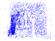
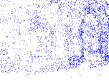
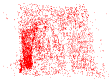
Figure 1: Example of images of points used in Experiment I. Upper: Two original images of fountain-P11. Lower: With simulated RS distortion.

We first show results using synthetic images, for which we can evaluate accuracy of 3D reconstructions using their ground truths. In the experiment, for given point cloud (scene points) and camera poses, we synthetically generate images by projecting the points onto each camera with the RS camera model (2); Fig.1 shows examples. RS distortion can generally affect every step of the SfM pipeline, i.e., matching points among images, computing initial values of camera poses as well as point cloud, and finally bundle adjustment. As the proposed method is only concerned with the last step, this experiment enables to evaluate its effectiveness independently of others.

The details are as follows. To obtain point cloud and camera poses that simulate natural scene structures and camera poses, we used Visual SFM [28, 29] to reconstruct them from real images. We used several image sequences listed in Table 1 from public datasets.

Table 1: Image sequences used for Experiment I and II.

Sequence	Dataset	# of images
fountain-P11	EPFL[25]	11
Herz-Jesu-P8	EPFL	8
castle-P19	EPFL	19
Temple	Middleburry	10(templeR0014-0023)

We then projected the reconstructed point cloud onto the images of the reconstructed cameras using the RS camera model (2). The camera motion for each image was randomly generated. For the rotation $R(r\boldsymbol{\phi})$, the axis $\boldsymbol{\phi}/\lvert\boldsymbol{\phi}\rvert$ was generated in a full sphere with a uniform distribution and the angular velocity $\lvert\boldsymbol{\phi}\rvert$ was set so that $(r_{max}-r_{min})\lvert\boldsymbol{\phi}\rvert$ equals to a random variable generated from a Gaussian distribution $N(0,\sigma_{rot}^{2})$, where $r_{max}$ and $r_{min}$ are the top and bottom rows of images. For the translation, each of its three elements was generated according to $N(0,(\sigma_{trans}\bar{t})^{2})$, where $\bar{t}$ is the average distance between consecutive camera positions in the sequence. We set $\sigma_{rot}=0.05$ radians and $\sigma_{trans}=0.05$. We used the same internal camera parameters as the original reconstruction. We added Gaussian noises $\varepsilon,\varepsilon^{\prime}\sim N(0,0.5^{2})$ to the $x$ and $y$ coordinates of each image point.

We conducted the following procedure for 100 trials for each of the image sequences listed in Table 1. In each trial, we regenerated the additive image noises and initial values for bundle adjustment. RS distortion for each image (except the first image) of each sequence was randomly generated once and fixed throughout the trials. We intentionally gave no distortion to the first image.

We applied four methods to the data thus generated. The first one is ordinary bundle adjustment without any RS camera model, which is referred to as “w/o RS.” The second and third ones are bundle adjustment incorporating the proposed RS camera model. The second one is to optimize all the RS parameters equally in bundle adjustment, which is referred to as “w/ RS.” The third one is to set $\phi_{1}^{1}=0$ and optimize all others, which is referred to as “w/ RS*”. This implements the proposed approach of resolving the CMS mentioned in Sec.4.3.3. The last one is bundle adjustment incorporating the exact RS model with linearized rotation (5), which is referred to as “w/ RS$(r[\phi]_{\times}])$”.

Figure 2 shows the results. The plots show cumulative error histograms of rotation and translation of cameras and of structure (scene points). The rotation error is measured by the average of the absolute angle of $\mathtt{R}^{i}\hat{\mathtt{R}^{i}}$ over the viewpoints, where $\mathtt{R}^{i}$ and $\hat{\mathtt{R}^{i}}$ are the true and estimated camera orientations, respectively. To eliminate scaling ambiguity for the evaluation of translation and structure, we apply a similarity transformation to them so that the camera trajectory be maximally close to the true one in the least-squares sense. Then the translation error is measured by the average of differences between the true camera position $\mathbf{p}^{i}$ and the estimated one $\hat{\mathbf{p}^{i}}$ over the viewpoints. The structure error is measured by the sum of distances between true points and their estimated counterparts.

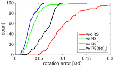
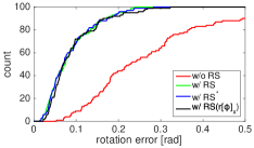
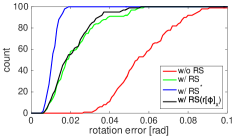
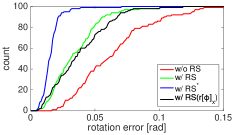
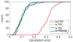
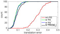
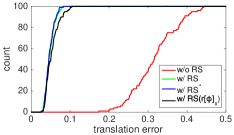
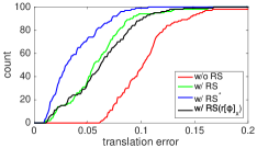
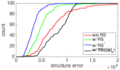
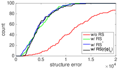
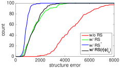
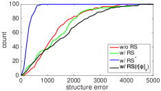
fountain-P11	Herz-Jesu-P8	castle-P19	Temple

Figure 2: Results of Experiment I. Cumulative histogram of errors of estimated rotation and translation components of camera poses and of estimated points. “w/o RS” is ordinary BA without the proposed RS camera model. “w/ RS” and “w/ RS*” are BA incorporating the proposed RS model; $\phi^{1}_{1}$ is fixed to 0 for the latter. “w/ RS$(r[\phi]_{\times}])$” is BA incorporating the original RS model (5).

Several observations can be made from Fig.2. First, it is observed that the method “w/ RS*” that fixes $\phi_{1}^{1}$ shows the best performance for all the sequences. The method “w/ RS” rivals “w/ RS*”’ only for Herz-Jesu-P8. This implies that the camera motion of fountain-P11, castle-P19, and Temple are close to CMSs, whereas that of Herz-Jesu-P8 is distant from CMSs. In fact, camera orientations in the former three sequences tend to have small elevation angles, which is one of the conditions for camera motion to be the CMS discussed in Sec.4.3.2, while those for Herz-Jesu-P8 tend to have larger elevation angles. Second, it is seen that “w/ RS$(r[\phi]_{\times}])$” (exact RS model) shows similar behaviors to “w/ RS”. This validates the approximation we used to derive our RS model (Sec.3.3), i.e., affine camera approximation and first-order approximation with respect to $(\phi_{1},\phi_{2},\phi_{3})$.

We also show typical reconstruction results for the four sequences in Figs.3-6. It is seen that for each sequence, the method “w/ RS*,” consistently yields the most accurate camera path and point cloud than others. It is also seen that the method “w/ RS” tends to yield structure that is elongated vertically, which explains the large structure error shown in the cumulative histograms of Fig.2. This structure elongation is well explained by the CMS described in Proposition 3.

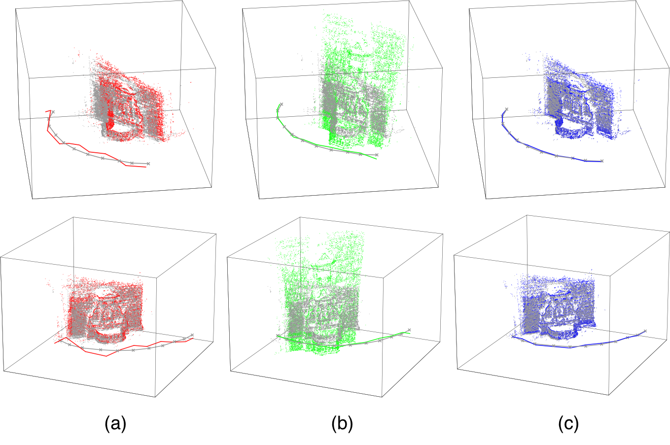
Figure 3: Typical reconstruction results for sequence fountain-P11. (a) w/o RS. (b) w/ RS. (c) w/ RS* ($\phi_{1}^{1}$ fixed). Grey dots and lines with crosses are true scene points and true camera positions, respectively.

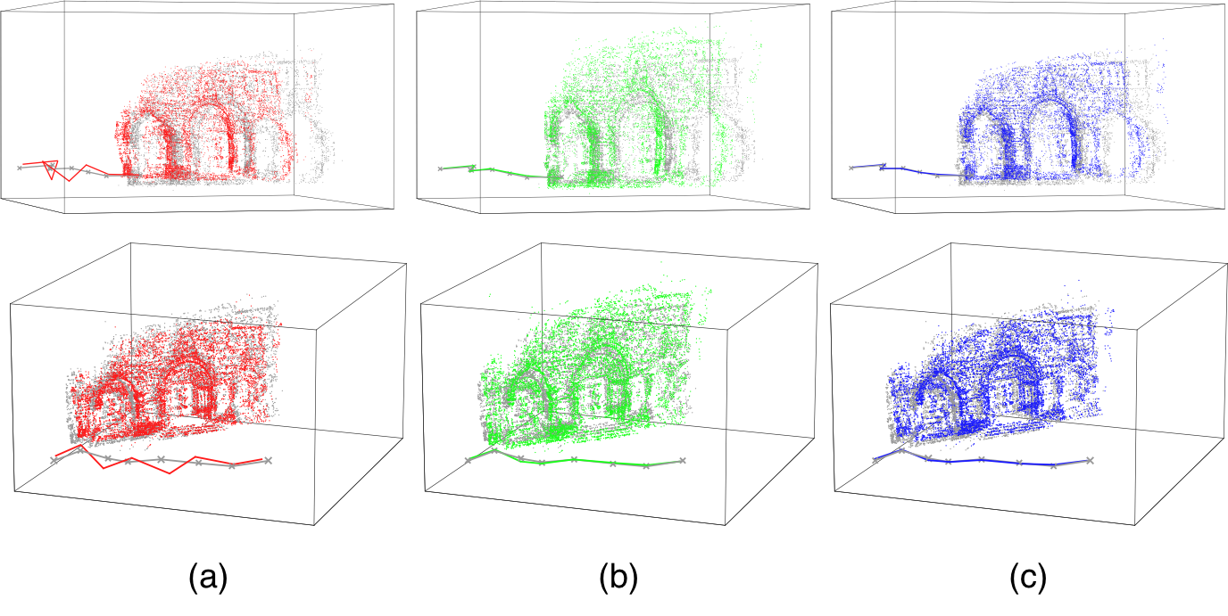
Figure 4: Typical reconstruction results for sequence Herz-Jesu-P8. (a) w/o RS. (b) w/ RS. (c) w/ RS* ($\phi_{1}^{1}$ fixed).

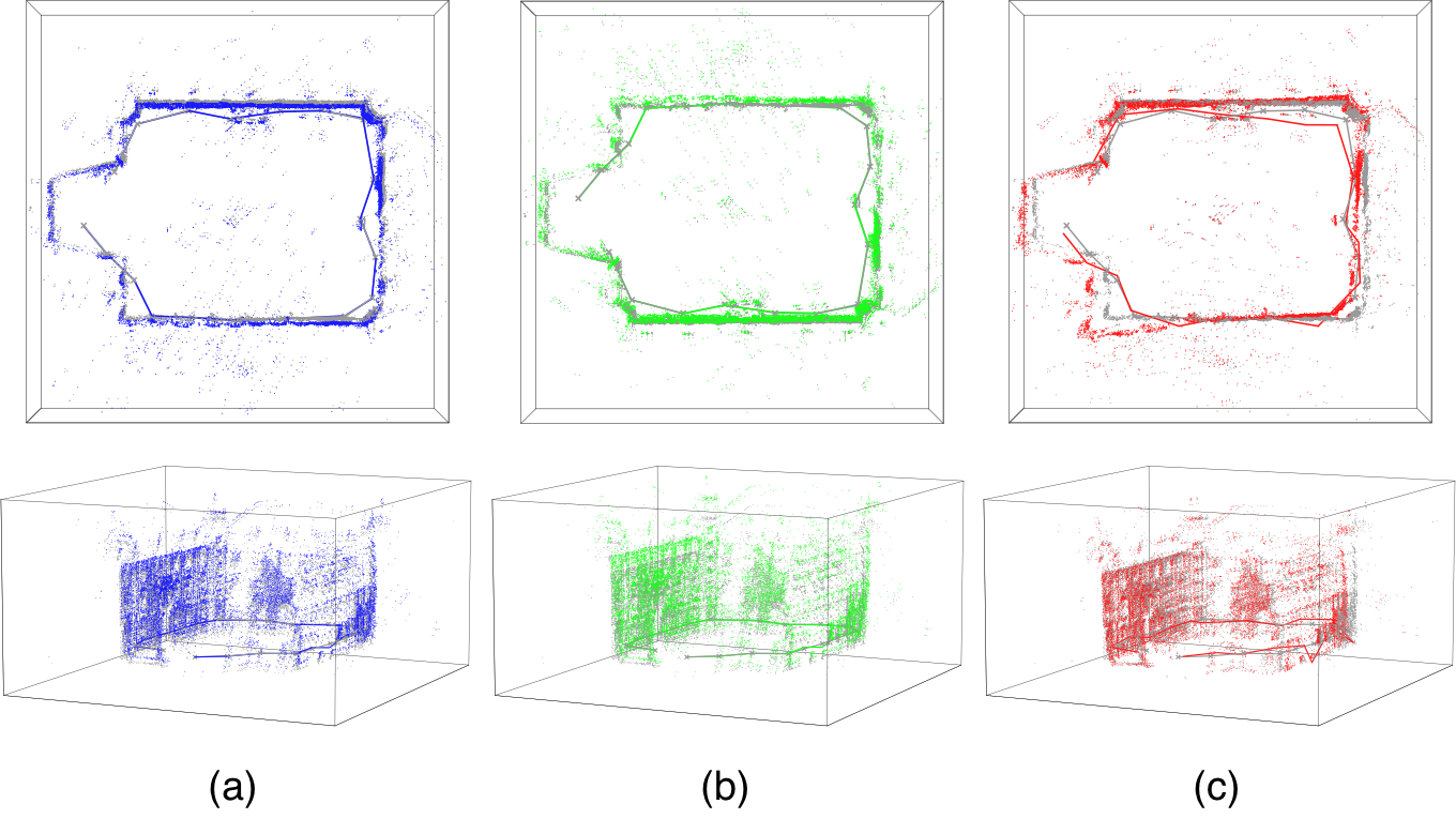
Figure 5: Typical reconstruction results for sequence castle-P19. (a) w/o RS. (b) w/ RS. (c) w/ RS* ($\phi_{1}^{1}$ fixed).

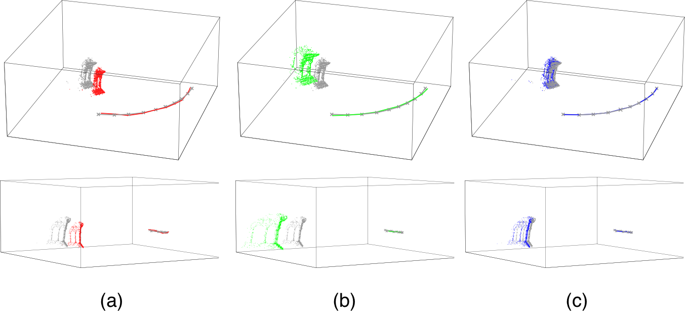
Figure 6: Typical reconstruction results for sequence Temple. (a) w/o RS. (b) w/ RS. (c) w/ RS* ($\phi_{1}^{1}$ fixed).

5.3 Real image experiments

We conducted experiments using images captured by the camera of a smartphone (iPhone 5s). We acquired still-images of a scene from a number of different viewpoints by hand-holding the smartphone. We took two images at each viewpoint, one by firmly holding the smartphone with both hands, and the other by deliberately swinging the camera a little during frame capture. As the smartphone was hand-held, its orientation cannot be precisely controlled, whereas its position should not change much between the two acquisitions; the change will be less than 20cm at each viewpoint. Each scene contains a building with the length 20-30m, and thus possible position changes will be negligibly small as compared with the building size. Thus, we use differences in the camera positions that are estimated by VisualSFM from these two image sequences as error measure. To be specific, regarding the camera positions recovered from the distortion-free sequence as the ground truth, we measure errors of those recovered from the other sequence with RS distortion. We did not prune any potentially incorrect matches. We applied two methods, one with the proposed RS model (with $\phi^{1}_{1}$ fixed assuming the first image to be distortion-free) and the other without the proposed model, and compared their accuracy. Figure 7 shows results for two different scenes Shrine1 and Shrine2. (The original images of the two scenes are shown in the supplementary material.) These results demonstrate the validity of our simplified RS model in spite of the employed approximations to derive it.

     

    

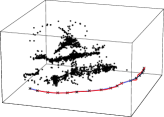
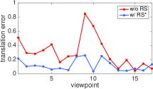
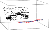
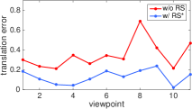
Figure 7: Two results of reconstruction from real images. The camera positions obtained from distortion-free images (assumed to be ground truths) are shown as black x marks. Those obtained by the proposed approach are in blue and those by BA without a RS model are in red. Distances from the estimated camera positions to those computed from distortion-free images.

6 Summary and conclusions

We have discussed degeneracy of rolling shutter SfM. Assuming rotation-only camera motion with linearized rotation, we have shown that, employing the affine camera approximation (i.e., the first-order approximation of the perspective effect on the RS distortion), the RS distortion can be represented by a composition of the following two transformations: i) two-dimensional projective transformation with two parameters that can be interpreted as skew and aspect ratio of an imaginary camera, and ii) one-parameter nonlinear transformation that can be interpreted as a type of lens distortion of the camera. Assuming this approximate RS camera model, we have shown that the problem can be recasted as self-calibration of the imaginary camera, in which skew and aspect ratio are unknown and varying in the image sequence. For this self-calibration problem, we have derived a general representation of CMSs, and also shown a practically important CMS that was previously reported in the literature. As ambiguity with the latter CMS can be resolved by specifying only one of the two RS distortion parameters of a single viewpoint, we have proposed to identify an image in the sequence that undergoes no distortion and set these parameters to zero. The experimental results demonstrate the effectiveness of the proposed approach to CMSs of RS SfM.

References

- [1] O. Ait-Aider, N. Andreff, J. Lavest, and P. Martinet. Simultaneous object pose and velocity computation using a single view from a rolling shutter camera. In Proc. ECCV, 2006.
- [2] O. Ait-Aider and F. Berry. Structure and kinematics triangulation with a rolling shutter stereo rig. In Proc. ICCV, 2009.
- [3] C. Albl, Z. Kukelova, and T. Pajdla. R6P-Rolling shutter absolute camera pose. In Proc. CVPR, 2015.
- [4] C. Albl, A. Sugimoto, and T. Pajdla. Degeneracies in rolling shutter sfm. In Proc. ECCV, 2016.
- [5] Y. Dai, H. Li, and L. Kneip. Rolling shutter camera relative pose: generalized epipolar geometry. In Proc. CVPR, 2016.
- [6] P. Forssén and E. Ringaby. Rectifying rolling shutter video from hand-held devices. In Proc. CVPR, 2010.
- [7] C. Geyer, M. Meingast, and S. Sastry. Geometric models of rolling-shutter cameras. In Proc. OMNIVIS, 2005.
- [8] Google Inc. Ceres Solver. http://ceres-solver.org.
- [9] M. Grundmann, V. Kwatra, and D. Castro. Calibration-free rolling shutter removal. In Proc. ICCP, 2012.
- [10] R. I. Hartley and A. Zisserman. Multiple View Geometry in Computer Vision. Cambridge University Press, ISBN: 0521540518, second edition, 2004.
- [11] J. Hedborg, P. Forssén, and M. Felsberg. Rolling shutter bundle adjustment. In Proc. CVPR, 2012.
- [12] J. Hedborg, E. Ringaby, and P. Forssén. Structure and motion estimation from rolling shutter video. In Proc. ICCV Workshops, 2011.
- [13] A. Heyden and K. Åkström. Minimal conditions on intrinsic parameters for euclidean reconstruction. In Proc. ACCV, 1998.
- [14] A. Heyden and K. Åström. Euclidean reconstruction from image sequences with varying and unknown focal length and principal point. In Proc. CVPR, 1997.
- [15] A. Heyden and K. Astrom. Flexible calibration: Minimal cases for auto-calibration. In Proc. ICCV, 1999.
- [16] C. Jia and B. Evans. Probabilistic 3-D motion estimation for rolling shutter video rectification from visual and inertial measurements. In Proc. IEEE International Workshop on Multimedia Signal Processing, 2012.
- [17] F. Kahl, B. Triggs, and K. Åström. Critical motions for auto-calibration when some intrinsic parameters can vary. Journal of Mathematical Imaging and Vision, 13:131–146, 2000.
- [18] L. Magerand, A. Bartoli, O. Ait-Aider, and D. Pizarro. Global optimization of object pose and motion from a single rolling shutter image with automatic 2d-3d matching. In Proc. ECCV, 2012.
- [19] S. J. Maybank and O. D. Faugeras. A theory of self-calibration of a moving camera. International Journal of Computer Vision, 8(2):123–151, 1992.
- [20] M. Pollefeys, R. Koch, and V. L. Gool. Self-calibration and metric reconstruction inspite of varying and unknown intrinsic camera parameters. International Journal of Computer Vision, pages 7–25, 1999.
- [21] E. Ringaby and P. Forssén. Efficient video rectification and stabilisation for cell-phones. International Journal of Computer Vision, pages 335–352, 2012.
- [22] O. Saurer, K. Koser, J. Bouguet, and M. Pollefeys. Rolling shutter stereo. In Proc. ICCV, pages 465–472, 2013.
- [23] O. Saurer, M. Pollefeys, and G. H. Lee. A minimal solution to the rolling shutter pose estimation problem. In Proc. IEEE/RSJ International Conference on Intelligent Robots and Systems, 2015.
- [24] O. Saurer, M. Pollefeys, and G. H. Lee. Sparse to dense 3d reconstruction from rolling shutter images. In Proc. CVPR, 2016.
- [25] C. Strecha, W. von Hansen, and L. Gool. On benchmarking camera calibration and multi-view stereo for high resolution imagery. In Proc. CVPR, 2008.
- [26] P. Sturm. Critical motion sequences for monocular self-calibration and uncalibrated euclidean reconstruction. In Proc. CVPR, 1997.
- [27] P. Sturm. Critical motion sequences for the self-calibration of cameras and stereo systems with variable focal length. Image and Vision Computing, 20:415–426, 2002.
- [28] C. Wu. Visual SFM. http://ccwu.me/vsfm/.
- [29] C. Wu. Towards linear-time incremental structure from motion. In Proc. 3DV, 2013.
- [30] C. Wu. Critical configurations for radial distortion self-calibration. In Proc. CVPR, 2014.