Toric Mutations in the dP2 Quiver and Subgraphs of the dP2 Brane Tiling
Abstract.
Brane tilings are infinite, bipartite, periodic, planar graphs that are dual to quivers. In this paper, we examine the del Pezzo 2 (dP2) quiver and its brane tiling, which arise from the physics literature, in terms of toric mutations on its corresponding cluster. Specifically, we give explicit formulas for all cluster variables generated by toric mutation sequences. Moreover, for each such variable, we associate a subgraph of the dP2 brane tiling to it such that its weight matches the variable.
1. Introduction
Cluster algebras are a class of commutative rings generated by cluster variables, which are partitioned into sets called clusters. Given an initial seed, an operation known as seed mutation can be applied iteratively to generate all cluster variables. The concept of cluster algebras was first introduced by Fomin and Zelevinsky [FZ02] as a tool to study total positivity and dual canonical bases in Lie theory. They have rich applications in different branches of mathematics, including algebraic combinatorics, tropical geometry, Teichmuller theory, and representation theory.
It is common to picture a cluster as a quiver with a cluster variable on each vertex. Some special quivers have planar duals, known as brane tilings, which are doubly-periodic, bipartite, planar graphs. The notion of brane tilings was first introduced in theoretical physics [FHV+06]. For such quivers, combinatorial interpretations of the cluster variables have been obtained by associating a subgraph of the brane tiling to each cluster variable such that the Laurent polynomial of the cluster variable is recoverable from a weighting scheme applied to the subgraph. See [MS10], [Mus11], and [LS13]. In particular, the quiver and brane tiling of the third del Pezzo (dP3) surface [HS12] has been studied widely by [Zha], [LMNT14], and [LM15]. In this paper, we generalize the techniques utilized in these papers and focus on the second del Pezzo (dP2) surface. Specifically, we classify all cluster variables generated by toric mutations and give combinatorial interpretations for them.
In Section 2, we start with background material on quivers and cluster mutations, and then introduce our main objects of the paper, the dP2 quiver and its corresponding brane tiling. Our contribution begins in Section 3, where we introduce -mutations (Definition 3.1) so that all toric mutations can be written in a specific form of -mutation sequences (Theorem 3.3). From there, we are able to explicitly write down the cluster variables arise from these -mutation sequences (Theorem 4.5) and classify all of them in a simple format (Corollary 4.6). In the second half of the paper, we give combinatorial interpretations for these cluster variables by associating subgraphs of the dP2 brane tiling to them, such that the “weights” of the subgraphs equal the cluster variables. Our main theorem (Theorem 6.6) provides each cluster variable with a contour, where the weighting scheme is described in Section 5 and the rules to obtain a subgraph from a contour is given in Section 6. The proof of our main theorem is shown in Section 7, which is done by induction and case work. We provide detailed description of our proof techniques and sample proofs for a few cases. The rest of the cases are proved in the same way with necessary data given in Appendix 9. We finish with a discussion regarding a similar quiver and brane tiling, which also generate the Laurent polynomials of the Somos-5 sequence, studied by David Speyer [Spe07] in Section 8.
2. Preliminaries
2.1. Quiver and Cluster Mutations
Definition 2.1 (Quiver and Cluster).
A quiver is a finite directed graph with a set of vertices and a set of edges . We can associate a cluster variable to the vertex labeled . The cluster is the ordered set of cluster variables at each vertex, assuming . For a cluster , let refer to the th cluster variable.
In this paper, we allow quivers to have multiple edges connecting two vertices but there can be no 2-cycles or 1-cycles (loops).
Definition 2.2 (Quiver Mutation).
Mutating at a vertex in is denoted by and corresponds to the following actions on the quiver:
-
•
For every 2-path through (e.g. ), add an edge from to .
-
•
Reverse the directions of the arrows incident to .
-
•
Delete any 2-cycles created from the previous two steps.
Correspondingly, the cluster variable at vertex is updated and all other cluster variables stay the same. The update follows this binomial exchange relation:
where is the new cluster variable at vertex and is the number of edges from to .
The binomial exchange relation replaces by the new cluster variable . We denote this replacement by
2.2. The Del Pezzo 2 Quiver and its Brane Tiling
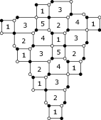
In this paper, we study a special quiver associated to the second del Pezzo surface (dP2) [BP01] and its brane tiling, as seen in Figure 1.

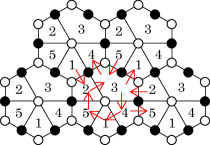
To get from a brane tiling to the corresponding quiver, we look at each edge up to translation, noticing that any brane tiling is periodic, bipartite and planar. Assume that borders block and such that as we go across from block to block , the black end point of is on the left and the white end point of is on the right. For this edge , we add an edge in the quiver that goes from to . The red arrows in Figure 1 show this process.
We use to denote the dP2 quiver and to denote its associated brane tiling .
2.3. Toric Mutation and Two Models of Quivers
Definition 2.3 (Toric Vertex and Toric Mutation).
We say that a vertex in a quiver is toric if it has in-degree 2 and out-degree 2. A toric mutation is a cluster mutation at a toric vertex.
Definition 2.4 (Model).
We say that two quivers and are of the same model if they are isomorphic as directed graphs (there exists a bijection between their vertices that preserves edges), or if is isomorphic as graph to with all edges in reversed.
It is easy to check that the dP2 quiver has two models that can be reached from the original quiver by toric mutations. Use Model 1 to denote the original quiver and Model 2 to denote the quiver obtained from by mutating at vertex 2. Figure 2 shows these two models. As a side note, the word “model” is also seen as “phase” in the literature [HS12].
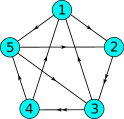

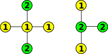
Transitions between these two models are shown in Figure 3.
3. Classification of Toric Mutation Sequences
Definition 3.1.
[-mutation sequences] We define the following operation sequences consisting of mutations and permutations, where concatenation of operations is done from left to right. A permutation permutes the vertices and their associated cluster variables accordingly.
We call each a -mutation and any concatenation of ’s a -mutation sequence.
As a side note, it is technically more correct to name “-mutation” as “-operation”. However, we follow conventions set in [LMNT14] and [LM15] and thus choose the name “-mutation”.
These -mutations all fix the quiver (but not the cluster variables), that is, , for . Notice that in the original quiver , there are no edges connecting vertex 2 and 4. This means mutation at 2 and mutation at 4 commute, so can also be written as
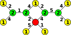
It is easy to construct Figure 4, which shows all possible toric mutation sequences that start from the original dP2 quiver and return to model 1 the first time, from Figure 3. In this way, it is clear that combinations of these seven -mutations give us all possible toric mutation sequences that start in model 1 and end in model 1 up to a permutation of vertices.
Proposition 3.2 (Relations of -mutations).
Note that it suffices to define because , , , can be written in terms of the previous three.
Theorem 3.3.
Any toric mutation sequence in dP2 quiver that starts and ends at model 1 can be written, up to a permutation of cluster variables, as , where , and
Proof.
This theorem is essentially saying that all -mutation sequences can be written in a certain form. Fix a generic -mutation sequence.
Since , we can assume that this sequence does not contain consecutive ’s and does not contain adjacent and . Therefore, we can write it as with possibly a at the beginning and a at the end, where and
Notice that by Proposition 3.2, and commute with everything. So whenever we see two consecutive ’s or consecutive ’s, we can pull them to the front. As a result, we can further simplify this sequence as with possibly a at the end, where and .
Proposition 3.2 gives , which means and “commute” with a in between. Therefore, in (with possibly a in the end), we are able to put all ’s in front of ’s. The sequence now has the form , with possibly a in the end.
Take a sufficiently large and write the sequence as . Since commute with everything, we take in the term to cancel all the ’s in , since is sufficiently large. Finally, we naturally merge the remaining ’s in the previous with , and get with possibly a in the end, with and , as desired. ∎
Remark 3.4.
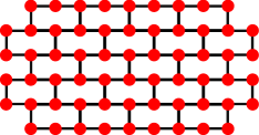
Figure 5 gives a way to visualize the -mutation sequences as an analog of alcove walk discussed in the dP3 case [LM15]. In Figure 5, each vertex corresponds to a cluster with a model 1 quiver. We can arbitrarily select one as the initial cluster. A horizontal step to the right is ; a horizontal step to the left is ; and a vertical step is .
4. Explicit Formulas for Cluster Variables
In this section, we give explicit formulas for all cluster variables that can be generated by toric mutations for the dP2 quiver.
Suppose that the cluster variables are initialized as .
Definition 4.1 (Laurent Polynomial for Somos-5 Sequence).
For , define recursively
For , define recursively
Remark 4.2.
For each , Definition 4.1 gives us a way to define as a rational function in . Moreover, the equation
| (1) |
is satisfied for each . Therefore, it is clear that if we assign 1 to , then both and give us the Somos-5 sequence.
Definition 4.3.
Define the following constants
Lemma 4.4.
For each ,
Proof.
The lemma is correct when by definition. By an inductive argument, it suffices to show that, for each ,
According to Equation (1), we have
as desired. ∎
Theorem 4.5.
Define for . Define if is even and if is odd. Then we have, for and ,
| , | |||
| , | |||
| , | |||
| , | |||
Proof.
We divide our toric mutation sequence into two steps: and . Then we use straightforward induction.
Step 1: for .
This is true for . Let us suppose that this holds for some . Then
By induction, this proves the claim for . The proof for can be done the same way.
Before doing the next step, we first show that if is odd, then
| (2) |
If is even, then is odd and these two equations become
and
which are clearly correct.
If is odd, then is even and these two equations become
and
which are clearly correct.
With the same argument, we can show that if is even, then
| (3) |
Step 2: Calculate
From step 1,
Since , no matter the parity of , when , the theorem holds. Now assume that the theorem holds for some . It suffices to show
Denote as , and let be the element of . Recall that to apply to , we first do . As we mutate vertex 2, the new cluster variable at vertex 2 is updated as
According to Lemma 4.4 and Equation (2), if is odd, the above expression becomes
Similarly by Lemma 4.4 and Equation (3), if is even, we have
Then as we mutate vertex 4, with the same argument, we can show that
So if we let , then and differ only in the and the coordinate. Specifically,
Finally, we mutate at vertex 1 in and get
After applying a permutation , we obtain the desired identity, which completes the induction step. ∎
Corollary 4.6.
All cluster variables that may appear through toric mutation sequences can be written in the forms
Proof.
We first explain that all cluster variables that appear from toric mutations can be achieved by -mutation sequences in the form of , for some and . According to Theorem 3.3, every toric mutation sequence from model 1 to model 1 can be written as or for some and . The proof for Theorem 4.5 shows that cluster variables of are included in and . Now we consider any toric mutation sequence that takes the original model 1 quiver to some model 2 quiver. According to Figure 4, this model 2 quiver can reach two different model 1 quivers in one step of toric mutation. So the cluster variables corresponding to this specific toric mutation sequence that ends on a model 2 quiver are included in the cluster variables that are generated by these two model 1 quivers.
Then we can take a closer look at the cluster variables shown in Theorem 4.5. Since depends on the value of and the parity, but not the actual value, of , it is easy to see that all cluster variables that appear can be written as for some and . Conversely, for any and , can be generated by a toric mutation sequence according to Theorem 4.5. To look at this term closely, we consider the following four cases according to the parity of and .
Case 1: is even and is even. Let and . We have . Then
Case 2: is odd and is odd. Let and . We have . Then
Case 3: is even and is odd. Let and . We have . Then
Case 4: is odd and is even. let and . We have . Then
Cases 1 and 2 can be merged by letting instead of just . Similarly cases 3 and 4 can be merged. Finally, we conclude that all cluster variables generated by toric mutations can be written as either
∎
5. Subgraphs of the Brane Tiling
For our purpose, every graph we consider is a subgraph of the dP2 brane tiling so it is bipartite, planar and weighted. For such a graph , which is bipartite, let and be its corresponding vertex sets. For any vertex set , define to be the graph obtained by removing each vertex in , as well as the edges that are incident to it, from . These notations will be used for the rest of the paper.
We want to find a subgraph for each cluster variable that appears through toric mutations, such that the subgraph’s weight equals the cluster variable. We use the weighting scheme utilized in [LM15], [LMNT14], [Spe07], [Zha], and elsewhere.
Definition 5.1 (Weight of Subgraphs).
We associate a weight to each edge bordering block labeled and . For a set of edges , define its weight to be the product of the weights of the edges. For a subgraph of the brane tiling, let be the collection of its perfect matchings where each perfect matching is represented as a set of edges. Then, we define the weight of as
In order to get recursive relations on the variables which correspond to subgraphs, we need lemmas that help us represent the weight of a large graph in terms of the weights of smaller graphs. Below we state Kuo’s condensation theorems [Kuo06], [Kuo04].
Lemma 5.2 (Balanced Kuo Condensation; Theorem 5.1 in [Kuo04]).
Let be a weighted planar bipartite graph discussed above with . Assume that are four vertices appearing in a cyclic order on a face of with and . Then
Lemma 5.3 (Unbalanced Kuo Condensation; Theorem 5.2 in [Kuo04]).
Let be a weighted planar bipartite graph discussed above with . Assume that are four vertices appearing in a cyclic order on a face of with and . Then
Lemma 5.4 (Non-alternating Kuo Condensation; Theorem 5.3 in [Kuo04]).
Let be a weighted planar bipartite graph discussed above with . Assume that are four vertices appearing in a cyclic order on a face of with and . Then
6. Contours for Cluster Variables
In this section, we describe a method to get the subgraph corresponding to any cluster variable obtained by toric mutations for the dP2 quiver. Specifically, we use 5-sided contours to cut our brane tiling. We will define the rules to cut-out the subgraphs, and the formula of the contours.
6.1. Graphs from Contours
Given a 5-tuple with and (see Figure 6 right for those relations), we consider a 5-sided contour whose side-lengths are in clockwise order, starting from the upper right corner. Figure 6 (left) shows the fundamental shape of the contour, with each length being positive. In the case of negative side-lengths, we draw the corresponding side in the opposite direction.
See Figure 7 (left) for an example of a -tuple and its contour. We abuse notation and denote a geometric contour by its corresponding -tuple.


Now we define the rule to get a subgraph from a contour.
Definition 6.1 (Rules to Get Subgraph).
The white vertex between edges and is called the special vertex.
Step 1: Given a 5-sided contour , we superimpose the contour on the brane tiling such that the vertex between side and sits on any white vertex of degree 5, while each side follows.
Step 2: On each side of positive length, we keep the black points while removing the white points; on each side of negative length, we keep the white points while removing the black points; on each side of zero length, we remove the single white point if it is not the special vertex.
Step 3: Each corner vertex is white. If the two adjacent sides of a corner vertex are both non-positive, we keep the vertex; otherwise, we remove it. As for the special vertex, if is even, we keep the special vertex; if is odd, we remove the special vertex. Call the graph that remains inside the contour .
Step 4: In the resulting graph, we connect any vertex of valence 1 to its adjacent vertex. Call the edge of this connection a forced matching. Then delete these two vertices from the graph. Repeat this step until every vertex in the subgraph has valence at least 2.
Step 5: Call the resulting graph the subgraph of contour . Often we may refer to as either or simply .
Definition 6.2.
For any graph , let denote the graph obtained by removing all forced matchings.
Remark 6.3.
Note that our notation of graphs and for a contour is the opposite of the notation in [LM15].

We have already defined the weighting of a graph in Definition 5.1. To fully recover the cluster variables from graphs, we define covering monomials for this specific brane tiling. The covering monomial has a more general definition in [JMZ00] and [Jeo11].
Definition 6.4 (Covering Monomial).
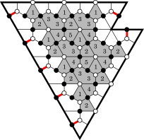
For this definition, we think of every block labeled as two separate blocks labeled . Given a contour , let be the number of blocks labeled enclosed in . Let be the number of blocks labeled adjacent to a forced matching in . If the special vertex is kept (i.e. if is even) and the contour passes through the middle of a -block near the special vertex (see Figure 8), let . Otherwise, let . The covering monomial of graph , denoted as , is the product . The covering monomial of graph , denoted as , is the product .
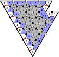
Remark 6.5.
Our definitions of weight and covering monomial remain unchanged if we think of each six sided -block as two separate four sided blocks without an edge between them. Each -block will be drawn as two separate -blocks if they appear on the boundary of our contour for sake of visualizing weight and covering monomial.
For any graph with an associated contour, denote the product of its weight and its covering monomial as
6.2. Contours of Cluster Variables
By Corollary 4.5, we have that all the cluster variables are of the form or where . Now we state the main result of this section that gives a formula of the contours of these two families.
Theorem 6.6.
For , we associate the following contours to the cluster variables such that if is the contour associated with a cluster variable, then equals the Laurent polynomial of that cluster variable.
Notice that when , we can reflect the subgraph of () along , which means we replace with and with to get the subgraph of since block 2 and block 4, and block 1 and block 5 are symmetric with respect to in the brane tiling and are also fixed if we interchange with or/and with . Therefore we only need to consider the situation where .
Before proving this result, we first look at the six possible shapes of the contours based on the relationship between and , as is shown in Figure 9.

We use the entire next section to prove the main theorem.
7. Proof of Main Theorem (Theorem 6.6)
7.1. Overview of induction procedure
We use Kuo’s condensation to inductively prove that multiplying the weight and covering monomial of these contours yields the Laurent polynomials of our cluster variables. First we show that the weights satisfy the desired recurrences. Then we show that for any form of recurrence, the covering monomials will be correct in the sense that multiplying the weight and covering monomials of our subgraphs gives the Laurent polynomial. We abuse notation by saying a graph equals a cluster variable when we mean the weight of , , will give us the cluster variable’s Laurent polynomial with the appropriate covering monomial.
The base case is , which is proved in Section 7.3. Notice that when , our formula for the contour in the main theorem contains two families: and . So essentially, there are two different cases here.
After proving the base case when , we split our way to consider the families of variables with and families of variables with separately.
For , by induction hypothesis, assume that we already have the contours for variables and for all and . Then for each , consider the following identity (recurrence):
It is clear that among all the five terms appeared above, is the only term that we do not have already. Therefore, it suffices to find some graph and points and use some version of Kuo’s condensation theorem on it to prove that this term actually equals the weight of the subgraph that we described in the main theorem, correspondingly. Note that the graph we use and the points we choose depend on some relations between and . Now that we have the terms for , consider the following identity (recurrence) for each :
Similarly, there is only one term that we do not currently have. And by some Kuo’s condensation theorem, we will get the desired result. One thing to notice here is that the above recurrence cannot be applied to since we do not have the term in our theorem. To solve this problem and get the contour formula for , we use the following recurrence:
Once this step is done, our inductive step is finished.
For , the argument is very similar. By induction hypothesis, assume that we already have the contours for variables and for all . The recurrence
will give us contours for all variables for all . After that, the recurrence
will give us contours for all variables for all . For the missing variables in the form of , we use the recurrence
This completes the inductive step.
Section 7.3 proves the base case and Section 7.4 proves one case of the inductive step. Notice that for the inductive step, we have 28 cases in total and we will not present explicit proofs for all cases. The cases are divided, generally speaking, by whether side lengths of the contour are greater or smaller than 0 and by some parity conditions on and . Section 7.2 gives a summary of the techniques used to prove the remaining cases. All of them can be proved in exactly the same format, and in Appendix 9, we provide the necessary data for readers to verify the correctness of these remaining cases.
7.2. Overview of Proof Techniques
We have different cases to prove depending on the relations between and since different relations will lead to different shapes of our contour. In this section, we introduce the general format while the details are given in Appendix 9.
Step 1. Consider a contour with the special vertex kept or removed, and 4 points inside the contour. Depending on the whether the graph is balanced or not and depending on the colors and positions of , we use a particular version of Kuo’s condensation theorems which are always of the form:
where each is a subset of . Notice that in this step, may include many forced matchings. Now we multiply both sides of the equation by , the square of the covering monomial of the graph . Each term in the equation is then of the form
Step 2. For each , we find a contour inside such that . Recall that is graph with all forced matchings removed. We find by first describing points and how removing each point separately will change the contour . Then we can add these effects together to get the total effect of removing . Notice that the additivity of such effects is nontrivial in general, but it is easy to verify for each of our cases.
This is the core step of our proof. The effects of removing each point from will be stated and justified through diagrams.
Step 3. Now we want to relate to . Consider . By definition, we know that and only differ by a set of forced matchings of inside contour and outside contour . Meanwhile, and differ by a factor of the product of all the blocks (the product of variables corresponding to the blocks) inside but outside . As each block can be in only one forced matching (otherwise the matching would not be forced), the quotient
is the product of all the blocks inside and outside that are not adjacent to any forced matchings inside and outside . Let these blocks form set . We are also using the notation with interchangeably. For each case, we will explicitly provide for a choice of points and check that
| (4) |
Also, notice that
since by definition, both and equals the product of blocks adjacent to the forced matchings of Combining these arguments, we conclude that
where
In this step, we are essentially checking that the covering monomials match up with the weights used in Kuo’s condensation theorems to give the correct Laurent polynomials.
Step 4. Using the induction hypothesis, we can identify five of the expressions as the Laurent polynomials of cluster variables. Therefore, the sixth expression is the Laurent polynomial of the next cluster variable in the sequence.
Definition 7.1 (Notation).
We establish the following notations before presenting the proof.
Let be the contour of side lengths with the special vertex kept and be the contour of side lengths with the special vertex removed. We write (resp. ) to denote the subgraph obtained from contour (resp. ). Similarly for .
We say that point is a white (or black) point on edge (or ) if it is one of the white (or black) points on the boundary of facing edge , where is some contour. This notation follows from [LM15] and it does not necessarily mean that is on edge (or ) of the contour.
7.3. Base case
When , the cluster variables and where become the terms of the Somos-5 sequence.
For , let be the contour defined in Theorem 6.6 for the initial cluster variable . We verify the weights and covering monomials of these contours. As shown in Figure 10, the subgraphs for these cluster variables are empty so they have weight . Recall that by definition, the covering monomials for and have an additional term. We can see that for .


Now assume the contours for for all give the correct Laurent polynomials for our cluster variables. We show the contour defined in Theorem 6.6 for is correct.
Case 1: . We take the following contour
Since , we have and .
Let . We then follow the steps shown in Section 7.2.
Step 1. We apply balanced Kuo’s condensation theorem (Lemma 5.2) and write down
where we let , , , , , . Then we multiply both sides by .
Step 2. We define the black points and white points as follows.
-
•
Let be any black point on edge .
-
•
Let be any white point on edge .
-
•
Let be any black point on edge .
-
•
Let be a white point near edge defined as follows:
-
–
If (mod 2), then (mod 2) so the special vertex is kept. Let be the kept special white point between edges and .
-
–
If (mod 2), then (mod 2) so the special vertex is removed. Let be the other white point on the 5-block which contains the removed white point between edges and .
-
–
We also give the effects of removing each point separately:
-
•
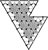
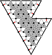
The effect of removing is We may also write this succinctly as This effect is equivalent to deleting a trapezoid along edge of the original contour.
-
•
The effect of removing is . It is equivalent to deleting a trapezoid along edge .
-
•
The effect of removing is
-
•
The effect of removing is and depending on the parity of .
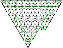
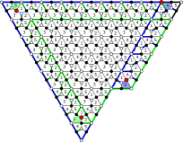
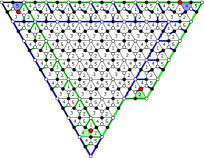
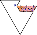
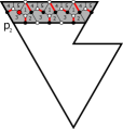
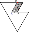
The position of each point and the effect of removing each point can be seen in Figure 11 (special point kept) and Figure 12 (special point removed). In the figures, we use big red dots to indicate point and red edges to indicate forced matchings. The shadowed region is what’s removed from the original contour after deleting the corresponding point. We also use black letters to indicate whether the special point is kept or removed in the original contour and use blue letters for the new contour.


Below, we explicitly write down the contour satisfying for each , with the corresponding cluster variable, followed from induction hypothesis. Here, we omit the details of doing explicit calculation of adding and subtracting 1’s.
Subcase 1: is even, i.e. (mod 4). We have .
Subcase 2: is odd, i.e. (mod 4). We have .
By the Somos-5 recurrence we conclude that is the graph of (after verifying step 3).
Step 3. Now that we have all of the contours , we specify the sets (defined in Section 7.2) for a specific choice of .
(Special vertex kept): let be the rightmost (B) point on edge e (not in a forced matching), be the topmost (W) point on edge a (not in a forced matching), be the bottommost (B) point on edge b (in a forced matching), be the special vertex. See Figure 13.
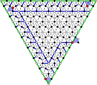
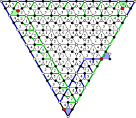
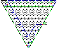
(Special vertex removed): let be the rightmost (B) point on edge e (not in a forced matching), be the topmost (W) point on edge a (not in a forced matching), be the bottommost (B) point on edge b (in a forced matching), be the other white vertex on the 5-block below the special vertex. See Figure 14.
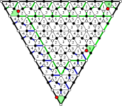
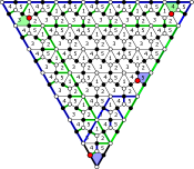
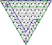
We see that equation 4 is satisfied:
Finally, we conclude that is the Laurent polynomial of , as desired.
Case 2: . Consider the following contour
Since , we have and . The proof is similar to the first case. In Step 1 we again use balanced Kuo’s condensation on and use the same notation for each . In Step 2 we define the four points as follows.
-
•
Let be any white point on edge .
-
•
Let be any black point on edge .
-
•
Let be any white point on edge .
-
•
Let be a black point near edge on edge defined as follows:
-
–
If (mod 2), then (mod 2) so the special point is kept. Let be the black point on the edge between the 4-block and 5-block above the special point.
-
–
If (mod 2), then (mod 2) so the special point is removed. Let be the lowest black point on edge .
-
–
We also give the effects of removing each point separately:
-
•
The effect of removing is .
-
•
The effect of removing is .
-
•
The effect of removing is and depending on the parity of .
-
•
The effect of removing is and depending on the parity of .
The position of each point and the effect of removing each point is shown in Figure 15 (special point kept) and Figure 16 (special point removed).


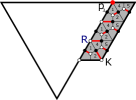


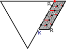

Below, we explicitly write down the contour satisfying for each , with the corresponding cluster variable (after verifying step 3).
Subcase 1: is even, i.e. (mod 4). We have .
Subcase 2: is odd, i.e. (mod 4). We have .
By the Somos-5 recurrence we conclude that is the graph of .
In Step 3 we specify the sets and verify equation 4.
(Special vertex kept): let be the bottommost (W) point on edge a (not in a forced matching), be the leftmost (B) point on edge e (not in a forced matching), be the topmost (W) point on edge d, be the (B) point on the edge between the 4-block and 5-block above the special vertex. See Figure 18.
(Special vertex removed): let be the bottommost (W) point on edge a (not in a forced matching), be the leftmost (B) point on edge e (not in a forced matching), be the topmost (W) point on edge d, be the (B) point on the edge between the 2-block and 3-block above the special vertex.
7.4. Inductive Step for , ,
As we have explained in Section 7.1, we will only show the inductive step for the case . All of the other cases can be proved in the same way and we provide the data in Appendix 9 for doing so.
Assume the contours of and , as defined in Theorem 6.6, give the correct cluster variables for any and . Now we want to show that the contour of is correct for any and .
The recurrence we use is
| (5) | ||||
| (6) |
where by the induction hypothesis, we have the correctness of the contours for cluster variables , , and .
For this case, let contour be the following:
Since , we have . Again, we use the steps described in Section 7.2. Let .
Step 1: We use non-alternating Kuo Condensation theorem (Lemma 5.4) and write down
where we let , , , , , . Then we multiply both sides by .
Step 2. We define the four points on edge respectively, where , are white, while , are black. We list the effect of each removal as follows.
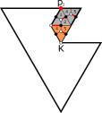
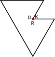
The position of these points and the effects of removing each point, when the special point is kept, is shown in Figure 19 () and Figure 20 (). Notice that after we remove , as shown in Figure 19, some area gets deleted (grey) and some area gets added (pink). The position of these points and effects of removing each point, when the special point ire removed, is shown in Figure 21.


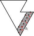
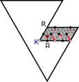
Below, we explicitly write down the contour satisfying for each , with the corresponding cluster variable, followed from induction hypothesis.
Case 1: is odd. Thus, the special vertex is kept, and .
Case 2: is even. Thus, the special vertex is removed, and .
By recurrence 5, we conclude that is the graph corresponding to .
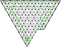
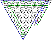
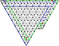
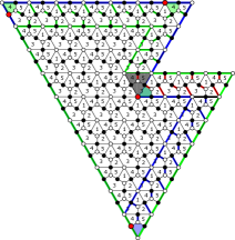
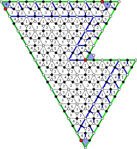
Step 3. In this step we specify the sets for a choice of and verify equation 4. In each of the diagrams in Figures 22 and 23, are the red points. Each figure shows the new contours and in green and in blue.
There is a bijection between perfect matchings of and perfect matchings of . Let be any perfect matching of . Essentially, the weight of the blocks in is exactly what we need to multiply by so that it corresponds to a term of .
We explain how Figure 22(Left) allows us to determine that the weight of is . Let us start with the green contour . A perfect matching of corresponds to a perfect matching of if we remove the red matchings and add in the green matchings. Algebraically, this corresponds to multiplying by the weight of these matchings. The covering monomial of must be multiplied by the weight of all blocks that are outside the green contour and within the largest contour . Note that the weight of these blocks are divided out by many of the green matchings and only the two 4-blocks (green) along edge e and the single 3-block (cyan) near the special vertex remain.
In this particular case, the contour is not completely contained in , so we must also divide by the weight of all blocks within and outside . Again, note that these weight of these blocks divide out all but one of the red matchings. So overall, the weight of includes from the covering monomial of , part of the weight of two green matchings (shaded), and the weight of the single red matching within (green). So the weight of is . Similarly, we find the weight of is since we simply need to multiply by the weight of blocks outside within and the only blocks that are not divided out by forced matchings are the 3-block near the special vertex (cyan) and the 3-block near (blue).
Case 1: Special vertex kept. See Figure 22.
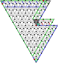
For this choice of , we have
Case 2: Special vertex removed. See Figure 23.
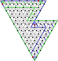
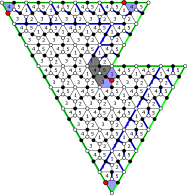
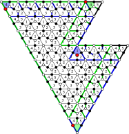
For this choice of , we have
We see that equation 4 holds in both cases.
Remark 7.2.
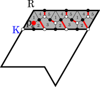
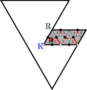
As long as we fix the side and the color of a point , the effect of removing is the same regardless of the shape of the contour, i.e. regardless of the signs of the other side lengths. For instance, as shown in Figure 24, the effects of removing in shapes and are the same.
Remark 7.3.
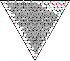
The subgraphs in dP2 quiver can look significantly different from those in dP3 quiver. When side is long, there are many forced edges, which results in different shapes. See Figure 25.
8. Comparison with the Octahedron Recurrence
David Speyer has given another combinatorial interpretation for the Laurent polynomials of the Somos-5 sequence in terms of the weight of some subgraphs of another brane tiling [Spe07]. See Figure 26 for the brane tiling and its corresponding quiver.
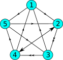
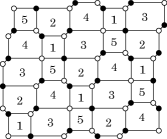
Notice that if we add a 2-cycle between vertex 2 and vertex 4 in our dP2 quiver, we will obtain the quiver shown in Figure 26. However, it is hard to describe the transformation of these two brane tilings in a simple way.


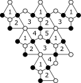
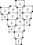
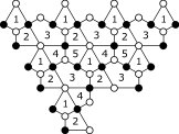
We provide a few terms of the Laurent polynomial of the Somos-5 sequence written as subgraphs of these two different brane tilings in Figure 27 and Figure 28. As we can see, the blocks in each pair of subgraphs are similar but not exactly the same. Moreover, the subgraphs corresponding to in the dP2 brane tiling are growing in two different directions (upper right and lower right) depending on the parity of . But subgraphs in the tiling considered by Speyer have a growing pattern that seems to be unrelated to the parity of . Therefore, we believe that these two problems regarding the two different tilings are sufficient different. There must exist some bijection between these subgraphs as we know how to generate them given . Also, for each pair of subgraphs, there must exist some bijection between their perfect matchings. But as these two tilings are very different despite the similarity in the corresponding quivers, we leave such a bijection as an open question for future research.


Acknowledgements
This research was carried out as part of the 2016 REU program at the School of Mathematics at University of Minnesota, Twin Cities, and was supported by NSF RTG grant DMS-1148634 and by NSF grant DMS-1351590. The authors would like to thank Sunita Chepuri and Elise DelMas for their comments and suggestions. The authors are especially grateful to Gregg Musiker for his mentorship, support, and valuable advice.
References
- [BP01] Chris E Beasley and M Ronen Plesser. Toric duality is seiberg duality. Journal of High Energy Physics, 2001(12):001, 2001.
- [EF12] Richard Eager and Sebastián Franco. Colored bps pyramid partition functions, quivers and cluster transformations. Journal of High Energy Physics, 2012(9):1–44, 2012.
- [FHV+06] Sebastián Franco, Amihay Hanany, David Vegh, Brian Wecht, and Kristian D Kennaway. Brane dimers and quiver gauge theories. Journal of High Energy Physics, 2006(01):096, 2006.
- [FZ02] Sergey Fomin and Andrei Zelevinsky. Cluster algebras i: foundations. Journal of the American Mathematical Society, 15(2):497–529, 2002.
- [HS12] Amihay Hanany and R-K Seong. Brane tilings and reflexive polygons. Fortschritte der Physik, 60(6):695–803, 2012.
- [Jeo11] In-jee Jeong. Bipartite graphs, quivers, and cluster variables. REU Report http://www. math. umn. edu/reiner/REU/Jeong2011, 2011.
- [JMZ00] I Jeong, G Musiker, and S Zhang. Brane tilings and cluster algebras i, 2000.
- [Kuo04] Eric H Kuo. Applications of graphical condensation for enumerating matchings and tilings. Theoretical Computer Science, 319(1):29–57, 2004.
- [Kuo06] Eric Kuo. Graphical condensation generalizations involving pfaffians and determinants. arXiv preprint math/0605154, 2006.
- [LM15] Tri Lai and Gregg Musiker. Beyond aztec castles: Toric cascades in the quiver. arXiv preprint arXiv:1512.00507, 2015.
- [LMNT14] Megan Leoni, Gregg Musiker, Seth Neel, and Paxton Turner. Aztec castles and the dp3 quiver. Journal of Physics A: Mathematical and Theoretical, 47(47):474011, 2014.
- [LS13] Kyungyong Lee and Ralf Schiffler. A combinatorial formula for rank 2 cluster variables. Journal of Algebraic Combinatorics, pages 1–19, 2013.
- [MS10] Gregg Musiker and Ralf Schiffler. Cluster expansion formulas and perfect matchings. Journal of Algebraic Combinatorics, 32(2):187–209, 2010.
- [Mus11] Gregg Musiker. A graph theoretic expansion formula for cluster algebras of classical type. Annals of Combinatorics, 15(1):147–184, 2011.
- [Spe07] David E Speyer. Perfect matchings and the octahedron recurrence. Journal of Algebraic Combinatorics, 25(3):309–348, 2007.
- [Zha] S Zhang. Cluster variables and perfect matchings of subgraphs of the dp3 lattice (2012). URL: http://www. math. umn. edu/~ reiner/REU/Zhang2012. pdf.
9. Appendix
Here are the data for other cases of Theorem 6.6. We group these cases by the form of cluster variables. The way to use the appendix is shown in Section 7.1 and Section 7.2.
9.1. , ,
Recurrence we use:
Kuo’s four points: are on edge respectively.
9.1.1. Case 1
Non-alternating Kuo. Shape .
(Special vertex kept): let be the topmost (W) point on edge d, be the leftmost (B) point on edge e, be the bottommost (B) point on edge b, be the special vertex.
(Special vertex removed): let be the topmost (W) point on edge d, be the leftmost (B) point on edge e, be the bottommost (B) point on edge b, be the (W) vertex bordering the 1-block below the special vertex.
9.1.2. Case 2
. Unbalanced Kuo. Shape .
When is odd, let
When is even, let
(Special vertex kept): let be the bottommost (B) point on edge d, be the leftmost (B) point on edge e, be the bottommost (B) point on edge b, be the special vertex.
(Special vertex removed): let be the bottommost (B) point on edge d, be the leftmost (B) point on edge e, be the bottommost (B) point on edge b, be the (W) vertex bordering the 1-block below the special vertex.
9.1.3. Case 3
. Balanced Kuo. Shape
When is odd, let
When is even, let
(Special vertex kept): let be the second from top (B) point on edge d, be the second from left (W) point on edge e, be the second from bottom (B) point on edge b, be the special vertex.
(Special vertex removed): let be the second from bottom (B) point on edge d, be the second from right (W) point on edge e, be the second from bottom (B) point on edge b, be the (W) vertex bordering the 1-block below the special vertex.
9.2. , ,
Recurrence we use:
Kuo’s four points: are on edge respectively.
The effect of removing and the sets used in the proof of covering monomial are the same as in Section 9.1.
9.2.1. Case 1
. Non-alternating Kuo. Shape .
9.2.2. Case 2
. Unbalanced Kuo. Shape .
When is odd, let
When is even, let
9.2.3. Case 3
. Balanced Kuo. Shape .
When is odd, let
When is even, let
9.3. , ,
Recurrence we use:
Kuo’s four points: are on edge respectively.
9.3.1. Case 1
Non-alternating Kuo. Shape .
(Special vertex kept): let be the topmost (W) point on edge d, be the topmost (W) point on edge a (not in a forced matching), be the bottommost (B) point on edge b (not in a forced matching), be the (B) point on the edge between the 4-block and 5-block above the special vertex.
(Special vertex removed): let be the topmost (W) point on edge d, be the topmost (W) point on edge a (not in a forced matching), be the bottommost (B) point on edge b (in a forced matching), be the (B) point on the edge between the 2-block and 3-block above the special vertex.
9.3.2. Case 2
Unbalanced Kuo. Shape .
(Special vertex kept): let be the topmost (W) point on edge d, be the topmost (W) point on edge a, be the bottommost (W) point on edge b, be the (B) point on the edge between the 4-block and 5-block above the special vertex.
(Special vertex removed): let be the topmost (W) point on edge d, be the topmost (W) point on edge a, be the bottommost (B) point on edge b, be the (B) point on the edge between the 2-block and 3-block above the special vertex.
9.3.3. Case 3
Balanced Kuo. Shape .
(Special vertex kept): let be the topmost (W) point on edge d, be the bottommost (B) point on edge a, be the topmost (W) point on edge b (not in a forced matching), be the (B) point on the edge between the 4-block and 5-block above the special vertex.
(Special vertex removed): let be the topmost (W) point on edge d, be the bottommost (B) point on edge a, be the topmost (W) point on edge b (not in a forced matching), be the (B) point on the edge between the 2-block and 3-block above the special vertex.
9.4. , ,
Recurrence we use:
Kuo’s four points: are on edge respectively.
The effect of removing and the sets used in the proof of covering monomial are the same as in Section 9.3.
9.4.1. Case 1
Non-alternating Kuo. Shape .
9.4.2. Case 2
Unbalanced Kuo. Shape .
9.4.3. Case 3
Balanced Kuo. Shape .
9.5. ,
Recurrence we use:
Kuo’s four points: are on edge respectively.
When : can verify the contour match the graph using Balanced Kuo or just directly verify the matching polynomial.
Let . Unbalanced Kuo. Shape .
When is odd, let
When is even, let
(Special vertex kept): let be the leftmost (W) point on edge e (the bottommost point of edge d), be the bottommost (W) point on edge a (not in a forced matching), be the special vertex, be the (B) point on the edge between the 1-block and 4-block below the special vertex.
(Special vertex removed): let be the leftmost (W) point on edge e (the bottommost point of edge d), be the bottommost (W) point on edge a (not in a forced matching), be the (W) point below the special vertex, be the (B) point below .
9.6. ,
Recurrence we use:
Kuo’s four points: are on edge respectively.
When , can check directly to see contour for is correct.
Let . Unbalanced Kuo. Shape .
When is odd, let
When is even, let
(Special vertex kept): let be the topmost (B) point on edge a (in a forced matching), be the rightmost (B) point on edge e (in a forced matching), be the (B) point with 3 neighbors on the 3-block above the special vertex, be the bottommost (W) point on edge b.
(Special vertex removed): let be the topmost (B) point on edge a (in a forced matching), be the rightmost (B) point on edge e (in a forced matching), be the (B) point on the edge between the 2-block and 3-block above the special vertex, be the bottommost (W) point on edge b.