SpatialPack: Computing the Association Between Two Spatial Processes

Abstract.

An R package SpatialPack that implements routines to compute point estimators and perform hypothesis testing of the spatial association between two stochastic sequences is introduced. These methods address the spatial association between two processes that have been observed over the same spatial locations. We briefly review the methodologies for which the routines are developed. The core routines have been implemented in C and linked to R to ensure a reasonable computational speed. Three examples are presented to illustrate the use of the package with both simulated and real data. The particular case of computing the association between two time series is also considered. Besides elementary plots and outputs we also provide a plot to visualize the spatial correlation in all directions using a new graphical tool called codispersion map. The potential extensions of SpatialPack are also discussed.

1. Introduction

The increasing need to analyze the large dimension data in spatial modeling highlights the necessity of having suitable and efficient routines to perform the spatial data analysis. For this and other reasons, researchers have been motivated to create many R packages that contain routines and functions that facilitate the computation of the standard procedures and the new theory developed in spatial statistics. Examples of commonly used packages in spatial analysis and geostatistics are geoR (Ribeiro and Diggle, 2001), spatstat (Baddeley and Turner, 2005), and GeoXp (Laurent et al., 2012), among others. A complete set of R functions developed in the context of spatial econometrics can be found in Bivand (2002).

In the analysis of spatial data, the quantification of spatial associations between two variables is an important issue, and considerable effort has been devoted to the construction of appropriate coefficients and tests for the association between two correlated variables. One can approach this issue by removing the spatial association among the observations and then applying existing techniques that have been developed for independent variables. An alternative way to manage the problem is to consider approaches that allow one to take into account the autocorrelation structure of the data.

Here, we describe a new R package SpatialPack that adds techniques to assess the spatial association between the two processes defined on a finite subset of the plane/real line. The techniques implemented in the package consist of two coefficients of association introduced by Tjøstheim and Matheron, respectively (Tjøstheim, 1978; Matheron, 1965) and one hypothesis testing procedure studied by Clifford et al. (1989). These three techniques tackle the spatial association between the two sequences defined in the same locations on the plane and are part of the standard procedures used to analyze the relationship between two spatial variables. Applications of these methodologies in several different disciplines can be found in Goovaerts (1997); Pringle and Lark (2006); Blanco-Moreno et al. (2005); Vallejos (2012) and Ojeda et al. (2012). Although these methods are part of the existing techniques to assess the spatial association between two spatial variables, they are still considered in current research (Dutilleul et al., 2008; Cuevas et al., 2013).

Tjøstheim’s coefficient is a nonparametric coefficient constructed from the ranks of suitable transformations of the coordinates for which both processes are defined. Matheron’s coefficient is also known as the codispersion coefficient and is a measurement of association that depends on a distance lag $h$. The codispersion coefficient is a normalization of the widely used cross-variogram and shares several properties with the correlation coefficient; however, the difference between the two coefficients relies on the fact that the codispersion coefficient is not centered by the process means. Instead, the coefficient quantifies the expected value of the cross-product between observations that are separated by a distance $h$. In this sense, the correlation coefficient is a crude measurement of spatial association because it does not depend on a given direction $h$ on the plane. The hypothesis testing described in Clifford et al. (1989) is based on a modified version of the correlation coefficient, which can be applied to regular or irregular grids.

Three functions were developed to compute the procedures described above: cor.spatial, codisp, and modified.ttest. All of the basic routines were built in C for efficiency and then properly linked to R. Examples with real and simulated datasets are presented to illustrate the capabilities of the techniques implemented in the package. Under specific correlation structures between and across two spatial processes, a Monte Carlo simulation study was conducted to explore the computational time as a function of the sample size. Two examples with real data are discussed to illustrate practical applications. The first example demonstrates the well-known Murray smelter site dataset in which the variables of interest are arsenic (As) and lead (Pb), both defined on a non-regular grid on the plane. The second example relates to the flammability of polymers previously studied by Rukhin and Vallejos (2008). Our analysis provides a more complete discussion about the similarity of four images used in the previous study. A brief discussion about comovement in time series, including a real data example is presented. The construction of a new graphical tool called codispersion map (Vallejos et al., 2015b) is outlined in the discussion. This map allows us to visualize the correlation between two spatial processes in all directions of interest in a single graph. Concluding remarks and possible topics for further research are also provided.

The package is available from the Comprehensive R Archive Network at http://CRAN.R-project.org/package=SpatialPack. New versions of the package, which is still under development, will be available at http://www.ies.ucv.cl/spatialpack/.

2. Methods

The methodology discussed in this section includes three different approaches to address the spatial association between two stochastic sequences indexed on a $d$-dimensional space. In all cases we consider $D\subset\mathbb{R}^{d}$, $\{X(\mbox{\boldmath$s$}):\mbox{\boldmath$s$}\in D\}$ and $\{Y(\mbox{\boldmath$s$}):\mbox{\boldmath$s$}\in D\}$ are two spatial processes and the available data at the spatial locations $\mbox{\boldmath$s$}_{1},\mbox{\boldmath$s$}_{2},\dots,\mbox{\boldmath$s$}_{n}\in D$ are the pairs $(X(\mbox{\boldmath$s$}_{i}),Y(\mbox{\boldmath$s$}_{i}))$, $i=1,2,\dots,n$. Throughout the paper we assume that $d=2$ with the exception of Example 4 in which $d=1$.

2.1. The modified correlation coefficient

Clifford et al. (1989) developed tests of association between two spatially correlated processes. These tests are based on modifying the variance and degrees of freedom of the standard $t$-test and required the estimation of the effective sample size. The later one is the factor that takes into account the spatial association of both processes. Here, we briefly described their method.

Let us consider $A\subset D$ a set of $n$ locations, say $A=\{\mbox{\boldmath$s$}_{1},\mbox{\boldmath$s$}_{2},\dots,\mbox{\boldmath$s$}_{n}\}$. Suppose that $\mbox{\boldmath$X$}=(X(\mbox{\boldmath$s$}_{1}),X(\mbox{\boldmath$s$}_{2}),\dots,X(\mbox{\boldmath$s$}_{n}))^{\top}$ and $\mbox{\boldmath$Y$}=(Y(\mbox{\boldmath$s$}_{1}),Y(\mbox{\boldmath$s$}_{2}),\dots,Y(\mbox{\boldmath$s$}_{n}))^{\top}$ are multivariate normal vectors with constant means and covariance matrices $\mbox{\boldmath$\Sigma$}_{X}$ and $\mbox{\boldmath$\Sigma$}_{Y}$, respectively.

Assume that $D$ can be divided into strata $D_{0},D_{1},D_{2},\dots$, so that $\operatorname{Cov}(X(\mbox{\boldmath$s$}_{i}),X(\mbox{\boldmath$s$}_{j}))=C_{X}(k)$ and $\operatorname{Cov}(Y(\mbox{\boldmath$s$}_{i}),Y(\mbox{\boldmath$s$}_{j}))=C_{Y}(k)$, with $\mbox{\boldmath$s$}_{i},\mbox{\boldmath$s$}_{j}\in D_{k}$, for $k=0,1,\dots$. Clifford and Richardson (1985) have suggested using

$$\widehat{C}_{Y}(h)=\sum_{\mbox{\boldmath$s$}_{i},\mbox{\boldmath$s$}_{j}\in A_{k}}(Y(\mbox{\boldmath$s$}_{i})-\overline{Y})(Y(\mbox{\boldmath$s$}_{j})-\overline{Y})/n_{k},$$

as an estimate of $C_{Y}(h)$, where $n_{k}$ is the the cardinality of $D_{k}$ and similarly for $C_{X}(k)$. Later Clifford et al. (1989) suggested to use

$$n^{-2}\sum_{h}n_{h}\widehat{C}_{X}(h)\widehat{C}_{Y}(h)$$ (2.1)

as an estimate of the conditional variance of $s_{XY}=n^{-1}\sum_{D}(X(\mbox{\boldmath$s$})-\overline{X})(Y(\mbox{\boldmath$s$})-\overline{Y})$. As a result the modified $t$-test proposed in Clifford et al. (1989) is based on the statistic

$$W=n\,s_{XY}\left(\sum_{h}n_{h}\widehat{C}_{X}(h)\widehat{C}_{Y}(h)\right)^{-2}.$$ (2.2)

Performing some approximations to the variance of the correlation coefficient $\sigma_{r}^{2}$ between processes $X(\mbox{\boldmath$s$})$ and $Y(\mbox{\boldmath$s$})$ see Appendix 1 in Clifford et al. (1989) the test statistic $W$ can be written as

$$W=(\widehat{M}-1)^{1/2}r,$$ (2.3)

where $r$ is the correlation coefficient between $X(\mbox{\boldmath$s$})$ and $Y(\mbox{\boldmath$s$})$, $\widehat{M}=1+\widehat{\sigma}^{-2}_{r}$, and

$$\widehat{\sigma}^{2}_{r}=\frac{\sum_{h}n_{h}\widehat{C}_{X}(h)\widehat{C}_{Y}(h)}{n^{2}s_{X}^{2}s_{Y}^{2}}.$$

The test statistic (2.3) was studied assuming that under the null hypothesis of no spatial correlation between processes $X(\mbox{\boldmath$s$})$ and $Y(\mbox{\boldmath$s$})$, $W$ has a $t$-student distribution with $\widehat{M}-2$ degrees of freedom. Further discussions and extensions of (2.3) can be found in Dutilleul (1993) and Dutilleul et al. (2008).

2.2. Tjøstheim’s coefficient

Tjøstheim (1978) introduced a nonparametric coefficient to measure the association between two spatial sequences. Following the notation introduced above, consider again two spatial processes $X(\mbox{\boldmath$s$})$ and $Y(\mbox{\boldmath$s$})$, defined on a two-dimensional space, that is $\mbox{\boldmath$s$}=(s_{1},s_{2})$. Define the function

$$c(u)=\begin{cases}0,&u<0,\\ 1,&u>0,\\ \frac{1}{2},&u=0.\end{cases}$$ (2.4)

Then the rank $R(\mbox{\boldmath$s$}_{i})$ of process $X(\mbox{\boldmath$s$})$ at the point $\mbox{\boldmath$s$}_{i}$ is defined as

$$R_{X}(\mbox{\boldmath$s$}_{i})=\sum_{j=1}^{n}c(X(\mbox{\boldmath$s$}_{i})-X(\mbox{\boldmath$s$}_{j})),\qquad i\neq j,$$ (2.5)

and similarly for $R_{Y}(\mbox{\boldmath$s$}_{i}).$ We define the $s_{1}$ coordinate corresponding to the rank $i$ of $X(\mbox{\boldmath$s$})$ as $F_{X}$. Then

$$F_{X}(i)=\sum_{j=1}^{n}s_{j1}\delta(i,R_{X}(\mbox{\boldmath$s$}_{i})),$$ (2.6)

where $\delta(i,j)$ is the Kronecker delta and $\mbox{\boldmath$s$}_{i}=(s_{i1},s_{i2})$, $i=1,\dots,n$. The quantities $G_{X}(i)$, $F_{Y}(i)$ and $G_{Y}(i)$ are defined similarly.

Tjøstheim’s coefficient is defined as

$$A=\frac{\sum_{i}[(F_{X}(i)-\overline{F})(F_{Y}(i)-\overline{F})][(G_{X}(i)-\overline{G})(G_{Y}(i)-\overline{G})]}{\sqrt{\sum_{i}[(F_{X}(i)-\overline{F})^{2}+(G_{X}(i)-\overline{G})^{2}]\sum_{i}[(F_{Y}(i)-\overline{F})^{2}+(G_{Y}(i)-\overline{G})^{2}]}},$$ (2.7)

where $\overline{F}=\sum_{i}F_{X}(i)/n$ and similarly for $\overline{G}$. Tjøstheim (1978) proved that if $X$ and $Y$ are two vectors of $n$ independent random variables and $\mbox{\boldmath$X$},\mbox{\boldmath$Y$}$ are also independent, then the variance of $A$ is given by

$$\operatorname{Var}(A)=\frac{(\sum_{i}s_{i1}^{2})^{2}+2(\sum_{i}s_{i1}s_{i2})^{2}+(\sum_{i}s_{i2}^{2})^{2}}{(n-1)(\sum_{i}s_{i1}^{2}+\sum_{i}s_{i2}^{2})^{2}}.$$ (2.8)

A discussion about the advantages and drawbacks of Tjøstheim’s coefficient and some extensions are in Hubert and Golledge (1982).

2.3. The codispersion coefficient

Let $X(\mbox{\boldmath$s$})$ and $Y(\mbox{\boldmath$s$})$ two intrinsically stationary processes. The cross variogram between $X(\mbox{\boldmath$s$})$ and $Y(\mbox{\boldmath$s$})$ is defined as

$$2\gamma_{XY}(\mbox{\boldmath$h$})=\operatorname{E}[(X(\mbox{\boldmath$s$}+\mbox{\boldmath$h$})-X(\mbox{\boldmath$s$}))(Y(\mbox{\boldmath$s$}+\mbox{\boldmath$h$})-Y(\mbox{\boldmath$s$}))],$$ (2.9)

for all $\mbox{\boldmath$s$},\mbox{\boldmath$s$}+\mbox{\boldmath$h$}\in D$. The codispersion coefficient studied by Matheron (1965) is a normalized version of (2.9) given by

$$\rho_{XY}(\mbox{\boldmath$h$})=\frac{\operatorname{E}[(X(\mbox{\boldmath$s$}+\mbox{\boldmath$h$})-X(\mbox{\boldmath$s$}))(Y(\mbox{\boldmath$s$}+\mbox{\boldmath$h$})-Y(\mbox{\boldmath$s$}))]}{\sqrt{\operatorname{E}[(X(\mbox{\boldmath$s$}+\mbox{\boldmath$h$})-X(\mbox{\boldmath$s$}))^{2}]\operatorname{E}[(Y(\mbox{\boldmath$s$}+\mbox{\boldmath$h$})-Y(\mbox{\boldmath$s$}))^{2}]}}=\frac{\gamma_{XY}(\mbox{\boldmath$h$})}{\sqrt{\gamma_{X}(\mbox{\boldmath$h$})\gamma_{Y}(\mbox{\boldmath$h$})}}.$$ (2.10)

A method of moment estimator of the codispersion coefficient is

$$\widehat{\rho}_{XY}(\mbox{\boldmath$h$})=\frac{\sum_{N(\mbox{\boldmath$h$})}(X(\mbox{\boldmath$s$}_{i})-X(\mbox{\boldmath$s$}_{j}))(Y(\mbox{\boldmath$s$}_{i})-Y(\mbox{\boldmath$s$}_{j}))}{[\sum_{N(\mbox{\boldmath$h$})}(X(\mbox{\boldmath$s$}_{i})-X(\mbox{\boldmath$s$}_{j}))^{2}\sum_{N(\mbox{\boldmath$h$})}(Y(\mbox{\boldmath$s$}_{i})-Y(\mbox{\boldmath$s$}_{j}))^{2}]^{1/2}},$$ (2.11)

where $N(\mbox{\boldmath$h$})=\{(\mbox{\boldmath$s$}_{i},\mbox{\boldmath$s$}_{j}):\mbox{\boldmath$s$}_{i}-\mbox{\boldmath$s$}_{j}=\mbox{\boldmath$h$},1\leq i,j\leq n\}$. Under very precise conditions the consistency and asymptotic normality of (2.11) for spatial autoregressive processes were studied by Rukhin and Vallejos Rukhin and Vallejos (2008). Vallejos Vallejos (2008) adapted the results for time series models and Ojeda et al. (2012) used the codispersion coefficient as a measure of similarity between images.

In practice the codispersion coefficient is plotted in a similar way as the correlation function in time series. Creating bins as in the variogram computation for isotropic processes (Banerjee et al., 2004), define

$$\widehat{\rho}_{XY}(h_{k})=\frac{\sum_{(\mbox{\boldmath$s$}_{i},\mbox{\boldmath$s$}_{j})\in N(h_{k})}(X(\mbox{\boldmath$s$}_{i})-X(\mbox{\boldmath$s$}_{j}))(Y(\mbox{\boldmath$s$}_{i})-Y(\mbox{\boldmath$s$}_{j}))}{[\sum_{(\mbox{\boldmath$s$}_{i},\mbox{\boldmath$s$}_{j})\in N(h_{k})}(X(\mbox{\boldmath$s$}_{i})-X(\mbox{\boldmath$s$}_{j}))^{2}\sum_{(\mbox{\boldmath$s$}_{i},\mbox{\boldmath$s$}_{j})\in N(h_{k})}(Y(\mbox{\boldmath$s$}_{i})-Y(\mbox{\boldmath$s$}_{j}))^{2}]^{1/2}},$$ (2.12)

where $N(h_{k})=\{(\mbox{\boldmath$s$}_{i},\mbox{\boldmath$s$}_{j}):\|\mbox{\boldmath$s$}_{i}-\mbox{\boldmath$s$}_{j}\|\in I_{k}\}$ for $k=1,2,\ldots,K,$ $I_{k}$ indexes the $k$th bin.

3. Software implementation in R

The code that supports the R package SpatialPack is described in this section. The set of routines correspond to the methods of quantifying the spatial association between the two processes introduced in the previous Section. In the current version of the package, three functions to compute the coefficients and tests described before are available: modified.ttest, cor.spatial and codisp. To achieve computational efficiency, each function calls a dynamic link library (shared library) written in C. Internally, some basic linear algebra subprograms (BLAS) (Lawson et al., 1979) that are included in R have been used to perform matrix operations. The routines that compute the modified $t$-test and the codispersion coefficient share a number of structures that allow the storage of intermediate results. For these routines, there is an initialization step in which the distances between the locations and the maximum distance are computed. Subsequently, the upper bounds for each bin are computed. To preserve the minimum storage requirements, we avoided storing the matrix of distances. Instead, the distances were computed directly (when they were required). This strategy facilitates the treatment of large datasets. The arguments of the implemented functions are an $n\times 2$ matrix containing the coordinates where the observations were measured and two $n$-dimensional vectors x and y that contain the observations for the first and second spatial variable, respectively. In addition, the number of classes (bins) can be specified through the argument nclass, otherwise (default) 13 classes are constructed similarly to the variog function in the geoR package (Ribeiro and Diggle, 2001). Alternatively, Sturges’ formula (Sturges, 1926) can be used to implicitly base the bin sizes on the data range.

Next, the base functions of SpatialPack are described.

3.1. Function modified.ttest

The modified $t$-test (Clifford et al., 1989), which measures the spatial association between two variables, has been computationally implemented in the function modified.ttest. To test the null hypothesis of no spatial correlation between $X(\mbox{\boldmath$s$})$ and $Y(\mbox{\boldmath$s$})$, the $F=(\widehat{M}-2)r^{2}/(1-r^{2})$ test function has been used, which (under the null hypothesis) follows an $F$ distribution with 1 and $\widehat{M}-2$ degrees of freedom. The C code underlying the function modified.ttest computes an effective sample size $\widehat{M}=1+\widehat{\sigma}_{r}^{-2}$ where $\widehat{\sigma}_{r}^{-2}$ is computed from the expression for $\sigma_{r}^{2}$ provided by Dutilleul (1993):

$$\widehat{\sigma}_{r}^{2}=\frac{\operatorname{tr}(\mbox{\boldmath$B$}\widehat{\mbox{\boldmath$\Sigma$}}_{X}\mbox{\boldmath$B$}\widehat{\mbox{\boldmath$\Sigma$}}_{Y})}{\operatorname{tr}(\mbox{\boldmath$B$}\widehat{\mbox{\boldmath$\Sigma$}}_{X})\operatorname{tr}(\mbox{\boldmath$B$}\widehat{\mbox{\boldmath$\Sigma$}}_{X})},$$

where $\mbox{\boldmath$B$}=\mbox{\boldmath$I$}_{n}-\frac{1}{n}\mbox{\boldmath$1$}_{n}\mbox{\boldmath$1$}_{n}^{\top}$ is the centering matrix of order $n$, $\mbox{\boldmath$I$}_{n}$ is the identity matrix of order $n$, and $\mbox{\boldmath$1$}_{n}$ is an $n$-dimensional vector of ones. The covariance matrices $\mbox{\boldmath$\Sigma$}_{X}$ and $\mbox{\boldmath$\Sigma$}_{Y}$ are estimated using Moran’s index (Moran, 1950). The routine does not build the matrix $B$; however, it takes advantage of its structure to simplify certain calculations. The output of the function modified.ttest is an object of the mod.ttest class, which has components that include the statistic $F$ (Fstat), the estimated degrees of freedom (dof), the $p$-value associated to the test (p.value), the upper bounds for the classes (upper.bounds), the number of observations in each class (cardinality) (card), and an $K\times 2$ matrix containing the Moran indices (imoran) for each variable under study (where $K$ is the number of classes). All of this information is appropriately displayed in the output when using the methods print and summary.

Matlab code related to the computation of the modified $t$-test (following Dutilleul’s guidelines) can be found on the website http://environmetricslab.mcgill.ca/Programs.html.

3.2. Function cor.spatial

The coefficient first introduced by Tjøstheim (1978) was implemented through the cor.spatial function. This procedure handles the possible ties that can occur in the observed values through the option ties.method = "first". This method is an existing option of function rank, which is available in R. In the computation of Tjøstheim’s coefficient, the coordinates of the ranks defined in equation (2.6) are first centered and then computed using R commands, while the computation of $A$ in equation (2.7) is performed in C. Internally, the calculations are optimized by calling level 1 routines from BLAS (Lawson et al., 1979). The procedure also returns $\operatorname{Var}(A)$ as an attribute of "variance".

3.3. Function codisp

The codisp function computes the codispersion coefficient for the general (non-rectangular) grids according to its definition in the equation (2.11). This function shares some C code developed for the function modified.ttest. The output object corresponds to a class list "codisp" whose components have a structure similar to the elements that were defined for the modified $t$-test. The value of the output coef corresponds to a vector of size nclass that contains the values of the codispersion coefficient $\widehat{\rho}_{XY}(h_{k})$ for each one of the strata previously defined. The information associated with the upper bounds of the strata is returned in card from the output subject. A generic function has been written to appropriately print the results that are obtained by the function codisp. Additionally, $\widehat{\rho}_{XY}(h_{k})$ versus $h_{k}$ can be plotted using the plot method.

4. SpatialPack in practice

In this section three examples are introduced. The first one uses simulated data to inspect the capabilities of the methods described above. The second one works with a real dataset defined on a non-rectangular grid. The third example describes a dataset that consist of four images defined on a regular grid.

4.1. Example 1: A Monte Carlo simulation study

To explore the computational time associated with the functions that compute the codispersion coefficient and the modified $t$-test, a Monte Carlo simulation experiment was conducted. Enlarged images sized $8\times 8,$ $16\times 16,$ $32\times 32,$ and $64\times 64$ were generated to study the behavior of the procedures modified.ttest and codisp as a function of the image size.

The generated images were the realizations of two correlated spatial processes. Precisely, let $X(\mbox{\boldmath$s$})$ and $Y(\mbox{\boldmath$s$})$ be two spatial processes defined for $\mbox{\boldmath$s$}\in D\subset\mathbb{Z}^{d}$. For the locations $\mbox{\boldmath$s$}_{1},\mbox{\boldmath$s$}_{2},\dots,\mbox{\boldmath$s$}_{n}$, consider the processes $\mbox{\boldmath$X$}=(X(\mbox{\boldmath$s$}_{1}),X(\mbox{\boldmath$s$}_{2}),\dots,X(\mbox{\boldmath$s$}_{n}))^{\top}$ and $\mbox{\boldmath$Y$}=(Y(\mbox{\boldmath$s$}_{1}),Y(\mbox{\boldmath$s$}_{2}),\dots,Y(\mbox{\boldmath$s$}_{n}))^{\top}$ and define the process $\mbox{\boldmath$Z$}=(\mbox{\boldmath$X$}^{\top},\mbox{\boldmath$Y$}^{\top})^{\top}\sim\mathcal{N}_{2n}(\mbox{\boldmath$0$},\mbox{\boldmath$\Sigma$}),$ where the elements of the covariance matrix $\Sigma$ are given by:

$$\mbox{\boldmath$\Sigma$}_{ij}=\begin{cases}C_{0}(\|\mbox{\boldmath$s$}_{i}-\mbox{\boldmath$s$}_{j}\|),&1\leq i,j\leq n,\\ C_{1}(\|\mbox{\boldmath$s$}_{i}-\mbox{\boldmath$s$}_{j}\|),&1\leq i\leq n,\ n+1\leq j\leq 2n,\\ C_{0}(\|\mbox{\boldmath$s$}_{i}-\mbox{\boldmath$s$}_{j}\|),&n+1\leq i,j\leq 2n,\end{cases}$$

where $C_{u}(\mbox{\boldmath$h$})=C(\mbox{\boldmath$h$},u),$ with $C(\mbox{\boldmath$h$},u)$ a nonseparable covariance function on the domain $\mathbb{R}^{d}\times\mathbb{R}$, which belongs to the parametric family (see Gelfand et al., 2011)

$$C(\mbox{\boldmath$h$},u)=\frac{1}{\psi(u^{2})^{d/2}}\,\eta\left(\frac{\|\mbox{\boldmath$h$}\|^{2}}{\psi(u^{2})}\right),$$

where $\psi(r)=(ar^{\alpha}+1)^{\beta}$, $\eta(r)=(1+(r/\sigma^{2})^{\gamma})^{-c/\gamma}$, $\alpha\in(0,1]$, $\beta\in(0,1]$, $a>0$, $c>0$, and $0<\gamma\leq 2$. In the simulation study, four images sized $8\times 8,16\times 16,32\times 32,$ and $64\times 64$ were considered. The corresponding sample sizes associated with these images are $n=8^{2},16^{2},32^{2},64^{2}$. The following set of parameters was chosen: $a=\alpha=\beta=\sigma=1$, $c=3,\gamma=2.$ The process $Z$ was generated 10 times for each image and the computational time of procedures modified.ttest and codisp was recorded. The average times for each function are shown in Figure 1.

Figure 1. computational time to evaluate the codispersion coefficient (left) and the modified t test (right) as a function of the image size (from $8\times 8$ to $64\times 64$).

We recall that each procedure requires the computation of $n(n-1)/2$ distances for each bin. Considering $\texttt{nclass}=13$, the total number of operations required to compute either codisp or modified.ttest for the two images sized $64\times 64$ is $(\texttt{nclass}+1)n(n-1)/2=117\,411\,840$. For the function modified.ttest, $n^{2}=16\,777\,216$ extra operations are needed to evaluate the test statistic. Although a number of operations are required to compute these functions, in practice the computational time remains reasonable. For example, for an image sized $64\times 64$ both procedures take approximately 5 seconds in a PC with a Core 2 quad q8400 2.66 Ghz processor, and 8 Gb RAM DDR2 800 MHz (see Figure 1). This feature is due to the strategy used to organize the computations (see description of function modified.ttest). These function types require a long computational time for large images. An application with images of size $512\times 512$ will be discussed in Example 3.

The following R function was constructed to generate the covariance function $\Sigma$. Prior to running the code we describe below, load the library SpatialPack using the R command library(SpatialPack).

⬇

Cov.nonsep <- function(h, u) {

# Constructs the nonseparable covariance function

psi <- function(r, a = 1, alpha = 1, b = 1)

(a * r^alpha + 1)^b

eta <- function(r, b = 1, g = 1, sigma = 1)

(1 + (r/sigma^2)^g)^(-b/g)

p <- 2

r <- h^2 / psi(u^2)

eta(r) / psi(u^2)^(p/2)

}

⬇

sim.images <- function(nsize, nobs = 10) {

# Simulates two correlated images

coords <- expand.grid(1:nsize, 1:nsize)

names(coords) <- c("xpos", "ypos")

dmat <- as.matrix(dist(coords, diag = TRUE, upper = TRUE))

S0 <- Cov.nonsep(dmat, u = 0)

S1 <- Cov.nonsep(dmat, u = 1)

Sigma <- rbind(cbind(S0, S1), cbind(S1, S0))

p <- ncol(Sigma)

# Generates ’nobs’ random vectors from a multivariate

# normal distribution

Z <- matrix(rnorm(nobs * p), nrow = nobs, ncol = p)

Z <- Z %*% chol(Sigma)

# Computes the codispersion coefficient

n <- nsize^2

speed <- matrix(0, nrow = nobs, ncol = 5)

for (i in 1:nobs) {

x <- Z[i,1:n]

y <- Z[i,(n+1):(2*n)]

# Replace ’codisp’ function by ’modified.ttest’ if desired

speed[i,] <- codisp(x, y, coords)$speed

}

# Creates the output

speed <- speed[,-c(4,5)]

colnames(speed) <- c("user","system","elapsed")

list(speed = speed, times = apply(speed, 2, mean))

}

4.2. Example 2: The Murray smelter site dataset

Georeferenced data have been selected for illustrative purposes here. The dataset consists of soil samples collected in and around the vacant industrially contaminated Murray smelter site (Utah, USA). This area was polluted by airborne emissions and the placement of waste slag from the smelting process. A total of 253 locations were included in the study, and soil samples were taken from each location. Each georeferenced sampling quantity is a pool composite of four closely adjacent soil samples for which the heavy metals arsenic (As) and lead (Pb) were measured. A complete description of the Murray smelter site dataset can be found in Griffith (2002) and Griffith and Paelinck (2011). The attributes As and Pb for each location are shown in Figure 2.

Figure 2. Bubble plots for As (left) and for Pb (right).

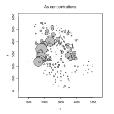
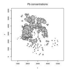
The three methods described before were used to describe the spatial association between the variables As and Pb. The R output for the code

⬇

library(SpatialPack)

x <- murray$As

y <- murray$Pb

coords <- murray[,3:4]

murray.test <- modified.ttest(x, y, coords)

murray.test

provides $F=81.9490$, the degrees of freedom 1 and 154.0617 for the numerator and denominator, respectively, of the $F$ distribution, the $p\textrm{-value}=0$ and the sample correlation coefficient $r=0.5893.$ Thus, the null hypothesis of no spatial association between the processes is rejected with a 5% level of significance. The code summary(murray.ttest) provides the upper boundaries for each of the thirteen (default) bins used in the computation of the modified $t$-test, and for each class, the Moran coefficient is also given for both variables (As and Pb).

The following R code

⬇

murray.codisp <- codisp(x, y, coords)

murray.codisp

yields the codispersion for each of the bins. These codispersion values can be plotted as a function of the lag distance in the same way as the autocorrelation function is displayed in time series. In Figure 3, $\widehat{\rho}_{XY}(h_{k})$ versus $h_{k}$ has been plotted.

Figure 3. Codispersion coefficient between As and Pb for the lag distance range from 0 to 2700 m.

The maximum value of the codispersion coefficient (0.5602) is attained for a lag distance of 1000 m.

The R code

⬇

murray.cor <- cor.spatial(x, y, coords)

murray.cor

provides Tjøstheim’s coefficient and its variance. For the Murray dataset, the value of this coefficient is $-0.1519$, and its variance is $0.0035$. This nonparametric correlation coefficient is far from the values of the other two methods, which provide evidence of positive spatial autocorrelation and a spatial codispersion in all cases larger than $0.46$. These results agree with the findings reported by Rukhin and Vallejos (2008) in a series of Monte Carlo simulations in which the correlation coefficient, Tjøstheim’s and the codispersion coefficient were compared in terms of bias and mean square error. For large values of the correlation between the processes, Tjøstheim’s coefficient was the most biased coefficient.

4.3. Example 3: Flammability of carbon nanotubes

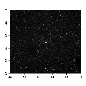
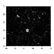
To illustrate a practical application of the codispersion coefficient with the data measured on a rectangular grid, an example related to flammability of polymers is considered here. The flame retardant property of clay polymer nanocomposites improve the physical and flammability properties of polymers (see Kashiwagi et al., 2005). The distribution of this nanotube was examined by optical microscopy. This distribution is believed to depend mainly on the distance from the top surface to the location of the polymer matrix (polymethyl methacrylate). The collected dataset consists of four $512\times 512$ images plotted in Figure 4. Images (a) and (b) were taken at the same distance from the main polymer matrix, while images (c) and (d) were both taken at the same distance from the main polymer matrix but closer than images (a) and (b). Rukhin and Vallejos (2008) used the codispersion coefficient as a metric of the closeness of the two sample polymers and fitted the spatial autoregressive processes to each image; they computed the estimated codispersion coefficient between all pairs of images. As a result, the spatial association between pairs (ac), (ad), (bc), and (bd) was almost null. However, the spatial association between the pairs (ab) and (cd) was as high (greater than 0.8) as expected. These conclusions were obtained from the codispersion coefficient $\rho_{XY}(\mbox{\boldmath$h$})$ that was evaluated in the directions $\mbox{\boldmath$h$}=(1,0)$, $\mbox{\boldmath$h$}=(0,1),$ and $\mbox{\boldmath$h$}=(1,1)$ (see Rukhin and Vallejos, 2008).

(a)

(b)

(c)

(d)

Figure 4. Dispersion of nanotubes.

Here, we used the values provided by the function codisp to generate an omnidirectional plot $\rho(\|\mbox{\boldmath$h$}\|)$ against $\|\mbox{\boldmath$h$}\|$ in the same manner that the omnidirectional variogram is plotted in spatial statistics. This process provides additional information about the codispersion range, and it is sometimes possible to analyze the shape of the codispersion curve.

Figure 5. Codispersion coefficient between the pairs of images (ab) (left) and (cd) (right).

Figure 5 shows the omnidirectional codispersion coefficient between the images pairs (ab) and (cd). In all cases, the values of the codispersion are greater than 0.88 for images (a) and (b), and greater than 0.93 for images (c) and (d), which supports the findings of Rukhin and Vallejos (2008). Additionally, the highest values of the codispersion are attained for a distance of 250 units. Figure 6 shows the codispersion for the pairs of images (ac), (ad), (bc), and (bd). In all cases, the values are close to zero.

The function takes the following computational times to compute the codispersion coefficients (considering the thirteen bins that are needed to yield the codispersion plot): (ab) 5 hours, 45 minutes and 23 seconds; (ac) 5 hours 44 minutes and 8 seconds; (ad) 5 hours 43 minutes and 53 seconds; (bc) 5 hours 40 minutes and 42 seconds; (bd) 5 hours 41 minutes and 2 seconds; (cd) 5 hours 41 minutes and 43 seconds. All computations were developed in a PC with a Core 2 quad q8400 2.66 Ghz processor, and 8 Gb RAM DDR2 800 MHz.

Figure 6. Codispersion coefficient between the pairs of images(ac) (top left), (ad) (top right), (bc) (down left), and (bd)(down right)

4.4. Example 4: Comovement between two time series

The codispersion coefficient as a measure of comovement between two time series was introduced by Vallejos (2008). This coefficient is of interest in time series to study how well two cronological sequences move together. When two spatial processes are defined on a set $D\subset\mathbb{R}^{1}$, the codispersion is called comovement coefficient. It shares a number of the standard properties of the correlation coefficient, and is interpretable as the cosine of the angle between the vectors formed by the first difference of the sample series. As in the case of the classic correlation, a comovement coefficient of $+1$ indicates that the sample function/processes being compare are rescaled/retranslated versions of one another. Similarly, a profile matched with its reflection across the time axis gives a comovement of $-1$.

SpatialPack can be used to quantify the comovement between two time series. For illustrative purposes, a real data example is presented here. The data set consist of two time series representing the monthly deaths from bronchitis, emphysema and asthma in the UK, 1974-1979. $X$ represents the males deaths while $Y$ represents the female deaths in the same period of time. The whole dataset is described in Table A.3 of Diggle (1990) and is available in R.

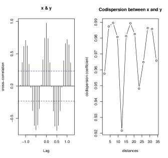
The R code

⬇

library(SpatialPack)

# UKLungDeaths from Package ’datasets’

x <- mdeaths

y <- fdeaths

coords <- cbind(1:72, rep(1,72))

z <- codisp(x, y, coords)

par(mfrow = c(1,2))

ccf(x, y, ylab = "cross-correlation", max.lag = 20)

plot(z)

produces Figure 7. There is a seasonal pattern in the cross correlation function with significant components for certain values of the lag distance $h$. The same behavior is observed for the comovement coefficient, where the maximum values are attained for $h=8$ and $h=19.$ For all values of $h$, $1\leq h\leq 35$, the comovement is greater than $0.9576$, showing a strong positive comovement between the males and females deaths in the period 1974-1979.

Figure 7. Cross-correlation function (left) and comovement coefficient (right) between series $X$ and $Y$.

5. Discussion

In this paper we have presented SpatialPack, an R package, to assess the association between two spatial processes. We provide three functions to explore the spatial association between the two sequences. The package also provides interested researchers and practitioners the facilities for working with the images and spatial datasets that are defined on non-regular grids.

The current version of SpatialPack was tested for images sized $512\times 512$ and for which the computational time is still reasonable (on average 5 hours and 40 minutes) because the computationally intensive part was written in C and the storage of the intermediate calculations was kept to a minimum.

Applications introduced illustrate how the spatial association between the two spatial sequences can be analyzed in a number of different fields and contexts including time series. Here, to emphasize that the codispersion coefficient provides information about the direction for which the highest and lowest values are attained, we show a codispersion map, a graphical display of the codispersion coefficient computed for all values of the points belonging to a grid on the plane. The codispersion map is constructed computing the method of moment estimator (2.11). As an example, for the Murray smelter site dataset discussed in Example 2, a codispersion map is shown in Figure 8 for a circular grid that considers distances up to 3000 meters (the code can be found in Vallejos et al., 2015b).

Figure 8. Codispersion map for the murray smelter site dataset of Example 2.

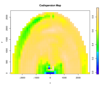
The spatial correlation that is evident for an angle of 45^∘ from Figure 2 can be observed in Figure 8 for values of the codispersion about $0.7$.

This package can be extended in several manners. For example, Cuevas et al. (2013) studied a Nadaraya-Watson estimator of the codispersion coefficient. The R function, to compute the nonparametric version of the codispersion coefficient, will be incorporated in future releases of SpatialPack including the codispersion map. On the other hand, the generalization of the codispersion coefficient to address the problem of comparing more than two spatial processes has been recently considered. In fact, Vallejos et al. (2015a) uses the $m$-dimensional spatial vector $\mbox{\boldmath$X$}=(X_{1}(\mbox{\boldmath$s$}),X_{2}(\mbox{\boldmath$s$}),\dots,X_{m}(\mbox{\boldmath$s$}))^{\top}$, where $\mbox{\boldmath$s$}\in D$. Let $X_{i}(\mbox{\boldmath$s$})$ be an intrinsically stationary process for all $l=1,2,\dots,m.$ For all $i,j=1,\dots,m$, and $\mbox{\boldmath$h$}\in D$ define

$$\gamma_{X_{i}}(\mbox{\boldmath$h$})=\operatorname{E}\left[\left(X_{i}(\mbox{\boldmath$s$}+\mbox{\boldmath$h$})-X_{i}(\mbox{\boldmath$s$})\right)^{2}\right],$$ (5.1)

and

$$\gamma_{X_{i}X_{j}}(\mbox{\boldmath$h$})=\operatorname{E}\left[\left(X_{i}(\mbox{\boldmath$s$}+\mbox{\boldmath$h$})-X_{i}(\mbox{\boldmath$s$})\right)\left(X_{j}(\mbox{\boldmath$s$}+\mbox{\boldmath$h$})-X_{j}(\mbox{\boldmath$s$})\right)\right].$$ (5.2)

The variograms and cross-variograms given in equations (5.1) and (5.2) were used to construct a codispersion matrix, called $\mbox{\boldmath$\Psi$}(\mbox{\boldmath$h$})$, containing the codispersion coefficients between the components of $X$. That is,

$$\mbox{\boldmath$\Psi$}(\mbox{\boldmath$h$})=\mbox{\boldmath$\Gamma$}_{X}^{-1/2}(\mbox{\boldmath$h$})\mbox{\boldmath$\Gamma$}_{XX}(\mbox{\boldmath$h$})\mbox{\boldmath$\Gamma$}_{X}^{-1/2}(\mbox{\boldmath$h$}),$$

where $\mbox{\boldmath$\Gamma$}_{XX}(\mbox{\boldmath$h$})=(\gamma_{X_{i}X_{j}}(\mbox{\boldmath$h$}))$ and $\mbox{\boldmath$\Gamma$}_{X}(\mbox{\boldmath$h$})=\operatorname{diag}(\gamma_{X_{i}}(\mbox{\boldmath$h$}))$. The estimation of $\mbox{\boldmath$\Psi$}(\mbox{\boldmath$h$})$ and the limiting distribution of the estimations were studied in the same way as in Rukhin and Vallejos (2008). The computational aspects and applications of the codispersion matrix will be included in future versions of SpatialPack.

Other routines related to spatial data analysis will be developed to further generalize the software. In addition, it will be of interest to develop specific methods to better the connection between SpatialPack and other packages for spatial analysis, e.g. geoR.

References

- Acosta et al. (2016) Acosta, J., Osorio, F., Vallejos, R. (2016). Effective sample size for line transect sampling models with an application to marine macroalgae. Journal of Agricultural, Biological, and Environmental Statistics 21, 407-425.
- Baddeley and Turner (2005) Baddeley, A., Turner, R. (2005). spatstat: An R package for analyzing spatial point patterns. Journal of Statistical Software 12 (6), 1-42. URL: http://www.jstatsoft.org/v12/i06/
- Banerjee et al. (2004) Banerjee, S., Carlin, B.P., Gelfand, A.E. (2004). Hierarchical Modeling and Analysis for Spatial Data. Chapman & Hall/CRC, Boca Raton.
- Bivand (2002) Bivand, R. (2002). Spatial econometrics functions in R: Classes and methods. Journal of Geographical Systems 4, 405-421.
- Blanco-Moreno et al. (2005) Blanco-Moreno, J.M., Chamorro, L., Sanz, F.X. (2005). Spatial and temporal patterns of Lolium rigidum-Avena sterellis mixed populations in a cereal field. Weed Research 46, 207-218.
- Clifford and Richardson (1985) Clifford, P., Richardson, S. (1985). Testing the association between two spatial processes. Statistics and Decisions Supp. Issue 2, 155-160.
- Clifford et al. (1989) Clifford, P., Richardson, S., Hémon, D. (1989). Assessing the significance of the correlation between two spatial processes. Biometrics 45, 123-144.
- Cuevas et al. (2013) Cuevas, F., Porcu, E., Vallejos, R. (2013). Study of spatial relationships between two sets of variables: A nonparametric approach. Journal of Nonparametric Statistics 25, 695-714.
- Diggle (1990) Diggle, P.J. (1990). Time Series: A Biostatistical Introduction. Clarendon Press, Oxford.
- Dutilleul (1993) Dutilleul, P. (1993). Modifying the t test for assessing the correlation between two spatial processes. Biometrics 49, 305-314.
- Dutilleul et al. (2008) Dutilleul, P., Pelletier, B., Alpargu, G. (2008). Modified F tests for assessing the multiple correlation between one spatial process and several others. Journal of Statistical Planning and Inference 138, 1402-1415.
- Gelfand et al. (2011) Gelfand, A.E., Diggle, P.J., Fuentes, M., Guttorp, P. (2011). Handbook of Spatial Statistics. CRC Press Taylor and Francis Group, Boca Raton.
- Goovaerts (1997) Gooaverts, P. (1997). Geostatistics for Natural Resources Evaluation. Oxford University Press, Oxford.
- Griffith (2002) Griffith, D. (2002). The geographic distribution of soil-lead concentration: Description and concerns. URISA Journal 14, 5-15.
- Griffith and Paelinck (2011) Griffith, D., Paelinck, J.H.P. (2011). Non-Stardard Spatial Statistics. Springer, New York.
- Hubert and Golledge (1982) Hubert, L., Golledge, R.G. (1982). Measuring association between spatially defined variables: Tjøstheim’s coefficient index and some extensions. Geographical Analysis 14, 273-278.
- Kashiwagi et al. (2005) Kashiwagi, T., Du, F., Winey, K.I., Groth, K.M., Shields, J.R., Bellayer, S.P., Kim, S., Douglas, J.F. (2005). Flammability properties of polymer nanocomposites with single-walled carbon nanotubes: Effects of nanotube dispersion and concentration. Polymer 46, 471-481.
- Laurent et al. (2012) Laurent, T., Ruiz-Gazen, A., Thomas-Agnan, C. (2012). GeoXp: An R package for exploratory spatial data analysis. Journal of Statistical Software 47 (2), 1-23. URL: http://www.jstatsoft.org/v47/i02/.
- Lawson et al. (1979) Lawson, C.L., Hanson, R.J., Kincaid, D., Krogh, F.T. (1979). Basic linear algebra subprograms for FORTRAN usage. ACM Transactions on Mathematical Software 5, 308-323.
- Matheron (1965) Matheron, C. (1965). Les Variables Régionalisées et leur Estimation. Masson et Cie, Paris.
- Moran (1950) Moran, P.A.P. (1950). Notes on continuous stochastic phenomena. Biometrika 37, 17-23.
- Ojeda et al. (2012) Ojeda, S.M., Vallejos, R., Lamberti, P.W. (2012). Measure of similarity between images based on the codispersion coefficient. Journal of Electronic Images 21, 023019.
- Pringle and Lark (2006) Pringle, M.J., Lark, R.M. (2006). Spatial analysis of model error, illustrated by soil carbon dioxide emissions. Vadose Zone Journal 5, 168-183.
- R Core Team (2012) R Core Team. (2012). R: A Language and Environment for Statistical Computing. R Foundation for Statistical Computing, Vienna, Austria. URL: http://www.R-project.org.
- Ribeiro and Diggle (2001) Ribeiro, J.R., Diggle, P.J. (2001). geoR: A package for geostatistical analysis. R News 1, 15-18.
- Rukhin and Vallejos (2008) Rukhin, A., Vallejos, R. (2008). Codispersion coefficient for spatial and temporal series. Statistics and Probability Letters 78, 1290-1300.
- Sturges (1926) Sturges, H.A. (1926). The choice of a class interval. Journal of the American Statistical Association 21, 65-66.
- Tjøstheim (1978) Tjøstheim, D. (1978). A measure of association for spatial variables. Biometrika 56, 109-114.
- Vallejos (2008) Vallejos, R. (2008). Assessing the association between two spatial or temporal sequences. Journal of Applied Statistics 35, 1323-1343.
- Vallejos (2012) Vallejos, R. (2012). Testing for the absence of correlation between two spatial or temporal sequences. Pattern Recognition Letters 33, 1741-1748.
- Vallejos et al. (2015a) Vallejos, R., Mallea, A., Herrera, M., Ojeda, S. (2015). A multivariate geostatistical approach for landscape classification from remotely sensed image data. Stochastic Environmental Research and Risk Assessment 29, 369-365.
- Vallejos et al. (2016) Vallejos, R., Mancilla, D., Acosta, J. (2016). Image similarity assessment based on measures of spatial association. Journal of Mathematical Imaging and Vision 56, 77-98.
- Vallejos and Osorio (2014) Vallejos, R., Osorio, F. (2014). Effective sample size of spatial process models. Spatial Statistics 9, 66-92.
- Vallejos et al. (2015b) Vallejos, R., Osorio, F., Mancilla, D. (2015). The codispersion map: A graphical tool to visualize the association between two spatial variables. Statistica Neerlandica 69, 298-314.