New ATCA, ALMA and VISIR observations of the candidate LBV SK -67 266 (S61): the nebular mass from modelling 3D density distributions

Abstract

We present new observations of the nebula around the Magellanic candidate Luminous Blue Variable S61. These comprise high-resolution data acquired with the Australia Telescope Compact Array (ATCA), the Atacama Large Millimetre/Submillimetre Array (ALMA), and VISIR at the Very Large Telescope (VLT). The nebula was detected only in the radio, up to 17 GHz. The 17 GHz ATCA map, with 0.8 arcsec resolution, allowed a morphological comparison with the $\rm H\rm\alpha$ Hubble Space Telescope image. The radio nebula resembles a spherical shell, as in the optical. The spectral index map indicates that the radio emission is due to free-free transitions in the ionised, optically thin gas, but there are hints of inhomogeneities. We present our new public code Rhocube to model 3D density distributions, and determine via Bayesian inference the nebula’s geometric parameters. We applied the code to model the electron density distribution in the S61 nebula. We found that different distributions fit the data, but all of them converge to the same ionised mass, $\sim 0.1\,\rm M_{\odot}$, which is an order of magnitude smaller than previous estimates. We show how the nebula models can be used to derive the mass-loss history with high-temporal resolution. The nebula was probably formed through stellar winds, rather than eruptions. From the ALMA and VISIR non-detections, plus the derived extinction map, we deduce that the infrared emission observed by space telescopes must arise from extended, diffuse dust within the ionised region.

1 Introduction

Luminous Blue Variables (LBVs) are evolved massive stars ($>20\,\rm M_{\odot}$), intrinsically bright ($L\sim 10^{5}-10^{6.3}\,\rm L_{\odot}$) and hot (O, B spectral type). They are unstable and exhibit spectroscopic and photometric variability. During the LBV variability cycle they can resemble a cooler supergiant of spectral type A or F, and show visual magnitude variations over a wide range of amplitudes and timescales (as discussed and reviewed by Humphreys & Davidson, 1994; van Genderen, 2001). Because of their instability, they suffer mass-loss at high rate ($\dot{M}\gtrsim 10^{-5}\,\rm M_{\odot}\,yr^{-1}$) and form circumstellar nebulae. The mechanism that causes this instability is still poorly understood. To explain the common “S Doradus type” outbursts (with visual magnitude variations of 1-2 mag on timescales of years), changes of the photospheric physical conditions have been invoked. This variation of the photospheric physical conditions is caused by a change of the wind efficiency due to variation of the ionisation of Fe, which is the main carrier of line-driven stellar winds. This mechanism is known as the “bi-stability jump” (explained by Pauldrach & Puls, 1990; Lamers, Snow, & Lindholm, 1995), a predicted effect of which is mass-loss variability (Vink, de Koter, & Lamers, 1999). The observational mass-loss rates estimated from different indicators (e.g. UV and optical emission lines, radio free-free emission) have often been discrepant, most of the time depending on whether clumped or unclumped wind models were assumed. For example, Fullerton, Massa, & Prinja (2006) found that mass-loss rates estimated from P v lines in clumpy stellar winds of O stars are systematically smaller than those obtained from squared electron density diagnostics (e.g. H_α and radio free-free emission) with unclumped wind models, resulting in empirical mass-loss rates overestimated by a factor 10 or more. The implication is that line-driven stellar winds are not sufficient to strip off quickly the H envelope, before they evolve to Wolf-Rayet (WR) stars (Conti & Frost, 1976). Enhanced mass-loss was therefore proposed to reduce the stellar mass, possibly through short-duration eruptions or explosions (Humphreys & Davidson, 1994; Smith & Owocki, 2006). Subsequently, Oskinova, Hamann, & Feldmeier (2007) showed that if macro-clumping (instead of optically thin, micro-clumping) is taken into account, P v lines become significantly weaker and lead to underestimation of the mass-loss rate. Finally, Vink & Gräfener (2012) showed that for moderate clumping (factor up to 10) and reasonable mass-loss rate reductions (of a factor of 3) the empirical mass-loss rates agree with the observational rates and, more importantly, with the model-independent transition mass-loss rate, which is independent of any clumping effects. The implication of this is that eruptive events are not needed to make WR stars.

The mechanism that triggered the “giant eruptions” (with visual magnitude changes larger than 2 mag) witnessed in the 17th (P Cygni) and in the 19th century ($\eta$ Carinae) in our Galaxy is still unknown, but some scenarios involving hydrodynamic (sub-photospheric) instabilities, rapid rotation and close binarity have been proposed (e.g. Humphreys & Davidson, 1994, and ref. therein). The presence of nebulae in most of the known objects (e.g., Humphreys & Davidson, 1994; van Genderen, 2001; Clark, Larionov,& Arkharov, 2005) suggests that these are a common aspect of the LBV behaviour (Weis, 2008).

Given the short duration of the LBV phase ($10^{4}-10^{5}\,\rm yr$), combined with the rapid evolution of massive stars, LBVs are rare: only a few tens of objects in our Galaxy and in the Magellanic Clouds (MCs) (Davidson & Humphreys, 2012) satisfy the variability criteria coupled with high mass-loss rates (Humphreys & Davidson, 1994). Nevertheless, based on the discovery of dusty ring nebulae surrounding luminous stars, the number of Galactic candidate LBVs (cLBVs) has increased recently to 55 (Gvaramadze, Kniazev, & Fabrika, 2010; Wachter et al., 2011; Nazé, Rauw, & Hutsemékers, 2012). A few tens of confirmed LBVs have been discovered in farther galaxies (e.g. M31, M33, NGC2403 Humphreys et al., 2016, and ref. therein).

LBV ejecta are the fingerprints of the mass-loss phenomenon suffered by the star. The LBV nebulae (LBVNe) observed in our Galaxy usually consist of both gas and dust. Previous studies of known Galactic LBVs at radio wavelengths, which trace the ionised component, estimated the masses of the nebulae and their current mass-loss rates (e.g. Duncan & White, 2002; Lang et al., 2005; Umana et al., 2005, 2010, 2011a, 2012; Buemi et al., 2010; Agliozzo et al., 2012; Agliozzo et al., 2014; Paron et al., 2012; Buemi et al., submitted to MNRAS, ). On the other hand, IR observations revealed that the dust is often distributed outside of the ionised region, indicative of mass-loss episodes of different epochs and/or that the nebulae are ionisation-bounded (e.g., G79.29$+$0.46, G26.47$+$0.02, Wray 15-751, AG Car, Kraemer et al., 2010; Jiménez-Esteban, Rizzo, & Palau, 2010; Umana et al., 2011b, 2012; Vamvatira-Nakou et al., 2013, 2015). These studies show that multi-wavelength, high spatial resolution observations are needed to determine the mass-loss history and the geometry associated with massive stars near the end of their lives (Umana et al., 2011a). This information is fundamental to test evolutionary models. However, some of the parameters associated with the mass-loss still have large uncertainties, partly due to imprecise distance estimates, but also due to arbitrary assumptions about the nebula geometry.

To understand the importance of eruptive mass-loss in different metallicity environments, we observed at radio-wavelengths a sub-sample of LBVs in the Large Magellanic Cloud (LMC), that has a lower metal content ($Z<0.5\,\rm Z_{\odot}$) than the Milky Way. We selected this sub-sample based on the presence of an optical nebula (Weis, 2003). In Agliozzo et al. (2012) (hereafter Paper I) we presented for the first time radio observations, performed with ATCA at 5.5 and 9 GHz. We detected the radio emission associated with LBVs RMC 127, RMC 143 and candidates LBVs (cLBVs) S61 and S119. In this work we present the most recent observations of cLBV S61, covering a larger spectral domain and including Australia Telescope Compact Array (ATCA), Atacama Large Millimeter/Submillimeter Array (ALMA), and Very Large Telescope (VLT) VISIR data. The goals of this work are: (i) to introduce a quantifiable and objective method for determining the nebular mass via Bayesian estimation of geometrical nebula parameters; (ii) to derive the mass-loss history with high temporal resolution; (iii) to compare the nebular properties of S61 with similar Galactic LBVNe, with respect to the nebular mass, kinematical age of the nebula and dust production.

S61 (also named SK -67 266 and AL 418) is only a candidate LBV because, since its first observations (Walborn, 1977), it has not shown both spectroscopic and photometric variability. The star was classified as luminous supergiant (Ia) spectral type O8fpe. Originally RMC 127 also belonged to this class, until it entered a state of outburst (between 1978–1980, Walborn, 1982), during which the Of features disappeared and the spectrum evolved through an intermediate B-type to a peculiar supergiant A-type. In the meantime, Of-type emission was discovered during a visual minimum of the LBV AG Car (Stahl, 1986), the Galactic twin of RMC 127. All these findings suggested that Ofpe stars and LBVs are physically related (e.g., Stahl, 1986; Bohannan & Walborn, 1989; Smith et al., 1998), and Ofpe supergiant stars are now considered quiescent LBVs. In this paper we will focus our attention on S61 for which Crowther & Smith (1997) derived the following stellar parameters: $T_{eff}=27600\,\rm K$, $\log L/L_{\odot}=5.76$, $\dot{M}=1.1\times 10^{-5}\,\rm M_{\odot}\,yr^{-1}$ and $v_{\infty}=250\ \rm km\,s^{-1}$. The paper is organised as follows: in Section 2 we present the new observations and data reduction; we describe the nebula around S61, its morphology, flux densities and spectral index (Section 3); we present our new public code Rhocube (Nikutta & Agliozzo, 2016) to model 3D density distributions, and derive via Bayesian inference the geometrical nebula parameters (Section 4). From the marginalized posteriors of all parameters obtained from fitting the 9 GHz and 17 GHz maps of S61, we estimate the posterior PDF of the ionised mass contained in the nebula. In Section 5 we also show a method to derive the mass-loss history with high temporal resolution and we compare it with S61’s empirical mass-loss rate. We discuss the derived extinction maps and interpret them together with the mid-IR and ALMA non-detections. Finally, in Section 6 we summarise our results.

2 Observations

2.1 ATCA observations and data reduction

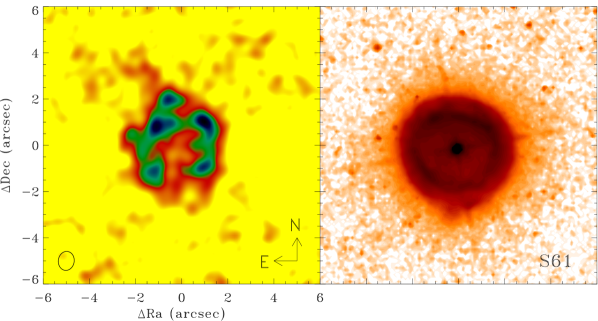
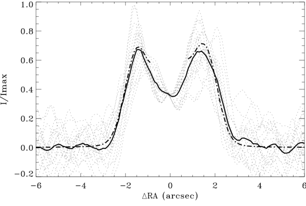
Figure 1: Upper-left panel: map of S61 at 17 GHz obtained with the ATCA. The ellipse in the lower-left corner visualises the synthesised beam. Upper-right panel: archival $\rm H\rm\alpha$ HST image. Lower panel: surface brightness profiles. Grey dotted lines: profiles extracted from 18 cuts across the radio nebula, passing through the centre, in steps of $10^{\circ}$. Black line: mean of the grey dotted lines. Black dash-dotted line: mean surface brightness of the $\rm H\rm\alpha$ image, derived from 18 cuts as explained before.

Table 1: Properties of the ATCA and ALMA maps.

Array	$\nu$	HPBW	LAS	PA	Peak	RMS
	$(\rm GHz)$	$(^{\prime\prime})$	$(^{\prime\prime})$	$(\rm deg)$	$(\rm mJy\,beam^{-1})$
ATCA	17	0.836$\times$0.686	6.5	-10.6	0.142	0.016
ATCA	23	0.628$\times$0.514	4.1	-10.8	0.121	0.032
ALMA	343	1.23$\times$0.95	6.7	-78.6	0.290	0.072

We performed ATCA observations of S61 (together with two other Magellanic LBVs) between January 20 and 23, 2012. We used the array in the most extended configuration (6 km) and the Compact Array Broadband Backend (CABB) “15 mm” receiver in continuum mode. We split the receiver bandwidth in two 2-GHz sub-bands, one centred at 17 GHz and the other at 23 GHz. This set-up was chosen in order to achieve enough spatial resolution to isolate possible contribution from the central source and also to obtain some spectral information. We observed the phase calibrator ICRF J052930.0$-$724528 for 1 minute, alternating with 7- or 10-min scans on target, depending on the weather. For the bandpass correction we performed observations on the calibrator QSO J1924$-$2914 each day as well as observations of the flux calibrator ICRF J193925.0$-$634245. We also performed reference pointing frequently (about every 1–2 h) to assure the pointing accuracy of the source observations. The total integration time obtained on each source was 8 hours.

We performed the data reduction and imaging using the MIRIAD package (Sault, Teuben, & Wright, 1995). We split the datasets in two parts (one per central frequency) and reduced them separately. For the data editing, flagging and calibration, we followed the standard calibration recipe for the millimetric band. We applied the opacity correction and flagged bad data, before calculating corrections for gains. We used observations of QSO J1924$-$2914, ICRF J193925.0$-$634245 and ICRF J052930.0$-$724528 for determining the bandpass, flux density and complex gain solutions, respectively. Once corrected, the visibilities were inverted by Fourier transform. We chose the natural weighting scheme of the visibilities, for best sensitivity. Deconvolution of the dirty images was performed using the Clark algorithm (Clark, 1980) and the selection of the clean components was done interactively. We then restored the clean components with the synthesised beam. Table 1 contains information about the synthesised beam (Half Power Beam Width, HPBW) and position angle (PA), largest angular scale (LAS), peak flux densities and rms-noise of the resulting images. At 17 GHz we detect above $3\sigma$ the nebular emission in its whole extension. At 23 GHz the map is noisy because of the system response to bad weather at higher frequencies. For this reason we do not show the 23 GHz data. The radio map at 17 GHz is illustrated in the upper-left panel of Fig. 1.

We also include in our analysis the 5.5 and 9-GHz data from the ATCA observations performed in 2011 by means of the CABB “4cm-Band” (4-10.8 GHz) receiver. These data were presented in Paper I.

2.2 The ALMA observation and data reduction

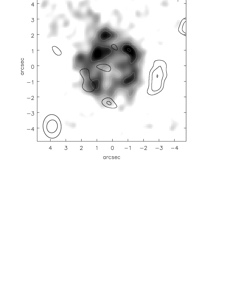
Figure 2: Raster ATCA 17 GHz map with $3,7\sigma$ contours overlaid (white). Black contours: from 2 to 4$\sigma$ levels in the ALMA map at 343 GHz. The big and small ellipses in the left bottom corner are respectively the ALMA and ATCA synthesised beams.

S61 was observed as part of an ALMA Cycle-2 project studying three Magellanic LBVs (2013.1.00450.S, PI Agliozzo). A single execution of 80 minutes total duration, including the three targets, was performed on 2014-12-26 with 40 12m antennas, with projected baselines from 10 to 245 m, and integration time per target of 16 minutes. A standard Band 7 continuum spectral setup was used, giving four 2-GHz width spectral windows of 128 channels of XX and YY polarisation correlations centred at approximately 336.5 (LSB), 338.5 (LSB), 348.5 (USB) and 350.5 (USB) GHz. Online, antenna focus was calibrated during an immediately preceding execution, and antenna pointing was calibrated on each calibrator source during the execution (all using Band 7). Scans at the science target tuning on bright quasar calibrators QSO J0538-4405 and Pictor A (PKS J0519-4546; an ALMA secondary flux calibrator ‘grid’ source) were used for interferometric bandpass and absolute flux scale calibration. Astronomical calibration of complex gain variation was made using scans on quasar calibrator QSO J0635-7516, interleaved with scans on the science targets approximately every six minutes. Of the 40 antennas in the array, 36 were fully used in the final reduction, with two more partially used due to issues in a subset of basebands and polarisations. Data were calibrated and imaged with the Common Astronomy Software Applications (CASA) package (McMullin et al., 2007).

Atmospheric conditions were marginal for the combination of frequency and necessarily high airmass (transit elevation $45^{\circ}$ for S61). Extra non-standard calibration steps were required to minimise image degradation due to phase smearing, to provide correct flux calibration, and to maximise sensitivity by allowing inclusion of shadowed antennas. As S61 was not detected, we defer discussion of these techniques to an article on the other sources in the sample (Agliozzo et al. 2016, submitted).

We derived the intensity image from naturally weighted visibilities to maximise sensitivity and image quality (minimise the impact of phase errors on the longer baselines). We imaged all spectral windows together ($343.5\,{\rm GHz}$ average; approximately $7.5\,{\rm GHz}$ usable bandwidth), yielding RMS noise of $72\,\mu{\rm Jy}\,{\rm beam^{-1}}$ in the image. This is compared to the proposed sensitivity of $40\,\mu{\rm Jy}\,{\rm beam^{-1}}$, which could not be achieved as no further executions were possible during the appropriate array configuration in Cycles 2 and 3. With this sensitivity, we did not detect the nebula. In Fig. 2 we show the 2, 3, and 4$\sigma$ contours in the ALMA map (in black) on top of the ATCA 17 GHz image. These contours do not have enough statistical significance. However, the elongated object West of the radio nebula has a peak at $4\sigma$, but it is difficult to associate it with S61. Details of the ALMA map are listed in Table 1. Deeper observations with ALMA may detect the nebular dust, and would certainly improve the constraints on the dust mass. This would be a good candidate for the potential “high sensitivity array” mode, combining all operational array elements ($12$ and $7\,{\rm m}$ antennas, typically at least 50 in total) in a single array with the 64-input Baseline correlator, when in the more compact 12m array configurations (this may be offered from Cycle 6 in 2018).

2.3 VLT/VISIR observations

Table 2: VISIR observational summary.

Date	Filter	Airmass	DIMM Seeing	PWV
			(arcsec)	(mm)
2015-09-03	PAH2$\_$2	1.576	1.35	3.2
2015-09-04	Q1	1.590	1.38	1.8

We proposed service-mode observations in the narrow bandwidth filters PAH2$\_$2 and Q1, centred respectively at 11.88 and 17.65 $\rm\mu$m. The observations were carried out between September 3rd and 4th, 2015. The observing mode was set for regular imaging, with pixel scale of 0.045 arcsec. The OBs were executed in conditions slightly worse (10%) than specified in the scheduling constraints. Table 2 contains a summary of the VISIR observations.

We have reduced the raw data by running the recipe $visir\_image\_combine.xml$ of the VISIR pipeline kit (version 4.0.7) in the environment Esoreflex 2.8. We have compared the calibrator (HD026967 and HD012524) flux densities and sensitivities with the ones provided by the observatory from the same nights, and have found consistent results. Due to the non-detection of the science target, the data reduction pipeline has performed a straight combining of the images while correcting for jitter information from the fits headers, rather than stacking individual images with the shift-and-add strategy. In the last step, the pipeline has converted the final (combined) images from ADU to $\rm Jy\,pixel^{-1}$ by adopting the conversion factor derived from the calibrators. The output of the pipeline is a single image of 851$\times$851 and 851$\times$508 pixels in the PAH2$\_$2 and Q1 filters, respectively. The two images are in unit of $\rm Jy\,pixel^{-1}$. The rms-noise in the images is 0.08 $\rm mJy\,pixel^{-1}$ and 2.1 $\rm mJy\,pixel^{-1}$, in the filters PAH2$\_$2 and Q1 respectively, which translate in noise of $\sim 40$ and $\sim 1000\,\rm mJy\,arcsec^{-2}$. We did not achieve the expected sensitivity (as estimated with the Exposure Time Calculator). This could be due to large scale emission. We estimate that to detect a point-like source with a signal-to-noise ratio of 3, it should be at least 15 $\rm mJy$ at 11.88 $\rm\mu$m and 430 $\rm mJy$ at 17.65 $\rm\mu$m.

2.4 Optical data

The $\rm H\rm\alpha$ Hubble Space Telescope (HST) data (Weis, 2003) where retrieved from the STScI data archive (proposal ID: 6540), as already described in Paper I. They were obtained with the Wide Field and Planetary Camera 2 (WFPC2) instrument using the $\rm H\rm\alpha$-equivalent filter F656N and reduced by the standard HST pipeline. We combined the dataset (four images with a 500 s exposure) following a standard procedure in IRAF to remove cosmic-ray artefacts and to improve the signal-to-noise ratio SNR. We also recalibrated the HST image astrometrically using the Naval Observatory Merged Astrometric Dataset (NOMAD) catalogue (Zacharias et al., 2005) for a corrected overlay with the radio images. Finally, we converted the HST/WFPC2 image from $\rm countspixel^{-1}\,\text{\AA}^{-1}$ units to $\rm erg\,cm^{-2}\,s^{-1}$ units, by multiplying with $2.9\times 10^{-16}\times 21.5$ (where 21.5 is the F656N filter bandwidth in Å).

3 The Radio Emission

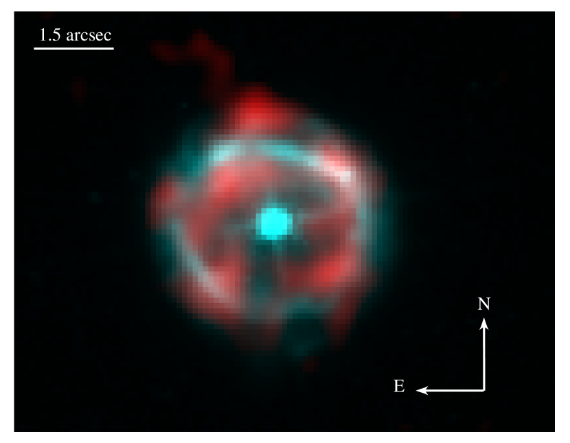
Figure 3: Two-colour image of S61. The red colour is the radio 17 GHz, the cyan one is the $\rm H\rm\alpha$.

Table 3: Observed flux densities, angular sizes and spectral index

S(5.5 GHz)	S(9 GHz)	S(17 GHz)	Size	$\langle\alpha\rangle$
(mJy)	(mJy)	(mJy)	(arcsec)
2.1$\pm$0.1	2.2$\pm$0.3	1.97$\pm$0.10	4.5$\times$4.9	-0.06$\pm$0.06

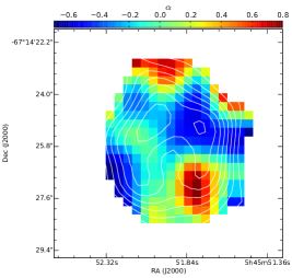
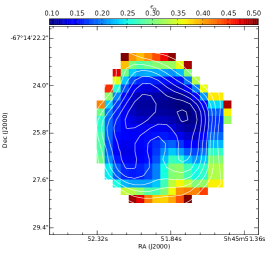
Figure 4: Left: spectral index map between 9 and 17 GHz. Right: spectral index error map. Before the computation, the map at 17 GHz was reconvolved to match the beam at 9 GHz. The white contours indicate flux densities above 3 $\sigma$ (at integer steps) of the 17 GHz emission at the 9 GHz resolution, and the cross represents the position of the star.

In the upper panel of Fig. 1, the radio map (left) is compared with the $\rm H\rm\alpha$ HST image (right). For a better visualisation of the nebular morphology, we also show in the lower panel the radial surface brightness profiles, extracted from 18 cuts (grey dotted lines) across the radio nebula, passing through the centre and successively rotated by $10^{\circ}$. The black line is the arithmetic mean of the grey dotted lines. In a similar way we derived the mean surface brightness of the $\rm H\rm\alpha$ HST image (black dash-dotted line), after convolving it with the radio beam. To block the emission of the central object in the $\rm H\rm\alpha$ image, we applied a mask at the position of the star. The image shows that there is more substructure in the radio than in the optical, as is clearly evident by comparing the surface profiles. At 17 GHz the nebula size is similar to the one in the $\rm H\rm\alpha$ image. A two-colour image of the 17 GHz and $\rm H\rm\alpha$ data is shown in Fig. 3. In the Northern part, apparently attached to the shell, there is a spur-emission, similar to G79.29+0.46 (e.g. Higgs, Wendker, & Landecker, 1994). This compact object does not have a counterpart either at lower frequencies or in the optical. It might indicate an optically thick medium at the radio wavelengths.

Weis (2003) reported that the optical nebula of S61 is expanding spherically and with a velocity of $\sim\!27\ \rm km\,s^{-1}$, although slightly red-shifted to the West and blue-shifted to the East, which they ascribed to a geometric distortion along the line of sight. The radio nebula at 17 GHz is consistent with the shell geometry and therefore we will take it into account to model the radio emission (Section 4).

Table 3 lists the spatially integrated flux density and its associated error at 17 GHz, together with the estimated nebula angular sizes (not deconvolved by the synthesised beam). The integrated flux density was determined by using the CASA viewer. In particular, we selected with the polygonal tool the area above $3\sigma$ level and integrated the emission over the nebula. The rms-noise in the map was evaluated in regions free of emission and hence flux density errors were estimated as $\epsilon=\sigma\sqrt{N}$, where $N$ is the number of independent beams in the selected region. Calibration flux density errors are usually negligible at these frequencies. The flux densities at 5.5 and 9 GHz derived in Paper I are also shown in the table.

From analysis of the spectral index, we can obtain information about the nature of the radio emission. We have computed the mean spectral index $\langle\alpha\rangle$ through a weighted fit of the power-law $S_{\nu}\propto\nu^{\alpha}$ between the flux densities at 5.5, 9 and 17 GHz in Table 3. The “global” spectral index $\langle\alpha\rangle=-0.06\pm 0.06$ is consistent with optically thin free-free emission. We have also obtained a spectral index map (per-pixel). To this end, the highest-resolution map (17 GHz) was re-gridded and convolved with the beam at lower frequency. We show the spectral index map between 17 GHz and 9 GHz (with the beam about $1.5\times 1.2$ arcsec², as in Paper I) and its associated error map in Fig. 4. Since calibration errors are negligible, in the maps the error in each pixel is mostly given by the sum in quadrature of the rms-noise in both the maps, in Jy pixel^-1 units. In the inner part of the nebula the mean spectral index is $\langle\alpha\rangle=-0.3\pm 0.2$ (where the error is the mean value in the error map), consistent with optically thin free-free emission. In the Southern (bottom) part we observe a higher spectral index ($\alpha_{max}=0.8\pm 0.3$) suggesting some mechanism of self-absorption of the free-free emission, due to, for instance, density clumps. The spectral index analysis may be biased by the fact that the interferometer is sensitive to different large and intermediate angular scales at different frequencies. However, the largest angular scales covered in the two datasets (12.9 and 6.5 arcsec at 9 and 17 GHz, respectively) are larger than the size of the nebula (Table 3). We also rely on a good uv coverage at the intermediate angular scales acquired during the observations.

4 Modelling the nebula

In Paper I we derived an estimate of the ionised mass in the S61 nebula from the 9 GHz ATCA map. Simply, the total ionised mass can be estimated if the density of particles and the volume of the nebula are known. For non-self-absorbed optically thin free-free emission, the electron density $n_{e}$ can be determined through the relation between the emission measure,

$$EM=\int_{0}^{s}{n_{e}^{2}\ \hbox{${\rm d}$}s\ [\rm pc\,cm^{-6}]},$$ (1)

and the optical depth $\tau_{ff}(\nu)$ at frequency $\nu$

$$\tau_{ff}(\nu)=8.24\times 10^{-2}\left(\frac{T_{e}}{\rm K}\right)^{-1.35}\left(\frac{\nu}{\rm 5\,GHz}\right)^{-2.1}\frac{EM}{\rm pc\,cm^{-6}}.$$ (2)

$\tau_{ff}(\nu)$ can be determined from the solution of the radiative transfer equation ($B_{\nu}=B_{bb}(T)\tau_{ff}(\nu)$) by setting as $B_{\nu}$ the radio brightness and by assuming a blackbody with temperature $T$ equal to the electron temperature $T_{e}$. Therefore, in Paper I we derived an average $n_{e}$ from the mean $EM$ (integrated over the nebula) and assumed as $s$ the transversal size of the nebula (measured on the radio map). With these values, we estimated for S61’s nebula an ionised mass of $\sim 0.8\,\rm M_{\odot}$. In reality, $n_{e}$ may vary inside the nebula. Furthermore, the geometrical depth $s$ may vary for different line of sights and then requires a proper geometrical model. Therefore, we propose a new approach to fit all the pixels of the radio maps with a global geometrical 3D density model of the nebula. Obviously, the nebula has to be spatially resolved. Instrumental effects on the nebula size due to bad resolution have to be negligible. If not, the estimated mass may be inaccurate.

4.1 3D density model Rhocube

We have written and make publicly available Rhocube (Nikutta & Agliozzo, 2016), a Python code to model 3D density distributions $\Varrho\!\!(x,y,z)$ on a discrete Cartesian grid, and their integrated 2D maps $\int\hbox{${\rm d}$}z\Varrho\!\!(x,y,z)$. It can be used for a range of applications; here we model with it the electron number density $n_{e}(x,y,z)$ in LBV shells, and from it compute the emission measure $EM$ given in Eq. (1).

The code repository includes several useful 3D density distributions, implemented as simple Python classes, e.g. a power-law shell, a truncated Gaussian shell, a constant-density torus, dual cones, and also classes for spiralling helical tubes. Other distributions can be easily added by the user. Convenient methods for shifts and rotations in 3D are also provided. If necessary, an arbitrary number of density distributions can be combined into the same model cube, and the integration $\int\hbox{${\rm d}$}z$ will be correctly performed through the joint density field. Please see Appendix A.4 and the code repository for usage examples of Rhocube, and for details of the implementation.

4.2 Bayesian parameter inference

We will apply Rhocube to our problem of estimating the physical parameters of the observed emission maps by modelling the underlying 3D electron density distribution $n_{e}(x,y,z)$. We employ a Bayesian approach and compute marginalized posterior density distributions of model parameters from the converged chains of Markov-Chain Monte Carlo (MCMC) runs. Bayes’ Theorem and the details of MCMC sampling are described in Appendix B. Our routines to fit Rhocube models to data are available as supplemental materials, in Section 7.

We begin with any 3D model for geometry of the nebula, e.g. a truncated Gaussian shell. At every sampling step of the MCMC procedure we draw a random vector $\theta$ of values for the free model parameters (e.g. the shell radius, width, lower and upper truncation radii, and $x$ and $y$ offsets). We then compute the 3D electron density distribution $n_{e}(x,y,z|\theta)$, and from it the squared integrated 2D map $EM_{\rm mod}=\int\!n_{e}^{2}(x,y)\,\hbox{${\rm d}$}z$. The normalisation of $n_{e}$ is at first arbitrary, but by comparison with the observed map $EM_{\rm obs}$ we can find a global scale $S$ such that the likelihood is maximised, or equivalently, the chi-squared statistic $\chi^{2}=\sum_{i}(d_{i}-S\cdot m_{i})^{2}/\sigma_{i}^{2}$ is minimised. The $d_{i}$ are the measured pixel values $EM_{\rm obs}^{\,i}$ (for unmasked pixels only), and $m_{i}$ their modelled counterparts. $S$ can be computed analytically (e.g. Nikutta, 2012). Note that the pixels $i$ are independent.

4.2.1 Application to the S61 nebula

Parameter	Units	9 GHz	17 GHz
Truncated Normal Shell
$r$	pc	$[0,0.3]$	$[0,0.3]$
$\sigma_{r}$	pc	$[0,0.7-r]$	$[0,0.6-r]$
$r_{\rm lo}$	pc	$[0,r]$	$[0,r]$
$r_{\rm up}$	pc	$[0,r+\sigma_{r}]$	$[0,r+\sigma_{r}]$
Power-Law Shell
$r_{in}$	pc	$[0,0.3]$	$[0,0.3]$
$r_{out}$	pc	$[r_{in},0.7]$	$[r_{out},0.6]$

Table 4: Uniform priors adopted for the truncated normal shell and the power-law shell models. The priors were chosen from visual inspection of the 9 GHz and 17 GHz maps and were limited to meaningful ranges.

Parameter	Units	Truncated Normal Shell
		MAP		Median
		9 GHz	17 GHz	9 GHz	17 GHz
		($\chi^{2}_{r}=46$)	($\chi^{2}_{r}=33$)
$r$	pc	0.19	0.30	$0.19^{+0.07}_{-0.09}$	$0.18^{+0.08}_{-0.09}$
$\sigma_{r}$	pc	0.50	0.30	$0.35^{+0.13}_{-0.15}$	$0.29^{+0.12}_{-0.13}$
$r_{\rm lo}$	pc	0.05	0.28	$0.08^{+0.09}_{-0.06}$	$0.07^{+0.09}_{-0.05}$
$r_{\rm up}$	pc	0.67	0.58	$0.35^{+0.15}_{-0.12}$	$0.31^{+0.13}_{-0.12}$
x-offset	pc	-0.07	-0.04	$0.00^{+0.09}_{-0.10}$	$0.00^{+0.03}_{-0.03}$
y-offset	pc	-0.08	-0.01	$0.00^{+0.09}_{-0.10}$	$-0.00^{+0.03}_{-0.03}$
Mion	$M_{\odot}$	0.29	0.13	$0.07^{+0.09}_{-0.04}$	$0.03^{+0.04}_{-0.02}$

Table 5: Inference of model parameters, as derived from data at 9 GHz and 17 GHz. A truncated normal spherical shell was used as a model. MAP = maximum-a-posteriori values. Median = median of marginalized posterior distributions, with $1\sigma$ confidence intervals. Note that M_ion is a derived quantity, i.e. not a free (modelled) parameter.

Parameter

Units

PLS exp=0 (constant-density shell)

PLS exp-1

PLS exp=-2

MAP

Median

MAP

Median

MAP

Median

9 GHz

17 GHz

9 GHz

17 GHz

9 GHz

17 GHz

9 GHz

17 GHz

9 GHz

17 GHz

9 GHz

17 GHz

($\chi^{2}_{r}=47$)

($\chi^{2}_{r}=22$)

($\chi^{2}_{r}=55$)

($\chi^{2}_{r}=48$)

($\chi^{2}_{r}=100$)

($\chi^{2}_{r}=74$)

$r_{in}$

pc

0.14

0.26

$0.16^{+0.09}_{-0.08}$

$0.17^{+0.08}_{-0.10}$

0.26

0.28

$0.16^{+0.09}_{-0.08}$

$0.17^{+0.08}_{-0.08}$

0.29

0.30

$0.16^{+0.09}_{-0.08}$

$0.16^{+0.09}_{-0.07}$

$r_{out}$

pc

0.69

0.59

$0.45^{+0.17}_{-0.18}$

$0.39^{+0.16}_{-0.15}$

0.69

0.57

$0.44^{+0.17}_{-0.18}$

$0.39^{+0.15}_{-0.12}$

0.69

0.59

$0.44^{+0.17}_{-0.18}$

$0.37^{+0.16}_{-0.15}$

x-offset

pc

-0.02

-0.02

$-0.00^{+0.02}_{-0.02}$

$0.00^{+0.01}_{-0.02}$

-0.03

-0.02

$0.00^{+0.02}_{-0.02}$

$-0.00^{+0.02}_{-0.02}$

-0.03

-0.02

$-0.00^{+0.02}_{-0.02}$

$0.00^{+0.01}_{-0.02}$

y-offset

pc

-0.03

0.00

$0.00^{+0.02}_{-0.02}$

$0.00^{+0.02}_{-0.02}$

-0.03

-0.02

$0.00^{+0.02}_{-0.02}$

$-0.00^{+0.02}_{-0.02}$

-0.03

-0.00

$-0.02^{+0.02}_{-0.02}$

$0.00^{+0.02}_{-0.01}$

Mion

$M_{\odot}$

0.31

0.14

$0.12^{+0.12}_{-0.09}$

$0.05^{+0.07}_{-0.04}$

0.30

0.12

$0.11^{+0.12}_{-0.08}$

$0.04^{+0.05}_{-0.03}$

0.27

0.11

$0.07^{+0.08}_{-0.05}$

$0.03^{+0.04}_{-0.02}$

Table 6: Inference of model parameters, in the case of power-law shells, with exponents: $0$ (i.e. constant-density shell), $-1$ and $-2$. MAP = maximum-a-posteriori values. Median = median of marginalized posterior distributions, with $1\sigma$ confidence intervals. Note that M_ion is a derived quantity, i.e. not a free (modelled) parameter.

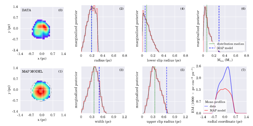
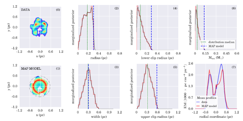
Figure 5: Results of fitting the 9 GHz (top two rows) and 17 GHz (bottom two rows) EM maps of S61 with truncated Gaussian shells. Panel (0) shows the data with linear sizes relative to the central pixel, with a $3\sigma$ mask applied. Panel (1) shows the model shell with parameters corresponding to the median values of all marginalized posterior distributions. Indicated as solid, dashed, and dotted circles are the median values of $r$, $r\pm\sigma_{r}$, and $r_{\rm up}$, respectively. Panels (2)-(6) show as red histogram the posteriors of four model parameters, and of the derived ionised mass M_ion. All histograms are normalized to unit area. The smooth black curve is a Gaussian kernel density estimation. The vertical blue-dashed and green-dotted lines indicate the maximum-a-posteriori (MAP) and median value of the MCMC chain, respectively. The blue dashed line in panel (6) locates the ionised mass value of the model shown in panel (1). Panel (7) illustrates azimuthal mean profiles derived from 18 extracted cuts along the EM (data: blue line; model: red line).

In the following we apply Rhocube together with MCMC and Bayesian inference to fit the EM maps obtained for S61 from the data at 9 GHz and 17 GHz. Note that the angular resolution in the map at 9 GHz is poor and affects the nebula size (Paper I). We only use this data to test our procedure and to compare the mean $EM_{\rm mod}$ and the derived ionised mass with those estimated in Paper I.

The radio maps of S61, while irregular, are indicative of a spherical matter distribution (e.g. Fig. 1, top-left). This is even more apparent in the H$\alpha$ map (Fig. 1, top-right; see also Pasquali, Nota, & Clampin, 1999; Weis, 2003). We therefore modelled with Rhocube the electron density distribution by using the following geometries: a truncated Gaussian (normal) shell and a power-law shell. For the truncated normal shell (hereafter TNS) the free parameters are six: the shell radius $r$, the width $\sigma_{r}$ of the Gaussian around $r$, the lower and upper clip radii $r_{\rm lo}$ and $r_{\rm up}$, and finally we allow for minute offsets in the plane of the sky, xoff and yoff, to account for possible de-centring of the observed shell. For the power-law shell (PLS) the free parameters are four: the inner and outer radii $r_{in}$ and $r_{out}$, xoff and yoff. For the PLS geometry we explored the cases with exponents: 0 (i.e. constant density shell), -1 and -2. We noticed that exponents smaller than -2 were producing lower-quality results and therefore we will not comment on them. We used uniform prior probability distributions (i.e. before introducing the model to the observed data) on the shell radius, width, and both clip radii for the TNS geometry, and for the inner and outer radii for the PLS geometry.

The ranges of these parameters must of course be limited to meaningful values. For convenience we converted the $x$ and $y$ pixel units in the maps from arcsec to parsec, assuming a distance of 48.5 kpc. Hence, from visual inspection of the map we adopted the values listed in Table 4. As priors of both offsets xoff and yoff we adopted very narrow Gaussians, truncated at $\pm 2$ pixels from the central pixel. The maps supplied to the code are $41\times 41$ and $101\times 101$ pixels (for the 9 GHz and 17 GHz data, respectively). In Tables 5 and 6 we show the resulting marginalized posteriors from the geometries mentioned before.

Figure 5 illustrates only the posteriors from the fit of the 9 GHz and 17 GHz data with a truncated Gaussian shell. These posteriors were obtained after drawing $2\times 10^{4}$ MCMC samples. Many fewer samples are necessary for convergence ($\sim$1000 may be sufficient), but more samples produce smoother histograms. In the figure we do not show the posteriors for the offsets xoff and yoff which are very narrow and centred, i.e. the shell is not significantly shifted from the central pixel. The MCMC chain histograms are shown in red, a Gaussian kernel density estimation is overplotted in black. Blue-dashed vertical lines indicate the single best-fit values (maximum-a-posteriori, MAP) of the MCMC chains, i.e. the combination of parameter values which simultaneously maximise the likelihood. Note that this need not be the “most typical” solution. Green-dotted lines mark the median values of the marginalized posterior PDFs. These statistics, and the $1\sigma$ confidence intervals around the median, are summarised in Table 5. Note that for the 9 GHz data PLS (with exp=0) equally produces a good-quality result. For the 17 GHz data the PLS (with exp=0) produces the best-fit. The MAP models (for unmasked pixels) have a formal $\chi^{2}_{r}$ as shown in the tables. While large values, considering the simple model and the clearly not entirely spherical/symmetric EM map, they are acceptable. In the figure we only show our favourite models, chosen because they produce more agreeable distributions and radial profiles. For this reason we now describe only them.

The distribution of shell radii (panels 2 in Fig. 5) is quite broad, but clearly peaks within the shell. The radial thickness of the Gaussian shell is symmetric around the peak in both panels 3. A similar comment can be given for the upper clip radius $r_{\rm up}$ (panels 5). The lower clip radius $r_{\rm lo}$ (panels 4) is left-bounded at 0, and the decline at the large-values tail is driven by our prior requirement. The observed 9 GHz and 17 GHz $EM_{obs}$ maps are shown in panels (0), and the model shell corresponding to the MAP model is shown in (1). This panel also shows with solid, dashed and dotted circles the median-model values of $r$, $r\pm\sigma_{r}$, and $r_{\rm up}$, respectively. Panel (7) illustrates azimuthal mean profiles derived from 18 extracted cuts along $EM_{obs}$ (blue line) and $EM_{\rm MAP}$ (red line). While the MAP model for the 9 GHz seems underestimated, the 17 GHz model profile is quite satisfactory.

As evident in the tables, different models (TNS, PLS exp=0, PLS exp=-1) produce similar-quality results, meaning that with the current data we cannot constrain the electron density distribution in the S61 nebula.

4.3 Ionised mass

Knowing the 3D distribution of the electron number density $n_{e}(x,y,z)$, we can now compute the total ionised mass contained in the shell via

$${\rm M_{ion}}=\frac{m_{p}}{M_{\odot}}\int\!\hbox{${\rm d}$}V\ n_{e}(x,y,z),$$ (3)

with $m_{p}$ and $M_{\odot}$ the proton and solar masses, under the assumption that the gas comprises only ionised hydrogen. For simple symmetric geometries and density distributions this integral can be evaluated analytically (e.g. a constant-density shell), but it might be significantly more challenging for more complicated geometries and more complex density fields. In our discretised 3D Cartesian grid, realizing that the volume of a 3D-voxel is $(\Delta x)^{3}$, because $\Delta x=\Delta y=\Delta z$, Eq. (3) simplifies to

$${\rm M_{ion}}=\frac{m_{p}}{M_{\odot}}\,(\Delta x)^{3}\sum_{i}n_{e}(x_{i},y_{i},z_{i}),$$ (4)

where the index $i$ runs over all voxels (recall they are independent).

Thanks to the MCMC approach we can use the entire converged chains of model parameter values to compute posterior distributions of derived quantities (i.e. not modelled quantities), such as the ionised mass here. The resulting marginalized posterior distribution for the TNS geometry is shown in panels (6) of Fig. 5, with the purpose to provide an example. In fact, as mentioned before, we do not have a statistically strong model to discern among the possible density distributions. However, it is comforting to see that all the models produce similar masses (see Tables 5 and 6).

The TNS model of the 9-GHz (17-GHz) data generates a peaked and skewed distribution of $M_{ion}$, with median $0.07^{+0.09}_{-0.04}\leavevmode\nobreak\ M_{\odot}$ ($0.03^{+0.04}_{-0.02}\leavevmode\nobreak\ M_{\odot}$). The MAP-model values are $0.29\leavevmode\nobreak\ M_{\odot}$ and $0.13\leavevmode\nobreak\ M_{\odot}$. These are located always in the right side of the distribution, probably due to our prior requirements to fit the shell within the edge of the nebula, rather than the edge of the image frame. We remind the reader that the modelling of the 9 GHz data was proposed in order to test the code and to compare the results with our previous estimation ($\sim$0.8 $M_{\odot}$, Agliozzo et al., 2012). The value derived with this new approach is about 2.7 times smaller than the previous estimate. However, because of the asymmetry of the nebula at 9 GHz, the model seems to underestimate, on average, $EM_{obs}$ (see Panel 7 in Fig. 5). According to this, the two methods may not disagree each other.The advantage of the proposed new method is that it requires no assumptions about the nebula depth $s$.

The derived mass from the fits of the 17 GHz data ($0.11-0.14\,\rm M_{\odot}$) are more representative, because of the smaller $\chi^{2}_{r}$ than the 9 GHz data. The mean profile of $EM_{MAP}$ reproduces satisfactorily $EM_{obs}$ (see bottom Panel 7 in Fig. 5). More importantly, the angular resolution achieved at 9 GHz affects the nebular size, resulting in a larger volume to model. For further analysis we will then adopt the MAP model from the fit of the 17 GHz data.

The mass estimated here are at least an order of magnitude smaller than the one derived by Pasquali, Nota, & Clampin (1999) from the $\rm H\rm\alpha$ luminosity and from optical emission lines. The discrepancy may be due to a combination of different assumptions and methods. For instance, Pasquali, Nota, & Clampin (1999) assumed for the LMC a distance of 51.2 kpc and measured a size for the nebula of 7.3 arcsec (i.e., 1.8 pc) from an image with a poorer resolution. Their estimation of the average electron density was also uncertain due to uncertainties of the [SII] 6717/6731 ratio. It would be interesting to compare our results with integral field unit observations of the nebula around S61.

As shown in Section 3, there are hints of inhomogeneities in the nebula. Following Abbott, Bieging, & Churchwell (1981), who described the radio spectrum of a clumped stellar wind, we can assume discrete gas clumps of relatively higher density ($n_{H}$), embedded in a lower-density medium ($n_{L}$). Both the clumps and the inter-clump medium are assumed optically thin. The clumps are distributed randomly throughout the volume of the nebula. If we define $f$ as the fractional volume which contains material at density $n_{H}$, then Eq. (1) becomes

$$EM=\int_{0}^{s}{(fn_{H}^{2}+(1-f)n_{L}^{2})\ \hbox{${\rm d}$}s\ }.$$ (5)

The ionised mass in the nebula can be underestimated if not corrected for clumpiness. In fact, in the simple case of an empty inter-clump medium ($n_{L}=0$), it is possible to demonstrate that $M\propto S_{\nu}^{\frac{1}{2}}f^{-\frac{1}{2}}$. For a filling factor $f=0.5$ the ionised mass would be about 41$\%$ larger than in the case of a homogeneous nebula. For a more generic case, the factor to correct the estimated ionised mass is $(fn_{H}^{2}+(1-f)n_{L}^{2})^{\frac{1}{2}}$. The ionised mass could also be underestimated in the emitting regions with a positive spectral index. In the specific case of S61, where $\alpha\sim 0.8$, the optical depth is $\lesssim 1$. Moreover, the region with positive $\alpha$ is small. We can assume that the underestimation of mass is negligible.

By using our model, we can derive the ionising photon flux as

$${\rm F_{UV}}=(\Delta x)^{3}\,\beta_{2}\sum_{i}n_{e}^{2}(x_{i},y_{i},z_{i}),$$ (6)

with $\beta_{2}$ the recombination coefficient of the second energy level of H. It is still not known if the nebula is density or ionisation bounded, therefore we have to keep in mind that this could be a lower limit. We find $\rm Log(F_{UV})=44.5$, which corresponds to a supergiant of spectral type later than B3. This is too cold compared with S61’s star (Crowther & Smith, 1997; Pasquali, Nota, & Clampin, 1999). Note that the recombination time for such a nebula would be typically of some thousands years, implying that LBV variability from the ionising source would be negligible. This may indicate that the nebula is density-bounded and that part of the stellar UV flux escapes from the nebula.

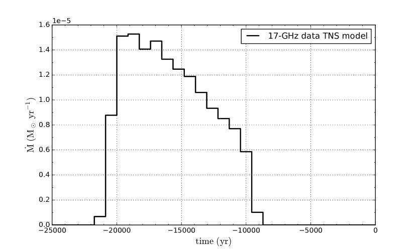
Figure 6: Mass-loss rate of S61 as derived from fitting the circumstellar nebula. Each bin of the histogram corresponds to $\sim 850\,\rm yr$. The plot does not contain information about the present-day mass-loss rate.

5 Discussion

5.1 The mass-loss history

Starting from our best model in Section 4, we now derive the mass-loss history of S61 with high temporal resolution, keeping in mind that we could not constrain the electron density distribution.

If we know the expansion velocity of this nebula, each voxel of our datacube corresponds to a kinematical age. For instance, in the case of S61 the expansion velocity is 27 $\rm km\,s^{-1}$ (Weis, 2003) and each voxel in the model of the 17 GHz data has a 1-D size equal to 0.1 arcsec, which, at the assumed distance of the LMC (48.5 kpc) corresponds to 7.3$\times 10^{11}\,\rm km$ and therefore to a kinematical interval of $\sim 850\,\rm yr$. We know the mass in each voxel and therefore we can derive the average mass-loss rate $dM/dt$ in intervals of $850\,\rm yr$. According to the shell geometry adopted for the S61 nebula, we can assume that the star has lost mass isotropically. We can finally integrate $dM/dt$ over shells of radius $r$ and thickness $dr$, where $r$ can vary between 0 and $\frac{N}{2}+1$ ($N$ is the number of pixels in each dimension of the cube). The resulting mass-loss rates for S61 are shown in Fig. 6. In this particular example, the peak of the mass-loss has occurred at epoch $\sim 19100$ yr with a rate of $1.5\times 10^{-5}\,\rm M_{\odot}\,yr^{-1}$. However, we note that the finite resolution due to the synthesised beam may mean that the real distribution is less smooth.

The mass-loss rates derived in Fig. 6 are consistent with our non-detection of the stellar wind in the radio maps. If we assume a spherical mass-loss for the star and then the model in Panagia & Felli (1975), with a terminal velocity of 250 $\rm km\,s^{-1}$ (Crowther & Smith, 1997), an electron temperature of 6120 K (Pasquali, Nota, & Clampin, 1999) and a flux density equal to 3 times the noise in the map at 17 GHz, we derive a 3$\sigma$ upper limit of $\sim 2.3\times 10^{-5}$ $\rm M_{\odot}\,yr^{-1}$, for a fully ionised wind with solar abundances. This upper limit is consistent with the mass-loss rate of $\sim 1.1\times 10^{-5}$ $\rm M_{\odot}\,yr^{-1}$ derived by Crowther & Smith (1997), which would be within the distribution in Fig. 6. The value by Pasquali et al. (1997) of $\sim 2.2\times 10^{-5}$ $\rm M_{\odot}\,yr^{-1}$ derived from H emission lines seems inconsistent with the radio non-detection.

We now compare the mass-loss history with the empirical mass-loss rate, as predicted for O, B normal supergiants following the procedure described in Vink, de Koter, & Lamers (2000). We first assume the stellar parameters by Crowther & Smith (1997) ($T_{eff}=27.6\,\rm kK$, $\log\left(\frac{L}{L_{\odot}}\right)=5.76$ and $v_{\infty}=250\,\rm km\,s^{-1}$), a metallicity of $Z=0.5\,\rm Z_{\odot}$ and an initial stellar mass of $\sim 60\,\rm M_{\odot}$ (according to the evolutionary tracks by Schaller et al., 1992). The small nebular mass derived in the previous section suggests that the star has a stellar mass similar to its initial value and then the mass-loss rate is comparable to the one relative to the O, B main sequence stars (the reduced stellar mass of LBVs causes a strong increase in the mass-loss rate with respect to normal O, B supergiants, as showed by Vink & de Koter, 2002). The empirical mass-loss rate derived with the mentioned parameters is $6.6\times 10^{-6}\,\rm M_{\sun}\,yr^{-1}$, which is close to the average value of the distribution in Fig. 6. The consequence of this result is either that the mass-loss occurred with a constant wind (constant density model) or the mass-loss rates varied due to excursion through the bi-stability jump (power-law electron density model). In this latter case the bi-stability jump for S61 would occur at $T_{eff}\sim 23.5\,\rm kK$, with a mass-loss rate of $3.3\times 10^{-5}\,\rm M_{\odot}\,yr^{-1}$, which is consistent with the peak in Fig. 6 within a factor of $\sim 2$. In both cases we can probably exclude that S61 lost mass through eruptions, as normal stellar winds perfectly explain the observations. If we instead use the stellar parameters by Pasquali et al. (1997) ($T_{eff}=36.1\,\rm kK$, $\log\left(\frac{L}{L_{\odot}}\right)=6.1$), the derived empirical mass-loss rate is $7.0\times 10^{-5}\,\rm M_{\sun}\,yr^{-1}$, which is far higher than our observational values derived in the previous section.

5.2 Extinction map and nebular dust

We have derived the extinction map of S61 by comparing pixel-by-pixel the highest-resolution radio image (17 GHz) with the HST $\rm H\rm\alpha$ image, as the two emissions trace the same gas (Paper I). According to Pottasch (1984), if the optical $\rm H\rm\alpha$ emission is due to the de-excitation of the recombined H atom and the radio continuum emission to free-free encounters, one can determine the extinction of the optical line by comparing the two brightnesses, as

$$F_{\nu(expected)}=2.51\times 10^{7}T_{e}^{0.53}\nu^{-0.1}YF_{\rm H_{\beta}}\hskip 14.22636pt\rm[Jy]$$ (7)

where $T_{e}$ is the electron temperature of the nebula in units of K, $\nu$ is the radio frequency in GHz, Y is a factor incorporating the ionised He/H ratios (assumed to be 1, as in Paper I) and

$$F_{\rm H_{\beta}}=\frac{1}{2.859}\left(\frac{T_{e}}{10^{4}}\right)^{0.07}\,F_{\rm H_{\alpha}}$$ (8)

for the theoretical Balmer decrement.

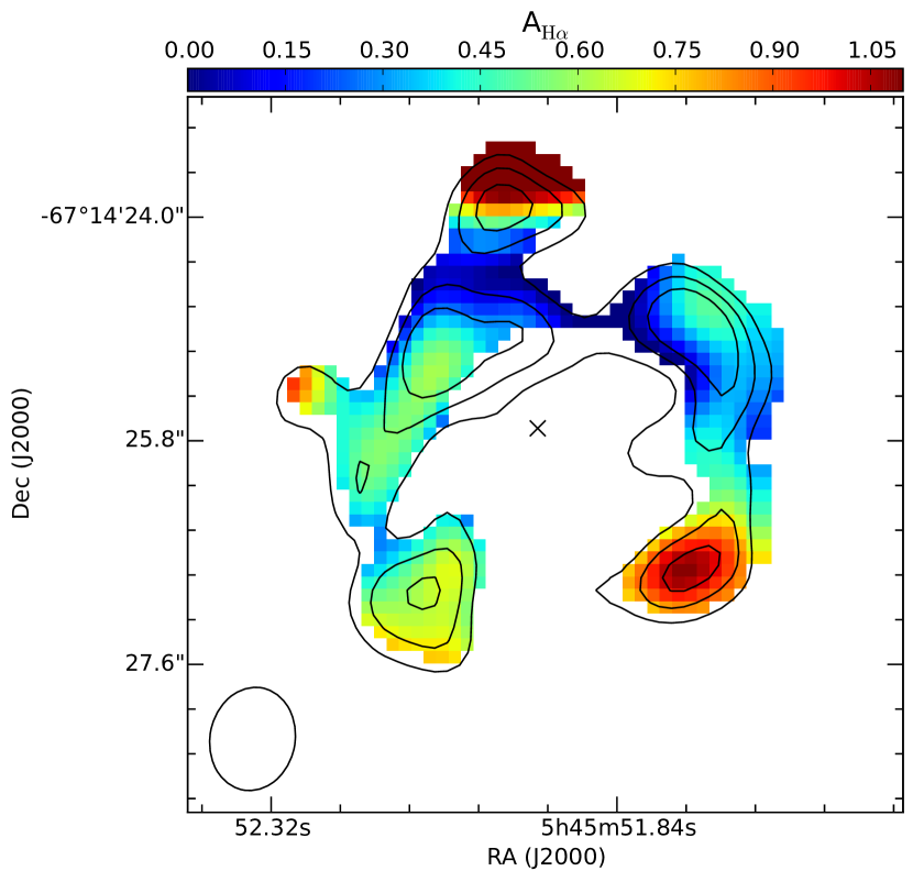
Figure 7: Extinction map in $\rm H\rm\alpha$, as derived by comparing the $\rm H\rm\alpha$ recombination line and the centimetre (17 GHz) emission above $5\sigma$. The central star was masked with a circular aperture in the optical image. The black contours are 5, 7 and 9$\sigma$ levels of the radio emission and the black ellipse is the resolution. The black cross represents the position of the star, according to the Simbad Database.

We re-gridded the HST image to the same grid of the radio map and converted it to Jy pixel^-1 unit. We convolved the optical image with the radio beam (elliptical Gaussian with HPBW as in Table 1). Adopting as electron temperature $6120\,\rm K$ (Pasquali, Nota, & Clampin, 1999), we derive the expected radio map from the $\rm H\rm\alpha$ recombination-line emission. Keeping in mind that we want to estimate the expected free-free emission from the optical line in the nebula, we masked the $\rm H\rm\alpha$ emission from the star. Finally, the extinction map in $\rm H\rm\alpha$ was derived as $2.5\,\log(F_{\rm 17\,GHz\,(obs)}/F_{\rm 17\,GHz\,(expected)})$ in every common pixel with brightness above 5$\sigma$, where $\sigma$ was computed by summing in quadrature the noise in the maps and calibration uncertainties (however negligible). As a result of this procedure, we obtained the extinction map illustrated in Fig. 7.

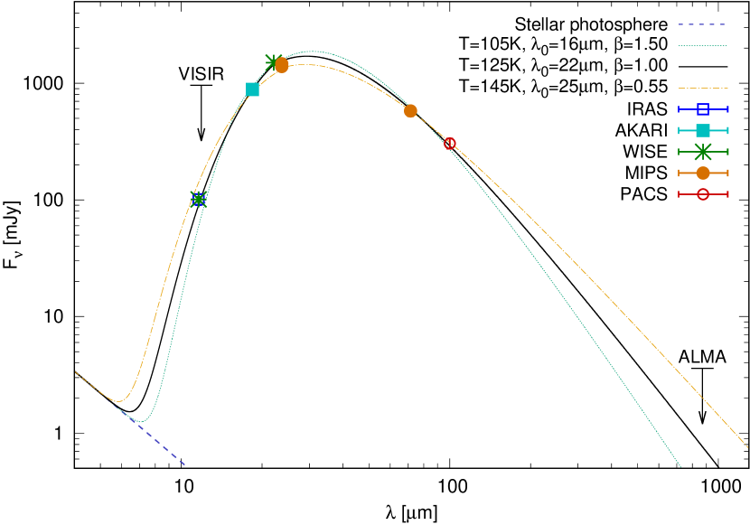
Figure 8: Flux density distribution of S61 derived by using the flux densities in the IR catalogues. The continuum lines represent the fit grey-body functions obtained for three values of the parameter $\beta$. The 3$\sigma$ upper limit spatially integrated flux densities at the VISIR and ALMA observing wavelengths (11.88 $\rm\mu m$ and 875 $\rm\mu m$, respectively) are also shown.

Small extinction due to dust is evident across the whole region. The range of values for A_Hα across the nebula is between $\sim$0.1 and 1.09. The maximum value for A_Hα is 1.8 and corresponds to the spur-object in the Northern (upper) part.

To derive a range of possible characteristic temperatures for the dust that extinguishes the optical emission, we fitted the flux density distribution from the mid- to the far-IR. We consulted the IR catalogues with the VizieR tool (Ochsenbein, Bauer, & Marcout, 2000) at the position of S61, and we extracted the flux densities in the WISE bands W3 and W4 (Cutri et al., 2012a; Cutri & et al., 2012b), AKARI L18W at 18 $\rm\mu m$ (Ishihara et al., 2010a, b), Spitzer MIPS at 24 and 70 $\rm\mu m$ (Ardila et al., 2010a, b) and Herschel PACS at 100 $\rm\mu m$ (Meixner et al., 2013). We fitted a single-temperature greybody with power-law opacity index $\beta$ at longer wavelengths and constant opacity at shorter wavelengths (e.g. Backman & Paresce, 1993),

$$F_{\nu}(\lambda)\propto\tau(\lambda)B_{\nu}(\lambda),\quad\tau(\lambda)=\left\{\begin{matrix}\tau_{0}&\lambda\leq\lambda_{0}\\ \tau_{0}\left({\lambda\over\lambda_{0}}\right)^{-\beta}&\lambda>\lambda_{0}\end{matrix}\right.$$ (9)

We found a range of characteristic temperatures between $\sim\!105$ to $145\,\rm K$ by varying the parameter $\beta$ (we explored the cases for $\beta=0.55,1$ and $1.5$) and $\lambda_{0}$ (between 18 and 25 $\rm\mu m$). The modified black-body that best fits the data is the one represented with a dark continuum line in the figure, with $\beta=1.0$. Note that $\beta=1.0$ implies either the existence of relatively large grains or different dust components (of different temperatures). The latter is usually observed in Galactic LBVNe and the temperature of the dust decreases with increasing distance from the star (e.g. Hutsemekers, 1997; Buemi et al., submitted to MNRAS, ).

According to the flux density distributions in Fig. 8, the expected flux densities $F_{\nu}$ at the VISIR PAH2$\_$2 and Q1 central wavelengths ($11.88$ and $17.65\,\rm\mu m$) are: $105\pm 40\,\rm mJy$ and $764\pm 50\,\rm mJy$, respectively. If this emission arises from a point-like source close to the star as observed in other candidate LBVs (e.g. G79.29+0.46, Agliozzo et al., 2014), we would have detected it with VISIR. We deduce then that the dust is spread out over the nebula, at angular scales that our observations were not sensitive to. Similarly, we have derived the expected ALMA flux density at 343 GHz: $0.8^{+1.2}_{-0.5}\,\rm mJy$. Even for the most favourable case for the dust ($\beta\sim 0.5$, corresponding to optically thick large grains), the sensitivity achieved with only one execution was not sufficient to detect the thermal emission at sub-mm wavelengths. In fact, with an expected flux density of $2\,\rm mJy$ (case $\beta=0.55$), spread across 16.7 ALMA synthesised beams, the average brightness would be $0.12\,\rm mJy\,beam^{-1}$ and a sensitivity of $40\,\rm\mu Jy\,beam^{-1}$ was needed for a $3\sigma$ detection. Note that the extrapolated flux density at the ALMA frequency is consistent with the upper limit derived from the map: the rms-noise ($72\,\rm\mu Jy$), integrated over the area corresponding the ionised nebula, yields a 3$\sigma$ upper limit of $\sim 3.6\,\rm mJy$. Using the flux density extracted from the best fit (case $\beta=1.0$) at the ALMA frequency 343 GHz (see Fig. 8), we derived a dust mass $M_{d}=5\times 10^{-3}$ to $2.7\times 10^{-2}\,\rm M_{\odot}$, considering that $M_{d}=S_{\nu}\,D^{2}/(B_{\nu}(T)\,\kappa_{\nu})$, and assuming $\kappa_{343\rm\,GHz}=1\rm\,cm^{2}\,g^{-1}$. This means a low gas-to-dust ratio for the LMC. It suggests that the sub-mm emission might be even lower than that computed from the flux density distributions based on the mid- and far-IR data.

The extinction map resembles the dusty nebula around the Galactic LBV IRAS 18576$+$034 (Buemi et al., 2010). This was also observed with VISIR in the filters PAH2$\_$2 and Q1. They derived for the mid-IR nebula a dust component of temperature ranging from 130 to 160 K. IRAS 18576$+$034 has a mid-IR nebula of 7 arcsec diameter, corresponding to 0.35 pc at the distance of 10 kpc. It has a physical size which is about half that of S61, but in the sky the two sources have similar angular size. We rescaled the IRAS 18576$+$034 VISIR maps to the distance of the LMC, and we derived from the maps a mean value of $0.3\,\rm mJy\,pixel^{-1}$ in the PAH2$\_$2 filter and $1.3\,\rm mJy\,pixel^{-1}$ in the Q1 filter. This means that with our VISIR observations, we would have detected at $\sim 3.5\sigma$ in the PAH2$\_$2 filter image a nebula like IRAS 18576$+$034. The sensitivity reached in band Q1 would have not been sufficient to detect the nebula. Buemi et al. (2010) derived for IRAS 18576$+$034 a dust mass of $\sim 4.5-6.5\times 10^{-3}\,\rm M_{\odot}$ (depending on the assumed dust composition) and Umana et al. (2005) derived a mass of $\sim 2\,\rm M_{\odot}$ for the ionised gas. This suggests the dust content in the nebula around S61 is similar in mass to that estimated in IRAS 18576$+$034. Conversely, the ionised mass in S61 is only a small fraction (1/20th) of the mass in the IRAS 18576$+$034 nebula, despite S61’s nebula diameter ($\sim 1.2\rm\,pc$) being about 3.5 times bigger than IRAS 18576$+$034 ($\sim 0.35\rm\,pc$). We recall, however, that IRAS 18576$+$034 has an estimated bolometric luminosity higher than S61 ($\log\left(\frac{L}{L_{\odot}}\right)=6.4$, Ueta et al., 2001) and the mass, through the mass-loss’ quadratic dependence on luminosity, has a stronger effect than the metallicity. The inner shell around Wray 15-751, which has a luminosity similar to S61, extends up to $1\rm\,pc$, similar to S61 and has gas and dust masses of $1.7\pm 0.6\,\rm M_{\odot}$ and $\sim 3.5\times 10^{-2}\,\rm M_{\odot}$, respectively (Vamvatira-Nakou et al., 2013), more massive than the S61 nebula. This may suggest that S61’s mass-loss has been less efficient over time than the mentioned Galactic LBVs. The dust production does not seem significantly different. However, a potential issue for this comparison is the larger uncertainty of the Galactic LBVs distances than those of the Magellanic objects.

6 Conclusions

In this work we presented high spatial resolution observations from the radio to the mid-IR of the nebula associated with the candidate LBV S61. It was detected only in the centimetre band. The nebula has a morphology resembling a shell, as in the optical, but in the radio there is more sub-structure. The emission mechanism is optically thin free-free, as evidenced by the spectral index map, although there are regions that suggest self-absorption.

We developed and made publicly available a code in Python that permits to model the 3-D electron density distribution and to derive the mass in the nebula. We tried different geometries for the shell (truncated Gaussian, constant density and power-law $n_{e}\propto r^{-1}$ and $\propto r^{-2}$) and we found that at least three of these geometries give similar-quality results. For all the well-fitting models, the derived ionised mass is always about 0.1 M_⊙, which is an order of magnitude smaller than previous estimates and also a few factors smaller than the mass of similar Galactic objects. The nebula is very likely density bounded, meaning that part of the stellar UV flux escapes from the nebula. As an application of our modelled electron density distribution, we also show how to derive the mass-loss history with high-temporal resolution ($\sim$ 850 yr). The derived mass-loss rates are consistent with the empirical mass-loss rate for S61, implying that the nebula was likely formed by stellar winds, rather than eruptive phenomena. The present-day mass-loss is $\lesssim 2\times 10^{-5}$ $\rm M_{\odot}\,yr^{-1}$.

Based on the extinction map derived from the radio map and the $\rm H_{\alpha}$ HST image, we have explored the possibility that the nebular regions with higher spectral index are dusty, by means of high-resolution mid-IR and sub-mm observations. We did not detect any point-like source, or compact regions associated with the clumps, neither with VISIR nor with ALMA. The fit of the IR flux distribution from space telescope observations suggest the presence of dust with a range of characteristic temperatures of $125\pm 20\,\rm K$ and dust mass $M_{d}$ of $10^{-3}$ to $10^{-2}\,\rm M_{\odot}$. Based on the observations with VISIR and ALMA, we exclude that the IR emission arises from a point-like source. The dust producing the infrared emission observed by space telescopes must be searched for within the angular scales of the ionised gas ($\sim$1–5 arcsec). The dust is distributed in an optically thin configuration over the radio nebula, but not uniformly, as shown in the extinction map. The VISIR observations did not reach the required sensitivity to detect such extended thermal emission. With the ALMA observations, we obtained better sensitivity to study thermal emission, but still the nebula was not detected. We estimate that the thermal emission could be detected by deeper ALMA observations in the future, including 7m antennas to enhance sensitivity on larger angular scales.

7 Supplements

Rhocube (Nikutta & Agliozzo, 2016) is a general-use, stand-alone code and is distributed as such in the following git repository: https://github.com/rnikutta/rhocube . In the spirit of scientific reproducibility we also share with the reader all scripts and supplementary codes that we have used in this work, specifically the MCMC sampling and Bayesian inference functions that make use of Rhocube, the functions to compute the ionised mass within a density model and the mass-loss history, and some plotting routines. A git repository for this manuscript, holding all supplementary files including the data FITS files, is accessible at: https://github.com/rnikutta/s61-supplements

Appendix A Brief introduction to RHOCUBE

A.1 Principles

Rhocube computes a 3D density field $\Varrho\!\!(x,y,z)$ on a Cartesian, right-handed grid, with $x$ pointing to the right, $y$ pointing up, and $z$ pointing to the viewer. The grid resolution is set by the user upon model instantiation. Several models with density distributions of common interest are provided, and new ones can be easily added by the user. At the time of writing, the (mnemonically named) provided models are: PowerLawShell, TruncatedNormalShell, ConstantDensityTorus, ConstantDensityDualCone, Helix3D. The latter takes as the envelope parameter the imaginary surface on which the helical tube spirals (dual cone or cylinder). The models are implemented as Python classes, and all inherit basic functionality, such as e.g. 3D rotations and $x,y$ offsets, from a common class Cube.

Every model has a number of free parameters, e.g. for PowerLawShell the inner and outer radii rin and rout, and the radial power-law index pow. Two lateral offsets xoff and yoff to de-center the density distribution in the image plane are available to all the models, as are the rotation angles tiltx, tilty, tiltz, which, when provided, rotate the entire 3D density field about the respective axes. They are of course ineffectual for spherically symmetric density distributions. Figure 9 shows a few examples of integrated maps that can be computed with the code.

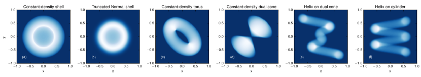
Figure 9: Example gallery of some $z$-integrated model density maps that can be generated with Rhocube. $x$ and $y$ are in relative linear units. The colour map is scaled to the image maxima. (a) Constant-density shell with four free parameters: inner and outer shell radii, and the centre offsets xoff and yoff. (b) A truncated Gaussian-density shell with 6 free parameters: radius, width of the Gaussian, left and right cut-off radii, two offsets. (c) A constant-density torus with six free parameters: radius, cross-section, two tilt angles, two offsets. (d) A dual-cone with six free parameters: height, opening angle, two tilts, two offsets. (e) Helical tube on the surface of a dual cone, with the free parameters radius at top of the cone, number of turns taken from origin, tube diameter, three tilts, two offsets. (f) Like (e) but on the surface of a cylinder. An arbitrary combination of models, with relative total masses as free parameters, is also possible.

A.2 Usage

The workflow with Rhocube is straight-forward:

• Instantiate a model (e.g. PowerLawShell)

• Call the instance with a set of parameter values

• Retrieve/access the 3D density cube and/or 2D $z$-integrated image

Instantiating a model generates the Cartesian grid (with requested resolution), and provides it with general methods to manipulate the density distribution (e.g. 3D rotations and shifts in $(x,y,z)$). Once the model is created, it can be called any number of times with a set of numerical arguments which are the values that the free model parameters should assume. Each call computes the corresponding 3D density field and also integrates that field along the $z$ axis, storing the resulting 2D image as a member of the model instance. If the smoothing parameter was set to a float value, then $\Varrho\!\!(x,y,z)$ will be smoothed with a 3D Gaussian kernel (see Sec. A.3.2). Listing 1 show a simple example instantiating and calling a simple model.

Listing 1: Instantiating and calling a model.

⬇

from models import PowerLawShell as PLS

mod = PLS(101,exponent=0.,smoothing=1.) # 0. for const.dens. shell

args = (0.1,0.7,0,0,None) # rin,rout,xoff,yoff,weight

mod(*args)

The resulting $\Varrho\!\!(x,y,z)$ is now in mod.rho (as 3D array), and the summation along $z$ direction is in mod.image. If you wanted to vary the parameters of this model:

⬇

args = (0.3,0.5,0,0.3,None) # rin,rout,xoff,yoff,weight

mod(*args)

If a transform function is provided during instantiation, it will be applied to $\Varrho\!\!(x,y,z)$ before integration (see Sec. A.3.1). If during calling the weight parameter is set to a float value, the sum $\sum_{i}\Varrho\!\!(x,y,z)$ (of the possibly transformed $\Varrho\!\!(x,y,z)$) over all voxels will be normalized to that value. Listing 2 shows an example.

Listing 2: Using transform function and weight parameter.

⬇

from rhocube import PowerTransform

mod = PLS(101,exponent=-1.,smoothing=1.,transform=PowerTransform(2.))

args = (0.1,0.7,0,0,1.) # rin,rout,xoff,yoff,weight

mod(*args)

print model.rho.sum()

1.0 # the specified ’weight’

A.3 Special methods

A.3.1 The ’transform’ function

An optional transform function $f(\Varrho)$ can be passed as an argument when creating a model instance. The transforms are implemented as simple Python classes. A transform will be applied to the density field before $z$-integration, i.e. $\int\!\hbox{${\rm d}$}z\,f(\Varrho\!\!(x,y,z))$ will be computed. In our case for instance, squaring of the electron number density before integration is required by Eq. (1). If the supplied $f(\Varrho)$ class also provides an inverse function, e.g. $f^{-1}=\sqrt{\cdot}$ when $f=(\cdot)^{2}$, then the entire 3D cube $\Varrho\!\!(x,y,z)$ with correct scaling can also be computed and accessed by the user. Some common transform classes are provided with Rhocube, e.g. PowerTransform, which we use for the squaring mentioned above (with argument pow=2), or LogTransform which computes a base-base logarithm of $\Varrho\!\!(x,y,z)$. Another provided transform is GenericTransform which can take any parameter-free Numpy function and inverse (the defaults are func=’sin’ and inversefunc=’arcsin’). Custom transform functions can be easily added.

A.3.2 Smoothing of the 3D density field

Upon instantiating a model, the smoothing parameter can be specified. If smoothing is a float value, it is the width (in standard deviations) of a 3D Gaussian kernel that $\Varrho\!\!(x,y,z)$ will be convolved with, resulting in a smoothed 3D density distribution. Smoothing does preserve the total $\sum_{i}\Varrho\!\!(x,y,z)$, where $i$ runs over all voxels. smoothing=1.0 is the default, and does not alter the resulting structure significantly. If smoothing=None, no smoothing will be applied.

A.4 Providing own density distributions

The Cube class provides two convenience objects and methods to compute the 3D density $\Varrho\!\!(x,y,z)$, which can (but don’t need to) be utilised by the actual model upon instantiation. The two methods are computeR and buildkdtree.

A.4.1 X,Y,Z coordinate arrays

By default, 3D Cartesian coordinate grids X,Y,and Z are computed upon instantiation of the Cube class, and each holds the $x$ or $y$ or $z$ coordinates of the voxel centers, in fractional units of a cube with extent [-1,1] along every axis. They can be used to compute arbitrary dependencies $\Varrho\!\!(x,y,z)$.

A.4.2 Distance array

If computeR=True is passed to Cube during model instantiation, then the class will also compute a 3D radius grid R(x,y,z), i.e. a cube of $\rm npix^{3}$ voxels, each holding its own radial distance from the cube center. This $R$ cube can then be used inside the model to compute a distance-dependent density as $\Varrho\!(R)$. This method is used in all azimuthally-symmetric models that come with Rhocube, e.g. PowerLawShell and TruncatedNormalShell.

Below we show in a simple example how one can construct a custom 3D density model that computes a spherically symmetric $\Varrho\!(R)$ which varies as the cosine of distance, i.e. $\Varrho\!(R)\propto\cos(R)$.

⬇

class CosineShell(Cube):

def __init__(self,npix):

Cube.__init__(self,npix,computeR=True)

def __call__(self):

self.get_rho()

def get_rho(self):

self.rho = N.cos(self.R)

self.apply_rho_ops() # shift, rotate3d, smoothing

You can then use it simply like this:

⬇

import CosineShell

mod = CosineShell(101) # 101 pixels along each cube axis

mod() # this model has no free parameters

Please see the built-in model classes for more details and ideas.

A.4.3 k-d tree

Rhocube also supports non-symmetric or irregular density distributions. One example might me the (also provided) model for a helix that winds along some prescribed parametric curve. For fast computation of all voxels within some orthogonal distance from the parametric curve (i.e. within a ’tube’), we utilise the second helper method in Cube, namely a k-d tree (Bentley, 1975). The Helix3D model works like this:

⬇

from models import Helix3D

mod = Helix3D(101,envelope=’dualcone’) # ’cylinder’ also available

args = (0.8,1,0.2,0,0,90,0,0,None) # h,nturns,tilt_x/y/z,

# xoff,yoff,weight

mod(*args)

Note that the initial building of the k-d tree is a $\mathcal{O}(n\log^{2}{}n)$ operation. The subsequent lookups are then much faster. Please see the Helix3D class for more details of the implementation.

Appendix B Bayesian parameter inference

B.1 Conditional probability and Bayes’ Theorem

Estimating the most likely physical parameters (inputs) of a model whose output is compared to observed data, is by far the most common scenario of Bayesian statistics. In our case, the inputs are the geometrical parameters of the modelled 3D electron density distribution $n_{e}(x,y,z)$, and the outputs are the modelled emission measure (EM) maps. They are compared to the observed EM maps of a given LBV shell.

We must vary the free model parameters, with the objective of minimizing the deviation of the resulting model EM map and the data EM map (for instance $\chi^{2}$ if the data errors can be assumed Gaussian). We desire not only to estimate the best-fit parameters, but to quantify their uncertainty, or the confidence that we can have in the results. The most natural approach to this common parameter estimation problem is Bayesian inference. Using notation borrowed from statistical literature, Bayes’ Theorem

$$Posterior\equiv p(\vec{\theta}|\vec{D})=\frac{p(\vec{\theta})\,p(\vec{D}|\vec{\theta})}{p(\vec{D})}\equiv\frac{Prior\times Likelihood}{Evidence}$$ (10)

provides a straight-forward prescription how to compute the joint posterior probability distribution (PDF) $p(\vec{\theta}|\vec{D})$ of a possibly multi-variate vector of model parameters $\vec{\theta}=(\theta_{1},\theta_{2},\ldots)$, given the observed data vector $\vec{D}$. The posterior PDF distribution is simply a product of a prior PDF $p(\vec{\theta})$ (i.e. any knowledge we may have of the model parameter distribution before introducing the data) with the likelihood that the given parameter values generate a model that is compatible with the data. For normally distributed errors the likelihood is $p(\vec{D}|\vec{\theta})\propto\exp(-\chi^{2}/2)$ (see e.g. Trotta, 2008).

The evidence $p(\vec{D})$ in Eq. (10) is the normalisation (integral of the multi-dimensional posterior PDF), ensuring that the total probability be unity. For the sole purpose of parameter inference, it is not necessary to compute the evidence explicitly, since it does not change the shape of the posterior PDF. It is instead sufficient to re-normalize the posterior to unit volume a posteriori. Thus, for parameter inference, only the relation $p(\vec{\theta}|\vec{D})\propto p(\vec{\theta})\,p(\vec{D}|\vec{\theta})$ is relevant. Of particular interest for the interpretation of results are the marginalized 1D posterior distributions, each integrated over all model parameters but the one in question

$$p(\theta_{i}|\vec{D})=\int\!\hbox{${\rm d}$}\theta_{1}\hbox{${\rm d}$}\theta_{1}\ldots\hbox{${\rm d}$}\theta_{i-1}\hbox{${\rm d}$}\theta_{i+1}\ldots\hbox{${\rm d}$}\theta_{N}\ p(\vec{D}|\vec{\theta}).$$ (11)

Every $\theta_{i}\in\vec{\theta}$ is one of the free model parameters, and every $\theta_{j}\neq\theta_{i}$ is a so-called nuisance parameter when computing the marginalized posterior PDF of $\theta_{i}$. Hence the common expression “marginalize over the nuisance parameters”. In our application, the marginalized posteriors are shown in panels (2)–(5) in Fig. 5. Panel (6) shows the posterior PDF of a derived quantity, which in the Bayesian approach is trivial to compute, and in the “classical” approach, impossible.

B.2 MCMC sampling

The $N$ model parameters span an $N$-dimensional volume which grows exponentially with the number of parameters. It very quickly becomes impractical to sample the entire volume. Fortunately, for many problems only small sub-volumes are relevant, i.e. the likelihood is only high in small regions of the parameter volume. Several methods to sample preferentially these highly significant regions have been proposed. The best-known is probably Markov-Chain Monte Carlo sampling (MCMC). A particularly straight-forward MCMC formalism is the Metropolis-Hastings algorithm introduced by Metropolis et al. (1953) and later generalized by Hastings (1970). It can be shown that the proposal joint PDF from which the algorithm samples eventually converges towards the sought-after target posterior PDF. MCMC thus generates a chain of samples (for every model parameter $\theta_{i}$), whose histogram is the marginalized posterior $p(\theta_{i}|\vec{D})$.

A common way to characterise the marginal PDFs is to compute the median (0.5 percentile of the cumulative distribution function, CDF), and as the confidence interval (or “credible interval”) the boundaries of an inter-percentile range. For Gaussian PDFs this can be the $\pm 1\sigma$ interval around the median, i.e. the range [0.158–0.841] of the CDF. For (slightly) asymmetric PDFs, an inter-quartile range is often used, i.e. [0.25–0.75]. While the posteriors in our application are not always Gaussian, for consistency we will report as the confidence interval the $\pm 1\sigma$ range around the median throughout.

References

- Abbott, Bieging, & Churchwell (1981) Abbott D. C., Bieging J. H., Churchwell E., 1981, ApJ, 250, 645
- Agliozzo et al. (2012) Agliozzo C., Umana G., Trigilio C., Buemi C., Leto P., Ingallinera A., Franzen T., Noriega-Crespo A., 2012, MNRAS, 426, 181
- Agliozzo et al. (2014) Agliozzo C., Noriega-Crespo A., Umana G., Flagey N., Buemi C., Ingallinera A., Trigilio C., Leto P., 2014, MNRAS, 440, 1391
- Ardila et al. (2010a) Ardila D. R., et al., 2010a, ApJS, 191, 301
- Ardila et al. (2010b) Ardila D. R., et al., 2010b, yCat, 219,
- Backman & Paresce (1993) Backman, D. E. and Paresce, F., 1993, Protostars and Planets III, 1253
- Bentley (1975) Bentley, J. L., 1975, Commun. ACM, 18, 9
- Bohannan & Walborn (1989) Bohannan B., Walborn N. R., 1989, PASP, 101, 520
- Buemi et al. (2010) Buemi C. S., Umana G., Trigilio C., Leto P., Hora J. L., 2010, ApJ, 721, 1404
- (10) Buemi C. S., Trigilio C., Leto P., Umana G., Ingallinera A., Cavallaro F., Cerrigone L., Agliozzo C., Bufano F., Riggi S., Molinari S., Schilliro F., 2016, submitted to MNRAS
- Clark (1980) Clark B. G., 1980, A&A, 89, 377
- Clark, Larionov,& Arkharov (2005) Clark J. S., Larionov V. M., Arkharov A., 2005, A&A, 435, 239
- Conti & Frost (1976) Conti P. S., Frost S. A., 1976, BAAS, 8, 340
- Crowther & Smith (1997) Crowther P. A., Smith L. J., 1997, A&A, 320, 500
- Cutri et al. (2012a) Cutri R. M., et al., 2012a, wise.rept,
- Cutri & et al. (2012b) Cutri R. M., et al., 2012b, yCat, 2311,
- Davidson & Humphreys (2012) Davidson K., Humphreys R. M., 2012, ASSL, 384,
- Duncan & White (2002) Duncan R. A., White S. M., 2002, MNRAS, 330, 63
- Fullerton, Massa, & Prinja (2006) Fullerton A. W., Massa D. L., Prinja R. K., 2006, ApJ, 637, 1025
- Gvaramadze, Kniazev, & Fabrika (2010) Gvaramadze V. V., Kniazev A. Y., Fabrika S., 2010, MNRAS, 405, 1047
- Hastings (1970) Hastings, W. K., 1970, Biometrika, 57, 97-109
- Higgs, Wendker, & Landecker (1994) Higgs L. A., Wendker H. J., Landecker T. L., 1994, A&A, 291, 295
- Humphreys & Davidson (1994) Humphreys R. M., Davidson K., 1994, PASP, 106, 1025
- Humphreys et al. (2016) Humphreys R. M., Weis K., Davidson K., Gordon M. S., 2016, ApJ, 825, 64
- Hutsemekers (1997) Hutsemekers D., 1997, ASPC, 120, 316
- Ishihara et al. (2010a) Ishihara D., et al., 2010a, A&A, 514, A1
- Ishihara et al. (2010b) Ishihara D., et al., 2010b, yCat, 2297,
- Jiménez-Esteban, Rizzo, & Palau (2010) Jiménez-Esteban F. M., Rizzo J. R., Palau A., 2010, ApJ, 713, 429
- Kraemer et al. (2010) Kraemer K. E., et al., 2010, AJ, 139, 2319
- Lamers, Snow, & Lindholm (1995) Lamers H. J. G. L. M., Snow T. P., Lindholm D. M., 1995, ApJ, 455, 269
- Lang et al. (2005) Lang C. C., Johnson K. E., Goss W. M., Rodríguez L. F., 2005, AJ, 130, 2185
- McMullin et al. (2007) McMullin J. P., Waters B., Schiebel D., Young W., Golap K., 2007, ASPC, 376, 127
- Meixner et al. (2013) Meixner M., et al., 2013, AJ, 146, 62
- Metropolis et al. (1953) Metropolis N., et al., 1953, The Journal of Chemical Physics, 21, 6
- Nazé, Rauw, & Hutsemékers (2012) Nazé Y., Rauw G., Hutsemékers D., 2012, A&A, 538, A47
- Nikutta (2012) Nikutta R., 2012, PhD thesis, University of Kentucky, http://uknowledge.uky.edu/physastron_etds/8/
- Nikutta & Agliozzo (2016) Nikutta R., Agliozzo C., 2016, rnikutta/rhocube: 1.0.1, https://doi.org/10.5281/zenodo.160465
- Ochsenbein, Bauer, & Marcout (2000) Ochsenbein F., Bauer P., Marcout J., 2000, A&AS, 143, 23
- Oskinova, Hamann, & Feldmeier (2007) Oskinova L. M., Hamann W.-R., Feldmeier A., 2007, A&A, 476, 1331
- Panagia & Felli (1975) Panagia N., Felli M., 1975, A&A, 39, 1
- Paron et al. (2012) Paron S., Combi J. A., Petriella A., Giacani E., 2012, A&A, 543, A23
- Pasquali et al. (1997) Pasquali A., Langer N., Schmutz W., Leitherer C., Nota A., Hubeny I., Moffat A. F. J., 1997, ApJ, 478, 340
- Pasquali, Nota, & Clampin (1999) Pasquali A., Nota A., Clampin M., 1999, A&A, 343, 536
- Pauldrach & Puls (1990) Pauldrach A. W. A., Puls J., 1990, A&A, 237, 409
- Petriella, Paron, & Giacani (2012) Petriella A., Paron S. A., Giacani E. B., 2012, A&A, 538, A14
- Pottasch (1984) Pottasch, S. R. 1984, Planetary Nebulae: A Study of Late Stages of Stellar Evolution, (Dordrecht: D. Reidel)
- Sault, Teuben, & Wright (1995) Sault R. J., Teuben P. J., Wright M. C. H., 1995, ASPC, 77, 433
- Schaller et al. (1992) Schaller G., Schaerer D., Meynet G., Maeder A., 1992, A&AS, 96, 269
- Smith et al. (1998) Smith L. J., Nota A., Pasquali A., Leitherer C., Clampin M., Crowther P. A., 1998, ApJ, 503, 278
- Smith & Owocki (2006) Smith N., Owocki S. P., 2006, ApJ, 645, L45
- Stahl (1986) Stahl O., 1986, A&A, 164, 321
- Trotta (2008) Trotta R., 2008, ConPh, 49, 71
- Ueta et al. (2001) Ueta T., Meixner M., Dayal A., Deutsch L. K., Fazio G. G., Hora J. L., Hoffmann W. F., 2001, ApJ, 548, 1020
- Umana et al. (2005) Umana G., Buemi C. S., Trigilio C., Leto P., 2005, A&A, 437, L1
- Umana et al. (2010) Umana G., Buemi C. S., Trigilio C., Leto P., Hora J. L., 2010, ApJ, 718, 1036
- Umana et al. (2011a) Umana G., Buemi C. S., Trigilio C., Leto P., Hora J. L., Fazio G., 2011, BSRSL, 80, 335
- Umana et al. (2011b) Umana G., Buemi C. S., Trigilio C., Leto P., Agliozzo C., Ingallinera A., Noriega-Crespo A., Hora J. L., 2011b, ApJ, 739, L11
- Umana et al. (2012) Umana G., et al., 2012, MNRAS, 427, 2975
- Vamvatira-Nakou et al. (2013) Vamvatira-Nakou C., Hutsemékers D., Royer P., Nazé Y., Magain P., Exter K., Waelkens C., Groenewegen M. A. T., 2013, A&A, 557, A20
- Vamvatira-Nakou et al. (2015) Vamvatira-Nakou C., Hutsemékers D., Royer P., Cox N. L. J., Nazé Y., Rauw G., Waelkens C., Groenewegen M. A. T., 2015, A&A, 578, A108
- van Genderen (2001) van Genderen A. M., 2001, A&A, 366, 508
- Vink, de Koter, & Lamers (1999) Vink J. S., de Koter A., Lamers H. J. G. L. M., 1999, A&A, 350, 181
- Vink, de Koter, & Lamers (2000) Vink J. S., de Koter A., Lamers H. J. G. L. M., 2000, A&A, 362, 295
- Vink & de Koter (2002) Vink J. S., de Koter A., 2002, A&A, 393, 543
- Vink & Gräfener (2012) Vink J. S., Gräfener G., 2012, ApJ, 751, L34
- Wachter et al. (2011) Wachter S., Mauerhan J., van Dyk S., Hoard D. W., Morris P., 2011, BSRSL, 80, 291
- Walborn (1977) Walborn N. R., 1977, ApJ, 215, 53
- Walborn (1982) Walborn N. R., 1982, ApJ, 256, 452
- Weis (2003) Weis K., 2003, A&A, 408, 205
- Weis (2008) Weis K., 2008, cihw.conf, 183
- Zacharias et al. (2005) Zacharias N., McCallon H. L., Kopan E., Cutri R. M., 2005, HiA, 13, 603