Mating quadratic maps with the modular group II

Abstract

In 1994 S. Bullett and C. Penrose introduced the one complex parameter family of $(2:2)$ holomorphic correspondences $\mathcal{F}_{a}$:

$$\left(\frac{aw-1}{w-1}\right)^{2}+\left(\frac{aw-1}{w-1}\right)\left(\frac{az+1}{z+1}\right)+\left(\frac{az+1}{z+1}\right)^{2}=3$$

and proved that for every value of $a\in[4,7]\subset\mathbb{R}$ the correspondence $\mathcal{F}_{a}$ is a mating between a quadratic polynomial $Q_{c}(z)=z^{2}+c,\,\,c\in\mathbb{R}$, and the modular group $\Gamma=PSL(2,\mathbb{Z})$. They conjectured that this is the case for every member of the family $\mathcal{F}_{a}$ which has $a$ in the connectedness locus.

We show here that matings between the modular group and rational maps in the parabolic quadratic family $Per_{1}(1)$ provide a better model: we prove that every member of the family $\mathcal{F}_{a}$ which has $a$ in the connectedness locus is such a mating.

1 Introduction

The analogies between the iteration of holomorphic maps and the action of Kleinian groups were first enumerated by Sullivan in the mid 1980s. His landmark paper [S], where he proved the conjecture of Fatou that there are no wandering domains for a rational map on the Riemann sphere, includes the first version of what it is now called Sullivan’s dictionary, in which definitions, theorems and conjectures in the world of holomorphic maps are related to analogous definitions, theorems and conjectures in the world of Kleinian groups. Sullivan draws attention to deep parallels between the Fatou set $F_{f}$ and Julia set $J_{f}$ of a holomorphic map $f$ on $\widehat{\mathbb{C}}$, and the ordinary set $\Omega(G)$ and limit set $\Lambda(G)$ respectively of a finitely generated Kleinian group $G$ acting on $\widehat{\mathbb{C}}$, and his proof of the no wandering domains theorem for rational maps is inspired by the method used to prove Ahlfors’ finiteness theorem in the world of Kleinian groups.

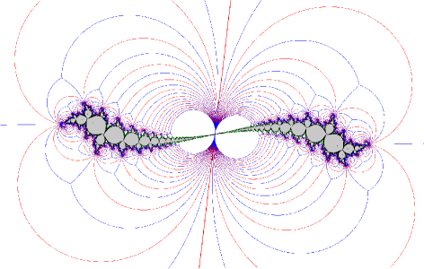
Figure 1: Limit set for $\mathcal{F}_{a}$, $a=4.565+0.420i$.

Both rational maps and finitely generated Kleinian groups can be regarded as particular cases of correspondences. An $n$-to-$m$ holomorphic correspondence on $\widehat{\mathbb{C}}$ is a multi-valued map $\mathcal{F}:z\rightarrow w$ defined by a polynomial relation $P(z,w)=0$. A rational map $f(z)=p(z)/q(z)$ becomes an $n$-to-$1$ correspondence defined by $P(z,w)=0$, where $P(z,w)=wq(z)-p(z)$, and any finitely generated Kleinian group $G$ with generators

$$\gamma_{j}(z)=\frac{a_{j}z+b_{j}}{c_{j}z+d_{j}}$$

can be regarded as an $(n:n)$ correspondence by taking

$$P(z,w)=\prod_{j=1}^{n}\left(w(c_{j}z+d_{j})-(a_{j}z+b_{j})\right).$$

For example, since

$$\alpha(z)=z+1\quad{\rm and}\quad\beta(z)=\frac{z}{z+1}$$

generate the modular group $\Gamma=PSL(2,\mathbb{Z})$, the orbits of $\Gamma$ on $\widehat{\mathbb{C}}$ are the orbits of the $(2:2)$ correspondence defined by

$$(w-(z+1))(w(z+1)-z)=0.$$

The study of iterated holomorphic correspondences was initiated by Fatou [F] in 1922, with an analysis of a family of examples ‘sur lesquels’, he remarks, ‘on voit apparaitre déjà certaines propriétés, assez différentes de celles auxquelles donnent lieu les cas d’itération déjà étudiés’ [‘in which one already sees the appearence of certain properties somewhat different from those arising in the cases of iteration studied up till now’]. He concludes his article with the comment that one may treat various examples of iterated algebraic functions in an analogous fashion, ‘mais une théorie générale de ce problème ne parait pas facile. Nous pensons pouvoir y revenir ultérieurement’ [‘but a general theory for this problem does not seem easy. We hope to return to this in the future’]. The next developments of which we are aware came in the 1990s, when McMullen and Sullivan in their foundational work [MS], defined a (one-dimensional) holomorphic dynamical system to be a collection of holomorphic relations on a complex $1$-manifold, and developed a common framework in which rational maps, Kleinian groups and holomorphic correspondences can be treated simultaneously. At around the same time researchers in integrable systems [BV] were investigating the complexity of symmetric holomorphic correspondences associated with elliptic curves, a topic also prefigured in the introduction to Fatou’s article.

Also in the 1990s, the first author and C. Penrose observed behaviour such as that illustrated in Figure 1, in a particular family of $(2:2)$ correspondences, namely the one parameter family $\mathcal{F}_{a}$ defined by

$$\left(\frac{aw-1}{w-1}\right)^{2}+\left(\frac{aw-1}{w-1}\right)\left(\frac{az+1}{z+1}\right)+\left(\frac{az+1}{z+1}\right)^{2}=3.$$

Computer plots appeared to show two copies (denoted in this article by $\Lambda_{a,-}$ and $\Lambda_{a,+}$) of the filled Julia set of a quadratic polynomial, together with an action of the modular group on the complement (denoted $\Omega_{a}$ here), prompting the question as to whether in the world of holomorphic correspondences there might exist ‘matings’ between quadratic polynomials and the modular group. Bullett and Penrose [BP] constructed an abstract combinatorial mating between the modular group and any member of the quadratic family which has connected and locally connected filled Julia set (see Section 1.1). Holomorphic correspondences realising these combinatorial matings are holomorphic realisations of Minkowski’s question mark function [Min], a homeomorphism from the unit interval to the positive real line which sends a real number expressed in binary to a real number with a corresponding continued fraction expression. On the binary expression side of the mating is the Douady-Hubbard coding of rays for quadratic polynomials, which is key to combinatorial descriptions of Julia sets and renormalisation theory. On the continued fraction side, the action of the modular group is related to the generation of Farey sequences of rationals, and thence to the Riemann Hypothesis (we thank Charles Tresser for drawing our attention to the work of Franel [Fr] and Landau [Lan], showing that the Riemann Hypothesis is equivalent to certain conditions concerning the uniformity of distribution of such sequences).

The main result of [BP] is that for $a$ in the real interval $[4,7]$ the holomorphic correspondence $\mathcal{F}_{a}$ is indeed a mating between a (real) quadratic polynomial and the modular group. More generally, Bullett and Penrose conjectured that each $\mathcal{F}_{a}$ for which the parameter $a$ is in the connectedness locus for the family is a mating between a quadratic polynomial and the modular group. Their conjecture was subsequently proved for a large class of values of the parameter $a$, by applying Haissinsky’s technique of ‘pinching’ to polynomial-like maps (see [BHai]). But the technique is not applicable for all values of $a$ in the connectedness locus, and we would argue that the root cause of the difficulty is that the family of quadratic polynomials is the wrong model for the problem. Whatever the value of $a$, the branch of $\mathcal{F}_{a}$ which fixes $z=0$ is parabolic, with multiplier at the parabolic fixed point equal to 1 (see Proposition 3.6). This fact makes the use of polynomial-like mappings tricky and finally inefficient, and suggests that the optimum description of the correspondences $\mathcal{F}_{a}$ might be as matings between the modular group and members of some family of parabolic quadratic maps. As we shall demonstrate below, this is indeed the case, the family of maps being

$$P_{A}:z\to z+\frac{1}{z}+A,\quad A\in\mathbb{C},$$

which we recall are the quadratic rational maps with a parabolic fixed point of multiplier $1$ at infinity and critical points at $\pm 1$. Note that $P_{A^{\prime}}$ is conformally conjugate to $P_{A^{\prime\prime}}$ if and only if $A^{\prime}=\pm A^{\prime\prime}$; in Milnor’s notation the set of (conformal) conjugacy classes is denoted $Per_{1}(1)$.

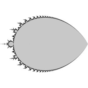
Figure 2: The modular Mandelbrot set $M_{\Gamma}$

Definition 1.1.

We say that ${\mathcal{F}}_{a}$ is a mating between the rational quadratic map $P_{A}:z\to z+1/z+A$ and the modular group $\Gamma=PSL(2,{\mathbb{Z}})$ if

(i) the $2$-to-$1$ branch of ${\mathcal{F}}_{a}$ for which $\Lambda_{a,-}$ is invariant is hybrid equivalent to $P_{A}$ on $\Lambda_{a,-}$, and

(ii) when restricted to a $(2:2)$ correspondence from $\Omega_{a}$ to itself, ${\mathcal{F}}_{a}$ is conformally conjugate to the pair of Möbius transformations $\{\alpha,\ \beta\}$ from the complex upper half plane ${\mathbb{H}}$ to itself.

Formal definitions of the sets $\Lambda_{a,-}$, $\Lambda_{a,+}$, and $\Omega_{a}$ are given in Section 3. In the same Section we also define the Klein combination locus $\mathcal{K}\subset\mathbb{C}$ and the connectedness locus ${\mathcal{C}}_{\Gamma}\subset{\mathcal{K}}$ of the family of correspondences ${\mathcal{F}}_{a}$. Given these concepts, we are in a position to state the main result of this paper:

Main Theorem.

For every $a\in{\mathcal{C}}_{\Gamma}$ the correspondence ${\mathcal{F}}_{a}$ is a mating between some rational map $P_{A}:z\to z+1/z+A$ and $\Gamma$.

The layout of this paper is as follows. In Section 2 we assemble facts concerning Fatou coordinates and parabolic-like mappings that will be needed later. In Section 3 we investigate some dynamical properties of the family $\mathcal{F}_{a}$ and in Section 4 we prove:

Theorem A.

For every $a\in{\mathcal{C}}_{\Gamma}$, when restricted to a $(2:2)$ correspondence from $\Omega_{a}$ to itself, ${\mathcal{F}}_{a}$ is conformally conjugate to the pair of Möbius transformations $\{\alpha:z\to z+1,\ \beta:z\to z/(z+1)\}$ from the complex upper half plane ${\mathbb{H}}$ to itself.

In Section 5 we prove that every ${\mathcal{F}}_{a}$ with $a$ in the Klein combination locus $\mathcal{K}$ can be surgically modified to become a single-valued parabolic-like map in the sense of [L] on a neighbourhood of the backward limit set $\Lambda_{a,-}$. Since this parabolic-like map can then be straightened ([L]) into a rational map of the form $P_{A}:z\to z+1/z+A$, we obtain the following:

Theorem B.

For every parameter value $a\in{\mathcal{K}}$, after a surgery supported outside the limit set, the branch of $\mathcal{F}_{a}$ fixing $\Lambda_{a,-}$ restricts to a parabolic-like mapping, and therefore on $\Lambda_{a,-}$ is hybrid equivalent to a member of the family $Per_{1}(1)$ of quadratic rational maps.

Note that since the Julia set of a rational map is the closure of the set of repelling periodic points, and quasiconformal maps preserve the nature of periodic points, the theorem implies the following:

Corollary 1.2.

For each $a\in{\mathcal{K}}$, the boundary of $\Lambda_{a,-}$ is the closure of the set of repelling periodic points of the branch of $\mathcal{F}_{a}$ fixing $\Lambda_{a,-}$.

The Main Theorem is a consequence of Theorems A and B.

As we shall see, the closed disc ${\mathcal{D}}=\{a:|a-4|\leq 3\}$ is contained in the Klein combination locus ${\mathcal{K}}$ (apart from the point $a=1$, where $\mathcal{F}_{a}$ is undefined). Let $M_{\Gamma}$ denote the modular Mandelbrot set ${\mathcal{C}}_{\Gamma}\cap{\mathcal{D}}$. This set $M_{\Gamma}$ (Figure 2), which we believe to be the whole of ${\mathcal{C}}_{\Gamma}$, and which visibly resembles the classical Mandelbrot set, was first plotted in [BP]. In [BL1] we investigate the dynamics of the family $\mathcal{F}_{a}$, and in particular we prove a new inequality of Yoccoz type which has as consequences the facts that $M_{\Gamma}$ is contained in a lune within ${\mathcal{D}}$ of internal angle strictly less than $\pi$, and that for all $a\in M_{\Gamma}$ the limit set $\Lambda_{a,-}$ is contained in a dynamical space lune of internal angle strictly less than $\pi$. This in turn will allow us in [BL2] to undertake the surgery of Theorem B in a sufficiently uniform manner to deduce that $M_{\Gamma}$ is homeomorphic to the connectedness locus $M_{1}$ of the family $Per_{1}(1)$. Together with the proof announced by Pascale Roesch and Carsten Petersen that $M_{1}$ is homeomorphic to the classical Mandelbrot set $M$, this will finally prove that $M_{\Gamma}$ is homeomorphic to $M$.

Acknowledgements. The authors are very grateful to Adam Epstein for first suggesting to them in 2011 that parabolic-like mappings might be applied to the family of correspondences $\mathcal{F}_{a}$, and to Adam Epstein, Carsten Petersen and Pascale Roesch for very helpful discussions at various stages of the work reported on here. This research has been partially supported by EU Marie-Curie IRSES Brazilian-European partnership in Dynamical Systems (FP7-PEOPLE-2012-IRSES 318999 BREUDS) and the Fundação de amparo a pesquisa do estado de São Paulo (Fapesp, process 2013/20480-7).

2 Preliminaries

This section is devoted to a summary of results we will use during the article.

2.1 Petals and Fatou coordinates

A holomorphic map $g(z)=z+bz^{2}+\ldots$, with $b\neq 0$, defined in a neighbourhood of the origin, has a parabolic fixed point at the origin with multiplicity 1. A complex number v points in the repelling direction if $b$v is real and positive, and a complex number w points in the attracting direction if $b$w is real and negative. An open set in a neigbourhood of the origin is called an attracting petal if it is mapped into itself and if each orbit eventually absorbed by it converges to the origin from the attracting direction v. Similarly, a repelling petal is an open set contained in its image and with orbits escaping from the origin in the repelling direction w.

There exists a well-established body of knowledge concerning attracting and repelling petals at parabolic fixed points of holomorphic functions $g$, and Fatou coordinates on these petals. We shall make use of petals with the properties listed in the following Proposition.

Proposition 2.1.

For every holomorphic function $g$ as above, and every angle $0<\theta<\pi$, inside every neighbourhood of $0$ there exists a repelling petal $U_{\theta}^{+}$ containing an open sector of angle $2\theta$ centered at the origin and symmetric with respect to the repelling direction. Each of these petals is equipped with a conformal homeomorphism $\Phi^{+}$ (known as a Fatou coordinate) from $U_{\theta}^{+}$ to a subset $V_{\theta}^{+}$ of the complex plane consisting of all points $w=u+iv$ to the left of some curve which has asymptotes $u=-|v|\cot(\theta)-c$, with $c$ large so that $|w|$ is large for all $w\in V_{\theta}^{+}$ (see [M2]), with the following properties:

(i) $\Phi^{+}$ is a composition $\psi^{-1}\phi$ where $\phi(z)=1/(-bz)$ and $\psi$ (defined on $V_{\theta}^{+}$) is asymptotic to the identity, in the sense that $\lim_{|w|\to\infty}\psi(w)/w=1$ for all $w\in V_{\theta}^{+}$;

(ii) $\Phi^{+}$ conjugates $g^{-1}$ on $U_{\theta}^{+}$ to $w\to w-1$ on $V_{\theta}^{+}$.

Proof.

This is an immediate consequence of Chapter 10 in [M], or Chapter 6.5 in [Be]. For the estimate of the asymptotes of the repelling petal in the $w$ coordinate, see the proof of Theorem 7.2 in [M2]. ∎∎

An attracting petal $U_{\theta}^{-}$ is a repelling petal for $g^{-1}$, and has a Fatou coordinate conjugating $g$ to $w\to w+1$ on the corresponding domain $V_{\theta}^{+}$ in $\mathbb{C}$. We observe that $U_{\theta}^{+}$ and $U_{\theta}^{-}$ are foliated by invariant curves (invariant under $g^{-1}$ and $g$ respectively), corresponding to the respective foliations of $V_{\theta}^{+}$ and $V_{\theta}^{-}$ by horizontal lines. When $U_{\theta}^{+}\cap U_{\theta}^{-}$ is non-empty (which is always the case when $\theta>\pi/2$) the two foliations on the intersection will usually be different: nevertheless for both these foliations on the intersection, leaves which correspond to horizontal lines in the $w$-plane sufficiently far above or below the real axis, extend to invariant (under both $g$ and $g^{-1}$) topological circles, horocycles, in the $z$-plane.

2.2 $Per_{1}(1)$ and parabolic-like maps

Consider the family of quadratic rational maps having a parabolic fixed point of multiplier $1$ at $\infty$. Normalizing by fixing the critical points at $\pm 1$, this family is

$$Per_{1}(1)=\{P_{A}(z)=z+1/z+A\,|\,A\in\mathbb{C}\}/(A\sim-A)$$

For a map in $Per_{1}(1)$, denoting by $\Lambda$ the parabolic basin of attraction of infinity, we can define the filled Julia set of $P_{A}$ to be $K_{A}=\widehat{\mathbb{C}}\setminus\Lambda$ (the map $P_{0}(z)=z+1/z$ is the unique map in the family $Per_{1}(1)$ with two parabolic attracting petals, and we set $K_{0}=\overline{\mathbb{H}}_{l}$).

A parabolic-like map is a map which behaves in a similar way to a member of the family $Per_{1}(1)$ in a neighbourhood of its filled Julia set. The definition extends the notion of a polynomial-like map to a map with a parabolic external class:

Definition 2.2.

A parabolic-like map is a 4-tuple ($f,U^{\prime},U,\gamma$) where

• $U^{\prime},U$ are open subsets of $\mathbb{C}$, with $U^{\prime},\,\,U$ and $U\cup U^{\prime}$ isomorphic to a disc, and $U^{\prime}$ not contained in $U$,

• $f:U^{\prime}\rightarrow U$ is a proper holomorphic map of degree $d$ with a parabolic fixed point at $z=z_{0}$ of multiplier 1,

• $\gamma:[-1,1]\rightarrow\overline{U},\gamma(0)=z_{0}$ is an arc, forward invariant under $f$, $C^{1}$ on $[-1,0]$ and on $[0,1]$, and such that

  $$f(\gamma(t))=\gamma(dt),\,\,\,\forall-\frac{1}{d}\leq t\leq\frac{1}{d},$$

  $$\gamma([\frac{1}{d},1)\cup(-1,-\frac{1}{d}])\subseteq U\setminus U^{\prime},\,\,\,\,\gamma(\pm 1)\in\partial U.$$

  It resides in repelling petal(s) of $z_{0}$ and it divides $U^{\prime},U$ into $\Omega^{\prime},\Delta^{\prime}$ and $\Omega,\Delta$ respectively, such that $\Omega^{\prime}\subset\subset U$ (and $\Omega^{\prime}\subset\Omega$), $f:\Delta^{\prime}\rightarrow\Delta$ is an isomorphism and $\Delta^{\prime}$ contains at least one attracting fixed petal of $z_{0}$. We call the arc $\gamma$ a dividing arc.

The filled Julia set of a parabolic-like map $(f,U^{\prime},U,\gamma)$ is the set of points that never escape $\Omega^{\prime}\cup\{z_{0}\}$, this is $K_{f}=\{z\in U^{\prime}\;|\;\forall n\geq 0,\,\,\ f^{n}(z)\in U^{\prime}\setminus\Delta^{\prime}\}$, and the Julia set is defined as $J_{f}:=\partial K_{f}$ (see [L]). By the Straightening Theorem for parabolic-like maps, any degree $2$ parabolic-like map is hybrid equivalent to a member of the family $Per_{1}(1)$, a unique such member if the filled Julia set is connected.

3 Dynamics of $\mathcal{F}_{a}$

We consider the family of $(2:2)$ holomorphic correspondences on the Riemann sphere which have the form ${\mathcal{F}}_{a}:z\to w$, where

$$\left(\frac{az+1}{z+1}\right)^{2}+\left(\frac{az+1}{z+1}\right)\left(\frac{aw-1}{w-1}\right)+\left(\frac{aw-1}{w-1}\right)^{2}=3$$

for a parameter $a\in{\mathbb{C}}$, $a\neq 1$. The reason for studying this particular family is the following lemma (the content of which is in [BP], repeated here to establish notation) together with Proposition 1.4 of [BHai], which states that every mating between a quadratic map and the modular group which supports a compatible involution (see [BHai]) is conformally conjugate to a member of this family.

Lemma 3.1.

In the coordinate $Z=\frac{az+1}{z+1}$, the correspondence $\mathcal{F}_{a}$ is the composition $J\circ Cov_{0}^{Q}$ where

$$J(Z)=\frac{(a+1)Z-2a}{2Z-(a+1)}$$

is the involution which has fixed points $1$ and $a$, and $Cov_{0}^{Q}:Z\to W$ is the deleted covering correspondence of the rational map $Q(Z)=Z^{3}-3Z$.

Proof.

Consider the map $Q(Z)=Z^{3}-3Z$. It has a double critical point at infinity and simple critical points at $\pm 1$, and up to pre- and post-composition by Möbius transformations, every degree $3$ rational map with exactly $3$ distinct critical points is equivalent to $Q(Z)$.

Let $Cov^{Q}:Z\rightarrow W$ be the $(3:3)$ covering correspondence of $Q$, which is the correspondence exchanging the preimages of $Q$, or in other words acting on the fibres of $Q$. This is the correspondence defined by

$$Q(Z)=Q(W),$$

or more explicitly by

$$Z^{3}-3Z=W^{3}-3W.$$

Let $Cov^{Q}_{0}:Z\rightarrow W$ be the $(2:2)$ correspondence defined by

$$\frac{Q(Z)-Q(W)}{Z-W}=0,$$

that is,

$$Z^{2}+ZW+W^{2}=3.$$

This is called the deleted covering correspondence of $Q$, since its graph is obtained from that of $Cov^{Q}$ by deleting the graph of the identity.

Post-composing this last correspondence by the involution $W\rightarrow J(W)$ we obtain the $(2:2)$ correspondence defined by the polynomial

$$Z^{2}+Z(J(W))+(J(W))^{2}=3.$$

This is the correspondence

$$Z^{2}+Z\left(\frac{(a+1)W-2a}{2W-(a+1)}\right)+\left(\frac{(a+1)W-2a}{2W-(a+1)}\right)^{2}=3,$$

which is, via the change of coordinates

$$Z=\frac{az+1}{z+1},\ \ W=\frac{aw+1}{w+1},$$

the correspondence $\mathcal{F}_{a}$. ∎∎

Note that in the coordinate $z$, the involution $J$ becomes $z\leftrightarrow-z$. The choice of whether to work in the coordinate $Z$ or in the coordinate $z$ depends on whether it is more convenient to have a simple expression for $Cov^{Q}_{0}$ or for $J$. We will denote by $P$ the common fixed point of $Cov^{Q}_{0}$ and $J$ ($P$ is the point $Z=1$ or $z=0$ in our two coordinate systems).

By a fundamental domain for $Cov^{Q}_{0}$ we shall mean a maximal open set which is disjoint from its image under $Cov^{Q}_{0}$. (In this article fundamental domains will always be open sets.)

Definition 3.2.

The Klein combination locus $\mathcal{K}$ for the family of correspondences ${\mathcal{F}}_{a}$ is the set of parameter values $a$ for which there exist simply-connected fundamental domains $\Delta_{Cov}$ and $\Delta_{J}$ for $Cov^{Q}_{0}$ and $J$ respectively, bounded by Jordan curves, such that

$$\Delta_{Cov}\cup\Delta_{J}=\hat{\mathbb{C}}\setminus\{P\}.$$

We call such a pair of fundamental domains $(\Delta_{Cov},\Delta_{J})$ a Klein combination pair.

Definition 3.3.

For $a$ in ${\mathcal{D}}=\{a:|a-4|\leq 3\}$, the standard pair of fundamental domains is that given by taking $\Delta_{Cov}$ to be the region of the $Z$-plane ${\mathbb{C}}$ to the right of $Cov^{Q}_{0}((-\infty,-2])$, and $\Delta_{J}$ to be complement in $\hat{\mathbb{C}}$ of the closed round disc in the $Z$-plane $\hat{\mathbb{C}}$ which has centre on the real axis and boundary circle through the points $1$ and $a$.

\psfrag{a}{\small$a$}\psfrag{L}{\small$L^{\prime}$}\psfrag{A}{\small$\overline{\Delta}_{J}$}\psfrag{-2}{\small$-2$}\psfrag{1}{\small$1$}\psfrag{2}{\small$2$}\psfrag{C}{\small$\Delta_{Cov^{Q}_{0}}$}\includegraphics[height=156.49014pt]{standardfundamentaldomain2.eps}

Figure 3: Standard fundamental domains for $\mathcal{F}_{a}$.

Proposition 3.4.

For all $a\in{\mathcal{D}}$ (apart from the parameter value $a=1$ where the correspondence is undefined), the standard pair of fundamental domains is a Klein combination pair. Hence ${\mathcal{D}}\setminus\{1\}\subset{\mathcal{K}}$.

Proof.

The real line interval $L=[-\infty,+2]$ has inverse image $Q^{-1}(L)$ the line interval $L$ itself, together with a curve $L^{\prime}$ which crosses $L$ orthogonally at $Z=1$ and runs off towards $\infty$ in directions approaching angles $\pm\pi/3$ to the positive real axis (Fig. 3). This line $L^{\prime}$ is the image of $[-\infty,-2]$ under $Cov^{Q}_{0}$: an elementary computation shows that

$$L^{\prime}=\{\left(1+\frac{t}{2}\right)\pm i\sqrt{3\left(t+\left(\frac{t}{2}\right)^{2}\right)}:t\in[0,\infty]\}.$$

Now the component of $\mathbb{C}\setminus L^{\prime}$ which lies to the right of $L^{\prime}$ is a fundamental domain for $Cov^{Q}_{0}$, that is to say it is a maximal open set which is disjoint from its image under $Cov^{Q}_{0}$ (see also Example 1.2 in [B]). But this component is our standard fundamental domain for $Cov^{Q}$ (Definition 3.3.)

The standard $\Delta_{J}$ is self-evidently a fundamental domain for the involution $J$, so it only remains to verify that for $a\in\mathcal{D}\setminus\{1\}$, the domains $\Delta_{Cov}$ and $\Delta_{J}$ satisfy the Klein combination condition. However an elementary computation shows that $L^{\prime}$ meets the circle which has centre $Z=4$ and radius $3$ at the single point $Z=1$. It follows that $\Delta_{Cov}\cup\Delta_{J}\supseteq\hat{\mathbb{C}}\setminus\{1\}$ for all $a\in{\mathcal{D}}\setminus\{1\}$. ∎∎

Proposition 3.5.

For every $a\in\mathcal{K}$ and Klein combination pair $(\Delta_{Cov},\Delta_{J})$, the correspondence $\mathcal{F}_{a}$ has the following properties when its domain and co-domain are restricted as indicated:

• $\mathcal{F}_{a}^{-1}(\overline{\Delta}_{J})\subset\overline{\Delta}_{J}$, and $\mathcal{F}_{a}|:\mathcal{F}_{a}^{-1}(\overline{\Delta}_{J})\to\overline{\Delta}_{J}$ is a (single-valued, continuous) $2$-to-$1$ map;

• $\mathcal{F}_{a}(\hat{\mathbb{C}}\setminus\Delta_{J})\subset\hat{\mathbb{C}}\setminus\Delta_{J}$, and $\mathcal{F}_{a}|:\hat{\mathbb{C}}\setminus\Delta_{J}\to\mathcal{F}_{a}(\hat{\mathbb{C}}\setminus\Delta_{J})$ is a $1$-to-$2$ correspondence, conjugate via $J$ to $\mathcal{F}_{a}^{-1}|:\overline{\Delta}_{J}\to\mathcal{F}_{a}^{-1}(\overline{\Delta}_{J})$.

\psfrag{a}{\small$a$}\psfrag{A}{\small$\overline{\Delta}_{J}$}\psfrag{D}{\small$D_{J}$}\psfrag{fD}{\small$\mathcal{F}_{a}(D_{J})$}\psfrag{2}{\small$(2:1)$}\psfrag{1}{\small$(1:2)$}\psfrag{3}{\small$(1:1)$}\psfrag{F}{\small$\mathcal{F}_{a}^{-1}(\overline{\Delta}_{J})$}\psfrag{e}{\small$\mathcal{F}_{a}^{-2}(\overline{\Delta}_{J})$}\includegraphics[height=170.71652pt]{drawing.eps}

Figure 4: Images and preimages of $\overline{\Delta}_{J}$ in the $Z$-coordinates.

Proof.

From the Klein Combination condition (Definition 3.2) we have that $\hat{\mathbb{C}}\setminus\Delta_{J}\subset\overline{\Delta}_{Cov}$ and $\hat{\mathbb{C}}\setminus\Delta_{Cov}\subset\overline{\Delta}_{J}$. Thus (see Figure 4):

$$\mathcal{F}_{a}^{-1}(\overline{\Delta}_{J})=Cov_{0}^{Q}\circ J(\overline{\Delta}_{J})=Cov_{0}^{Q}(\hat{\mathbb{C}}\setminus\Delta_{J})\subset Cov_{0}^{Q}(\overline{\Delta}_{Cov})=\hat{\mathbb{C}}\setminus\Delta_{Cov}\subset\overline{\Delta}_{J}.$$

Now note that

$$Cov_{0}^{Q}|:Cov_{0}^{Q}(\Delta_{Cov}\cup\{P\})\to\Delta_{Cov}\cup\{P\}$$

is a (single-valued, continuous) $2$-to-$1$ map, and so the same is true for

$$\mathcal{F}_{a}=J\circ Cov_{0}^{Q}|:Cov_{0}^{Q}(\Delta_{Cov}\cup\{P\})\to J(\Delta_{Cov}\cup\{P\}).$$

Since $\overline{\Delta}_{J}\subset J(\Delta_{Cov}\cup\{P\})$ by the Klein Combination condition, and also $\mathcal{F}_{a}^{-1}(\overline{\Delta}_{J})=Cov_{0}^{Q}(\hat{\mathbb{C}}\setminus\Delta_{J})\subset Cov_{0}^{Q}(\Delta_{Cov}\cup\{P\})$ by the same condition, it follows that

$$\mathcal{F}_{a}|:\mathcal{F}_{a}^{-1}(\overline{\Delta}_{J})\to\overline{\Delta}_{J}$$

is also a (single-valued, continuous) $2$-to-$1$ map.

As $J\circ\mathcal{F}_{a}=Cov_{0}^{Q}=\mathcal{F}_{a}^{-1}\circ J$ we deduce that

$$\mathcal{F}_{a}^{-1}|:J(\mathcal{F}_{a}^{-1}(\overline{\Delta}_{J}))\to J(\overline{\Delta}_{J})$$

is a $2$-to-$1$ map. But $J(\overline{\Delta}_{J})=\hat{\mathbb{C}}\setminus\Delta_{J}$ and $J(\mathcal{F}_{a}^{-1}(\overline{\Delta}_{J}))=\mathcal{F}_{a}(\hat{\mathbb{C}}\setminus\Delta_{J})$. Thus

$$\mathcal{F}_{a}^{-1}|:\mathcal{F}_{a}(\hat{\mathbb{C}}\setminus\Delta_{J})\to\hat{\mathbb{C}}\setminus\Delta_{J}$$

is a $2$-to-$1$ map, and so its inverse

$$\mathcal{F}_{a}|:\hat{\mathbb{C}}\setminus\Delta_{J}\to\mathcal{F}_{a}(\hat{\mathbb{C}}\setminus\Delta_{J})$$

is a $1$-to-$2$ correspondence. Moreover this $1$-to-$2$ correspondence is conjugate, via $J$, to $\mathcal{F}_{a}^{-1}|:\overline{\Delta}_{J}\to\mathcal{F}_{a}^{-1}(\overline{\Delta}_{J})$, and it follows from $\mathcal{F}_{a}^{-1}(\overline{\Delta_{J}})\subset\overline{\Delta_{J}}$ that $\mathcal{F}_{a}(\hat{\mathbb{C}}\setminus\Delta_{J})\subset\hat{\mathbb{C}}\setminus\Delta_{J}$. ∎∎

We next examine the behaviour of $\mathcal{F}_{a}$ around the fixed point $P$ ($Z=1$).

Proposition 3.6.

Let $\zeta=Z-1$. When $a\neq 7$ the power series expansion of the branch of $\mathcal{F}_{a}$ which fixes $\zeta=0$ has the form:

$$\zeta\to\zeta+\frac{a-7}{3(a-1)}\zeta^{2}+\ldots$$

and so the Leau-Fatou flower at the fixed point has a single attracting petal. When $a=7$ the expansion has the form:

$$\zeta\to\zeta+\frac{1}{27}\zeta^{4}+\ldots$$

and so the flower at the fixed point has three attracting petals.

Proof.

By Lemma 3.1, $\mathcal{F}_{a}=J\circ Cov^{Q}_{0}$, where $J$ is the involution which has fixed points $1$ and $a$:

$$J(Z)={{(a+1)Z-2a}\over{2Z-(a+1)}}$$

and $Cov^{Q}_{0}:Z\to W$ where $Z^{2}+ZW+W^{2}=3$. Therefore the branch of $Cov^{Q}_{0}$ fixing $Z=1$ is $Z\to W$ where

$$W=\frac{-Z+(12-3Z^{2})^{1/2}}{2}.$$

Changing coordinates to $\zeta,\omega$ where $Z=\zeta+1$ and $W=\omega+1$, so that the fixed point is at $\zeta=0$, this branch of $Cov_{0}^{Q}$ becomes:

$$\omega=-\frac{\zeta}{2}+\frac{3}{2}\left(\left(1-\frac{2\zeta}{3}-\frac{\zeta^{2}}{3}\right)^{1/2}-1\right)=-\zeta-\frac{\zeta^{2}}{3}-\frac{\zeta^{3}}{9}-\frac{2\zeta^{4}}{27}-\ldots$$

In these coordinates the involution $J$ is:

$$\zeta\to-\zeta\left(\frac{1}{1-\frac{2\zeta}{a-1}}\right)=-\zeta-\frac{2\zeta^{2}}{a-1}-\frac{4\zeta^{3}}{(a-1)^{2}}-\frac{8\zeta^{4}}{(a-1)^{3}}-\ldots$$

Composing the two power series and collecting up terms we deduce that the branch of $\mathcal{F}_{a}=J\circ Cov_{0}^{Q}$ which fixes $\zeta=0$ sends $\zeta$ to:

$$\zeta+\frac{a-7}{3(a-1)}\zeta^{2}+\left(\frac{a-7}{3(a-1)}\right)^{2}\zeta^{3}+\left(\frac{2}{27}-\frac{2}{3(a-1)}+\frac{4}{(a-1)^{2}}-\frac{8}{(a-1)^{3}}\right)\zeta^{4}+\ldots$$

completing the proof. ∎∎

For $a\neq 7$ there is a unique repelling direction at the parabolic fixed point. From Proposition 3.6, in the $\zeta$ coordinate this is the direction

$$\zeta=\frac{{\bar{a}}-7}{{\bar{a}}-1}.$$

For $a=7$, there are three repelling directions: $\zeta=0,e^{2\pi i/3},e^{4\pi i/3}$.

Definition 3.7.

Let $P$ be the parabolic fixed point of our correspondence $\mathcal{F}_{a}$, $a\neq 7$. We call the line defined by the repelling direction the parabolic axis at $P$, and we say that a differentiable curve $\ell$ passing through $P$ is transverse to the parabolic axis if $\ell$ crosses this axis at a non-zero angle. (For $a=7$ we adopt the convention that the ‘parabolic axis’ is the real axis, in both the $Z$-coordinate and the $z$-coordinate.)

Corollary 3.8.

For $a\neq 7$, given any smooth curve $\ell$ passing through $P$ transversely to the parabolic axis, there is a repelling petal $U_{\theta}^{+}$ and Fatou coordinate $\Phi^{+}$ on $U_{\theta}^{+}$ such that $\Phi^{+}(\ell)$ (in the $w=u+iv$ plane) intersects every horizontal leaf $v=c$ in $V_{\theta}^{+}=\Phi^{+}(U_{\theta}^{+})$ which corresponds to a sufficiently large value of $|c|$.

Proof.

The line $\ell$ meets the repelling direction at $P$ at some angle $0<\alpha<\pi$. Choose $\theta$ with $\alpha<\theta<\pi$. By Proposition 2.1, as we travel along $\ell$ towards $P$ from either side, the final part of our journey is contained in $U_{\theta}^{+}$. The result follows, since $\Phi^{+}:U_{\theta}^{+}\to V_{\theta}^{+}$ sends a line meeting the repelling direction at $P$ at angle $\alpha$ to a curve the points $w(t)$ of which have $\lim_{t\to\infty}|w(t)|=\infty$ and $\lim_{t\to\infty}\arg(w(t))=\pi-\alpha$. ∎∎

\psfrag{e}{\small$\phi$}\psfrag{cov}{\tiny$\mathcal{F}^{-1}(\partial\Delta_{Cov})$}\psfrag{dc}{\tiny$\partial\Delta_{Cov}$}\psfrag{j}{\tiny$\partial\Delta_{J}$}\psfrag{1}{\tiny$\ell_{1}$}\psfrag{2}{\tiny$\ell_{2}$}\psfrag{a}{\tiny$U_{\theta}^{-}$}\psfrag{f}{\tiny$\Phi^{-}$}\psfrag{e}{\tiny$V_{\theta}^{-}$}\includegraphics[width=284.52756pt]{changingdomains1.eps}

Figure 5: Changing domains

Proposition 3.9.

For $a\in{\mathcal{K}}$, we may always choose a Klein combination pair $(\Delta_{Cov},\Delta_{J})$ of fundamental domains which have boundaries which are smooth at $P$ and transverse to the parabolic axis.

Proof.

By definition the Jordan curves bounding $\Delta_{Cov}$ and $\Delta_{J}$ meet only at $P$. By making small perturbations to these curves if need be, we can ensure they are both smooth, apart from an angle of $2\pi/3$ on $\partial\Delta_{Cov}$ at the double critical point ($Z=\infty)$ of $Q$. At $P$ the smooth curves $\partial\Delta_{Cov}$ and $\partial\Delta_{J}$ are tangent to one another (since the Klein combination condition excludes the possibility that they cross). For $a\in int({\mathcal{D}})$, that is $|a-4|<3$, the boundaries of the standard pair $(\Delta_{Cov},\Delta_{J})$ at their intersection $P$ ($Z=1)$ are parallel to the imaginary axis in the $Z$-plane, and as $a$ lies inside the circle in the $Z$-plane which has diameter the real interval $[1,7]$, we know that

$$arg\left(\frac{\bar{a}-7}{\bar{a}-1}\right)\neq\pm\frac{\pi}{2}$$

so the parabolic axis is tranverse to the imaginary axis and we are done. When $a=7$, by our convention the parabolic axis is the real axis, which is transverse to the imaginary axis, so again we are done.

However for $a\in\partial\mathcal{D}\setminus\{7\}$ the boundaries of the standard pair are tangent to the parabolic axis, and so small horocycles at $P$ are tangent to $\partial\Delta_{J}$ there. We shall see that in this situation, by making a small modification to the boundaries of the standard pair near $P$, we can construct a new Klein combination pair which have boundaries transverse to the parabolic axis. More generally, for $a\in{\mathcal{K}}$ not necessarily in $\overline{\mathcal{D}}$, suppose we have Klein combination domains $\Delta_{J}$ and $\Delta_{Cov}$ whose boundaries approach $P$ tangentially to the parabolic axis at $P$. Choose an angle $0<\theta<\pi/2$ and attracting and repelling petals $U_{\theta}^{\pm}$ which are sufficiently small that they do not intersect. Using the fact that the invariant foliations on these petals give us a complete picture of the dynamics of ${\mathcal{F}}_{a}$ on them, we can modify the part of $\partial\Delta_{J}$ which lies in the repelling petal by replacing a small segment by a curve $\ell_{1}$ which approaches $P$ transversely to the parabolic axis and meets $Cov^{Q}_{0}(J(\ell_{1}))(={\mathcal{F}}_{a}^{-1}(\ell_{1}))$ only at the point $P$ (figure 5). Next we modify $\partial\Delta_{Cov}$ on the same petal, replacing a segment with a curve $\ell_{2}$ lying between ${\mathcal{F}}_{a}^{-1}(\ell_{1})$ and $\ell_{1}$. Finally on the attracting petal we replace a segment of $\partial\Delta_{J}$ by $J(\ell_{1})$ and a segment of $\partial\Delta_{Cov}$ by $Cov^{Q}_{0}(\ell_{2})$. Since $Cov^{Q}_{0}$ acts on a neighbourhood of $P$ as an involution with fixed point $P$, rotating one side of figure 5 to the other, we see that $\ell_{1}\cup J(\ell_{1})$ meets $\ell_{2}\cup Cov^{Q}_{0}(\ell_{2})$ only at $P$, and so we can use these as boundaries of modified fundamental domains which still satisfy the Klein combination condition. ∎∎

Definition 3.10.

For $a\in{\mathcal{K}}$, with $(\partial\Delta_{Cov},\partial\Delta_{J})$ chosen with boundaries transverse to the parabolic axis at $P$, the forward limit set of ${\mathcal{F}}_{a}$ is defined to be

$$\Lambda_{a,+}=\bigcap_{n=0}^{\infty}\mathcal{F}_{a}^{n}(\hat{\mathbb{C}}\setminus\Delta_{J}),$$

the backward limit set is defined to be

$$\Lambda_{a,-}=\bigcap_{n=0}^{\infty}\mathcal{F}^{-n}(\overline{\Delta}_{J})=J(\Lambda_{a,+})$$

and the limit set is defined to be $\Lambda_{a}=\Lambda_{a,+}\cup\Lambda_{a,-}$, noting that by Proposition 3.5 we have $\Lambda_{a,+}\cap\Lambda_{a,-}=\{P\}$. The regular set $\Omega_{a}$ is defined to be $\hat{\mathbb{C}}\setminus\Lambda_{a}$.

Note that, by Proposition 3.5, the sets $\Lambda_{a}$ and $\Omega_{a}$ are completely invariant under $\mathcal{F}_{a}$, and the involution $J$ conjugates $\mathcal{F}_{a}$ on $\Lambda_{a,-}$ to $\mathcal{F}_{a}^{-1}$ on $\Lambda_{a,+}$ (see also the fifth of the ‘Comments on Theorem 2’ in [B]).

Remark 3.11.

The partition of $\hat{\mathbb{C}}$ into $\Lambda$ and $\Omega$ is independent of the choice of Klein combination domains, provided these domains have boundaries transverse to the parabolic axis at $P$. For what can go wrong if we do not make this requirement, see Remark 4.1 following the proof of Theorem A below.

Definition 3.12.

The connectedness locus for the family ${\mathcal{F}}_{a}$ is the subset ${\mathcal{C}}_{\Gamma}$ of $\mathcal{K}$ for which $\Lambda_{a,-}$, and hence also $\Lambda_{a,+}$ and $\Lambda_{a}$, is connected.

Since $\Delta_{Cov}\cup\Delta_{J}=\hat{\mathbb{C}}\setminus\{P\},$ the proof of Theorem 2 in [B], which is a version for correspondences of the Klein Combination Theorem [K, Mas] (sometimes informally known as the ‘Ping-Pong Theorem’), shows that ${\mathcal{F}}_{a}$ acts on $\Omega_{a}$ properly discontinuously (see the 4th point of Theorem 2 in [B]) and faithfully (since it acts freely on the set $\Omega^{\prime}_{a}$ obtained from $\Omega_{a}$ by removing the grand orbit of fixed points of $J$ and $Cov_{0}^{Q}$), with fundamental domain

$$\Delta=\Delta_{Cov}\cap\Delta_{J}.$$

(The theorem in [B] is stated for correspondences $\mathcal{F}=Cov^{P}*Cov^{Q}$, where $P,\ Q$ are rational maps and $Cov^{P}$ and $Cov^{Q}$ are the covering correspondences. Writing $J(z)=-z$ and $P(z)=z^{2}$ we have $J=Cov_{0}^{P}$ and thus our $\mathcal{F}_{a}$ has the form $Cov_{0}^{P}\circ Cov_{0}^{Q}$. Note that if $Cov^{P}*Cov^{Q}$ acts freely on $\Omega^{\prime}_{a}$, then $Cov^{P}_{0}\circ Cov^{Q}_{0}$ acts faithfully on $\Omega_{a}$, where $Cov^{P}_{0},\,Cov^{Q}_{0}$ are the deleted covering correspondences of $P$ and $Q$ respectively.)

4 Proof of Theorem A

We start by observing that by Definition 3.10 and Proposition 3.5, for every $a\in{\mathcal{C}}_{\Gamma}$ the regular set $\Omega=\Omega_{a}$ is open and simply connected, and therefore there exists a Riemann map $\phi:\Omega\rightarrow\mathbb{H}$. We will now prove that:

1. there exist Möbius transformations $\sigma$ of order $2$ and $\rho$ of order $3$, both in $PSL_{2}(\mathbb{R})$, such that $\phi$ conjugates $\mathcal{F}_{a}$ to $\{\sigma\rho,\sigma\rho^{-1}\}$;

2. the free product $\langle\sigma\rangle*\langle\rho\rangle$ is a faithful and discrete representation of $C_{2}*C_{3}$ in $PSL_{2}(\mathbb{R})$;

3. this representation is conjugate to $PSL_{2}(\mathbb{Z})$.

Step 1. Note that on a neighborhood of $\infty$ the Böttcher map conjugates the map $Q(Z)=Z^{3}-3Z$ to the map $Z\rightarrow Z^{3}$. It follows that on a neighbourhood of $Z=\infty$, the covering correspondence of $Q$ is conjugate to that of $Z\to Z^{3}$ via a homeomorphism $\hat{\varphi}$, say. This can be extended to a conjugacy $\hat{\varphi}$ on the whole of $\Omega$, since the only critical point of $Q$ on $\Omega$ is the double critical point at $Z=\infty$. Thus $Cov^{Q}$ on $\Omega$ is conjugate via $\hat{\varphi}$ to $\{I,\hat{\rho},\hat{\rho}^{2}\}$ on some simply-connected open set $\Omega^{\prime}\subset\hat{\mathbb{C}}$, where $\hat{\rho}(z)=e^{2\pi i/3}$, and so $Cov^{Q}_{0}$ is conjugate to $\{\hat{\rho},\hat{\rho}^{2}\}$. If $R:\Omega^{\prime}\rightarrow\mathbb{H}$ is a Riemann map, $\phi:R\circ\hat{\varphi}:\Omega\rightarrow\mathbb{H}$ is a Riemann map conjugating the action of $Cov^{Q}_{0}$ on $\Omega$ to the action of an order $3$ rotation $\rho$ on $\mathbb{H}$. On the other hand, since $J|_{\Omega}$ is an involution, $J|_{\Omega}$ is conjugate by $\phi$ to some involution $\sigma$ on $\mathbb{H}$. Therefore $\mathcal{F}_{a}=J\circ Cov^{Q}_{0}$ is conjugate by $\phi$ on $\Omega$ to $\{\sigma\rho,\sigma\rho^{-1}\}$.

Step 2. By the correspondence ping-pong theorem ([B]) we have that $\mathcal{F}_{a}$ acts on $\Omega$ faithfully and properly discontinuously. Since $\phi$ is a homeomorphism, $\langle\sigma\rangle*\langle\rho\rangle$ also acts faithfully and properly discontinuously on $\mathbb{H}$. Therefore (since $\sigma$ is an involution and $\rho$ is an order $3$ rotation) $\langle\sigma\rangle*\langle\rho\rangle$ is a faithful and discrete representation of $C_{2}*C_{3}$ in $PSL_{2}(\mathbb{R})$.

Step 3. To complete the proof we must prove that the representation of $C_{2}*C_{3}$ on ${\mathbb{H}}$ is the standard representation as $PSL(2,{\mathbb{Z}})\subset PSL(2,{\mathbb{R}})$. For every discrete representation of $C_{2}*C_{3}$ the orbifold ${\mathbb{H}}/(\langle\sigma\rangle*\langle\rho\rangle)$ is conformally isomorphic to a sphere with a $2\pi/3$-cone point, a $\pi$-cone point, and either a single boundary component or a puncture point (a cusp is conformally equivalent to a neigbourhood of a puncture point). The representation is conjugate to $PSL_{2}({\mathbb{Z}})$ if and only if the orbifold ${\mathbb{H}}/(\langle\sigma\rangle*\langle\rho\rangle)$ has a puncture point. Since $\phi$ is an isomorphism, ${\mathbb{H}}/(\langle\sigma\rangle*\langle\rho\rangle)$ is conformally equivalent to $\Omega/\langle{\mathcal{F}}_{a}\rangle$. By Proposition 3.6 the point $P$ ($Z=1$) is a parabolic fixed point of ${\mathcal{F}}_{a}$. Let $(\Delta_{J},\Delta_{Cov})$ be a Klein combination pair with boundaries transverse to the parabolic axis (such a pair exists by Proposition 3.9). By Proposition 2.1 there exists a repelling petal $U_{\theta}^{+}$ containing all points of the line $\partial\Delta_{J}$ which lie sufficiently close to $P$, and by Corollary 3.8 the image of this line under the Fatou coordinate $\Phi^{+}$ meets all lines $v=c$ in the $w$-plane (where $w=u+iv$) which have $|c|$ sufficiently large. Writing $W$ for the intersection between $\Delta_{J}\setminus{\mathcal{F}}_{a}^{-1}(\Delta_{J})$ and the petal, we deduce that for $|c|$ sufficiently large, $\Phi^{+}(W)$ intersects the horizontal line $v=c$. So $W\setminus\{P\}$, after quotienting by the boundary identification induced by $\mathcal{F}_{a}^{-1}$, is conformally bijective to a pair of neighbourhoods of the ends of $V_{\theta}^{+}/\langle w\to w-1\rangle$, that is to a pair of punctured discs. Hence $\Omega/\langle\mathcal{F}_{a}\rangle$ has a pair of puncture points (one either side of the parabolic axis) corresponding to $P$. ∎

Remark 4.1.

If we were to choose $\Delta_{J}$ and $\Delta_{Cov}$ with boundaries approaching $Z=1$ tangentially to the parabolic axis, then the image under $\Phi^{+}$ of points of $\partial\Delta_{J}$ sufficiently close to $P$ might lie below some level $v=c$, in which case $(W\setminus\{P\})/\mathcal{F}_{a}$ would be an annulus rather than a punctured disc and we would find that the new set $\Omega$ would differ from that in the case of a transverse intersection: a horodisc at $Z=1$, together with the grand orbit of this horodisc, would be excised from the $\Omega$ of the transverse case. The representation of $C_{2}*C_{3}$ on ${\mathbb{H}}$ would no longer be that of $PSL(2,\mathbb{Z})$, but $\Lambda({\mathcal{F}}_{a})$ would also be changed, by the addition of a countable union of discs, attached at the points of the grand orbit of $Z=1$. In Definition 3.10 we required $\Delta_{J}$ and $\Delta_{Cov}$ to have boundaries transverse to the parabolic axis, in order that the partition of $\hat{\mathbb{C}}$ into $\Omega$ and $\Lambda$ be uniquely defined.

5 Proof of Theorem B

5.1 Properties of the $2$-to-$1$ branch of ${\mathcal{F}}_{a}$ which fixes $\Lambda_{a,-}$

For the proof of Theorem B we shall need to convert the branch of $\mathcal{F}_{a}$ which fixes $\Lambda_{a,-}$ into a parabolic-like map by quasiconformal surgery. The next two results set the scene. Proposition 5.1 ensures that this branch of $\mathcal{F}_{a}$ is locally holomorphic everywhere but on a neigbourhood of $S$ (the preimage of the parabolic fixed point). Proposition 5.2 ensures we have a sector at $S$ which can support the surgery that will turn the branch into a parabolic-like map.

Proposition 5.1.

For every $a\in{\mathcal{K}}$, the restricted correspondence

$${\mathcal{F}}_{a}|:\ {\mathcal{F}}_{a}^{-1}(\Delta_{J})\to\Delta_{J}$$

is a single-valued holomorphic map of degree two.

For each $Z\in\partial{\mathcal{F}}_{a}^{-1}(\Delta_{J})$, with the exception of $Z=S$, the pre-image of the parabolic fixed point $P$ other than $P$ itself, there exists a neighbourhood of $Z$ on which ${\mathcal{F}}_{a}|$ extends to a (single-valued) holomorphic map.

There exists a neighbourhood of $S$ on which ${\mathcal{F}}_{a}|$ extends locally to a $1$-to-$2$ holomorphic correspondence, the image of which is a neighbourhood of $P$. This correspondence between neighbourhoods of $S$ and $P$ is conformally conjugate to the $1$-to-$2$ correspondence $\zeta\to\pm\sqrt{\zeta}$ from the unit disc to itself.

Proof.

The fact that ${\mathcal{F}}_{a}|:\ {\mathcal{F}}_{a}^{-1}(\Delta_{J})\to\Delta_{J}$ is a (single-valued) holomorphic map follows at once from Proposition 3.4, since an $n$-to-$1$ holomorphic correspondence defined on an open set is necessarily a holomorphic map.

Moreover, given any $Z\in\partial{\mathcal{F}}_{a}^{-1}(\Delta_{J})$ which does not map to $P$ (the point $Z=1$), we may deform the boundary of $\Delta_{J}$ (without altering that of $\Delta_{Cov}$) in such a way that $Z$ now lies in the interior of the deformed $\Delta_{J}$, so the second statement also follows from Proposition 3.4.

Finally, a neighbourhood of $S$ ($Z=-2$) is mapped $1$-to-$2$ by $\mathcal{F}_{a}$ to a neighbourhood of $P$ ($Z=1$), since $\mathcal{F}_{a}=J\circ Cov^{Q}_{0}$, and $Cov_{0}^{Q}:Z\rightarrow W$ is the $1:2$ correspondence which has formula $W=(-Z\pm\sqrt{12-3Z^{2}})/2$. The local conjugacy to $\zeta\to\pm\sqrt{\zeta}$ is immediate from the formula. ∎∎

Proposition 5.2.

For every $a\in\mathcal{K}$ and Klein combination pair $(\Delta_{J},\Delta_{Cov})$ for $\mathcal{F}_{a}$, with boundaries transverse to the parabolic axis at the fixed point $P$, there exist a closed topological disc $V_{a}\subset\hat{\mathbb{C}}$ and angles $\theta_{1}=\theta_{a,1}>0$ and $\theta_{2}=\theta_{a,2}>0$, with $\theta_{1}+\theta_{2}<\pi$, with the following properties:

1. $\Lambda_{a,-}\subset V_{a}$ and $\Lambda_{a,-}\cap\partial V_{a}=\{P\}$;

2. the boundary $\partial V_{a}$ of $V_{a}$ is smooth away from the parabolic fixed point $P$, where it meets $\partial\Delta_{J}$ at angles $\theta_{1}$ and $\theta_{2}$ (so at $P$ the boundary $\partial V_{a}$ has a ‘cone’ of angle $\hat{\theta}=\pi-(\theta_{1}+\theta_{2})$);.

3. $V^{\prime}_{a}=\mathcal{F}_{a}^{-1}(V_{a})\subset V_{a}$, and $\partial V_{a}^{\prime}\cap\partial V_{a}=\{P\}$;

4. the boundary $\partial V_{a}^{\prime}$ of $V_{a}^{\prime}$ is smooth everywhere but at $P$, where it forms a cone of angle ${\hat{\theta}}$, and at the preimage $S$ of $P$, where it forms a cone of angle $2\hat{\theta}$;

5. inside every neighbourhood of $P$ there exist $\mathcal{F}_{a}$-invariant arcs $\gamma_{i}:[0,1]\to{\bar{V}}_{a}$, $i=1,2$, emanating from $P$ on the two sides of the parabolic axis, each $C^{1}$ and satisfying $\gamma_{i}(t)[1/2,1)\subset V_{a}\setminus V^{\prime}_{a}$.

Proof.

By Proposition 3.9, for every $a\in\mathcal{K}$ we can choose a Klein combination pair $(\Delta_{Cov},\Delta_{J})$ of fundamental domains which have boundaries which are smooth at $P$ and transverse to the parabolic direction. By Proposition 3.5, $\mathcal{F}_{a}^{-1}(\overline{\Delta}_{J})\subset\overline{\Delta}_{J}$. We shall construct $V_{a}$ by making a small change to the boundary of $\Delta_{J}$ in a neighbourhood of $P$, so that while $V_{a}$ is not a fundamental domain for $J$ it retains the property that $\mathcal{F}_{a}^{-1}(V_{a})\subset V_{a}$ and gains the other properties listed.

Suppose firstly that $a\neq 7$, so we are in the ‘single petal’ case. Let $\ell$ denote $\partial\Delta_{J}$ and let the angles at $P$ between $\ell$ and the parabolic axis be $\alpha_{1}$ and $\alpha_{2}=\pi-\alpha_{1}$. Choose $\theta$ such that $\mbox{max}(\alpha_{1},\alpha_{2})<\theta<\pi$ (such an angle $\theta$ exists since we started from a Klein combination pair $(\Delta_{Cov},\Delta_{J})$ which have boundaries which are smooth at $P$ and transverse to the parabolic direction). Let $U^{+}_{\theta}$ be a repelling petal containing an open sector of angle $2\theta$ centered at $P$ given by Proposition 2.1, and $\Phi^{+}:U^{+}_{\theta}\rightarrow V^{+}_{\theta}$ be a repelling Fatou coordinate (where $V_{\theta}$ is the subset of $\mathbb{C}$ consisting to all the $w=u+iv$ to the left of a curve which has asymptotes $u=-|v|\cot(\theta)-c$, with $c$ large). As $\ell$ is $C^{1}$ at $P$, and so is $F_{a}^{-1}(\ell)$, with the same tangent at $P$, we know that for every point $R\in\ell$ sufficiently close to $P$ the open straight line segment (in whatever coordinate we are working in) from $R$ to $\mathcal{F}_{a}^{-1}(R)$ lies in $\Delta_{J}\setminus\mathcal{F}_{a}^{-1}(\Delta_{J})$. Thus we can foliate the intersection $W$ between $\Delta_{J}\setminus\mathcal{F}^{-1}(\Delta_{J})$ and a suitable neighbourhood of $P$ by straight line segments. The set $W$ has two components, which we denote $W_{1}$ and $W_{2}$, one each side of the parabolic axis at $P$. Write $D_{i}$ ($i=1,2$) for $\bigcup_{n=0}^{\infty}\mathcal{F}_{a}^{-n}(W_{i})$. The sets $D_{i}$ are foliated by piecewise-linear leaves, each of which is invariant under $\mathcal{F}_{a}^{-1}$ and crosses each line $\mathcal{F}_{a}^{-n}(\ell)$ exactly once. In $\Phi^{+}(D_{i})\subset V_{\theta}$ they become leaves invariant under $w\to w-1$. Consider a set of these leaves which are integer distances apart at the points where they meet $\Phi^{+}(\ell)$. Together with the lines $(\Phi^{+}(\mathcal{F}_{a}^{-n}(\ell)))_{n\geq 0}$ they create a ‘skew grid’ in each of the $\Phi^{+}(D_{i})$, $i=1,2$.

Choose $0<\theta_{1}<\alpha_{1}$ and $0<\theta_{2}<\alpha_{2}$. Using the skew grids as coordinate systems, we can now construct in each $\Phi^{+}(D_{i}),\ i=1,2$, a smooth curve $m_{i}$ which at one end joins $\Phi^{+}(\ell)$ smoothly, at the other is asymptotic to a line at angle $\theta_{i}$ to the horizontal as $w$ tends to infinity, and in between crosses each leaf of the foliation exactly once, and each line $\Phi^{+}(\mathcal{F}_{a}^{-n}(\ell))$ exactly once. Note that the lines $(\Phi^{+})^{-1}(m_{i})$ lie outside $\Lambda_{a,-}$ since every point of $(\Phi^{+})^{-1}(D_{i})$ eventually leaves $\Delta_{J}$ under some iterate of the branch of $\mathcal{F}_{a}$ which fixes $P$. We now define $V_{a}$ to be the domain bounded by $\ell=\partial\Delta_{J}$ as modified by $(\Phi^{+})^{-1}(m_{1})$ and $(\Phi^{+})^{-1}(m_{2})$ in a neighbourhood of $P$, and define $V^{\prime}_{a}$ to be $\mathcal{F}_{a}^{-1}(V_{a})$. The first three properties stated in the Proposition are immediate, and the 4th property follows from Proposition 5.1. Finally, for the 5th property we note that each leaf of the foliation satisfies all the requirements except that it is piecewise-linear and not (in general) $C^{1}$. We rectify this by replacing a chosen straight line leaf in each $W_{i}$, $i=1,2$, by a $C^{1}$ curve $n_{i}$ with the same end-points, say $R_{i}\in\ell$ and ${\mathcal{F}}_{a}^{-1}(R_{i})$, such that $n_{i}$ meets $\ell$ and ${\mathcal{F}}_{a}^{-1}(\ell)$ at angles which sum to $\pi$: we then set $\gamma_{i}$ to be $\bigcup_{n=0}^{\infty}\mathcal{F}_{a}^{-n}(n_{i})$, parametrized appropriately.

In the case $a=7$ we have to modify the argument above to allow for the fact that we have three attracting petals and three repelling petals. We omit details, but remark that the key difference is that whereas for $a\neq 7$ we can choose $\theta_{1}$ and $\theta_{2}$ such that ${\hat{\theta}}=\pi-(\theta_{1}+\theta_{2})$ is arbitrarily small, for $a=7$, with the standard domains, by taking Fatou coordinates on appropriate overlapping attracting and repelling petals, one can show that $\theta_{1}$ and $\theta_{2}$ must satisfy $\hat{\theta}>2\pi/3>0$ but can be chosen with $\hat{\theta}$ arbitrarily close to $2\pi/3$. ∎

∎

5.2 Proof of Theorem B

By Proposition 5.1, for every $a\in{\mathcal{K}}$, and therefore in particular for every $a\in{\mathcal{C}}_{\Gamma}$, the correspondence ${\mathcal{F}}_{a}$, restricted to a neighbourhood of $\Lambda_{a,-}$, satisfies all the conditions necessary for it to be a parabolic-like map in the sense of [L], except one: on a neighbourhood of the point $S={\mathcal{F}}_{a}^{-1}(P)\setminus\{P\}$ it is not a single-valued map, as such a neighbourhood is mapped one-to-two onto a neighbourhood of $P$. However by redefining ${\mathcal{F}}_{a}$ on a ‘sector’ at $P$ lying outside $\Lambda_{a,-}$, and adjusting the complex structure on this sector and its inverse images, we shall now modify a restriction of the branch of ${\mathcal{F}}_{a}$ fixing $\Lambda_{a,-}$, to yield a parabolic-like map $\widetilde{\mathcal{F}}$.

By Proposition 5.2, at the parabolic fixed point $P$ the boundary $\partial V^{\prime}$ of $V^{\prime}$ forms a cone of angle $\hat{\theta}=\pi-(\theta_{1}+\theta_{2})$, and at the preimage $S$ of $P$ it forms a cone of angle $2\hat{\theta}$. Possibly by reducing $\theta_{1},\theta_{2}$ and $\hat{\theta}$ we can choose $\epsilon>0$ small enough so that the round disc $D_{2}=\mathbb{D}(S,\epsilon)$ intersects $V^{\prime}$ in a sector of angle $2\hat{\theta}$, so that $D_{1}=\mathcal{F}(D_{2})$ intersects $V^{\prime}$ in a sector of angle $\hat{\theta}$, and moreover $\partial V\cap\gamma_{i}\not\subset\overline{D}_{1}$ (where $V$ is the set, $\gamma_{1},\gamma_{2}$ the invariant arcs, and $\hat{\theta}$ the angle given by Proposition 5.2). Hence denoting by $\hat{T}_{2}$ the sector $(\pi-2\theta_{2},S,\pi+2\theta_{1})$ and by $\hat{T}_{1}$ the sector $(3\pi/2-\theta_{2},P,\pi/2+\theta_{1})$, both $\hat{T}_{1}$ and $\hat{T}_{2}$ are outside $V^{\prime}$, and in particular $\hat{T}_{2}\in V\setminus V^{\prime}$. Set $\phi:D_{2}\rightarrow\mathbb{D}$, $\phi(z)=(z-S)/\epsilon)$, and let $\psi:D_{1}\rightarrow\mathbb{D}$ be the Riemann map sending $P$ to $0$. Then $\phi\circ\mathcal{F}^{-1}\circ\psi^{-1}$ is a degree $2$ proper and holomorphic map from the unit disc into itself, with a unique fixed point at $z=0$, and so pre- or post-composing with a rotation we can assume it to be the map $P_{0}(z)=z^{2}$.

We are now going to modify $\mathcal{F}$ on $\hat{T}_{2}$ by quasiconformal surgery. Lift to logarithm coordinates, and define the quasiconformal map

$$G:\{x+iy\,\,|\,\,x<0,\,\,y\in[\pi,3\pi]\}\rightarrow\{x+iy\,\,|\,\,x<0,\,\,y\in[0,2\pi]\}$$

as follows:

$$G(z)=\left\{\begin{array}[]{cl}2z-2\pi i&\mbox{on }\{x+iy\,\,|\,\,x<0,\,\,y\in[\pi,3\pi/2-\theta_{2}]\}\\ \mbox{qc interpolation }&\mbox{on }\{x+iy\,\,|\,\,x<0,\,\,y\in[3\pi/2-\theta_{2},5\pi/2+\theta_{1}]\}\\ 2z-4\pi i&\mbox{on }\{x+iy\,\,|\,\,x<0,\,\,y\in[5\pi/2+\theta_{1},3\pi]\}\\ \end{array}\right.$$

Then the map $f=\phi^{-1}\circ exp\circ G\circ log\circ\psi:D_{1}\rightarrow D_{2}$ is also quasiconformal.

\psfrag{e}{\small$\phi$}\psfrag{3}{\small$3\pi i$}\psfrag{c}{\small$\psi$}\psfrag{0}{\small$0$}\psfrag{1}{}\psfrag{2}{}\psfrag{1'}{\small$(5\pi/2+\theta_{1})i$}\psfrag{2'}{\small$(3\pi/2-\theta_{2})i$}\psfrag{t}{}\psfrag{p}{\small$\pi i$}\psfrag{i}{\small$P_{0}$}\psfrag{f}{\small$f$}\psfrag{S}{\small$S$}\psfrag{D2}{\tiny}\psfrag{P}{\small$2\pi i$}\psfrag{a}{\small$D_{2}$}\psfrag{b}{\small$D_{1}$}\psfrag{7}{\small$3\pi/2-\theta_{2}$}\psfrag{6}{\small$\pi/2+\theta_{1}$}\psfrag{A}{\small$\pi-2\theta_{2}$}\psfrag{B}{\small$\pi+2\theta_{1}$}\psfrag{T}{}\psfrag{l}{\small$log$}\psfrag{r}{\small$2z-4\pi i$}\psfrag{s}{\small qc interpolation}\psfrag{w}{\small$2z-2\pi i$}\psfrag{y}{}\psfrag{x}{}\psfrag{y'}{\small$\hat{T}_{1}$}\psfrag{x'}{\small$\hat{T}_{2}$}\includegraphics[width=284.52756pt]{c6new1.eps}

Figure 6: surgery construction

Define $U=V\cup D_{1}$, $U^{\prime}=\mathcal{F}^{-1}(U)$, and the map $F:U^{\prime}\rightarrow U$ to be:

$$F=\left\{\begin{array}[]{cl}f^{-1}&\mbox{on }D_{2}\\ \mathcal{F}&\mbox{on }U^{\prime}\setminus D_{2}\\ \end{array}\right.$$

The map $F:U^{\prime}\rightarrow U$ is continuous, because it coincides with $\mathcal{F}$ everywhere but on $\hat{T}_{2}$, and along the boundaries of $\hat{T}_{2}$ inside $D_{2}$ it is continuous by construction. So the map $F$ is quasiregular, proper of degree $2$, and holomorphic everywhere but on the sector $\hat{T}_{2}$.

Setting $\tilde{\mu}=(f^{-1})^{*}(\mu_{0})$, and spreading $\tilde{\mu}$ by the dynamics of $F$, we obtain on $U$ the Beltrami form:

$$\overline{\mu}=\left\{\begin{array}[]{cl}\widetilde{\mu}&\mbox{on }\hat{T}\\ (F^{n})^{*}\widetilde{\mu}&\mbox{on }F^{-n}(\hat{T})\\ \mu_{0}&\mbox{on }U\setminus F^{-n}(\hat{T})\\ \end{array}\right.$$

Since the sector $\hat{T}_{2}$ lies outside $F^{-1}(V)$, it follows that $F^{-i}(\hat{T}_{2})$ lies outside $F^{-i-1}(V)$, and therefore the preimages of the sectors $F^{-i}(\hat{T}_{2})$ where we change the structure do not intersect each others. Hence the Beltrami form $\overline{\mu}$ is $F$-invariant, and by the Measurable Riemann Mapping Theorem there exists a quasiconformal map $\varphi:U\rightarrow\mathbb{D}$ such that $\varphi^{*}\mu_{0}=\overline{\mu}$. Let us define

$$\widetilde{\mathcal{F}}:=\varphi\circ F\circ\varphi^{-1}\,:\mathcal{V}^{\prime}=\varphi(U^{\prime})\rightarrow\mathcal{V}=\varphi(U),$$

and set $\gamma_{+}=\varphi(\gamma_{1})\cap\overline{\mathcal{V}}$ and $\gamma_{-}=\varphi(\gamma_{2})\cap\overline{\mathcal{V}}$ (where $\gamma_{1}$ and $\gamma_{2}$ are the invariant arcs given by Proposition 5.2). Then $\gamma=\gamma_{+}\cup\gamma_{-}$ is a dividing arc in the sense of Definition 2.2, and $(\widetilde{\mathcal{F}},\mathcal{V}^{\prime},\mathcal{V},\gamma)$ is a degree $2$ parabolic-like map, with filled Julia set $K=\varphi(\Lambda_{-})$. The map $\widetilde{\mathcal{F}}$ is quasiconformally conjugate to $\mathcal{F}$ everywhere but on the sector $\hat{T}_{2}$ and its image, which do not intersect the filled Julia set $K$. Moreover, this quasiconformal conjugacy is holomorphic everywhere but on the preimages of $\hat{T}_{2}$ (which do not intersect the filled Julia set $K$). Therefore $\widetilde{\mathcal{F}}$ is hybrid conjugate to $\mathcal{F}$ on $K$. By the Straightening Theorem for parabolic-like maps (see [L]), this implies that $\mathcal{F}$ is hybrid conjugate to a member of the family $Per_{1}(1)$ on $\Lambda_{-}$. ∎

References

• [Be] A. Beardon, Iteration of rational functions, Graduate texts in Mathematics 132, Springer (2000).
• [BF] B. Branner and N. Fagella, Quasiconformal Surgery in Holomorphic Dynamics, Cambridge University Press, 2014.
• [BV] V. Buchstaber, A. Veselov, Integrable Correspondences and Algebraic Representations of Multivalued Groups, Int. Math. Res. Notices 8 ($1996$), 381–399
• [BP] S. Bullett, C. Penrose, Mating quadratic maps with the modular group, Invent. math., Vol $115$, ($1994$), 483–511.
• [BHai] S. Bullett, P. Haissinsky, Pinching holomorphic correspondences. Conform. Geom. Dyn. 11 (2007), 65–89 (electronic).
• [BHar] S. Bullett, W. Harvey, Mating quadratic maps with Kleinian groups via quasiconformal surgery, Electronic Research Announcements of the AMS, 6 (2000), 21–30.
• [BL1] S. Bullett, L. Lomonaco, Dynamics of Modular Matings, July 2017, arXiv: 1707.04764.
• [BL2] S. Bullett, L. Lomonaco, The Mandelbrot Set for Modular Matings, manuscript.
• [B] S. Bullett, A Combination Theorem for Covering Correspondences and an Application to Mating Polynomial Maps with Kleinian Groups, Conform. Geom. Dyn., 4(2000),75–96.
• [DH] A. Douady & J. H. Hubbard, On the Dynamics of Polynomial-like Mappings, Ann. Sci. Γ‰cole Norm. Sup.,(4), Vol.18 (1985), 287-343.
• [F] P. Fatou, Sur l’itΓ©ration de certaines fonctions algΓ©briques, Bull. Sci. Math. (2), 46 ($1922$), 188–198
• [Fr] J. Franel, Les suites de Farey et le problΓ¨me des nombres premiers, Nachr. Ges. Wiss. GΓΆttingen, Math.-phys. K1 (1924), 198–201.
• [K] F. Klein, Neue BeitrΓ€ge zur Riemann’schen Functionentheorie, Math. Ann. 21 (1883), 141–218.
• [L] L. Lomonaco. Parabolic-like mappings. Erg. Theory and Dyn. Syst. 35 (2015), 2171–2197.
• [Lan] E. Landau, Bemerkungen zu vorstehended Abhandlung von Herr Franel, Nachr. Ges. Wiss. GΓΆttingen, Math.-phys. K1 (1924) 202–206.
• [Mas] B. Maskit, On Klein’s Combination Theorem, TAMS, 120 (1965), 499–509.
• [MS] C. McMullen, D. Sullivan, Quasiconformal homeomorphisms and dynamics III: the TeichmΓΌller space of a holomorphic dynamical system, Adv. in Math. 135 ($1998$) 351–395.
• [M] J. Milnor, Dynamics in One Complex Variable, Annals of Mathematics Studies No. 160 (2006).
• [M2] J. Milnor, Dynamics in One Complex Variable, Stony Brook Lecture Notes (1990/91) https://arxiv.org/pdf/math/9201272v1.pdf
• [Min] H. Minkowski, Zur Geometrie der Zahlen, Verhandlungen des III. internationalen Mathematiker-Kongresses in Heidelberg, Berlin (1904), pp 171–172.
• [S] D. Sullivan, Quasiconformal homeomorphisms and dynamics. I. Solution of the Fatou-Julia problem on wandering domains, Ann of Math.,(3), Vol.$122$ ($1985$), 401-18.