Dynamical normal modes for time-dependent Hamiltonians in two dimensions

Abstract

We present the theory of time-dependent point transformations to find independent dynamical normal modes for 2D systems subjected to time-dependent control in the limit of small oscillations. The condition that determines if the independent modes can indeed be defined is identified, and a geometrical analogy is put forward. The results explain and unify recent work to design fast operations on trapped ions, needed to implement a scalable quantum-information architecture: transport, expansions, and the separation of two ions, two-ion phase gates, as well as the rotation of an anisotropic trap for an ion are treated and shown to be analogous to a mechanical system of two masses connected by springs with time dependent stiffness.

I Introduction

The small oscillations regime of systems composed by interacting particles is best characterized, and possibly controlled Cirac , using a decomposition of the dynamics into independent normal modes. They are concerted and harmonic motions of all particles in the system with frequencies that may be found by diagonalizing the harmonic part of the potential around the equilibrium, using a point canonical transformation that also defines the normal-mode coordinates. The analysis is usually made for time-independent interaction potentials, see e.g. Steane ; James ; Mori ; Hom in the context of trapped ions, but the potential may in principle be also modified externally in a time dependent manner. Generalizing the normal modes for these time-dependent scenarios is necessary as our ability to drive microscopic or macroscopic systems improves with technological advances, see e.g Landa ; Landa2 . In this paper we study the possibility to define independent dynamical normal modes in systems described by two dimensional, time-dependent Hamiltonians. While the question is interesting per se and relevant for a broad span of externally controllable physical systems near equilibrium, our main motivation has been the need to understand and possibly improve on recent work to inverse-engineering fast and robust operations to drive the motion of trapped ions PTGM2013 ; PBGLM2014 ; PMAHM2015 ; PMPRM2015 ; LPRCM2015 ; PWGSM2016 ; phaseg . Trapped ions constitute the most developed physical platform to implement quantum information processing. Since many ions in a single trap are difficult to control, a route towards large scale computations with many qubits relies on a “divide and conquer” scheme Wine1 ; Wine2 , where ions are shuttled around in multisegmented Paul traps that hold just a few ions in each processing site. Apart from shuttling, complementary operations such as separating and merging ion chains, rotations, and expansions/compressions may be needed. Coulomb interactions, and controllable external effective potentials determine the Hamiltonians that govern the motion of the ions, approximated in quadratic form near equilibrium. Independent dynamical normal modes (“dynamical” because their definition depends on time due to the changing external control) are very useful, not only to describe the motion in a simple way, but also to inverse-engineer the dynamical operations. Specifically, for operations on one ion in a two-dimensional (2D) potential or on two ions interacting in a one-dimensional (1D) linePTGM2013 ; PBGLM2014 ; PMAHM2015 ; PMPRM2015 ; LPRCM2015 ; PWGSM2016 ; phaseg , we noticed that uncoupled dynamical normal modes cannot always be defined. Each case was analyzed separately but a generic understanding of the conditions that determine the coupling/uncoupling of normal-mode coordinates was missing. This paper presents first in Sec. II a comprehensive theory where the criterion for separability into independent motions by time-dependent point transformations is identified. In Sec. III the theory and criterion are applied to different operations on trapped ion systems. After a final discussion and outlook for future work, Appendix A shows that the general Hamiltonian structure considered describes a mechanical model of two masses connected to walls and to each other by springs with time-dependent stiffness. The treatment in the main text is classical but the results are also valid in the quantum domain, as shown in Appendix B.

II The model

Our starting point is a 2D Hamiltonian for two interacting particles moving on a line, with masses $m_{1}$ and $m_{2}$, (1D) coordinates $q_{1}$, $q_{2}$, conjugate momenta $p_{1}$, $p_{2}$, and time-dependent potential $U(q_{1},q_{2};t)$,

$$H=\frac{p_{1}^{2}}{2m_{1}}+\frac{p_{2}^{2}}{2m_{2}}+U(q_{1},q_{2};t).$$ (1)

The same Hamiltonian structure, with $m=m_{1}=m_{2}$, may also describe one particle moving on a two dimensional surface with potential $U$. The first step is to find the equilibrium positions, $q_{1}^{(0)}$, $q_{2}^{(0)}$, from the potential minimum given by $\nabla U=0$, and expand $U$ at that point retaining only quadratic terms,

$$H = \frac{p_{1}^{2}}{2m_{1}}+\frac{p_{2}^{2}}{2m_{2}}$$ (2)

$$+ \frac{1}{2}\sum_{i,j=1}^{2}k_{ij}[q_{i}-q_{i}^{(0)}(t)][q_{j}-q_{j}^{(0)}(t)].$$

Because of the generic time dependence of $U$, the coeffiecients $k_{ij}(t)=\frac{\partial^{2}U}{\partial q_{i}\partial q_{j}}\Big{|}_{{q_{1}^{(0)},q_{2}^{(0)}}}$ and the equilibrium positions $q_{i}^{(0)}(t)$ may depend on time, but the explicit time dependence will generally be omitted hereafter to avoid a cumbersome notation. The $k_{ij}$ coefficients in Eq. (2) are the elements of the real and symmetric $2\times 2$ matrix $K$. Being symmetric, it may be parameterized as

$$K = \left(\begin{matrix}k+k_{1}&-k\\ -k&k+k_{2}\end{matrix}\right),$$ (3)

where $k,k_{1},k_{2}$ are generally time dependent. If they are positive, $K$ is a positive matrix (with positive eigenvalues). Defining now the vector

$$\psi^{T}=\left(q_{1}-q_{1}^{(0)},q_{2}-q_{2}^{(0)},p_{1},p_{2}\right),$$ (4)

and the mass matrix $M$,

$$M=\left(\begin{matrix}m_{1}&0\\ 0&m_{2}\end{matrix}\right),$$ (5)

the Hamiltonian (2) can be written in a compact matrix representation as

$$H=\frac{1}{2}\psi^{T}W\psi,$$ (6)

where $W$ is the $4\times 4$ symmetric matrix formed by $K$ and $M^{-1}$ $2\times 2$ blocks,

$$W=\left(\begin{matrix}K&0\\ 0&M^{-1}\end{matrix}\right).$$ (7)

Interestingly, the Hamiltonian (6) corresponds as well to a system of two masses connected to walls and to each other by time-dependent spring constants, see Appendix A.

The main goal of this paper is to investigate if there is a point transformation producing new coordinates $Q_{1},Q_{2}$ and momenta $P_{1},P_{2}$ such that the corresponding Hamiltonian $\widetilde{H}(Q_{1},Q_{2},P_{1},P_{2})$ does not have cross terms and can be separated into independent harmonic motions. We shall see that this is not always possible and we will give the conditions to be satisfied by $H$ in order to successfully separate $\widetilde{H}$ by a time-dependent point transformation. Some alternative treatments when the decomposition fails will also be pointed out.

II.1 Time dependent point canonical transformation

Let us consider the general time-dependent (linear) change of coordinates

$$\left(\begin{matrix}Q_{1}\\ Q_{2}\end{matrix}\right)=A(t)\left(\begin{matrix}q_{1}-q_{1}^{(0)}\\ q_{2}-q_{2}^{(0)}\end{matrix}\right),$$ (8)

where $A(t)$ is a $2\times 2$ matrix to be determined, invertible at all times. This transformation is generated by the type-$2$ generating function Goldstein

$$F_{2} = \sum_{i=1}^{2}P_{i}Q_{i}(q_{1},q_{2})=(P_{1},P_{2})A(t)\left(\begin{matrix}q_{1}-q_{1}^{(0)}\\ q_{2}-q_{2}^{(0)}\end{matrix}\right).$$

The momenta transform according to $p_{i}=\partial_{q_{i}}F_{2}$,

$$p_{1} = \frac{\partial F_{2}}{\partial q_{1}}=a_{11}P_{1}+a_{21}P_{2},$$

$$p_{2} = \frac{\partial F_{2}}{\partial q_{2}}=a_{12}P_{1}+a_{22}P_{2},$$

which can be written in matrix form as

$$\left(\begin{matrix}p_{1}\\ p_{2}\end{matrix}\right)=A^{T}\left(\begin{matrix}P_{1}\\ P_{2}\end{matrix}\right),$$ (10)

where $A^{T}$ denotes the transpose of $A$. In the $4$-dimensional representation introduced previously, the canonical transformation of coordinates and momenta is compactly given by

$$\widetilde{\psi}=\left(\begin{matrix}A&0\\ 0&A^{-T}\end{matrix}\right)\psi,$$ (11)

where $\psi^{T}=\left(q_{1}-q_{1}^{(0)},q_{2}-q_{2}^{(0)},p_{1},p_{2}\right)$, $\widetilde{\psi}^{T}=(Q_{1},Q_{2},P_{1},P_{2})$, and $A^{-T}\equiv(A^{T})^{-1}$ stands for the inverse of the transpose of $A$.

II.2 Inertial effects and effective Hamiltonian

As a consequence of the time dependence of the potential, the coordinate transformation may correspond to a description in a non-inertial frame, where inertial forces appear. The transformed Hamiltonian in the new coordinates will read $\widetilde{H}=H+\partial_{t}F_{2}$, where the last term accounts for inertial effects arising due to the explicit time dependence of $F_{2}$,

$$\frac{\partial F_{2}}{\partial t} = (P_{1},P_{2})\dot{A}\left(\begin{matrix}q_{1}-q_{1}^{(0)}\\ q_{2}-q_{2}^{(0)}\end{matrix}\right)-(P_{1},P_{2})A\left(\begin{matrix}\dot{q}_{1}^{(0)}\\ \dot{q}_{2}^{(0)}\end{matrix}\right)$$ (12)

$$= (P_{1},P_{2})\dot{A}A^{-1}\left(\begin{matrix}Q_{1}\\ Q_{2}\end{matrix}\right)-(P_{1},P_{2})A\left(\begin{matrix}\dot{q}_{1}^{(0)}\\ \dot{q}_{2}^{(0)}\end{matrix}\right)\!\!,$$

and the dots denote time derivatives. The inertial effects have two different contributions, a quadratic term proportional to $\dot{A}$, and a linear term proportional to $\dot{q}_{i}^{(0)}$.

Using the coordinate and momenta transformations (11) and the inertial terms (12), the transformed Hamiltonian in the new coordinates can be written as

$$\widetilde{H} = H+\frac{\partial F_{2}}{\partial t}$$ (13)

$$= \frac{1}{2}\tilde{\psi}^{T}\widetilde{W}\tilde{\psi}-(P_{1},P_{2})A\left(\begin{matrix}\dot{q}_{1}^{(0)}\\ \dot{q}_{2}^{(0)}\end{matrix}\right),$$

with

$$\widetilde{W} = \left(\begin{matrix}A^{-T}KA^{-1}&(\dot{A}A^{-1})^{T}\\ \dot{A}A^{-1}&AM^{-1}A^{T}\end{matrix}\right).$$ (14)

Our aim now is to find a transformation matrix $A$ such that $\widetilde{W}$ is a diagonal $4\times 4$ matrix. Since the linear part in the Hamiltonian (13) is already uncoupled, this would define “dynamical normal modes” PBGLM2014 , evolving independently of each other.

II.3 Diagonalization of $\widetilde{H}$

To have an uncoupled effective Hamiltonian $\widetilde{H}$ (diagonal $\widetilde{W}$), two conditions have to be satisfied: the diagonal blocks in Eq. (14) have to be diagonal $2\times 2$ matrices, and the off-diagonal blocks should vanish for all times.

The first one amounts to simultaneously diagonalizing two bilinear forms Goldstein . As the masses are positive quantities, the square root of the matrix $M$ given in Eq. (5) can be defined as

$$M^{1/2} = \textrm{diag}\left(\sqrt{m_{1}},\sqrt{m_{2}}\right).$$ (15)

We now define the “mass-weighted potential” as

$$\widetilde{K}=M^{-1/2}KM^{-1/2},$$ (16)

which is also symmetric since $K$ is symmetric. The explicit expression of the mass-weighted potential $\widetilde{K}$ is

$$\widetilde{K} = M^{-1/2}KM^{-1/2}=\left(\begin{matrix}\frac{k+k_{1}}{m_{1}}&\frac{-k}{\sqrt{m_{1}m_{2}}}\\ \frac{-k}{\sqrt{m_{1}m_{2}}}&\frac{k+k_{2}}{m_{2}}\end{matrix}\right)\!,$$ (17)

which, for positive masses, is also positive definite if $K$ is positive. Since $\widetilde{K}$ is in any case symmetric, it can be diagonalized by means of an orthogonal matrix $\mathcal{O}$,

$$\mathcal{O}^{T}\widetilde{K}\mathcal{O}=\textrm{diag}(\Omega_{1}^{2},\Omega_{2}^{2}),$$ (18)

with

$$\mathcal{O}=\left(\begin{matrix}\cos\theta&-\sin\theta\\ \sin\theta&\cos\theta\end{matrix}\right),$$ (19)

and where the time-dependent parameter $\theta$ is given by the relation

$$\tan 2\theta=\frac{2k\sqrt{m_{1}m_{2}}}{m_{1}(k+k_{2})-m_{2}(k+k_{1})}.$$ (20)

$\Omega_{i}^{2}$, the eigenvalues of $\widetilde{K}$, give the time-dependent eigenfrequencies of each normal mode, with explicit expressions

$$\Omega_{1}^{2} = \left(\frac{k+k_{1}}{m_{1}}\right)\cos^{2}\theta+\left(\frac{k+k_{2}}{m_{2}}\right)\sin^{2}\theta$$

$$- \frac{k}{\sqrt{m_{1}m_{2}}}\sin 2\theta,$$

$$\Omega_{2}^{2} = \left(\frac{k+k_{1}}{m_{1}}\right)\sin^{2}\theta+\left(\frac{k+k_{2}}{m_{2}}\right)\cos^{2}\theta$$ (21)

$$+ \frac{k}{\sqrt{m_{1}m_{2}}}\sin 2\theta,$$

positive if $k$, $k_{1}$, $k_{2}$ are all positive. The “modal matrix”

$$A=\mathcal{O}^{T}M^{1/2}=\left(\begin{matrix}\sqrt{m_{1}}\cos\theta&\sqrt{m_{2}}\sin\theta\\ -\sqrt{m_{1}}\sin\theta&\sqrt{m_{2}}\cos\theta\end{matrix}\right)$$ (22)

diagonalizes simultaneously both the blocks with $M^{-1}$ and $K$ in the main diagonal of Eq. (14) since

$$A^{-T}KA^{-1} = \textrm{diag}(\Omega_{1}^{2},\Omega_{2}^{2}),$$ (23)

$$AM^{-1}A^{T} = 1.$$ (24)

Normal mode coordinates $\{Q_{1},Q_{2}\}$ are defined by the transformation (8) with $A$ given by Eq. (22),

$$\left(\begin{matrix}Q_{1}\\ Q_{2}\end{matrix}\right)=\left(\begin{matrix}\sqrt{m_{1}}\cos\theta&\sqrt{m_{2}}\sin\theta\\ -\sqrt{m_{1}}\sin\theta&\sqrt{m_{2}}\cos\theta\end{matrix}\right)\left(\begin{matrix}q_{1}-q_{1}^{(0)}\\ q_{2}-q_{2}^{(0)}\end{matrix}\right).$$ (25)

Note that we have not proved yet if they are uncoupled. They will be independent if the non-diagonal term $\dot{A}A^{-1}$ in Eq. (14) vanishes. With the explicit expression of $A$ in (22) we can calculate the $\dot{A}A^{-1}$ term,

$$\dot{A}A^{-1}=\dot{\theta}\left(\begin{matrix}0&1\\ -1&0\end{matrix}\right).$$ (26)

Including this coupling, the effective Hamiltonian takes the form

$$\widetilde{H} = \frac{1}{2}\sum_{i=1}^{2}\left(P_{i}^{2}+\Omega_{i}^{2}Q_{i}^{2}\right)-(P_{1},P_{2})A\left(\begin{matrix}\dot{q}_{1}^{(0)}\\ \dot{q}_{2}^{(0)}\end{matrix}\right)-\dot{\theta}L_{z},$$

where $L_{z}=Q_{1}P_{2}-Q_{2}P_{1}$ has the form of the $z$-component of an angular momentum.

We conclude that if $\theta$ does not depend on time, the modes are uncoupled. As we shall see in several examples, some configurations of the matrices ${K}$ and $M$ lead to $\dot{\theta}=0$, even if the $k$, $k_{1}$, $k_{2}$ are time dependent: for example $k_{1}=c_{1}k,k_{2}=c_{2}k$ with constants $c_{1},c_{2}$; $k_{1}=k_{2}$ for $m_{1}=m_{2}$; or $k=0$, with time dependent $k_{1}$ and $k_{2}$. If $\theta$ is time independent, the new coordinates define indeed independent “dynamical normal modes” with an uncoupled Hamiltonian

$$\widetilde{H} = \frac{1}{2}\sum_{i=1}^{2}\left(P_{i}^{2}+\Omega_{i}^{2}Q_{i}^{2}\right)-(P_{1},P_{2})A\left(\begin{matrix}\dot{q}_{1}^{(0)}\\ \dot{q}_{2}^{(0)}\end{matrix}\right).$$ (28)

At this point it is customary to perform a momentum shift, so that the new Hamiltonian includes a term linear in coordinates rather than a term linear in momentum. This is done with the generating function

$$F_{2}=\sum_{i=1}^{2}(P^{\prime}_{i}+P_{0,i})Q_{i},$$

where

$$\left(\begin{matrix}P_{0,1}\\ P_{0,2}\end{matrix}\right)\equiv A\left(\begin{matrix}\dot{q}_{1}^{(0)}\\ \dot{q}_{2}^{(0)}\end{matrix}\right),$$

which gives for the new momenta and coordinates

$$P^{\prime}_{i} = P_{i}-P_{0,i},$$

$$Q^{\prime}_{i} = Q_{i},$$

and $\partial_{t}F_{2}=\sum_{i=1}^{2}\dot{P}_{0,i}Q^{\prime}_{i}$, so that the transformed Hamiltonian, up to purely time dependent terms that can be added or subtracted without changing the physics, takes the form of two moving harmonic oscillators,

$$\widetilde{H}^{\prime}=\frac{1}{2}\sum_{i=1}^{2}\left[{P^{\prime}}_{i}^{2}+\Omega_{i}^{2}\left({Q^{\prime}}_{i}+\frac{\dot{P}_{0,i}}{\Omega_{i}^{2}}\right)^{2}\right].$$

While this is the form that has been used to speed up several operations on trapped ions PTGM2013 ; PBGLM2014 ; PMAHM2015 ; PMPRM2015 ; LPRCM2015 ; PWGSM2016 ; phaseg , for the discussion of the separability of these systems in Sec. III it is enough to examine $\tilde{H}$ and we shall omit the momentum shift transformation.

II.4 Geometrical Interpretation

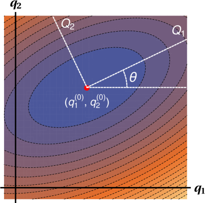
Figure 1: (Color online) Schematic representation of iso-potential curves of a mass-weighted potential in the 2-dimensional configuration space of lab-frame coordinates $\{q_{1},q_{2}\}$. These curves are ellipses centered at the moving equilibrium position $\left(q_{1}^{(0)},q_{2}^{(0)}\right)$ with the orientation of the principal axes given by the angle $\theta$. The dynamical normal mode coordinates $\{Q_{1},Q_{2}\}$ are translated from the origin but also rotated by $\theta$.

We have just shown that a condition to define independent modes by a point transformation is that $\theta$ (and therefore the transformation $A$) does not depend on time. What does this parameter represent?

Let us now visualize the mass-weighted symmetric potential $\widetilde{K}$ in Eq. (17) as a matrix defining a quadratic form. Quadratic forms are geometrically represented by conic sections. If $\widetilde{K}$ is positive definite (i. e., with positive eigenvalues), the conic section defined by $\widetilde{K}$ is an ellipse centered at the moving equilibrium position $\left(q_{1}^{(0)},q_{2}^{(0)}\right)$. These ellipses are iso-potential curves of the mass-weighted potential $\widetilde{K}$ in the $2$-dimensional configuration space $\{{q_{1},q_{2}\}}$, see Fig. 1. The principal axes theorem states that the orthonormal coordinate system where the ellipse is well-oriented is given by the orthonormal eigenvectors of $\widetilde{K}$, while the inverse of the square root of its eigenvalues are the radii of the corresponding axes. The orthogonal matrix (19) is formed by the eigenvectors of $\widetilde{K}$,

$$v_{1}^{T} = (\cos\theta,\sin\theta)$$

$$v_{2}^{T} = (-\sin\theta,\cos\theta).$$

These vectors define the orthonormal coordinate system where the ellipse is well-oriented, see Fig. 1. Therefore the parameter $\theta$ gives us the orientation of the ellipse. More generally, it gives the orientation of the principal axes if $\widetilde{K}$ is not positive (The engineering of fast dynamics may require that an eigenfrequency becomes transiently an imaginary number ChenPRL ). In general for a time dependent potential, the equilibrium position, the shape (size of principal axes) and orientation (angle $\theta$) will vary in time, but only the rotation of the principal axes couples the normal modes.

III Application to trapped-ion systems

In this section, we apply the results of the previous sections to systems of two ions in a linear trap, or one ion in a two dimensional trap. In particular we analyze if independent dynamical normal modes can be defined by point transformations. This is a key issue to design and engineer fast and robust protocols for operations needed to develop scalable quantum information processing: ion transport PTGM2013 ; PBGLM2014 ; LPRCM2015 , trap expansions or compressions PMAHM2015 , ion splitting PMPRM2015 , phase gates phaseg , or rotations PWGSM2016 .

III.1 Transport and expansions (or compressions) of two interacting trapped ions

Let us consider two singly-charged, positive ions in a linear trap at lab-frame coordinates $q_{1}$ and $q_{2}$, coupled via Coulomb interaction and trapped in an external, possibly time dependent, harmonic potential PBGLM2014 ; PMAHM2015 . The external potential can be translated PBGLM2014 and, in addition, expanded or compressed PMAHM2015 . The Hamiltonian describing this system is

$$H = \frac{p_{1}^{2}}{2m_{1}}+\frac{p_{2}^{2}}{2m_{2}}+U,$$

$$U = \frac{1}{2}\sum_{i=1}^{2}k(t)\left[q_{i}-Q_{0}(t)\right]^{2}+\frac{C_{c}}{q_{1}-q_{2}}.$$ (29)

Here, $C_{c}=\frac{e^{2}}{4\pi\epsilon_{0}}$ is the Coulomb constant and $k(t)$ is the common (time-dependent) spring constant that determines the oscillation frequency of each ion ($\omega_{i}^{2}=k/m_{i}$) in the absence of Coulomb coupling PMAHM2015 . $Q_{0}=Q_{0}(t)$ defines the position of the minimum of the external potential, i. e., the position of the, possibly moving, trap PBGLM2014 . We can also set $q_{1}>q_{2}$ because of the strong Coulomb repulsion PTGM2013 . If the ions are sufficiently cold, they “crystallize” around the classical equilibrium positions $q_{i}^{(0)}$, which are solutions of the set of equations $\frac{\partial U}{\partial q_{i}}=0$ for $i=1,2$,

$$q_{1}^{(0)} = Q_{0}+\left(\frac{C_{c}}{4k}\right)^{1/3}=Q_{0}+\frac{q_{0}}{2},$$

$$q_{2}^{(0)} = Q_{0}-\left(\frac{C_{c}}{4k}\right)^{1/3}=Q_{0}-\frac{q_{0}}{2},$$

where $q_{0}=q_{1}^{(0)}-q_{2}^{(0)}=(2C_{c}/k)^{1/3}$ is the equilibrium distance between ions. These positions are time dependent but independent of the mass, as we assume that the external potential is due to trap electrodes that interact only with the ionic charge. If we now approximate the coupling potential $U$ by its Taylor expansion truncated to second order in $q_{i}-q_{i}^{(0)}$ (small displacements from equilibrium), we end up with a quadratic potential. Therefore, up to a purely time dependent term, we can approximate the Hamiltonian (29) harmonically as

$$H = \frac{p_{1}^{2}}{2m_{1}}+\frac{p_{2}^{2}}{2m_{2}}$$ (30)

$$+ \frac{1}{2}\!\left(q_{1}\!-\!q_{1}^{(0)},q_{2}\!-\!q_{2}^{(0)}\right)K\left(\begin{matrix}q_{1}\!-\!q_{1}^{(0)}\\ q_{2}\!-\!q_{2}^{(0)}\end{matrix}\right)$$

with the $K$ matrix given by

$$K=\left(\begin{matrix}2k&-k\\ -k&2k\end{matrix}\right).$$

This Hamiltonian corresponds to the case $k_{1}=k_{2}=k$, so that Eq. (20) gives a constant $\theta$ even for a time-dependent $k$,

$$\tan 2\theta = \frac{\sqrt{m_{1}m_{2}}}{m_{1}-m_{2}}.$$ (31)

The normal modes are given by (25)

$$\!\!\left(\!\begin{matrix}Q_{1}\\ Q_{2}\end{matrix}\!\right)=\left(\!\begin{matrix}\sqrt{m_{1}}\cos\theta&\sqrt{m_{2}}\sin\theta\\ -\sqrt{m_{1}}\sin\theta&\sqrt{m_{2}}\cos\theta\end{matrix}\right)\!\left(\!\begin{matrix}q_{1}\!-\!\left(Q_{0}+q_{0}/2\right)\\ q_{2}\!-\!\left(Q_{0}-q_{0}/2\right)\end{matrix}\right)\!,$$

with $\theta$ given by relation (31). These normal modes depend on time through the time dependent parameters $Q_{0}$ and $q_{0}$. In these coordinates, the Hamiltonian (30) transforms to the diagonal and uncoupled form (28),

$$\widetilde{H} = \frac{1}{2}\sum_{i=1}^{2}\left(P_{i}^{2}+\Omega_{i}^{2}Q_{i}^{2}\right)-(P_{1},P_{2})A\left(\begin{matrix}\dot{Q}_{0}+\dot{q}_{0}/2\\ \dot{Q}_{0}-\dot{q}_{0}/2\end{matrix}\right),$$

where

$$\Omega_{1}^{2} = k\left(\frac{2\cos^{2}\theta}{m_{1}}+\frac{2\sin^{2}\theta}{m_{2}}-\frac{\sin 2\theta}{\sqrt{m_{1}m_{2}}}\right),$$

$$\Omega_{2}^{2} = k\left(\frac{2\sin^{2}\theta}{m_{1}}+\frac{2\cos^{2}\theta}{m_{2}}+\frac{\sin 2\theta}{\sqrt{m_{1}m_{2}}}\right),$$ (33)

which may depend on time because of $k=k(t)$. Note that the inertial effects in this Hamiltonian (LABEL:H_tilde_transport) are only included into the linear-in-momentum term and are due to the transport of the trap ($\dot{Q}_{0}$ term) and/or expansion or compression of the trap ($\dot{q}_{0}$ term). Geometrically the center of the ellipses in Fig. 1 can move in the $\{q_{1},q_{2}\}$ plane, and the size may change as well, but the orientation remains constant in time.

III.2 Separation of two trapped interacting ions

Figure 2: (Color online) Scheme of the separation of two ions, from an external harmonic potential to a double well.

Consider now the problem of separating (or recombining) two interacting trapped ions as in PMPRM2015 , see Fig. 2. The Hamiltonian of a system of two ions of masses $m_{1}$ and $m_{2}$ and charge $e$ located at $q_{1}>q_{2}$ in the laboratory frame is

$$H = \frac{p_{1}^{2}}{2m_{1}}+\frac{p_{2}^{2}}{2m_{2}}+U,$$

$$U = \alpha(t)(q_{1}^{2}+q_{2}^{2})+\beta(t)(q_{1}^{4}+q_{2}^{4})+\frac{C_{c}}{q_{1}-q_{2}},$$

where $\alpha(t)$ and $\beta(t)$ are time dependent functions PMPRM2015 . Typically $\alpha(0)>0$, $\beta(0)=0$, whereas at final time $\beta(t_{f})>0$, $\alpha(t_{f})<0$ to implement an evolution from a harmonic trap to a double well, see Fig. 2.

To set a quadratic (approximate) Hamiltonian we proceed as in the previous sub-section: first, we obtain the equilibrium positions $q_{i}^{(0)}$ of each ion by minimizing the potential $U$ and then expand the potential $U$ to second order in $q_{i}-q_{i}^{(0)}$. If the equilibrium positions are denoted by $q_{1}^{(0)}=q_{0}/2$ and $q_{2}^{(0)}=-q_{0}/2$ (with $q_{0}$ being the equilibrium distance between ions) this procedure gives the quadratic Hamiltonian

$$H = \frac{p_{1}^{2}}{2m_{1}}+\frac{p_{2}^{2}}{2m_{2}}$$

$$+ \frac{1}{2}\left(q_{1}-q_{1}^{(0)},q_{2}-q_{2}^{(0)}\right)K\left(\begin{matrix}q_{1}-q_{1}^{(0)}\\ q_{2}-q_{2}^{(0)}\end{matrix}\right),$$

with a $K$ matrix given by

$$k_{1} = k_{2}=2\alpha+3\beta q_{0}^{2}=k_{0},$$

$$k = \frac{2C_{c}}{q_{0}^{3}},$$

and where the equilibrium distance between ions $q_{0}=q_{1}^{(0)}-q_{2}^{(0)}$ is the solution of the quintic equation PMPRM2015 ; HS2006

$$\beta q_{0}^{5}+2\alpha q_{0}^{3}-2C_{c}=0.$$ (34)

In this case

$$\tan 2\theta = \frac{\sqrt{m_{1}m_{2}}}{m_{1}-m_{2}}\left(\frac{4C_{c}}{2\alpha q_{0}^{3}+3\beta q_{0}^{5}+2C_{c}}\right),$$ (35)

which, in general, depends on time. In principle, there are two ways to end up with a time-independent $\theta$ for time dependent $\alpha$ and $\beta$:

• Equal masses, $m_{1}=m_{2}$, for which $\theta=\pm\pi/4$ regardless of the time dependence of $\alpha$ and $\beta$ PMPRM2015 .

• $\alpha$ and $\beta$ linked by

  $$\frac{\beta^{3}}{\alpha^{5}}=\textrm{constant},$$ (36)

  regardless of the masses. This implies that the products $\beta q_{0}^{5}$ and $\alpha q_{0}^{3}$ are constants. The particular case $\beta=0$ corresponds to the one considered in the previous subsection (transport and expansions). The case $\beta\neq 0$ is interesting as it allows to separate or approach the two ions by decreasing or increasing $\alpha<0$ and $\beta>0$ according to Eq. (36), i.e., in a double well confining potential throughout the process.

III.3 Phase gates

A phase gate can be implemented by applying well designed time-dependent forces that depend on the internal states of the two ions in a linear trap phaseg . The external harmonic trap for each ion has a fixed spring constant $k_{0}$. For a particular spin configuration the Hamiltonian becomes

$$H = \frac{p_{1}^{2}}{2m_{1}}+\frac{p_{2}^{2}}{2m_{2}}+\frac{1}{2}k_{0}(q_{1}^{2}+q_{2}^{2})+\frac{C_{c}}{q_{1}-q_{2}}$$ (37)

$$+ F_{1}(t)q_{1}+F_{2}(t)q_{2}.$$

Equilibrium positions and the equilibrium distance between the ions are

$$q_{1}^{(0)} = \frac{B-2k_{0}^{2}\Delta(F_{2}+2F_{1})}{6k_{0}^{3}\Delta},$$

$$q_{2}^{(0)} = \frac{-B-2k_{0}^{2}\Delta(F_{1}+2F_{2})}{6k_{0}^{3}\Delta},$$

$$q_{0} = q_{1}^{(0)}-q_{2}^{(0)}=\frac{2B-2k_{0}^{2}\Delta(F_{1}+F_{2})}{6k_{0}^{3}\Delta},$$

where

$$B = (F_{1}-F_{2})^{2}k_{0}^{4}+\Delta^{2},$$

$$\Delta = \bigg{\{}-(F_{1}-F_{2})^{3}k_{0}^{6}+27C_{c}k_{0}^{8}$$

$$+ 3\sqrt{3C_{c}k_{0}^{14}[-2(F_{1}-F_{2})^{3}+27C_{c}k_{0}^{2}]}\bigg{\}}^{1/3}.$$

This leads to a $K$ matrix with

$$k=\frac{2C_{c}}{q_{0}^{3}},\;\;\;\;\;k_{1}=k_{2}=k_{0},$$

so that

$$\tan 2\theta=\frac{\sqrt{m_{1}m_{2}}}{m_{1}-m_{2}}\,\frac{4C_{c}}{k_{0}q_{0}^{3}+2C_{c}}.$$

The angle $\theta$ is in general time-dependent, but it becomes constant in some cases, specifically for $m_{1}=m_{2}$, and also for $F_{1}=F_{2}$. This latter case in fact reduces to the transport of two ions considered before. For different masses and forces the ellipsoid rotates so that the modes $Q_{1},\,Q_{2}$ are coupled. A way out, if the forces are small so that the linear term in Eq. (37) may be considered a perturbation, is to define the modes for Juanjo

$$H_{0}=\frac{p_{1}^{2}}{2m_{1}}+\frac{p_{2}^{2}}{2m_{2}}+\frac{1}{2}k_{0}(q_{1}^{2}+q_{2}^{2})+\frac{C_{c}}{q_{1}-q_{2}}.$$

These zeroth order modes, $Q_{1}(F_{j}=0),\,Q_{2}(F_{j}=0)$, $j=1,2$, are of course uncoupled since all coefficients in $H_{0}$ are time independent. $H_{0}$ may thus be easily diagonalized. Specifically, all the $K$ matrix coefficients become equal, $\tan 2\theta=\frac{\sqrt{m_{1}m_{2}}}{m_{1}-m_{2}}$, and the equilibrium positions simplify to the constant values $\pm[\frac{C_{c}}{4k_{0}}]^{1/3}$. The inverse transformation of Eq. (25) for these zeroth order modes,

$$\left(\begin{matrix}q_{1}\\ q_{2}\end{matrix}\right)=\left(\begin{matrix}q_{1}^{(0)}\\ q_{2}^{(0)}\end{matrix}\right)_{\!\!F_{j}=0}+A_{F_{j}=0}^{\!-1}\!\left(\begin{matrix}Q_{1}\\ Q_{2}\end{matrix}\right)_{\!\!F_{j}=0},$$

enables us to write the perturbative linear terms in $H$ in terms of the uncoupled modes, so that $H$ is approximated as a sum of two uncoupled Hamiltonians Juanjo ; phaseg .

III.4 Anisotropic harmonic oscillator in 2D with rotation

Consider now a single particle of mass $m$ trapped in a 2D anisotropic harmonic oscillator which is rotating around the $z$ axis with angular velocity $\dot{\varphi}$ Masuda . Let us denote by $q_{1}=x$ and $q_{2}=y$ the lab frame coordinates of the ion, and by

$$\tilde{q}_{1}(t) = q_{1}\cos\varphi(t)+q_{2}\sin\varphi(t),$$

$$\tilde{q}_{2}(t) = -q_{1}\sin\varphi(t)+q_{2}\cos\varphi(t).$$ (38)

the coordinates in the rotating frame. The Hamiltonian in the lab frame is given by

$$H = \frac{p_{1}^{2}}{2m}+\frac{p_{2}^{2}}{2m}+\frac{1}{2}m\sum_{i=1}^{2}\omega_{i}^{2}\tilde{q}_{i}(q_{1},q_{2};t)^{2},$$

where $\omega_{1}\neq\omega_{2}$ are the angular frequencies along the rotating principal axes. (Note that for the trivial isotropic case $\omega_{1}=\omega_{2}$ the Hamiltonian is already uncoupled in the laboratory frame.) $H$ can be written as

$$H=\frac{p_{1}^{2}}{2m}+\frac{p_{2}^{2}}{2m}+\frac{1}{2}(q_{1},q_{2})K\left(\begin{matrix}q_{1}\\ q_{2}\end{matrix}\right),$$ (39)

with the $K$ matrix given by

$$k_{1} = m\left(\omega_{1}^{2}\cos^{2}\varphi+\omega_{2}^{2}\sin^{2}\varphi\right)-k,$$

$$k_{2} = m\left(\omega_{1}^{2}\sin^{2}\varphi+\omega_{2}^{2}\cos^{2}\varphi\right)-k,$$

$$k = -\frac{m}{2}(\omega_{1}^{2}-\omega_{2}^{2})\sin 2\varphi.$$

Unlike the previous operations, there is no need to make the harmonic approximation around the equilibrium since $H$ is already quadratic. Moreover $q_{1}^{(0)}=q_{2}^{(0)}=0$ and, quite simply, $\theta=\varphi$. The Hamiltonian $\tilde{H}$ takes the form in Eq. (LABEL:H_tilde_general) without the linear term and with $\Omega_{i}=\omega_{i}$, and $Q_{i}=\sqrt{m}\widetilde{q}_{i}$, i.e., the normal mode coordinates are the (mass-weighted) rotating coordinates in Eq. (38), coupled by the angular momentum term $-\dot{\theta}L_{z}$. We conclude that the 2D anisotropic problem is not separable by means of a linear point transformation of coordinates.

Making use of an additional physical interaction, it is possible to cancel the coupling term so that the resulting Hamiltonian is diagonal. Specifically, if the particle is an ion of (positive) charge $e$, a homogeneous magnetic field $-B\hat{z}$ introduces, in the rotating frame, the diamagnetic and paramagnetic terms, see e.g. hami ,

$$\frac{1}{2}\omega_{L}^{2}(Q_{1}^{2}+Q_{2}^{2})+\omega_{L}L_{z},$$

where the Larmor frequency is $\omega_{L}=eB/(2m)$. (This term is invariant with respect to rotations around $\hat{z}$, so that it has the same form in laboratory coordinates and momenta.) Adjusting the magnetic field to exactly cancel $-\dot{\theta}L_{z}$ with $\omega_{L}=\dot{\theta}$, provides an uncoupled normal-mode Hamiltonian with time dependent frequencies $[\omega_{i}^{2}+\omega_{L}^{2}]^{1/2}$. Note that the harmonic 2D potential complemented by a confining term in $z$-direction cannot be purely electrostatic as it would not obey Laplace’s equation Masuda . It could however be created by other means, for example as an effective pondermotive potential.

III.4.1 Compressions and expansions

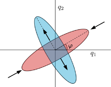
Figure 3: (Color online) Compression and expansion along the non rotating principal axes of a 2D anisotropic oscillator amounts to a $\pi/2$ rotation of the potential

We have pointed out before that $k=0$, with $k_{1}$ and $k_{2}$ time-dependent leads to a constant $\theta$ and independent modes. For a single particle in a harmonic potential, this corresponds to time-dependent frequencies (expansions and compressions) along the nonrotating principal axes of the potential. Specific orthogonal compressions and expansions where the two normal mode frequencies interchange, amount at final time to a $\frac{\pi}{2}$-rotation of the potential, see Fig. 3, although the process itself is different. Slow adiabatic expansion and compression processes would connect initial and final excited energy levels differently from a true rotation, which may be important for inverse engineering operations. In the slow frequency manipulation the levels cross, so that their energy ordering changes. Take for example the initial states with vibrational quantum numbers 01 and 10 for the principal directions 1 and 2 and such that $\omega_{1}<\omega_{2}$. Then the energies satisfy initially $E_{01}>E_{10}$. If the values of the frequencies are interchanged along the process the energies also switch, $E_{10}>E_{10}$. On the contrary, a slow true rotation does not produce crossings and energy reordering.

IV Discussion

Motivated by the need to inverse engineer the dynamics of trapped ions and other systems in the small oscillations regime, we have studied the possibility to define, via linear point transformations, independent dynamical normal modes for two dimensional systems under time-dependent external control. Whereas the analysis of further dimensions is certainly worthwhile, note the physical relevance of two dimensions, as they suffice to describe pairs of ions in linear traps, and universal quantum computing may be achieved by combining operations on one and two qubits. We also expect that the results found here may set a useful guide for further dimensions. The condition that determines the coupling of the modes turns out to be the rotation of the harmonic potential in the (laboratory) 2D coordinate space. Nonrotating potentials lead to uncoupled dynamical modes. Different examples have been analyzed and in some of them ways to avoid the coupling have been pointed out: by a specific design of the time dependence of the control parameters in separation operations, by adding compensating terms in the Hamiltonian in rotations, or perturbatively in phase gates. Point transformations are the ones used for time-independent normal-mode analysis, so they are a natural choice. Moreover they are easy to understand, visualize, and implement. More general (mixed) canonical transformations have not been considered in this paper, but they are in principle possible Inva ; Manko ; Ji ; Xu ; AbdallaLeach ; Menouar and will be discussed elsewhere. Generically their physical meaning, definition, and practical use become more involved, so only simplified potential configurations and dynamics are typically worked out explicitly Inva ; Manko ; Ji ; Xu ; AbdallaLeach ; Menouar .

Appendix A Derivation of the Hamiltonian of the spring system

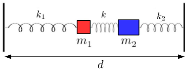
Figure 4: (Color online) Mechanical system of two masses connected to each other and to the walls by springs with time-dependent spring “constants”. This system is found to be mathematically equivalent to many of the trapped ions systems considered throughout the text.

In this Appendix we find the Hamiltonian describing the dynamics of two masses connected by springs as illustrated in Fig. 4. The three springs are assumed to have zero natural length but time-dependent spring “constants”. If $q_{i}$ is the lab frame coordinate of $m_{i}$ measured from the fixed left wall, the Hamiltonian is given by

$$H = \frac{p_{1}^{2}}{2m_{1}}+\frac{p_{2}^{2}}{2m_{2}}+U$$

$$U = \frac{1}{2}k_{1}q_{1}^{2}+\frac{1}{2}k_{2}\left(d-q_{2}\right)^{2}+\frac{1}{2}k(q_{2}-q_{1})^{2},$$

where $p_{i}$ is the conjugate momentum of the coordinate $q_{i}$. By solving the set of equations $\partial_{q_{i}}U=0$ for $i=1,2$ we find the equilibrium positions of the two connected masses at

$$q_{1}^{(0)} = q_{0}\left(\frac{k}{k_{1}}\right),$$

$$q_{2}^{(0)} = q_{1}^{(0)}+q_{0},$$

where $q_{0}=q_{2}^{(0)}-q_{1}^{(0)}$, the equilibrium distance between masses, is given by

$$q_{0} = d\left[\frac{k_{1}k_{2}}{k_{1}k_{2}+k(k_{1}+k_{2})}\right].$$

The equilibrium positions are generally moving, they depend on time because of the time dependence of $k,\,k_{1}$, and $k_{2}$. We can now expand the coupling potential $U$ around its equilibrium position (small oscillations), and up to a purely time dependent function, we have

$$U = \frac{1}{2}\!\left(q_{1}\!-\!q_{1}^{(0)},q_{2}\!-\!q_{2}^{(0)}\right)\left(\begin{matrix}k_{1}+k&-k\\ -k&k_{2}+k\end{matrix}\right)\left(\begin{matrix}q_{1}\!-\!q_{1}^{(0)}\\ q_{2}\!-\!q_{2}^{(0)}\end{matrix}\right),$$

where the $q_{i}-q_{i}^{(0)}$ measure the displacement of mass $m_{i}$ from its (moving) equilibrium position. The full Hamiltonian then may be written exactly as in Eq. (6).

Appendix B Quantum treatment

The results in the main text regarding the form of the Hamiltonians and transformations can be used directly in quantum mechanical systems. The starting point is the 2D time dependent Schrödinger equation

$$i\hbar\partial_{t}\psi(q_{1},q_{2};t)=H(q_{1},q_{2};t)\psi(q_{1},q_{2};t),$$ (40)

with $H(q_{1},q_{2};t)$ given in Eq. (2). Let us now consider the use of the new coordinates (8) and define

$$\Psi=\Psi(Q_{1},Q_{2};t)\equiv\psi[q_{1}(Q_{1},Q_{2};t),q_{2}(Q_{1},Q_{2};t);t].$$ (41)

We now calculate the time derivative of the transformed wavefunction taking into account the time dependences separately and applying the chain rule,

$$i\hbar\partial_{t}\Psi = i\hbar\partial_{t}\psi[q_{1}(Q_{1},Q_{2};t),q_{2}(Q_{1},Q_{2};t);t]$$ (42)

$$= i\hbar\left[\partial_{t}+\partial_{t}q_{1}\partial_{q_{1}}+\partial_{t}q_{2}\partial_{q_{2}}\right]\Psi$$

$$= \left[H(Q_{1},Q_{2})-(p_{1},p_{2})\left(\begin{matrix}\partial_{t}q_{1}\\ \partial_{t}q_{2}\end{matrix}\right)\right]\Psi,$$

with $p_{j}=-i\hbar\partial_{q_{j}}$. The first term is just the transformed Hamiltonian, i. e., the original Hamiltonian written in the new coordinates with the usual definition $P_{j}=-i\hbar\partial_{Q_{j}}$, and the second term is an inertial contribution due to the time dependence of the transformation. It is now clear that the effective Hamiltonian is

$$\widetilde{H}(Q_{1},Q_{2}) = H(Q_{1},Q_{2})-(P_{1},P_{2})A\left(\begin{matrix}\partial_{t}q_{1}\\ \partial_{t}q_{2}\end{matrix}\right),$$ (43)

where relation (10) has been used to write the old momenta in terms of the new ones. The explicit time derivative of the $q_{i}$ coordinates in (43) can be calculated directly by inverting transformation (8),

$$\left(\begin{matrix}\partial_{t}q_{1}\\ \partial_{t}q_{2}\end{matrix}\right)=\left(\begin{matrix}\dot{q}_{1}^{(0)}\\ \dot{q}_{2}^{(0)}\end{matrix}\right)+\partial_{t}(A^{-1})\left(\begin{matrix}Q_{1}\\ Q_{2}\end{matrix}\right),$$ (44)

which leads finally to an effective Hamiltonian

$$\widetilde{H} = H-(P_{1},P_{2})A\left(\begin{matrix}\dot{q}_{1}^{(0)}\\ \dot{q}_{2}^{(0)}\end{matrix}\right)-(P_{1},P_{2})A\partial_{t}(A^{-1})\left(\begin{matrix}Q_{1}\\ Q_{2}\end{matrix}\right)$$ (45)

$$= H-(P_{1},P_{2})A\left(\begin{matrix}\dot{q}_{1}^{(0)}\\ \dot{q}_{2}^{(0)}\end{matrix}\right)-\dot{\theta}\left(Q_{1}P_{2}-Q_{2}P_{1}\right),$$

where, for writing the last term, we have used the relation

$$A\partial_{t}(A^{-1})=\dot{\theta}\left(\begin{matrix}0&-1\\ 1&0\end{matrix}\right).$$ (46)

The effective Hamiltonian when using transformed coordinates thus takes exactly the same form as in classical mechanics, Eq. (LABEL:H_tilde_general).

References

• (1) J. I. Cirac and P. Zoller, Phys. Rev. Lett. 74, 4091 (1995).
• (2) A. M. Steane Appl. Phys. B 64 623 (1997).
• (3) D. V. F. James, Appl. Phys. B 66 181 (1998).
• (4) G. Morigi and H. Walther, Eur. Phys. J. D 13, 261 (2001).
• (5) J. P. Home, D. Hanneke, J. D. Jost, D. Leibfried and D. J. Wineland, New J. Phys. 13, 073026 (2011).
• (6) H. Landa, M. Drewsen, B. Reznik, and A. Retzker, New, J. Phys. 14, 093023 (2012).
• (7) H. Landa, M. Drewsen, B. Reznik, and A Retzker, J. Phys. A: Math. Theor. 45, 455305 (2012).
• (8) M. Palmero, E Torrontegui, D. Guéry-Odelin, and J. G. Muga, Phys. Rev. A 88, 053423 (2013).
• (9) M. Palmero, R. Bowler, J. P. Gaebler, D. Leibfried, J. G. Muga Phys. Rev. A 90, 053408 (2014).
• (10) M. Palmero, S. Martínez-Garaot, J. Alonso, J. P. Home, and J. G. Muga, Phys. Rev. A 91, 053411 (2015).
• (11) M. Palmero, S. Martínez-Garaot, U. G. Poschinger, A. Ruschhaupt, and J. G. Muga, New J. Phys.17, 093031 (2015).
• (12) X. J. Lu, M. Palmero, A. Ruschhaupt, X. Chen, and J. G. Muga, Physica Scripta 90, 974038 (2015).
• (13) M. Palmero, S. Wang, D. Guéry-Odelin, Jr-Shin Li, and J G Muga, New J. Phys. 18, 043014 (2016).
• (14) M. Palmero, S. Martínez-Garaot, D. Leibfried, D. J. Wineland, and J. G. Muga, arXiv: 1609.01892.
• (15) D. J. Wineland, C. Monroe, W. M. Itano, D. Leibfried, B. E. King, and D. M. Meekhof, J. Res. Natl. Inst. Stand. Technol. 103, 259 (1998).
• (16) D. Kielpinski, C. Monroe, and D. J.Wineland, Nature 417, 709 (2002).
• (17) H. Goldstein, C. Poole, J, Safko, Classical Mechanics, 3rd Ed, Addison-Wesley (2001)
• (18) X. Chen, A. Ruschhaupt, S. Schmidt, A. del Campo, D. Guéry-Odelin, and J. G. Muga, Phys. Rev. Lett. 104, 063002 (2010).
• (19) W. Dittrich, M. Reuter, Classical and Quantum Dynamics, Springer (2001).
• (20) J. P. Home and A. M. Steane, Quantum Inf. Comput. 6, 289 (2006).
• (21) J. J. García-Ripoll, P. Zoller, and J. I. Cirac, Phys. Rev. A 71, 062309 (2005).
• (22) S. Masuda and S. A. Rice, J. Phys. Chem. B 119 11079 (2015).
• (23) M. G. Calkin, Lagrangian and Hamiltonian mechanics: Solutions to the exercises (World Scientific, Singapore, 1999)
• (24) V. V. Dodonov and V. I. Man ko, Invariants and Evolution of Non-stationary Quantum Systems, in Proc. P. N. Lebedev Physical lnstitute 183, ed. by M. A. Markov (Commack, N. Y., Nova Science, 1987)
• (25) F. Leyvraz, V. I. Manko, T. H. Seligman, Phys. Lett. A 2010, 26 (1996).
• (26) J.-Y. Ji and J. Hong, J. Phys. A: Math. Gen. 31, L689 (1998).
• (27) X.-W. Xu, J. Phys. A: Math. Gen. 33, 2447 (2000).
• (28) M. S. Abdalla and P. G. Leach, J. Phys. A: Math. Gen. 38, 881 (2005).
• (29) S. Menouar, M. Maamache, and J. R. Choi, Annals of Phys. 325, 1708 (2010).