Two-electron bound states near a Coulomb impurity in gapped graphene

Abstract

We formulate and solve the perhaps simplest two-body bound state problem for interacting Dirac fermions in two spatial dimensions. A two-body bound state is predicted for gapped graphene monolayers in the presence of weakly repulsive electron-electron interactions and a Coulomb impurity with charge $Ze>0$, where the most interesting case corresponds to $Z=1$. We introduce a variational Chandrasekhar-Dirac spinor wave function and show the existence of at least one bound state. This state leaves clear signatures accessible by scanning tunneling microscopy. One may thereby obtain direct information about the strength of electron-electron interactions in graphene.

I Introduction

Ever since the Nobel prize winning experiments by the Manchester group in 2004 geim2004 ; geim2005 , two-dimensional (2D) graphene monolayers continue to attract a lot of attention. Besides graphene’s application potential, much of the interest comes from the fact that low-energy fermionic quasiparticles in graphene are governed by the 2D Dirac Hamiltonian rmp1 ; goerbig ; philip ; eva ; kotov ; miransky . As a consequence, typical effects predicted by relativistic quantum mechanics and/or quantum electrodynamics can be studied in table-top experiments. Recent progress has demonstrated that one can reach the ballistic (disorder-free) regime Kim2016 , e.g., by encapsulating the graphene layer in boron nitride crystals boron . We will therefore not consider disorder effects in this work.

Here we address the perhaps simplest interacting problem for relativistic fermions by considering a gapped graphene monolayer subject to relatively weak (screened) Coulomb interactions and in the presence of a single Coulomb impurity. A band gap $2\Delta$ in the Dirac fermion spectrum may be caused by a variety of mechanisms, e.g., by strain engineering vozmediano , spin-orbit coupling kanemele2005 ; huertas , substrate-induced superlattices ponomarenko ; song , or simply as finite-size effect in a ribbon geometry rmp1 . The Coulomb interaction strength is customarily quantified in terms of the effective fine-structure constant

$$\alpha=\frac{e^{2}}{\kappa\hbar v_{F}}\simeq\frac{2.2}{\kappa},$$ (1)

where $\kappa$ is a dielectric constant due to the surrounding substrate and $v_{F}\simeq 10^{6}$ m$/$s denotes the Fermi velocity kotov . The estimate in Eq. (1) follows with $c/v_{F}\simeq 300$ and $e^{2}/(\hbar c)\simeq 1/137$. The value of $\alpha$ thus depends on the choice of gating geometry and the ensuing screening effects. As explained below, the weak interaction regime where our theory is applicable is defined by $\alpha\lesssim 0.4$. In this regime, we find that a pair of repulsively interacting Dirac fermions subject to the attractive potential of a Coulomb impurity with charge $Ze$ will form a two-body bound state localized near the impurity. We mainly focus on the most interesting case $Z=1$, but also comment on what happens for $Z>1$.

The signatures of the predicted bound state could be observed by means of scanning tunnelling microscopy (STM) experiments similar to those previously reporting supercritical behavior in graphene crommie1 ; luican ; crommie2 and trapped electron states in electrostatically defined graphene dots Lee2016 ; Gutierrez . An experimental observation of the predicted two-body bound state could therefore probe and quantify Coulomb interaction effects. In order to consistently formulate this relativistic quantum-mechanical two-particle problem, it is necessary to stay away from the supercritical instability rmp1 ; kotov ; novikov ; gamayun , otherwise one inevitably has to face a complicated many-body problem kotov . For small values of $\alpha$, supercriticality is absent, and as explained below, a two-particle bound state exists. We mention in passing that the two-body problem in graphene has also been studied in Refs. guinea ; terekhov ; koch ; ziegler ; entin ; gaul ; shytov ; portnoi . In contrast to our work, however, those papers considered translationally invariant settings without Coulomb impurity. Similar problems (again without Coulomb impurity) have also been analyzed in the context of Dirac excitons in single-layer transition-metal dichalcogenides rodin ; zhong ; trushin .

The negatively charged two-electron hydrogen ion $H^{-}$ represents a classic problem of nonrelativistic quantum mechanics chandrasekhar ; bethe ; hill ; bransden ; andersen ; sorba . In particular, it is well known hill that $H^{-}$ has a single bound state in three spatial dimensions. The simplest way to prove its stability is to demonstrate the existence of a variational wave function with energy below the ground-state energy of the hydrogen atom. Interestingly, it is impossible to achieve this task with a factorized wave function sorba . The simplest way to construct a variational wave function for the ground state of $H^{-}$ is due to Chandrasekhar chandrasekhar . With $r_{l=1,2}=|{\bf r}_{l}|$ denoting the distance of the respective electron from the proton, the Chandrasekhar ansatz for the spatial part of the two-particle wave function, $\Psi({\bf r}_{1},{\bf r}_{2})$, contains two variational parameters ($a,b$) and is (up to a normalization factor) given by

$$\Psi({\bf r}_{1},{\bf r}_{2})=e^{-ar_{1}-br_{2}}-\epsilon e^{-br_{1}-ar_{2}},$$ (2)

where $\epsilon=\mp 1$ corresponds to a spin singlet/triplet state, respectively. Here the important insight is that $a$ and $b$ are not required to be identical. Indeed, the minimal variational energy for a two-body bound state is obtained for $a\neq b$ in the spin singlet configuration ($\epsilon=-1$). Improved variational energy estimates can be obtained by taking into account the dependence on the relative distance $r_{12}=|{\bf r}_{1}-{\bf r}_{2}|$ in Eq. (2), e.g., through a correlation factor of the form $(1+c\,r_{12})$ sorba . Since the inclusion of such a factor is technically cumbersome yet not expected to cause qualitative changes, cf. Ref. sorba , we here restrict ourselves to uncorrelated wave functions and leave the analysis of correlation effects to future work.

The nonrelativistic hydrogen ion has also been studied for the 2D case. For instance, the so-called $D^{-}$ problem describes a donor impurity ion with two attached electrons in a 2D semiconductor quantum well phelps ; louie ; larsen92a ; larsen92b ; sandler ; ivanov . Interesting experimental results on the $D^{-}$ problem have appeared in Ref. etienne , where effects of quantum confinement on two-body bound-state energies have been studied. In the absence of a magnetic field, only a single bound state in the spin singlet sector is expected again. We note in passing that the $D^{-}$ problem is also similar to the negatively charged exciton ($X^{-}$) problem, which was experimentally studied in quantum wells pepper .

In this paper, we turn to the 2D relativistic counterpart of the above system, which is realizable in gapped graphene monolayers (or topological insulator surfaces) containing a Coulomb impurity. The corresponding relativistic $H^{-}$ problem is more difficult to define (and solve) because the single-particle Dirac Hamiltonian is unbounded from below brown ; talman ; nakatsuji . It then appears at first sight as if two-particle states of arbitrarily low energy can be generated by electron-electron interactions. As discussed below, in order to avoid this spurious and ultimately unphysical effect, it is necessary to employ a projection scheme which defines a mathematically clean framework. Such a projection scheme can be devised for interacting Dirac fermions in graphene if (i) a single-particle gap exists ($\Delta>0$), and (ii) electron-electron interactions are weak, see Refs. sucher1 ; sucher2 ; haeusleregger ; Egger .

The structure of the remainder of this article is as follows. We introduce the Dirac-Coulomb model and the appropriate projection scheme in Sec. II, followed by a discussion of the variational approach to the two-body bound state problem in Sec. III. (Details have been delegated to two appendices.) To that end, we formulate a Chandrasekhar-Dirac spinor ansatz generalizing Eq. (2) to the relativistic case. We evaluate all needed matrix elements and discuss the variational bound-state energy as a function of $\alpha$. In particular, we show variational estimates for the energy of the bound state in the presence of a standard Dirac mass term causing a band gap, assuming a spin-singlet state and impurity charge $Z=1$. We then turn to generalizations in Sec. IV, where we shall address (i) what happens for impurity charge $Z>1$, (ii) the effects of a topologically nontrivial band gap as obtained, e.g., from spin-orbit coupling effects, and (iii) the role of the valley state of each quasiparticle. In Sec. V, we address the observable consequences of the two-body bound state accessible to STM experiments. Finally, we offer some conclusions in Sec. VI.

II Dirac-Coulomb Model

We model the interacting two-particle problem for a gapped graphene monolayer in the presence of a charge impurity by the (properly projected, see below) Dirac-Coulomb Hamiltonian

$$H=\sum_{l=1,2}H_{\rm D}(l)+V_{\rm 2b}.$$ (3)

Here $H_{\rm D}(l)$ is the usual single-particle massive Dirac-Weyl Hamiltonian for particle $l=1,2$,

$$H_{\rm D}(l)=H_{0}(l)+H_{\rm gap}(l)+V_{\rm 1b}(l),$$ (4)

with kinetic part (the index $l$ being understood) rmp1

$$H_{0}=v_{F}(\tau_{z}\sigma_{x}p_{x}+\sigma_{y}p_{y}),$$ (5)

where Pauli matrices $\bm{\tau}$ ($\bm{\sigma}$) act in valley (sublattice) space and the momentum operator is ${\bf p}=-i\hbar\nabla$. With the dielectric constant $\kappa$, see Eq. (1), the single-particle potential

$$V_{\rm 1b}=-\frac{Ze^{2}}{\kappa r}=-\frac{Z\alpha\hbar v_{F}}{r}$$ (6)

describes a charge-$Z$ impurity at the origin. We mainly focus on the most interesting case of unit charge, $Z=1$, but comment on the case $Z>1$ in Sec. IV.1. In $H_{\rm D}$, we also include the term

$$H_{\rm gap}=\Delta\sigma_{z},$$ (7)

which results in a topologically trivial band gap of size $2\Delta$ rmp1 . However, it is straightforward to generalize our analysis to the case of a spin- and valley-dependent topological band gap, e.g., due to an intrinsic spin-orbit coupling mechanism kanemele2005 ; huertas ,

$$H_{\rm so}=\Delta\sigma_{z}\tau_{z}s_{z},$$ (8)

where $\bm{s}$ are Pauli matrices in spin space, see Sec. IV.2. Note that $H_{\rm gap}$ has the same sign for both spin projections while $H_{\rm so}$ has opposite sign.

The operator $H_{\rm D}$ is Hermitian only for $Z<Z_{\rm crit}=1/(2\alpha)$. Indeed, the lowest single-particle bound-state energy becomes imaginary for $Z>Z_{\rm crit}$, see Eq. (57) in App. A. We note that by regularizing the $r\to 0$ singularity of the Coulomb potential, the threshold shifts to a larger value $\tilde{Z}_{\rm crit}$, which weakly depends on the precise regularization prescription gamayun . Even in the regularized scheme, however, Hermiticity is lost for $Z>\tilde{Z}_{\rm crit}$. In the latter regime, bound states of the regularized Hamiltonian $\tilde{H}_{\rm D}$ dive into the negative part of the continuum spectrum ($E<-\Delta$) one by one, and thereby become quasi-stationary states, see Ref. gamayun . As remarked in Sec. I, one then necessarily has to consider the full many-body problem for $Z>\tilde{Z}_{\rm crit}$. For this reason, we will restrict ourselves to the weak-coupling regime. Moreover, for the sake of transparency, we focus on the narrower range $Z<1/(2\alpha)$, where no need for regularization arises and the exact Dirac-Coulomb wave functions summarized in App. A can be used. For the most interesting case $Z=1$, this implies that our theory is at best applicable for $\alpha<1/2$.

Since $H_{\rm D}$ is diagonal in valley and spin space, we can always choose a factorized form for the single-particle wave functions,

$$\Psi_{\tau,s}(x,y)=\Psi(x,y)|\tau,s\rangle,$$ (9)

where $\Psi(x,y)$ refers to the spatial part (including sublattice space), and $|\tau,s\rangle$ with $\tau=K/K^{\prime}=\pm 1$ and $s=\uparrow/\downarrow=\pm 1$ denotes the eigenstates of the operator $\tau_{z}s_{z}$. For an eigenstate $\Psi_{\tau,s}$ of $H_{\rm D}$ with energy $E$, the symmetry relations

$$\sigma_{y}\Psi_{\tau,s}^{*}=\Psi_{\tau,-s},\quad\sigma_{y}\Psi_{\tau,s}=\Psi_{-\tau,s},\quad\Psi_{\tau,s}^{*}=\Psi_{-\tau,-s},$$ (10)

are a manifestation of the well-known fourfold spin-valley degeneracy of each energy level rmp1 .

Next, the two-body Coulomb interaction in Eq. (3) is formally given by (see App. B)

$$V_{\rm 2b}=\frac{e^{2}}{\kappa|{\bf r}_{1}-{\bf r}_{2}|}.$$ (11)

However, since the spectrum of the single-particle Dirac Hamiltonian is unbounded from below, the many-body Dirac-Coulomb Hamiltonian (3) cannot have true two-particle bound states. This problem was pointed out long ago by Brown and Ravenhall in their study of relativistic effects in the helium atom brown .

A rigorous procedure to construct a mathematically well-defined many-particle Hamiltonian for interacting massive Dirac fermions in three spatial dimensions was devised by Sucher sucher1 ; sucher2 . Fortunately, as has been shown in detail in Refs. haeusleregger ; Egger , Sucher’s approach can be readily adapted to the case of 2D Dirac fermions in graphene as long as the single-particle spectrum exhibits a band gap. In effect, $H$ in Eq. (3) thereby has to replaced by the projected Hamiltonian haeusleregger ; Egger

$$H_{+}=H_{\rm D}(1)+H_{\rm D}(2)+\Lambda_{+}V_{\rm 2b}\Lambda_{+},$$ (12)

with the projection operator $\Lambda_{+}=\Lambda_{+}(1)\Lambda_{+}(2)$. Here, using ${\cal E}(l)=[H_{\rm D}^{2}(l)]^{1/2}$, the single-particle operator $\Lambda_{+}(l)=\left[{\cal E}(l)+H_{\rm D}(l)\right]/2{\cal E}(l)$ projects onto the space spanned by the positive-energy eigenstates of $H_{\rm D}(l)$. As detailed in Refs. sucher1 ; sucher2 ; haeusleregger ; Egger , the projected Hamiltonian $H_{+}$ takes into account the most important effects of the electron-electron interaction. In fact, due to the presence of a band gap, the replacement $H\to H_{+}$ does not introduce approximations concerning the ground state of the system in the limit of weak Coulomb repulsion. Moreover, the projection guarantees that the Hamiltonian $H_{+}$ can possess bona-fide two-particle bound states. For instance, in the nonrelativistic limit realized for energies very close to the upper band edge, by expanding Eq. (12) to lowest nontrivial order in $1/\Delta$, we obtain (up to a constant energy shift $2\Delta$) the Schrödinger Hamiltonian

$$H_{\rm S}=\sum_{l=1,2}\left(\frac{{\bf p}^{2}_{l}}{2m}+V_{\rm 1b}(l)\right)+V_{\rm 2b},$$ (13)

with the mass $m=\Delta/v_{F}^{2}$. Equation (13) describes a $D^{-}$ center in a 2D semiconductor quantum well and has been studied in Refs. phelps ; louie ; larsen92a ; larsen92b ; sandler ; ivanov . One can therefore regard $H_{+}$ in Eq. (12) as a natural relativistic generalization of the $D^{-}$ impurity center problem.

In the remainder of this paper, we shall employ units with $\hbar=v_{F}=1$.

III Variational approach

The Hamiltonian $H_{+}$ acts in the tensor space of two copies of the eight-dimensional single-particle Hilbert space. For the non-interacting system with $V_{\rm 2b}=0$, two-particle spinor wave functions for bound states are written as antisymmetrized products of single-particle wave functions,

$$\Phi({\bf r}_{1},{\bf r}_{2})={\cal A}\left[\Psi^{(1)}_{\tau_{1},s_{1}}({\bf r}_{1})\otimes\Psi^{(2)}_{\tau_{2},s_{2}}({\bf r}_{2})\right],$$ (14)

where ${\cal A}$ is the antisymmetrization operator and $\Psi^{(l)}_{\tau_{l},s_{l}}$ is a single-particle eigenstate with eigenenergy $E_{n_{l},j_{l}}$ for the 2D relativistic hydrogen problem described by $H_{\rm D}(l)$. To keep the paper self-contained, we summarize the well-known solution of $H_{\rm D}$ in App. A. Eigenstates are labelled by the principal quantum number $n=0,1,2,\ldots,$ and by the half-integer angular momentum $j$. The ground state of $H_{\rm D}(l)$ is realized for $n_{l}=0$ and $j_{l}=1/2$. Hence the noninteracting ($V_{\rm 2b}=0$) two-particle ground state has the energy $E_{\rm gs}=2E_{0,\frac{1}{2}}$, where both particles occupy the respective single-particle ground state. This two-particle state has finite total angular momentum $j=1$, where the angular momentum operator is $J_{z}=J_{z}(1)+J_{z}(2)$ with $J_{z}(l)=-i\partial_{\theta_{l}}+\sigma_{z}(l)/2$.

To study the ground state of the interacting system, one could attempt to treat the two-body Coulomb repulsion by perturbation theory. However, one then finds that for $Z=1$, the resulting binding energy is always negative. In other words, first-order perturbation theory in the Coulomb interaction incorrectly predicts that there is no bound state (see below), and one has to proceed in a nonperturbative manner to investigate this issue. We here employ a variational treatment and construct a relativistic version of the Chandrasekhar wave function (2), dubbed Chandrasekhar-Dirac ansatz. We shall see that the corresponding energy functional is bounded from below and thus provides a variational estimate of the binding energy.

In this section, we focus on a valley- and spin-independent band gap, see Eq. (7). The topological band gap term in Eq. (8) then only requires a few adjustments, see Sec. IV.2. Moreover, we assume here that both quasiparticles are in the same valley but show in Sec. IV.3 that the variational result does not change for quasiparticles in opposite valley states. Since the Hamiltonian commutes with both $S_{z}$ and ${\bf S}^{2}$, where ${\bf S}={\bf s}(1)+{\bf s}(2)$ is (twice) the total spin operator, we have a spin singlet and a spin triplet state, where in the first (second) case, the spatial part of the wave function must be symmetric (antisymmetric). We shall see that for $Z=1$, the Chandrasekhar-Dirac ansatz predicts a bound state in the singlet but not in the triplet channel. However, for $Z>1$, bound states are found in both cases.

III.1 Chandrasekhar-Dirac ansatz

Our Chandrasekhar-Dirac ansatz is formulated as follows. We assume that the two-particle wave function has a factorized form, $\Phi_{\rm tot}=\Phi|\chi\rangle,$ where $|\chi\rangle$ is the normalized spin part (singlet or triplet) and $\Phi$ the spatial part,

$$\Phi({\bf r}_{1},{\bf r}_{2})=\Psi_{I}({\bf r}_{1})\Psi_{O}({\bf r}_{2})-\epsilon\Psi_{O}({\bf r}_{1})\Psi_{I}({\bf r}_{2}),$$ (15)

where $\Psi_{I}$ and $\Psi_{O}$ are the normalized ground-state eigenspinors of the 2D relativistic hydrogen problem, see App. A, with $Z$ replaced by variational parameters $Z_{I}$ and $Z_{O}$, respectively. The parameter $\epsilon=\mp 1$ corresponds to the spin singlet/triplet sector, and the valley part of the wave function is understood. We mention in passing that in the triplet case, a wave function composed of two ground-state single-particle orbitals might not represent the optimal choice, see Sec. IV.1.

Since the single-particle Hamiltonian does not depend on the spin projection, we can use the same wave function for both particles. Explicitly, the spinors with $\lambda=I,O$ have the form (see App. A)

$$\Psi_{\lambda}({\bf r})={\cal N}_{\lambda}r^{\gamma_{\lambda}-1/2}e^{-p_{\lambda}r}\left(\begin{array}[]{l}1\\ i\kappa_{\lambda}e^{i\theta}\end{array}\right),$$ (16)

where

$$\gamma_{\lambda} = \sqrt{\frac{1}{4}-Z^{2}_{\lambda}\alpha^{2}},\qquad p_{\lambda}=2\Delta Z_{\lambda}\alpha,$$

$$\kappa_{\lambda} = \sqrt{\frac{1-2\gamma_{\lambda}}{1+2\gamma_{\lambda}}}=\frac{Z_{\lambda}\alpha}{\frac{1}{2}+\gamma_{\lambda}}=\frac{\frac{1}{2}-\gamma_{\lambda}}{Z_{\lambda}\alpha}.$$ (17)

The normalization constant is given by

$${\cal N}_{\lambda}=\sqrt{\frac{(2p_{\lambda})^{2\gamma_{\lambda}+1}}{2\pi(1+\kappa_{\lambda}^{2})\Gamma(2\gamma_{\lambda}+1)}}$$ (18)

with the Gamma function $\Gamma(x)$. Equation (16) represents the ground-state eigenspinor of the single-particle Dirac Hamiltonian

$$H_{\lambda}=-i{\bm{\sigma}}\cdot\nabla+\Delta\sigma_{z}-\frac{Z_{\lambda}\alpha}{r},$$ (19)

with eigenvalue $E=2\Delta\gamma_{\lambda}=\Delta\sqrt{1-4Z_{\lambda}^{2}\alpha^{2}}.$ Note that the spinors $\Psi_{\lambda}$ are not orthogonal. Their overlap $S=\langle\Psi_{I}|\Psi_{O}\rangle$ is given by

$$S = \frac{(1+\kappa_{I}\kappa_{O})}{\sqrt{(1+\kappa^{2}_{I})(1+\kappa^{2}_{O})}}\frac{\Gamma(\gamma_{I}+\gamma_{O}+1)}{\sqrt{\Gamma(2\gamma_{I}+1)\Gamma(2\gamma_{O}+1)}}$$ (20)

$$\times \frac{(2p_{I})^{\gamma_{I}+1/2}(2p_{O})^{\gamma_{O}+1/2}}{(p_{I}+p_{O})^{\gamma_{I}+\gamma_{O}+1}}.$$

III.2 Energy functional

We now evaluate the energy functional

$$E_{\epsilon}(Z_{I},Z_{O})=\frac{\langle\Phi_{\rm tot}|H_{+}|\Phi_{\rm tot}\rangle}{\langle\Phi_{\rm tot}|\Phi_{\rm tot}\rangle}=\frac{\langle\Phi|H_{+}|\Phi\rangle}{\langle\Phi|\Phi\rangle},$$ (21)

with $H_{+}$ in Eq. (12). The index $\epsilon=\mp$ in $E_{\epsilon}$ refers to the spin singlet/triplet state, and the normalization factor is given by

$$\langle\Phi_{\rm tot}|\Phi_{\rm tot}\rangle = \langle\Phi|\Phi\rangle=2\langle\Psi_{I}|\Psi_{I}\rangle\langle\Psi_{O}|\Psi_{O}\rangle-2\epsilon\langle\Psi_{I}|\Psi_{O}\rangle^{2}$$ (22)

$$= 2\left(1-\epsilon S^{2}\right).$$

Next, the matrix element of the single-particle Hamiltonian has the form

$$\sum_{l=1,2}\langle\Phi_{\rm tot}|H_{\rm D}(l)|\Phi_{\rm tot}\rangle=$$ (23)

$$=2\left(\sum_{\lambda}\langle\Psi_{\lambda}|H_{\rm D}|\Psi_{\lambda}\rangle-2\epsilon\langle\Psi_{I}|H_{\rm D}|\Psi_{O}\rangle S\right),$$

where we have used the normalization of the one-particle spinors. By writing the single-particle Hamiltonian as

$$H_{\rm D}=H_{\lambda}+(Z_{\lambda}-Z)\frac{\alpha}{r},$$ (24)

one can directly evaluate the matrix elements. We obtain

$$\langle\Psi_{\lambda}|H_{\rm D}|\Psi_{\lambda}\rangle = 2\Delta\gamma_{\lambda}+(Z_{\lambda}-Z){\cal V}_{\lambda},$$ (25)

$$\langle\Psi_{\bar{\lambda}}|H_{\rm D}|\Psi_{\lambda}\rangle = 2\Delta\gamma_{\lambda}S+(Z_{\lambda}-Z){\cal U}$$

$$= 2\Delta\gamma_{\bar{\lambda}}S+(Z_{\bar{\lambda}}-Z){\cal U},$$

where $\bar{\lambda}=O$ for $\lambda=I$ and vice versa, and

$${\cal V}_{\lambda} = \langle\Psi_{\lambda}|(\alpha/r_{1})|\Psi_{\lambda}\rangle=\alpha\frac{p_{\lambda}}{\gamma_{\lambda}},$$ (26)

$${\cal U} = \langle\Psi_{I}|(\alpha/r_{1})|\Psi_{O}\rangle=\alpha\frac{p_{I}+p_{O}}{\gamma_{I}+\gamma_{O}}S.$$

It is reassuring to note that the minimum with respect to $Z_{\lambda}$ for the energy

$$\langle\Psi_{\lambda}|H_{\rm D}|\Psi_{\lambda}\rangle=2\Delta\sqrt{1/4-Z_{\lambda}^{2}\alpha^{2}}+\frac{2\Delta Z_{\lambda}(Z_{\lambda}-Z)\alpha^{2}}{\sqrt{1/4-Z^{2}_{\lambda}\alpha^{2}}}$$ (27)

occurs exactly at $Z_{\lambda}=Z$ provided that $Z<Z_{\rm crit}=1/(2\alpha)$. Since we have used the exact structure of the Dirac-Coulomb wave function, the result reproduces the exact ground-state energy, $E_{\rm gs}=2\Delta\gamma$.

We now proceed with the two-body matrix element, see also App. B,

$${\cal V}_{\rm 2b} = \langle\Phi_{\rm tot}|(\alpha/r_{12})|\Phi_{\rm tot}\rangle=2\left({\cal V}_{\rm 2b}^{\rm dir}-\epsilon{\cal V}^{\rm exc}_{\rm 2b}\right),$$ (28)

$${\cal V}_{\rm 2b}^{\rm dir} = \int d{\bf r}_{1}d{\bf r}_{2}\,\left|\Psi_{I}({\bf r}_{1})\right|^{2}\frac{\alpha}{r_{12}}\left|\Psi_{O}({\bf r}_{2})\right|^{2},$$

$${\cal V}^{\rm exc}_{\rm 2b} = \int d{\bf r}_{1}d{\bf r}_{2}\left[\Psi^{\dagger}_{I}({\bf r}_{1})\Psi_{O}({\bf r}_{1})\right]\frac{\alpha}{r_{12}}\left[\Psi^{\dagger}_{O}({\bf r}_{2})\Psi_{I}({\bf r}_{2})\right].$$

The standard procedure to evaluate the multiple integrals in ${\cal V}^{\rm dir}_{\rm 2b}$ and ${\cal V}^{\rm exc}_{\rm 2b}$ is to use a 2D partial wave expansion of $1/r_{12}$. However, the resulting series representation converges only very slowly. Following Ref. sandler , we found it more convenient to use an integral representation in terms of elliptic functions,

$${\cal V}_{\rm 2b}^{\rm dir} = \frac{2\alpha}{\pi}\frac{p_{I}^{2\gamma_{I}+1}p_{O}^{2\gamma_{O}+1}}{(\gamma_{I}+\gamma_{O}+\frac{1}{2})B(2\gamma_{I}+1,2\gamma_{O}+1)}\int_{0}^{1}ds\,{\bf K}(s)\left[\frac{s^{2\gamma_{O}}}{(p_{I}+sp_{O})^{2(\gamma_{I}+\gamma_{O})+1}}+\frac{s^{2\gamma_{I}}}{(sp_{I}+p_{O})^{2(\gamma_{I}+\gamma_{O})+1}}\right],$$ (29)

$${\cal V}^{\rm exc}_{\rm 2b} = \frac{8\alpha}{\pi}\frac{(p_{I}+p_{O})S^{2}}{(\gamma_{I}+\gamma_{O})B(\gamma_{I}+\gamma_{O},\gamma_{I}+\gamma_{O})}\int_{0}^{1}ds\,{\bf K}(s)\frac{s^{\gamma_{I}+\gamma_{O}}}{(1+s)^{2(\gamma_{I}+\gamma_{O})+1}},$$ (30)

where $B(x,y)=\Gamma(x)\Gamma(y)/\Gamma(x+y)$ is Euler’s beta function and ${\bf K}(s)$ denotes the complete elliptic integral of first kind olver .

Importantly, we here calculated the matrix elements of the full interaction operator rather than those of the projected operator, $\Lambda_{+}(\alpha/r_{12})\Lambda_{+}$, which are more difficult to obtain and would require a detailed numerical analysis. Both matrix elements coincide if the trial wave function has vanishing projection onto the negative energy eigenfunctions of $H_{\rm D}$. We show in Sec. III.3 that this is in general not the case, and hence using the unprojected Coulomb interaction is strictly speaking not justified. However, the energy functional turns out to be bounded from below and does predict a two-particle bound state. More importantly, we have verified that for $\alpha\lesssim 0.4$ the cumulative weight of negative energy states in our trial wave function is very small ($\lesssim 1\%$), see Sec. III.3. Indeed, negative energy states will only be important if typical interaction matrix elements can overcome the band gap $2\Delta$. For small $\alpha$, one therefore expects at most small quantitative corrections in the bound-state energy because of this approximation. For a treatment of stronger interactions with $0.4\lesssim\alpha<1/2$, however, one must resort to the matrix elements of the projected two-body operator. We leave this task for future work.

We now collect all terms and obtain

$$E_{\epsilon}(Z_{I},Z_{O}) = \sum_{\lambda}\left(2\Delta\gamma_{\lambda}+\frac{(Z_{\lambda}-Z)({\cal V}_{\lambda}-\epsilon S{\cal U})}{1-\epsilon S^{2}}\right)$$ (31)

$$+ \frac{{\cal V}^{\rm dir}_{\rm 2b}-\epsilon{\cal V}^{\rm exc}_{\rm 2b}}{1-\epsilon S^{2}}.$$

The energy functional $E_{\epsilon}(Z_{I},Z_{O})$ has the following interesting features. First of all, $E_{\epsilon}(Z_{I},Z_{O})$ is symmetric under an exchange of its arguments. Second, as illustrated in Fig. 1 for the spin-singlet case, this energy is bounded from below as long as $Z\alpha<1/2$. Third, for small $\alpha$, we have checked that $E_{\epsilon}(Z_{I},Z_{O})$ reduces to the corresponding nonrelativistic energy functional for the $D^{-}$ problem in 2D semiconductors sandler . However, in contrast to the nonrelativistic case, $E_{\epsilon}(Z_{I},Z_{O})$ is not homogeneous in $\alpha$, and hence the bound-state energy explicitly depends on $\alpha$. As in the nonrelativistic case, this energy minimum is realized for unequal values of $Z_{I}$ and $Z_{O}$.

With $\gamma=\sqrt{1/4-Z^{2}\alpha^{2}}$, the binding energy of the two-body bound state is defined for the optimized choice of $Z_{I,O}$ as

$$E_{\epsilon,b}(Z_{I},Z_{O}) = \Delta(1+2\gamma)-E_{\epsilon}(Z_{I},Z_{O})$$ (32)

$$\equiv \frac{\alpha^{2}\Delta}{2}\bar{E}_{\epsilon,{\rm b}}(Z_{I},Z_{O}),$$

where $\Delta(1+2\gamma)$ denotes the energy of a state in which one of the particles is in the ground state of $H_{\rm D}$ and the other in the lowest positive energy state of the continuum spectrum of $H_{\rm D}$, just above the gap. Equation (32) defines the rescaled dimensionless binding energy $\bar{E}_{\epsilon,{\rm b}}$ (in units of $\alpha^{2}\Delta/2$). In the singlet case, $\bar{E}_{\rm-,b}$ approaches the nonrelativistic value $\bar{E}_{\rm-,b}^{(0)}=0.307$ sandler for $\alpha\to 0$. For finite $\alpha$, deviations of $\bar{E}_{\rm-,b}$ from $\bar{E}_{\rm-,b}^{(0)}$ indicate the importance of relativistic effects.

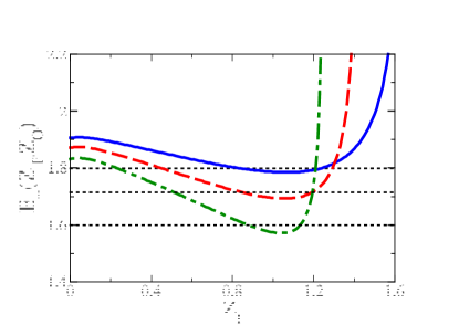
Figure 1: Energy functional $E_{\epsilon=-1}(Z_{I},Z_{O})$ in units of $\Delta$ for the spin singlet state as a function of $Z_{I}$ for $Z=1$, taking $Z_{O}=0.3$. The green dash-dotted (red dashed, blue solid) curve is for $\alpha=0.3\leavevmode\nobreak\ (0.35,\leavevmode\nobreak\ 0.4)$, respectively. Horizontal lines indicate the respective threshold energies $\Delta(1+2\gamma)$. When a minimum exists below the threshold (as is the case for all shown $\alpha$), a bound state is present.

Figure 1 shows that the energy functional for the singlet state with $Z=1$ has a minimum for all studied values of $\alpha$. Moreover, the energy minimum is located below the threshold, i.e., the binding energy is positive, and we have a two-body bound state in the spin singlet sector. In contrast to that, our variational approach predicts that the energy functional has a minimum also for the spin triplet sector, but the minimum is now above the threshold and thus does not describe a bound state. We also notice that the energy functional for $Z_{I}=Z_{O}=Z$ simply yields the ground-state energy of a two-particle state with the Coulomb repulsion treated within first-order perturbation theory. As anticipated above, we find $E_{-}(1,1)>\Delta(1+2\gamma)$, and therefore perturbation theory is not able to correctly describe the bound state for $Z=1$.

$\alpha$	$\bar{E}_{\rm-,b}$	$Z_{O}$	$Z_{I}$
$0.01$	$0.307$	$0.289$	$1.090$
$0.05$	$0.308$	$0.290$	$1.090$
$0.10$	$0.310$	$0.292$	$1.088$
$0.15$	$0.314$	$0.295$	$1.086$
$0.20$	$0.320$	$0.299$	$1.081$
$0.25$	$0.327$	$0.305$	$1.076$
$0.30$	$0.337$	$0.314$	$1.068$
$0.35$	$0.350$	$0.325$	$1.058$
$0.40$	$0.366$	$0.341$	$1.045$

Table 1: Rescaled binding energy $\bar{E}_{\rm-,b}$, see Eq. (32), for the two-body bound state in the spin singlet sector with $Z=1$ and several values of $\alpha$. These values are plotted in Fig. 2. We also specify the effective charges $Z_{O}$ and $Z_{I}$ minimizing the energy functional, cf. Fig. 3.

Table 1 lists the binding energy in the spin singlet sector for several values of $\alpha$. Note that both $Z_{I}$ and $Z_{O}$ are (well) below the critical value $Z_{\rm crit}=1/(2\alpha)$ for all cases considered in Table 1. The fact that for $Z=1$ the minimum happens to be at $Z_{O}<1$ and $Z_{I}>1$ (or vice versa, due to the symmetry of $E_{\epsilon}$) is rationalized by noting that only in this case the two factors $(Z_{I}-1){\cal V}_{I}$ and $(Z_{O}-1){\cal V}_{O}$ in Eq. (31) will have opposite sign. Physically, one quasiparticle then partially screens the impurity charge seen by the other quasiparticle.

We observe from Table 1 that relativistic effects tend to increase the binding energy. Approximately, we find the scaling $\bar{E}_{\rm-,b}-\bar{E}_{\rm-,b}^{(0)}\sim\alpha^{2}$ illustrated in Fig. 2. It is interesting to note that the variational parameter $Z_{O}$ increases with $\alpha$ while $Z_{I}$ decreases, see Fig. 3. Since the atomic Bohr radius is $\sim 1/Z\alpha$, we conclude that in the relativistic case the outer (inner) electron will be closer to (further away from) the nucleus than in the nonrelativistic case.

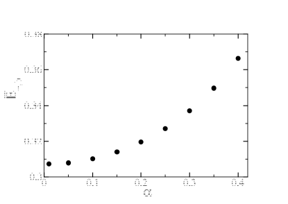
Figure 2: Rescaled dimensionless binding energy $\bar{E}_{\rm-,b}$ vs $\alpha$, see Eq. (32), in the spin singlet sector with $Z=1$.

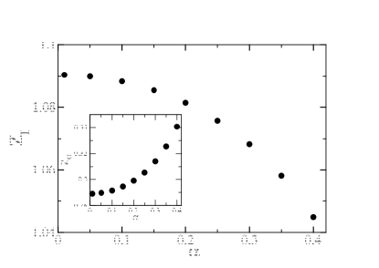
Figure 3: Optimal values of $Z_{I}$ (main panel) and $Z_{O}$ (inset) vs $\alpha$ for the spin singlet case with $Z=1$.

III.3 Validity of the variational approach

Before we conclude this section, we comment on the validity of this variational calculation. First, we observe that the single-particle orbital $|\Psi_{\lambda}\rangle$ is the normalized ground state of a modified Dirac Hamiltonian $H_{\lambda}$ which is related to $H_{\rm D}$ by

$$H_{\rm D}=H_{\lambda}+\frac{(Z_{\lambda}-Z)\alpha}{r}.$$ (33)

Assuming that $|\Psi_{E,j}\rangle$ is in the continuous spectrum of $H_{\rm D}$, we have

$$(E-E_{\lambda})\langle\Psi_{\lambda}|\Psi_{E,j}\rangle=\langle\Psi_{\lambda}|[(Z_{\lambda}-Z)\alpha/r]|\Psi_{E,j}\rangle.$$ (34)

As a consequence, for $E_{\lambda}\neq E$ and $Z_{\lambda}=Z$, the state $|\Psi_{\lambda}\rangle$ is orthogonal to $|\Psi_{E}\rangle$. This is to be expected since in that case, they are eigenstates of the same Hermitian operator with different eigenvalues. However, for $Z_{\lambda}\neq Z$, both states will generically have a finite overlap. Since we take $|\Psi_{\lambda}\rangle$ as the ground-state orbital, it is clear that the overlap with states in the negative-energy continuum will be suppressed by a factor $\approx 1/\Delta$. Actually, the overlap $\langle\Psi_{\lambda}|\Psi_{E,j}\rangle$ can be evaluated analytically, see App. A. We can thereby compute the total weight of our variational wave function on the negative energy states,

$$W_{\lambda}(\alpha)=\int_{E<-\Delta}\frac{dE}{2\pi\sqrt{E^{2}-\Delta^{2}}}\left|\langle\Psi_{\lambda}|\Psi_{E,j}\rangle\right|^{2}.$$ (35)

The result is shown in Fig. 4 for several values of $\alpha$ and the corresponding $Z_{\lambda}$ from Table 1. We find that the total weight $W_{\lambda}(\alpha)$ for $\alpha\leq 0.4$ is at most of order $0.01$. It then stands to reason that neglecting the projection operator in the evaluation of Coulomb matrix elements does not significantly affect the variational estimate of the binding energy for $\alpha\lesssim 0.4$.

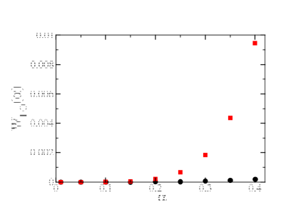
Figure 4: Cumulative weight $W_{\lambda}$ vs $\alpha$, see Eq. (35), of the negative energy states in the variational wave function for $Z=1$, where $\lambda=I$ ($\lambda=O$) corresponds to black circles (red squares).

IV Generalizations

So far we have restricted ourselves to the case of two quasiparticles in the same valley, in the presence of a band gap, and for an impurity of charge $Z=1$. In this section, we briefly address various extensions, namely (i) the case of an impurity with charge $Z>1$, (ii) a topological band gap, and (iii) quasiparticles in different valleys.

IV.1 Impurity charge $Z>1$

From a theoretical perspective, the case $Z>1$ is less interesting than $Z=1$ because a bound state is then found already in perturbation theory. In fact, when treating the two-body Coulomb interaction perturbatively, the energy of the lowest singlet state, taken in the simple factorized form $\Phi_{\rm tot}=\Psi_{0,\frac{1}{2}}({\bf r}_{1})\Psi_{0,\frac{1}{2}}({\bf r}_{2})|\chi\rangle$, coincides with the value of the energy functional $E_{\epsilon}(Z_{I},Z_{O})$ for $\epsilon=0$ and $Z_{I}=Z_{O}=Z$,

$$E_{\rm pert}=E_{0}(Z,Z)=4\Delta\gamma+{\cal V}_{\rm 2b}^{\rm dir}.$$ (36)

Straightforward evaluation of Eq. (36) then shows that the perturbative estimate for the binding energy $\bar{E}_{\rm-,b}$, cf. Eq. (32), is negative for $Z=1$ but positive for $Z>1$. Hence a bound state is predicted already by perturbation theory for $Z>1$, in contrast to the case $Z=1$.

Moreover, for $Z>1$, our variational method turns out to be restricted to rather small values of $\alpha$. Table 2 summarizes the rescaled binding energies, $\bar{E}_{\rm-,b}$, and the optimal charges, $Z_{I,O}$, for $Z=2$ and several values of $\alpha$. We here consider only the regime $\alpha\leq 0.2$ to ensure that the optimal charges remain well below the singular value $Z_{\rm crit}=1/(2\alpha)$.

For $Z>1$, we also find a bound state in the spin-triplet channel. However, the variational wave function used here for the triplet state is probably not the most appropriate. In the case of the helium atom, textbooks bransden show that the simplest wave function for the lowest triplet state combines the single-particle ground state and the first excited state. By analogy, for our 2D case, a better choice for the triplet case might be to take instead of Eq. (15) the ansatz

$$\Phi_{j=0}=\Psi_{0,\frac{1}{2},I}({\bf r}_{1})\Psi_{1,-\frac{1}{2},O}({\bf r}_{2})-\Psi_{1,-\frac{1}{2},O}({\bf r}_{1})\Psi_{0,\frac{1}{2},I}({\bf r}_{2}),$$ (37)

which is an eigenstate of the total angular momentum operator $J_{z}=J_{z}(1)+J_{z}(2)$ with eigenvalue $j=0$. Another option is

$$\Phi_{j=1}=\Psi_{0,\frac{1}{2},I}({\bf r}_{1})\Psi_{1,\frac{1}{2},O}({\bf r}_{2})-\Psi_{1,\frac{1}{2},O}({\bf r}_{1})\Psi_{0,\frac{1}{2},I}({\bf r}_{2}).$$ (38)

In the absence of Coulomb interactions, this state has the same energy as $\Phi_{j=0}$ but Coulomb interactions will mix them. Therefore a variational approach should take into account both of them. However, this analysis goes beyond the scope of this paper.

$\alpha$	$\bar{E}_{\rm-,b}$	$Z_{O}$	$Z_{I}$
$0.01$	$7.524$	$1.142$	$2.266$
$0.05$	$7.591$	$1.148$	$2.261$
$0.10$	$7.817$	$1.169$	$2.243$
$0.15$	$8.265$	$1.210$	$2.207$
$0.20$	$9.136$	$1.292$	$2.141$

Table 2: Rescaled binding energy $\bar{E}_{\rm-,b}$, see Eq. (32), for the two-particle bound state in the spin singlet sector for $Z=2$ and several values of $\alpha$. We also specify the effective charges $Z_{O}$ and $Z_{I}$ minimizing the energy functional.

IV.2 Topological band gap

Let us next consider the case of a topological gap, $H_{\rm so}=\Delta\sigma_{z}s_{z}$, see Eq. (8), where we set $\tau_{z}=1$ as we shall still assume that both quasiparticles are in the same valley. (For related studies of the case without Coulomb impurity, see Refs. rodin ; zhong ; trushin .) Since the total Hamiltonian now does not commute with ${\bf S}^{2}$ anymore, we must distinguish whether the two quasiparticles have same or opposite spin projections, $S_{z}=\pm 1$ or $S_{z}=0$. If both quasiparticles have the same spin projection (e.g., $S_{z}=1$), we are back to the case discussed in Sec. III but with $\epsilon=+1$ (spin triplet). Within our variational approach for $Z=1$, there is no stable bound state.

Turning now to $S_{z}=0$, we cannot separately consider spin singlet and triplet states. A natural way to construct the Chandrasekhar-Dirac variational wave function is as follows. We consider the 2D subspace spanned by the wave functions

$$\Phi_{1} = \Psi_{I,\uparrow}({\bf r}_{1})|\uparrow\rangle_{1}\otimes\Psi_{O,\downarrow}({\bf r}_{2})|\downarrow\rangle_{2}$$ (39)

$$-\Psi_{O,\downarrow}({\bf r}_{1})|\downarrow\rangle_{1}\otimes\Psi_{I,\uparrow}({\bf r}_{2})|\uparrow\rangle_{2},$$

$$\Phi_{2} = \Psi_{I,\downarrow}({\bf r}_{1})|\downarrow\rangle_{1}\otimes\Psi_{O,\uparrow}({\bf r}_{2})|\uparrow\rangle_{2}$$

$$-\Psi_{O,\uparrow}({\bf r}_{1})|\uparrow\rangle_{1}\otimes\Psi_{I,\downarrow}({\bf r}_{2})|\downarrow\rangle_{2},$$

where spin and orbital degrees of freedom are entangled. In Eq. (39), $|s\rangle_{l}$ is the eigenstate of $s_{z}$ with eigenvalue $s=\pm=\uparrow/\downarrow$ for particle $l=1,2$, and $\Psi_{\lambda,s}$ refers to the normalized ground state of the single-particle Hamiltonian

$$H_{\lambda,s}=-i{\bm{\sigma}}\cdot\nabla+s\Delta\sigma_{z}-\frac{Z_{\lambda}\alpha}{r},$$ (40)

with $\lambda=I,O$. Again, $Z_{I,O}$ are variational parameters, and the valley part is kept implicit. Since the valley part is assumed symmetric, we have to choose antisymmetric combinations in Eq. (39).

With the ground state of $H_{\lambda,+}$ given by

$$\Psi_{\lambda,\uparrow}\sim r^{\gamma_{\lambda}-1/2}e^{-p_{\lambda}r}\left(\begin{array}[]{c}1\\ i\kappa_{\lambda}e^{i\theta}\end{array}\right),$$ (41)

we directly obtain

$$\Psi_{\lambda,\downarrow}=-i\sigma_{y}(\Psi_{\lambda,\uparrow})^{*}\sim r^{\gamma_{\lambda}-1/2}e^{-p_{\lambda}r}\left(\begin{array}[]{c}i\kappa_{\lambda}e^{-i\theta}\\ 1\end{array}\right)$$ (42)

as ground state of $H_{\lambda,-}$ with the same energy, where $\langle\Psi_{I,\uparrow}|\Psi_{O,\downarrow}\rangle=0$. In the subspace spanned by the states $\Phi_{1,2}$, the Hamiltonian eigenvalue problem thus reduces to the problem of finding solutions of the secular equation

$$\det\left(\begin{array}[]{cc}H_{11}-2E&H_{12}-\Sigma_{12}E\\ H_{21}-\Sigma_{21}E&H_{22}-2E\end{array}\right)=0,$$ (43)

where we use the notation (with $a,b=1,2$)

$$H_{ab}=\langle\Phi_{a}|H|\Phi_{b}\rangle,\qquad\Sigma_{ab}=\langle\Phi_{a}|\Phi_{b}\rangle.$$ (44)

Using the results of Sec. III and noting that the single-particle matrix elements are independent of the spin projection, we find $\Sigma_{11}=\Sigma_{22}=2$ and $\Sigma_{12}=\Sigma_{21}=-2S^{2}$. The roots of the secular equation are given by

$$E_{\pm}(Z_{I},Z_{O})=\frac{2H_{11}-H_{12}\Sigma_{12}\pm\left|2H_{12}-H_{11}\Sigma_{12}\right|}{4-\Sigma_{12}^{2}},$$ (45)

It turns out that this expression has the same structure as the energy functional in Eq. (31), and the corresponding results therefore apply again. We conclude that the topological band gap caused by Eq. (8) does not imply different bound-state energies as compared to the topologically trivial band gap resulting from Eq. (7).

IV.3 Different valleys

So far we have assumed that the two quasiparticles occupy the same valley state, and we thus only have a trivial double degeneracy of the bound state. We shall now briefly discuss the case in which the two quasiparticles live in different valleys (cf. Ref. entin for a setting without Coulomb impurity). To properly address this situation, we first recall that the Dirac-Weyl spinors represent the slowly varying parts of the electronic wave function. The complete wave function is obtained by multiplying these spinors by the appropriate Bloch wave at the $K$ or $K^{\prime}$ point. In the continuum description, one neglects the overlap between wave functions in opposite valleys, $\langle K|K^{\prime}\rangle=0$. (Going beyond this approximation would require a study of the lattice model.) Second, we observe that $H_{0}$ in Eq. (5) does not commute with the total squared valley operator ${\bf T}^{2}$, where ${\bf T}={\bm{\tau}}_{1}+{\bm{\tau}}_{2}$. This fact must be taken into account when building the appropriate Chandrasekhar-Dirac wave function. Finally, the two-body Coulomb interaction potential has the same form as for two quasiparticles with the same valley quantum number, see App. B. A straightforward calculation as in Sec. IV.2 then shows that the resulting energy functional has the same structure as before. Therefore the optimal binding energy coincides with the one for both quasiparticles in the same valley.

V Observables

In this section, we turn to a discussion of the probability density and of the pair distribution function for the bound state. We consider the most interesting case $Z=1$ and focus on the Dirac band gap term in Eq. (7) for the two-body spin singlet state. However, using the results in Sec. IV, it is straightforward to obtain corresponding results also for other cases of interest.

V.1 Probability density

We start by calculating the probability density for the two-particle bound state. The density operator is $\hat{\rho}({\bf r})=\sum_{l=1,2}\delta({\bf r}-{\bf r}_{l}),$ and thus the probability density is given by

$$\rho({\bf r}) = \frac{1}{\langle\Phi|\Phi\rangle}\int d{\bf r}_{1}d{\bf r}_{2}\Phi^{\dagger}({\bf r}_{1},{\bf r}_{2})\,\hat{\rho}({\bf r})\,\Phi({\bf r}_{1},{\bf r}_{2})$$ (46)

$$= \int d{\bf r}_{2}\frac{\left|\Phi({\bf r},{\bf r}_{2})\right|^{2}}{1+S^{2}}.$$

The integral can be evaluated exactly, where the result for $\rho({\bf r})$ does not depend on the polar angle $\theta$. It is then convenient to consider the radial density,

$$P(r) = r\int d\theta\rho({\bf r})=\frac{1}{1+S^{2}}\Bigl{[}\sum_{\lambda}\frac{(2p_{\lambda})^{2\gamma_{\lambda}+1}}{\Gamma(2\gamma_{\lambda}+1)}r^{2\gamma_{\lambda}}e^{-2p_{\lambda}r}$$ (47)

$$+ 2S^{2}\frac{(p_{I}+p_{O})^{\gamma_{I}+\gamma_{O}+1}}{\Gamma(\gamma_{I}+\gamma_{O}+1)}r^{\gamma_{I}+\gamma_{O}}e^{-(p_{I}+p_{O})r}\Bigr{]},$$

with normalization $\int_{0}^{\infty}drP(r)=2$. The result is illustrated for $Z=1$ and several values of $\alpha$ in Fig. 5. With respect to the nonrelativistic case, we observe that relativistic effects tend to enhance the probability at small distance from the Coulomb impurity. Since the radial density can be probed by STM techniques, the result can be matched to the analytical result in Eq. (47). Thereby one can hope to extract, e.g., the value of the fine structure constant $\alpha$.

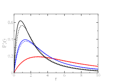
Figure 5: Radial density $P(r)$ vs distance $r$ from the impurity (in units of $\hbar v_{F}/\Delta$) of the spin-singlet two-body bound state, cf. Eq. (47), for $Z=1$ and several values of $\alpha$. Solid lines correspond to the relativistic case for $\alpha=0.1,\leavevmode\nobreak\ 0.2,$ and $0.3$, shown in red, blue, and black color (from bottom to top), respectively. Dashed lines indicate the corresponding nonrelativistic results.

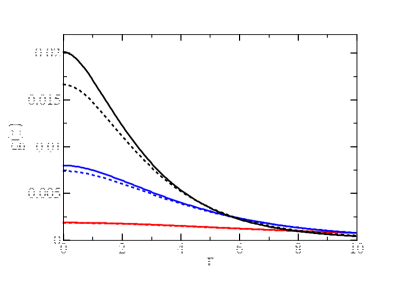
Figure 6: Radial profile of the pair distribution function, $g(r)$, vs interparticle distance $r$ (in units of $\hbar v_{F}/\Delta$) for $Z=1$ and several values of $\alpha$. Solid lines correspond to the relativistic case for $\alpha=0.1,\leavevmode\nobreak\ 0.2,$ and $0.3$, shown in red, blue, and black color (from bottom to top), respectively. Dashed lines indicate the corresponding nonrelativistic results.

V.2 Pair distribution function

Next we turn to the pair distribution function of the two-particle bound state,

$$g({\bf r}) = \frac{1}{2}\left\langle\sum_{i\neq j}\delta({\bf r}-({\bf r}_{i}-{\bf r}_{j})\right\rangle$$ (48)

$$= \int d{\bf r}_{1}\frac{|\Phi({\bf r}_{1}-{\bf r}/2,{\bf r}_{1}+{\bf r}/2)|^{2}}{\langle\Phi|\Phi\rangle}.$$

The result again turns out to be independent of the polar angle, $g=g(r)$, and is illustrated in Fig. 6. The pair distribution function can be experimentally obtained by a statistical analysis of STM images, see, e.g., Ref. Ertl , and can provide additional information about the existence and the properties of the two-body bound state predicted here.

VI Concluding remarks

In this work, we have studied the two-particle bound state problem for gapped graphene in the presence of a Coulomb impurity. We have shown that a variational approach, using the projected Hamiltonian and Chandrasekhar-Dirac spinors as trial wave functions, predicts the existence of at least one bound state. We found that in contrast to the Schrödinger case, the variational energy functional is not a homogeneous function of the coupling constant $\alpha$. As a consequence, the optimal values of the variational parameters $Z_{\lambda}$ depend on $\alpha$, and the optimal binding energy has a more complicated functional dependence on $\alpha$. In particular, the binding energy increases with respect to the nonrelativistic case. Moreover, we have determined the relativistic corrections to the probability density and to the pair probability density. The predicted two-body bound state can thereby be accessed experimentally, e.g., by means of STM techniques.

Finally, as a possibility for future theoretical work, it would be interesting to diagonalize the projected many-body Hamiltonian for graphene in a large basis set in order to compute the ground state energy without recourse to variational wave functions. This route can also provide information about low-lying excited resonant levels, which in turn are expected to exhibit Fano lineshapes when probed in transport or by STM methods.

Appendix A Relativistic 2D hydrogen atom

In order to keep the paper self-contained, we here collect known results for the single-particle Dirac-Coulomb problem in graphene, see, e.g., Refs. rmp1 ; kotov ; novikov ; gamayun . The massive Dirac-Weyl Hamiltonian with a Coulomb impurity of charge $Ze$ reads ($\hbar=v_{F}=1$)

$$H_{\rm D}=-i{\bm{\sigma}}\cdot\nabla+\Delta\sigma_{z}-\frac{Z\alpha}{r}.$$ (49)

The Hamiltonian (49) is exactly solvable, and the bound-state orbitals can be found, e.g., in Refs. novikov ; gamayun . Following the notation of Ref. novikov , in polar coordinates ($r,\theta$) they are given by

$$\Psi_{n,j}(r,\theta)={\cal N}_{n,j}\rho^{\gamma-\frac{1}{2}}e^{-\frac{\rho}{2}}\left(\begin{array}[]{r}(\varphi_{1}+c\varphi_{2})e^{i(j-\frac{1}{2})\theta}\\ i\kappa(\varphi_{1}-c\varphi_{2})e^{i(j+\frac{1}{2})\theta}\end{array}\right).$$ (50)

The half-integer index $j$ denotes the eigenvalue of the total angular momentum operator $J_{z}=-i\partial_{\theta}+\sigma_{z}/2$. The integer index $n\geq 0$ is the principal quantum number, where the energy eigenvalues are given by

$$E_{n,j}=\frac{\Delta}{\sqrt{1+\frac{Z^{2}\alpha^{2}}{(n+\gamma)^{2}}}}.$$ (51)

We use the notation

$$\rho = 2pr,\qquad p=\sqrt{\Delta^{2}-E^{2}},$$ (52)

$$\gamma = \sqrt{j^{2}-Z^{2}\alpha^{2}},\quad\kappa=\sqrt{\frac{\Delta-E}{\Delta+E}},$$

$$c = \frac{\gamma-\frac{Z\alpha E}{p}}{j+\frac{Z\alpha\Delta}{p}}=\frac{j-\frac{Z\alpha\Delta}{p}}{\gamma+\frac{Z\alpha E}{p}}.$$

The functions $\varphi_{1,2}$ in Eq. (50) are confluent hypergeometric functions of the first kind olver ,

$$\varphi_{1}(\rho) = M(\gamma-Z\alpha E/p,2\gamma+1,\rho),$$ (53)

$$\varphi_{2}(\rho) = M(\gamma+1-Z\alpha E/p,2\gamma+1,\rho).$$

Finally, ${\cal N}_{n,j}$ is a normalization constant such that $\int rdrd\theta|\Psi_{n,j}|^{2}=1$. Explicitly, one finds

$${\cal N}_{n,j}=\frac{(-1)^{n}p^{\frac{3}{2}}}{\Delta\Gamma(2\gamma+1)}\sqrt{\frac{\Gamma(2\gamma+1+n)(\Delta+E)(j+\frac{Z\alpha\Delta}{p})}{2\pi Z\alpha\,n!}}.$$ (54)

The energy eigenvalues (51) now follow from the condition $\gamma-Z\alpha E/p=-n$, such that the wave functions are normalizable. The confluent hypergeometric functions then reduce to generalized Laguerre polynomials olver ,

$$M(-n,2\gamma+1,\rho)=\frac{\Gamma(n+1)\Gamma(2\gamma+1)}{\Gamma(2\gamma+1+n)}L^{2\gamma}_{n}(\rho).$$ (55)

The $n>0$ bound states are doubly degenerate, $E_{n,j}=E_{n,-j}$, while the $n=0$ bound states exist only for $j>0$. Technically, this is due to the fact that for $n=0$, i.e., $\gamma-Z\alpha E/p=0$, $\varphi_{2}$ grows exponentially $\sim e^{\rho}$, and the corresponding solution is admissible only for $c=0$. This in turn occurs only for $j>0$, while $c=-1$ for $j<0$.

The lowest-energy bound state is given by

$$\Psi_{0,\frac{1}{2}}={\cal N}_{0,\frac{1}{2}}\rho^{\gamma-\frac{1}{2}}e^{-\frac{\rho}{2}}\left(\begin{array}[]{l}1\\ i\kappa e^{i\theta}\end{array}\right),$$ (56)

with the energy

$$E_{0,\frac{1}{2}}=2\Delta\gamma=\Delta\sqrt{1-4Z^{2}\alpha^{2}},$$ (57)

and the normalization factor

$${\cal N}_{0,\frac{1}{2}}=2Z\alpha\Delta\sqrt{\frac{2\gamma+1}{\pi\Gamma(2\gamma+1)}}.$$ (58)

States in the continuum spectrum, $|E|>\Delta$, can be obtained by means of analytic continuation in $E$, see Ref. novikov . One finds that the states are given by Eq. (50) with the substitutions

$$p = \sqrt{\Delta^{2}-E^{2}}\rightarrow-i\sqrt{E^{2}-\Delta^{2}}\equiv-i\tilde{p},$$ (59)

$$\rho = 2pr\rightarrow-2i\tilde{p}r,$$

$$c = \frac{\gamma-Z\alpha E/p}{j+Z\alpha\Delta/p}\to\frac{\gamma-iZ\alpha E/\tilde{p}}{j+iZ\alpha\Delta/\tilde{p}}\equiv e^{-2i\xi}\equiv\tilde{c}$$

$$\kappa = \sqrt{\frac{\Delta-E}{\Delta+E}}\rightarrow-i\,\text{sgn}(E)\,\sqrt{\frac{E-\Delta}{E+\Delta}}$$

$$\equiv -i\,\tilde{\kappa}=-i\frac{\tilde{p}}{E+\Delta}=-i\frac{E-\Delta}{\tilde{p}}.$$

Explicitly, we get

$$\Psi_{E,j}={\cal N}_{E,j}r^{\gamma-1/2}e^{i\tilde{p}r}\left(\begin{array}[]{r}(\varphi_{1}+\tilde{c}\varphi_{2})e^{i(j-\frac{1}{2})\theta}\\ \tilde{\kappa}(\varphi_{1}-\tilde{c}\varphi_{2})e^{i(j+\frac{1}{2})\theta}\end{array}\right),$$ (60)

where

$$\varphi_{1} = M(\gamma-iZ\alpha E/\tilde{p},2\gamma+1,-2i\tilde{p}r),$$ (61)

$$\varphi_{2} = M(\gamma+1-iZ\alpha E/\tilde{p},2\gamma+1,-2i\tilde{p}r).$$

The normalization factor ${\cal N}_{E,j}$ follows by matching the asymptotic behavior of Eq. (60) to that of free spherical spinors novikov , and reads

$${\cal N}_{E,j}=\left(\frac{|E+\Delta|}{2|E|}\right)^{\frac{1}{2}}\frac{|\Gamma(1+\gamma+\frac{iZ\alpha E}{\tilde{p}})|}{\sqrt{2\pi}\Gamma(2\gamma+1)}e^{\frac{\pi Z\alpha E}{2\tilde{p}}}(2\tilde{p})^{\gamma}e^{i\xi}.$$ (62)

The spinors then satisfy the identity

$$\int d{\bf r}\,\Psi^{\dagger}_{E,j}({\bf r})\Psi_{E^{\prime},j^{\prime}}({\bf r})=2\pi\delta(\tilde{p}-\tilde{p}^{\prime})\Theta(EE^{\prime})\delta_{jj^{\prime}},$$ (63)

where $\Theta$ is the Heaviside step function. Therefore the resolution of the identity for the (projected) Coulomb-Dirac problem reads

$${\mathbb{1}} = \sum_{n,j}|\Psi_{n,j}\rangle\langle\Psi_{n,j}|+$$

$$+ \sum_{j}\int_{|E|>\Delta}\frac{dE}{2\pi\sqrt{E^{2}-\Delta^{2}}}|\Psi_{E,j}\rangle\langle\Psi_{E,j}|.$$

Finally, we provide the overlaps between our variational wave function $|\Psi_{\lambda}\rangle$ in Eq. (16) and the bound states as well as with continuum states. Using the identity

$$\int_{0}^{\infty}e^{-\lambda r}r^{\nu}M(a,c,kr)dr=\frac{\Gamma(\nu+1)}{\lambda^{\nu+1}}{}_{2}F_{1}(a,\nu+1,c,k/\lambda),$$ (65)

where ${}_{2}F_{1}(a,b,c,z)$ is the hypergeometric function olver , the overlap integrals with bound states are given by

$$C_{n,j} = \langle\Psi_{\lambda}|\Psi_{n,j}\rangle=2\pi\delta_{j,\frac{1}{2}}{\cal N}_{\lambda}{\cal N}_{n,j}\frac{\Gamma(\gamma_{\lambda}+\gamma+1)}{(p_{\lambda}+p)^{\gamma_{\lambda}+\gamma+1}}\Biggl{[}\left(1+\frac{2\alpha_{\lambda}(\Delta-E_{n,j})}{(2\gamma_{\lambda}+1)p}\right){}_{2}F_{1}\left(-n,\gamma_{\lambda}+\gamma+1,2\gamma+1,\frac{2p}{p_{\lambda}+p}\right)$$ (66)

$$- \frac{n}{j+\alpha\Delta/p}\left(1-\frac{2\alpha_{\lambda}(\Delta-E_{n,j})}{(2\gamma_{\lambda}+1)p}\right){}_{2}F_{1}\left(-n+1,\gamma_{\lambda}+\gamma+1,2\gamma+1,\frac{2p}{p_{\lambda}+p}\right)\Biggr{]},$$

while the overlap with continuum states is given by

$$C_{j}(E) = \langle\Psi_{\lambda}|\Psi_{E,j}\rangle=2\pi\delta_{j,\frac{1}{2}}{\cal N}_{\lambda}{\cal N}_{E,j}\int_{0}^{\infty}dr\,r^{\gamma_{\lambda}+\gamma}e^{-(2\alpha_{\lambda}-i\tilde{p})r}\left[(1-i\tilde{\kappa}\kappa_{\lambda})\varphi_{1}+c(1+i\tilde{\kappa}\kappa_{\lambda})\varphi_{2}\right],$$ (67)

$$= 2\pi\delta_{j,\frac{1}{2}}{\cal N}_{\lambda}{\cal N}_{E,\frac{1}{2}}\frac{\Gamma(\gamma_{\lambda}+\gamma+1)}{(p_{\lambda}-i\tilde{p})^{\gamma_{\lambda}+\gamma+1}}\Biggl{[}\left(1-i\frac{2\alpha_{\lambda}(E-\Delta)}{(2\gamma_{\lambda}+1)\tilde{p}}\right){}_{2}F_{1}\left(\gamma-i\alpha E/\tilde{p},\gamma_{\lambda}+\gamma+1,2\gamma+1,\frac{-2i\tilde{p}}{p_{\lambda}-i\tilde{p}}\right)$$

$$+ \frac{\gamma-i\alpha E/\tilde{p}}{j+i\Delta\alpha/\tilde{p}}\left(1+i\frac{2\alpha_{\lambda}(E-\Delta)}{(2\gamma_{\lambda}+1)\tilde{p}}\right){}_{2}F_{1}\left(\gamma-i\alpha E/\tilde{p}+1,\gamma_{\lambda}+\gamma+1,2\gamma+1,\frac{-2i\tilde{p}}{p_{\lambda}-i\tilde{p}}\right)\Biggr{]}.$$

Using the identity ${}_{2}F_{1}(a,b,b,z)=(1-z)^{-a}$, one can check that for $Z_{\lambda}=Z$, the overlaps $C_{n,j}$ reduce to $\delta_{n,0}\delta_{j,1/2}$ and that the overlaps $C_{j}(E)$ vanish. Furthermore, since the $|\Psi_{\lambda}\rangle$ states are normalized to unity, the expansion coefficients satisfy the identity

$$\sum_{n,j}|C_{n,j}|^{2}+\sum_{j}\int\frac{dE}{2\pi\sqrt{E^{2}-\Delta^{2}}}|C_{j}(E)|^{2}=1.$$ (68)

Appendix B Coulomb interaction

Here we briefly discuss the form of the two-body interaction used in our analysis. In general, the many-body Coulomb interaction is given by

$$H_{\rm int}=\frac{1}{2}\int d{\bf r}_{1}d{\bf r}_{2}\Psi_{s_{1}}^{\dagger}({\bf r}_{1})\Psi^{\dagger}_{s_{2}}({\bf r}_{2})V_{\rm 2b}({\bf r}_{12})\Psi_{s_{2}}({\bf r}_{2})\Psi_{s_{1}}({\bf r}_{1})$$ (69)

where $\Psi_{s}(\bf r)$ is the field operator with spin projection $s=\pm 1$, and the sum over spin projections is understood. For graphene, the field operator in the continuum limit can be decomposed into valley components,

$$\Psi_{s}({\bf r})\simeq\sum_{\tau=\pm}e^{i\tau{\bf K}\cdot{\bf r}}\Psi_{s,\tau}({\bf r}),$$

where $\pm{\bf K}$ are the two independent Fermi momenta (Dirac points) and $\tau=\pm$ is the valley index.

Correspondingly, $H_{\rm int}$ decomposes into several terms, $H_{\rm int}\simeq\sum_{j=1}^{5}H^{(j)}_{\rm int}$, where (the sum over repeated spin and valley indices is understood, and $\bar{\tau}=-\tau$)

$$H^{(1)}_{\rm int} = \frac{1}{2}\int d{\bf r}_{1}d{\bf r}_{2}\;\Psi_{s_{1},\tau}^{\dagger}({\bf r}_{1})\Psi^{\dagger}_{s_{2},\tau}({\bf r}_{2})V_{\rm 2b}({\bf r}_{12})\Psi_{s_{2},\tau}({\bf r}_{2})\Psi_{s_{1},\tau}({\bf r}_{1}),$$

$$H^{(2)}_{\rm int} = \frac{1}{2}\int d{\bf r}_{1}d{\bf r}_{2}\;\Psi_{s_{1},\tau}^{\dagger}({\bf r}_{1})\Psi^{\dagger}_{s_{2},\bar{\tau}}({\bf r}_{2})V_{\rm 2b}({\bf r}_{12})\Psi_{s_{2},\bar{\tau}}({\bf r}_{2})\Psi_{s_{1},\tau}({\bf r}_{1}),$$

$$H^{(3)}_{\rm int} = \frac{\tilde{V}_{\rm 2b}(2{\bf K})}{2}\int d{\bf R}\;\Psi_{s_{1},\tau}^{\dagger}({\bf R})\Psi^{\dagger}_{s_{2},\bar{\tau}}({\bf R})\Psi_{s_{2},\tau}({\bf R})\Psi_{s_{1},\bar{\tau}}({\bf R}),$$ (70)

$$H^{(4)}_{\rm int} = \frac{1}{2}\int d{\bf r}_{1}d{\bf r}_{2}\;\Psi_{s_{1},\tau}^{\dagger}({\bf r}_{1})\Psi^{\dagger}_{s_{2},\tau}({\bf r}_{2})e^{-i2\tau{\bf K}\cdot({\bf{\bf r}_{1}+{\bf r}_{2}})}V_{\rm 2b}({\bf r}_{12})\Psi_{s_{2},\bar{\tau}}({\bf r}_{2})\Psi_{s_{1},\bar{\tau}}({\bf r}_{1}),$$

$$H^{(5)}_{\rm int} = \frac{\tilde{V}_{\rm 2b}({\bf K})}{2}\int d{\bf R}\;\Psi_{s_{1},\tau_{1}}^{\dagger}({\bf R})\Psi^{\dagger}_{s_{2},\tau_{2}}({\bf R})e^{-i2\tau_{1}{\bf K}\cdot{\bf R}}\Psi_{s_{2},\tau_{2}}({\bf R})\Psi_{s_{1},\bar{\tau}_{1}}({\bf R})$$ (71)

$$+ \frac{\tilde{V}_{\rm 2b}({\bf K})}{2}\int d{\bf R}\;\Psi_{s_{1},\tau_{1}}^{\dagger}({\bf R})\Psi^{\dagger}_{s_{2},\tau_{2}}({\bf R})e^{-i2\tau_{2}{\bf K}\cdot{\bf R}}\Psi_{s_{2},\bar{\tau}_{2}}({\bf R})\Psi_{s_{1},\tau_{1}}({\bf R}).$$

In order to obtain Eqs. (70) and (71), we have switched to center-of-mass and relative coordinates, ${\bf R}=({\bf r}_{1}+{\bf r}_{2})/2$ and ${\bf r}={\bf r}_{1}-{\bf r}_{2}$, respectively, and subsequently integrated over the relative coordinate. Furthermore, $\tilde{V}_{\rm 2b}({\bf q})$ denotes the Fourier component of the Coulomb potential, where ${\bf q}={\bf K}$ or ${\bf q}=2{\bf K}$.

For our problem, we expect that the dominant matrix elements of $H_{\rm int}$ in the two-particle subspace are those due to $H^{(1)}_{\rm int}$ if both particles belong to the same valley, or those due to $H^{(2)}_{\rm int}$ if they belong to opposite valleys. The matrix elements of all other terms are suppressed either by a small coupling constant $[H^{(3)}_{\rm int}]$, due to rapidly fluctuating exponential factors in the integral $[H^{(4)}_{\rm int}]$, or by both mechanisms together $[H^{(5)}_{\rm int}]$.

References

• (1) K.S. Novoselov, A.K. Geim, S.V. Morozov, D. Jiang, Y. Zhang, S.V. Dubonos, I.V. Grigorieva, and A.A. Firsov, Science 306, 666 (2004).
• (2) K.S. Novoselov, A.K. Geim, S.V. Morozov, D.Jiang, M.I. Katsnelson, I.V. Grigorieva, S.V. Dubonos, and A.A. Firsov, Nature 438, 197 (2005).
• (3) A.H. Castro Neto, F. Guinea, N.M.R. Peres, K.S. Novoselov, and A. Geim, Rev. Mod. Phys. 81, 109 (2009).
• (4) M.O. Goerbig, Rev. Mod. Phys. 83, 1193 (2011).
• (5) A.F. Young and P. Kim, Annu. Rev. Condens. Matter Phys. 2, 101 (2011).
• (6) E.Y. Andrei, G. Li, and X. Du, Rep. Prog. Phys. 75, 056501 (2012).
• (7) V.N. Kotov, B. Uchoa, V.M. Pereira, A.H. Castro-Neto, and F. Guinea, Rev. Mod. Phys. 84, 1067 (2012).
• (8) V.A. Miransky and I.A. Shovkovy, Phys. Rep. 576, 1 (2015).
• (9) M. Kim, J.H. Choi, S.H. Lee, K. Watanabe, T. Taniguchi, S.H. Jhi, and H.J. Lee, Nat. Phys. 12, 1022 (2016).
• (10) C.R. Dean et al., Nature Nanotech. 5, 722 (2010).
• (11) M.A.H. Vozmediano, M.I. Katsnelson, and F. Guinea, Phys. Rep. 496, 109 (2010).
• (12) C.L. Kane and E.J. Mele, Phys. Rev. Lett. 95, 226801 (2005).
• (13) D. Huertas-Hernando, F. Guinea, and A. Brataas, Phys. Rev. B 74, 155426 (2006).
• (14) L.A. Ponomarenko et al., Nature 497, 594 (2013).
• (15) J.C.W. Song, A.V. Shytov, and L.S. Levitov, Phys. Rev. Lett. 111, 266801 (2013).
• (16) Y. Wang, V.W. Brar, A.V. Shytov, Q. Wu, W. Regan, H.Z. Tsai, A. Zettl, L.S. Levitov, and M.F. Crommie, Nat. Phys. 6, 653 (2012).
• (17) A. Luican-Mayer, M. Kharitonov, G. Li, C.P. Lu, I. Skachko, A.-M.B. Gonçalves, K. Watanabe, T. Taniguchi, and E.Y. Andrei, Phys. Rev. Lett. 112, 036804 (2014).
• (18) Y. Wang et al., Science 340, 734 (2013).
• (19) J. Lee et al., Nat. Phys. 12, 1032 (2016).
• (20) C. Gutiérrez, L. Brown, C.J. Kim, J. Park, and A.N. Pasupathy, Nat. Phys. 12, 1069 (2016).
• (21) D.S. Novikov, Phys. Rev. B 76, 245435 (2007).
• (22) O.V. Gamayun, E.V. Gorbar, and V.P. Gusynin, Phys. Rev. B 80, 165429 (2009).
• (23) J. Sabio, F. Sols, and F. Guinea, Phys. Rev. B 81, 045428 (2010).
• (24) R.N. Lee, A.I. Milstein, and I.S. Terekhov, Phys. Rev. B 86, 035425 (2012).
• (25) J.H. Grönqvist, T. Stroucken, M. Lindberg, and S.W. Koch, Eur. Phys. J. B 85, 395 (2012).
• (26) O.L. Berman, R. Ya. Kezerashvili, and K. Ziegler, Phys. Rev. A 87, 042513 (2013).
• (27) M.M. Mahmoodian and M.V. Entin, Europhys. Lett. 102, 37012 (2013).
• (28) C. Gaul, F. Domínguez-Adame, F. Sols, and I. Zapata, Phys. Rev. B 89, 045420 (2014).
• (29) L.L. Marnham and A.V. Shytov, Phys. Rev. B 92, 085409 (2015).
• (30) C.A. Downing and M.E. Portnoi, arXiv:1506.04425.
• (31) A.S. Rodin and A.H. Castro Neto, Phys. Rev. B 88, 195437 (2013).
• (32) J. Li, Y.L. Zhong, and D. Zhang, J. Phys. Cond. Matt. 27, 315301 (2015).
• (33) M. Trushin, M.O. Goerbig, and W. Belzig, Phys. Rev. B 94, 041301(R) (2016).
• (34) S. Chandrasekhar, Astrophys. J. 100, 176 (1944).
• (35) H.A. Bethe and E.E. Salpeter, Quantum Mechanics of One- and Two-Electron Atoms (Academic Press, New York, 1957).
• (36) R.N. Hill, J. Math. Phys. 18, 2316 (1977).
• (37) B.H. Bransden and C.J. Joachain, Physics of atoms and molecules (Longmont Group Limited, Hong Kong, 1983).
• (38) T. Andersen, Phys. Rep. 394, 157 (2004).
• (39) H. Hogaasen, J.-M. Richard, and P. Sorba, Am. J. Phys. 78, 86 (2010).
• (40) D.E. Phelps and K.K. Bajaj, Phys. Rev. B 27, 4883 (1983).
• (41) T. Pang and S.G. Louie, Phys. Rev. Lett. 65, 1635 (1990).
• (42) D.M. Larsen and S.Y. McCann, Phys. Rev. B 45, 3485 (1992).
• (43) D.M. Larsen and S.Y. McCann, Phys. Rev. B 46, 3966 (1992).
• (44) N.P. Sandler and C.R. Proetto, Phys. Rev. B 46, 7707 (1992).
• (45) M.V. Ivanov and P. Schmelcher, Phys. Rev. B 65, 205313 (2002).
• (46) S. Huant, S.P. Najda, and B. Etienne, Phys. Rev. Lett. 65, 1486 (1990).
• (47) A.J. Shields, M. Pepper, M.Y. Simmons, and D.A. Ritchie, Phys. Rev. B 52, 7841 (1995).
• (48) G.E. Brown and D.G. Ravenhall, Proc. Royal Soc. A 208, 552 (1951).
• (49) A. Kolakowska, J.D. Talman, and K. Aashamar, Phys. Rev. A 53, 168 (1996).
• (50) H. Nakatsuji and H. Nakashima, Phys. Rev. Lett. 95, 050407 (2005).
• (51) J. Sucher, Phys. Rev. A 22, 348 (1980).
• (52) J. Sucher, Int. J. Quantum Chem. 25, 3 (1984).
• (53) W. Häusler and R. Egger, Phys. Rev. B 80, 161402(R) (2009).
• (54) R. Egger, A. De Martino, H. Siedentop, and E. Stockmeyer, J. Phys. A 43, 215202 (2010).
• (55) F.W.J. Olver, D.W. Lozier, R.F. Boisvert, and C.W. Clark, NIST Handbook of Mathematical Functions (Cambridge University Press, NY, 2010).
• (56) J. Trost, T. Zambelli, J. Wintterlin, and G. Ertl, Phys. Rev. B 54, 17850 (1996).