Deep Variational Inference Without Pixel-Wise Reconstruction

Abstract

Variational autoencoders (VAEs), that are built upon deep neural networks have emerged as popular generative models in computer vision. Most of the work towards improving variational autoencoders has focused mainly on making the approximations to the posterior flexible and accurate, leading to tremendous progress. However, there have been limited efforts to replace pixel-wise reconstruction, which have known shortcomings. In this work, we use real-valued non-volume preserving transformations (real NVP) to exactly compute the conditional likelihood of the data given the latent distribution. We show that a simple VAE with this form of reconstruction is competitive with complicated VAE structures, on image modeling tasks. As part of our model, we develop powerful conditional coupling layers that enable real NVP to learn with fewer intermediate layers.

1 Introduction

In recent years, variational autoencoders (VAEs) [10, 19] have become extremely popular for many machine learning problems. They have been used for a variety of applications such as image modeling [4, 5], interpretable representation learning [12], conditional image generation [8, 15] and 3D structure learning from images [17]. VAEs provide a mathematically sound framework for unsupervised learning by optimizing the variational lower bound on the data likelihood. This lower bound involves two terms, (i) KL divergence of the approximate posterior with a fixed prior and (ii) conditional likelihood of the data given the latent distribution (also known as ‘reconstruction’). Much of the work in improving VAEs has focused on modifying the approximate posterior for better expressivity and approximations [2, 9, 18, 20]. On the other hand, little work has been done to improve upon the form of the reconstruction. Most VAE models assume a standard normal distribution for pixels in the reconstructed image space that leads to a mean-squared reconstruction cost. This has been previously shown to cause blurriness in the reconstructed images. Previous work has attempted to circumvent the problem by augmenting the model with generative adversarial networks [13, 16]. However, these models do not allow one to compute the conditional likelihood term exactly which limits our ability to objectively compare them with other VAE models. Other models have used alternatives like discrete softmax distribution [21] and discretized logistic distribution [9] for pixels, but these have not been well studied on their own.

Real-valued non-volume preserving transformations (real NVP) [3] offer exact likelihood computation through non-linear invertible transformations whose Jacobian determinants are easy to compute. This model also provides exact inversion from the latent space to the data space enabling efficient sampling, which is not available in other exact likelihood methods such as pixel recurrent neural networks (Pixel RNN) [21] and pixel convolutional neural networks (Pixel CNN) [22]. We use real NVP transformations to exactly compute the conditional likelihood term in a VAE and thus alleviate the problem of mean-squared reconstruction. We show that just using this modification we can compete with other complicated VAE models such as convolutional DRAW [4] (which uses multiple stochastic layers and recursion for sample generation) as well as real NVP [3] (using a smaller architecture). A summary of our contributions is as follows:

(1) We propose a model that uses real NVP transformations to model the conditional likelihood of the data given the latent distribution in a VAE.

(2) We propose a conditional coupling layer to make conditioning on the latent distribution stronger, adding multiplicative interactions to enable expressivity in the model with fewer layers.

(3) We compare the model against a complicated VAE model (convolutional DRAW) and also against other state-of-the-art generative models.

In the following section we review some of the preliminaries, and then go on to describe our model formally.

2 Background

2.1 Variational autoencoder

Variational autoencoders differ from regular autoencoders in that they have one or more stochastic layers for latent variables. These latent variables form the approximate posterior $q(z|x)$, which is forced to be close to a chosen prior such as a standard normal distrbution. This is achieved by minimizing the KL divergence between the approximate posterior and the prior, one of two terms in the variational lower bound for the log-likelihood of the data [10]:

$$\text{log}(p(x))\geq\mathbb{E}_{q(z|x)}[\text{log}(p(x|z))]-\text{KL}(q(z|x)||p(z))$$ (1)

Here, $q(z|x)$ is the approximate posterior modeled by the encoder, $p(x|z)$ is the conditional likelihood modeled by the decoder and $p(z)$ is the fixed prior distribution. In an unsupervised learning setup, one maximizes the variational lower bound as a surrogate for the log-likelihood. The expectation term is estimated using Monte Carlo sampling over the batch, $\mathbb{E}_{q(z|x)}[\text{log}(p(x|z))]\approx\frac{1}{n}\sum_{i=1}^{n}\text{log}(p(x_{i}|z_{i}))$, where $x_{i},i=1,2,\dots,n$ is a training example in the batch. In this work, we improve upon the technique to calculate $p(x_{i}|z_{i})$. Instead of assuming that the reconstructed image space follows a standard normal distribution, we assume that an intermediate layer follows a parametrized normal distribution. We provide more details in the next section.

2.2 Real NVP

Real NVP [3] is an exact likelihood model, that transforms the data into a prior probability distribution. Let us say that the data space $X$ is transformed into the space $Y$ through the function $f$. The change of variable formula for this transformation is given by the following equation:

$$p_{X}(x) =p_{Y}(f(x))\left|\text{det}\left(\frac{\partial f(x)}{\partial x^{T}}\right)\right|$$ (2)

Here, $x$ is a point in the data space. From the above equation, the likelihood of the data can be estimated if we can compute the two terms on the right. The likelihood of $f(x)$ in the space $Y$ can be computed analytically if we assume a prior such as a standard normal distribution in that space. To compute the second term, we need to be able to calculate the determinant of the Jacobian of the transformation $f(x)$. As we will see, this is enabled by the coupling layer transform. Also, if $f(x)$ is invertible, we can easily go from the latent space to the data space, $x=f^{-1}(y)$.

Let $x$ be the input to the coupling layer and $y$ be the expected output, each of the vectors are assumed to be $D$ dimensional. The coupling layer transform is given by [3]:

$$y_{1:d} =x_{1:d}$$ (3)

$$y_{d+1:D} =x_{d+1:D}\odot\text{exp}(l(x_{1:d}))+m(x_{1:d})$$ (4)

Here, $l$ and $m$ are arbitrary functions, which can be realized using neural networks. The transform divides the input vector into two parts, where the first part is kept unchanged and the second part is transformed using a function of the unchanged part.

The coupling layer transform can be inverted using the following equations:

$$x_{1:d} =y_{1:d}$$ (5)

$$x_{d+1:D} =(y_{d+1:D}-m(y_{1:d}))\odot\text{exp}(-l(y_{1:d}))$$ (6)

The computational complexity of computing the inverse is the same as going in the forward direction. If $f(x)$ is taken as a series of coupling layers, then one can compute $f^{-1}$ as each of the coupling layers is invertible.

The Jacobian of the coupling layer transform is as follows:

$$\frac{\partial y}{\partial x^{T}} =\begin{bmatrix}\mathbb{I}_{d}&0\\ \frac{\partial y_{d+1:D}}{\partial x_{1:d}^{T}}&\text{diag}(\text{exp}(l(x_{1:d})))\end{bmatrix}$$ (7)

Here, $\mathbb{I}_{d}$ is a $d$-dimensional identity matrix. The transformation gives a triangular Jacobian whose determinant is very easy to compute. From the above equation,

$$\text{det}\left(\frac{\partial y}{\partial x^{T}}\right)=\text{exp}\left(\sum l(x_{1:d})\right)$$ (8)

The summation is over the components of $l(x_{1:d})$. One can see the effect of a series of coupling layer transforms on the determinant of the Jacobian. If the data is transformed from $x$ to $y_{1}$, and from $y_{1}$ to $y_{2}$, one can compute the determinant as follows:

$$\text{det}\left(\frac{\partial y_{2}}{\partial x^{T}}\right) =\text{det}\left(\left(\frac{\partial y_{2}}{\partial y_{1}^{T}}\right)\left(\frac{\partial y_{1}}{\partial x^{T}}\right)\right)$$

$$=\text{det}\left(\frac{\partial y_{2}}{\partial y_{1}^{T}}\right)\text{det}\left(\frac{\partial y_{1}}{\partial x^{T}}\right)$$ (9)

This shows that one can compute the determinant of the Jacobian of $f(x)$ taken as a series of coupling layers by just multplying determinants of the Jacobians of the individual coupling layers. This enables us to compose $f(x)$ using an arbitrary number of coupling layers. Because of the above mentioned properties of the coupling layer transform, we can now compute the exact likelihood of the data. Thus, the network can be optimized using the maximum likelihood framework.

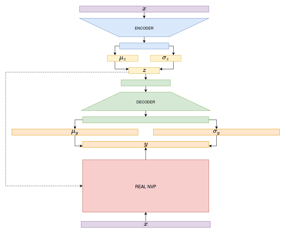
Figure 1: Block diagram of VAPNEV, color coded to indicate independent components. The dotted line suggests that the latent distribution may or may not be used for conditioning in the coupling layer transforms. The figure is illustrative of relative network sizes.

3 Our model: VAPNEV

In this section, we formally describe our model with the architectural novelties that we use. We call our model VAPNEV, which is an anagram for VAE-NVP.

3.1 Conditional likelihood calculation

In a regular VAE, the reconstructed image space is assumed to follow a normal distribution. Instead, here we assume an intermediate space $Y$ to follow a normal distribution. In order to calculate $p(x|z)$, we can transform the data space $X$ into the intermediate space $Y$ that depends on VAE latent space $Z$. The change of variable formula for this transformation is:

$$p(x|z) =p(f_{z}(x)|z)\left|\text{det}\left(\frac{\partial f_{z}(x)}{\partial x^{T}}\right)\right|$$ (10)

Here, $f_{z}(x)$ is a function that projects from the space $X$ to the space $Y$. In general, the transformation can depend on $z$ indicated by the subscript. If we assume $Y\sim\mathcal{N}(\mu_{y},\Sigma_{y})$, where $\mu_{y}=\phi_{1}(z)$ and $\Sigma_{y}=\text{diag}(\phi_{2}(z))$, log($p(f_{z}(x)|z)$) can be calculated using:

$$\text{log}(p(f_{z}(x)|z))= -\frac{1}{2}\text{log}(|\Sigma_{y}|)$$

$$-\frac{1}{2}(f_{z}(x)-\mu_{y})^{T}\Sigma_{y}^{-1}(f_{z}(x)-\mu_{y})$$

$$-\frac{D}{2}\text{log}(2\pi)$$ (11)

where $D$ is the dimensionality of the space. The determinant of the Jacobian $\left|\text{det}\left(\frac{\partial f_{z}(x)}{\partial x^{T}}\right)\right|$ can be computed if $f_{z}(x)$ is taken to be a series of coupling layers, as seen in the previous section. Thus, using this formulation with real NVP, one can completely avoid pixel-wise computation and still exactly calculate the conditional likelihood. It should be noted that the formulation holds even if $f_{z}(x)$ does not depend on $z$. As can be seen in Figure 1, VAPNEV models the prior space of the NVP using the decoder output.

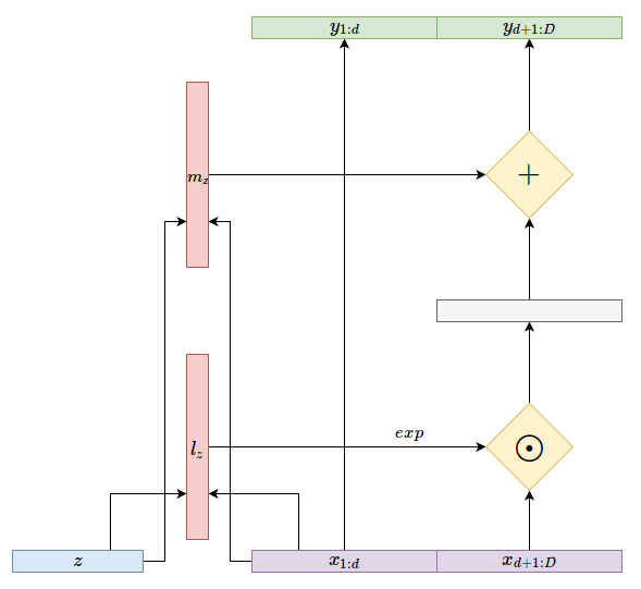
Figure 2: Conditional coupling layer

3.2 Conditional coupling layer

In order to make $f_{z}(x)$ conditional on the latent distribution of the VAE we propose the conditional coupling layer. This layer satisfies the following two conditions which are necessary for it to be useful in the above scenario, (i) the determinant of the Jacobian should be easy to compute and (ii) it should be invertible given $z$. The first condition ensures efficient computation of the cost of the model, whereas the second condition is essential for efficient sampling. The conditional coupling layer transform is very similar to the original transform and is given by:

$$y_{1:d} =x_{1:d}$$ (12)

$$y_{d+1:D} =x_{d+1:D}\odot\text{exp}(l_{z}(x_{1:d}))+m_{z}(x_{1:d})$$ (13)

Here, $x$ and $z$ are input to the layer, and $y$ is the output of the layer, $x$ and $y$ being $D$-dimensional. $l_{z}$ and $m_{z}$ can be arbitrary functions dependent on $z$. As for the regular coupling layers, this transformation gives us a diagonal Jacobian, whose determinant is easy to compute. The inverse can also be computed using very similar equations, provided $z$ is a known value:

$$x_{1:d} =y_{1:d}$$ (14)

$$x_{d+1:D} =(y_{d+1:D}-m_{z}(y_{1:d}))\odot\text{exp}(-l_{z}(y_{1:d}))$$ (15)

A graphical representation of the conditional coupling layer is shown in Figure 2. We now discuss the exact form of $l_{z}(x)$, which is also used for $m_{z}(x)$. From the transformation equations it is apparent that $l_{z}(x)$ should project to $\mathbb{R}^{D-d}$. To achieve this, we project each of $x$ and $z$ to $\mathbb{R}^{D-d}$ using functions $l_{1}$ and $l_{2}$ respectively, and then operate in an elementwise fashion on the computed function values. Note that here $x\in\mathbb{R}^{d}$ and if we take $d=D/2$, then $l_{1}$ can be a residual network [6] that maintains the dimensionality of $x$. Since $z$ is generally a low dimensional vector, we take $l_{2}$ to be a deconvolution network. Inspired by [23], we use multiplicative interactions between $l_{1}(x)$ and $l_{2}(z)$ to increase expressivity of the function. We summarize $l_{z}(x)$ using the following equation:

$$l_{z}(x) =\alpha\odot l_{1}(x)\odot l_{2}(z)+\beta_{1}\odot l_{1}(x)+\beta_{2}\odot l_{2}(z)+b$$ (16)

Since both $l_{1}(x)$ and $l_{2}(z)$ are outputs of convolutional networks, they are tensors in $\mathbb{R}^{H\text{x}W\text{x}C}$ ($H\text{x}W\text{x}C=D-d$). The multipliers $\alpha,\beta_{1},\beta_{2}$ and the bias $b$ are all in $\mathbb{R}^{C}$, and are trainable parameters. The elementwise multiplication with these multipliers uses broadcasting. The conditional coupling layer allows for shortcut connections to the VAE latent distribution which allows for stronger conditioning and faster training.

3.3 Training

The model is trained to maximixe the variational lower bound on the data log-likelihood. We summarize the feedforward computation of VAPNEV as shown in Figure 1:

$$\mu_{z} =\psi_{1}(x)$$ (17)

$$\sigma_{z} =\psi_{2}(x)$$ (18)

$$z\sim q(z|x) =\mathcal{N}(\mu_{z},\sigma_{z})$$ (19)

$$\mu_{y} =\phi_{1}(z)$$ (20)

$$\sigma_{y} =\phi_{2}(z)$$ (21)

$$y =f_{z}(x)$$ (22)

$\psi_{1}$ and $\psi_{2}$ include the encoder as well as the respective projections to the mean and variance of the approximate posterior. $z$ is sampled from the approximate posterior using the reparametrization trick [10]. $\phi_{1}$ and $\phi_{2}$ include the decoder as well as the respective projections to the mean and variance of the NVP latent space. $f_{z}(x)$ is the NVP network consisting of conditional coupling layers. Using $\mu_{z}$ and $\sigma_{z}$, the KL divergence term can be computed since we assume $p(z)=\mathcal{N}(0,I)$. $y$, $\mu_{y}$ and $\sigma_{y}$ are used to calculate $\text{log}(p(f_{z}(x)|z))$ and the adjustment $\text{log}\left(\left|\text{det}\left(\frac{\partial f_{z}(x)}{\partial x^{T}}\right)\right|\right)$ is provided by $f_{z}(x)$, which gives us $\text{log}(p(x|z))$.

We face the same problem as in [1], where the KL divergence term quickly goes to zero, leading to undesirable local optima. We use the annealing procedure suggested in [1] to alleviate the issue. We optimize our model using the ADAM optimizer [7] with default hyperparameters.

3.4 Generation

The generation process for VAPNEV is straightforward, which we summarize using the following equations:

$$z\sim p(z) =\mathcal{N}(0,I)$$ (23)

$$\mu_{y} =\phi_{1}(z)$$ (24)

$$\sigma_{y} =\phi_{2}(z)$$ (25)

$$y \sim\mathcal{N}(\mu_{y},\sigma_{y})$$ (26)

$$x =f_{z}^{-1}(y)$$ (27)

Unlike a regular VAE, a single $z$ might lead to different samples in VAPNEV, because of stochasticity in the $Y$ space. In case this is not desirable, we can pass $\mu_{y}$ into $f_{z}^{-1}$. We are able to calculate $f_{z}^{-1}(y)$ because of the invertibility property of the conditional coupling layer given $z$.

3.5 Reconstruction

Reconstruction of a given batch is very similar to the generative process, the only difference being that $z$ is sampled from the approximate posterior instead of the prior:

$$\mu_{z} =\psi_{1}(x)$$ (28)

$$\sigma_{z} =\psi_{2}(x)$$ (29)

$$z\sim q(z|x) =\mathcal{N}(\mu_{z},\sigma_{z})$$ (30)

$$\mu_{y} =\phi_{1}(z)$$ (31)

$$\sigma_{y} =\phi_{2}(z)$$ (32)

$$y \sim\mathcal{N}(\mu_{y},\sigma_{y})$$ (33)

$$x =f_{z}^{-1}(y)$$ (34)

The inverse of the NVP network can be seen as an extension of the decoder, as it is the final decoding step in the generation and reconstruction steps.

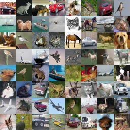
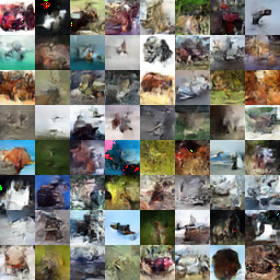
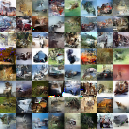
Figure 3: The left panel shows original images in the CIFAR-10 dataset. The middle panel shows the reconstructions of the images in the left panel. The right panel contains images sampled randomly from the model.

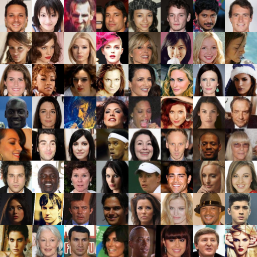
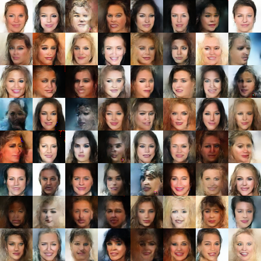
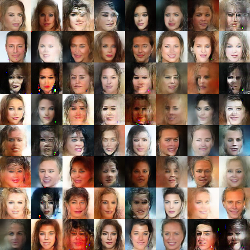
Figure 4: The left panel shows original images in the CelebA dataset. The middle panel shows the reconstructions of the images in the left panel. The right panel contains images sampled randomly from the model.

4 Experimental results

We test our model on the task of generative image modeling. The model is compared using natural images (CIFAR-10 [11]), as well as fixed domain images (CelebA [14]). First, we specify some common details used in all the experiments.

4.1 Modeling transformed data

The discrete image data in $[0,255]^{D}$ is first corrupted with uniform noise in $[0,1]$ to make it continuous, and is then scaled to $[0,1]^{D}$. Since real NVP gives a transformation from $\mathcal{R}^{D}$ to $\mathcal{R}^{D}$, we model the density of $\text{log}(\frac{x^{\prime}}{1-x^{\prime}})$ [3], which takes $x^{\prime}$ from $[0,1]^{D}$ to $\mathcal{R}^{D}$. Here, $x^{\prime}=\alpha+(1-\alpha)\odot x,\alpha\in[0,1]$, which is done to avoid numerical errors within the log. In our experiments, we take $\alpha=0.05$. To compute the actual variational lower bound, we have to account for this transformation. The correction factor comes out to be $\sum\text{log}\left(\frac{1-\alpha}{x^{\prime}\odot(1-x^{\prime})}\right)$, where the sum is over the components of $x^{\prime}$. We also use horizontal flips of the dataset images as data augmentation.

4.2 Architectural details

The encoder is taken as an 8-layer convolutional neural network. Every alternate layer doubles the number of filters and halves the spatial resolution in both directions. We start with 32 filters in the first layer. Analogous to the encoder, the decoder is an 8-layer deconvolution network, that doubles the spatial resolution and halves the number of filters every alternate layer. The first layer of this deconvolution network starts with the same dimensions as the output of the last encoder layer. The mean and variance of the VAE latent space are computed using separate fully-connected linear projections of the encoder output; the dimensionality of the latent space is taken to be 256. In case of the NVP latent space, the mean and variance are separate convolutional linear projections.

For the conditional coupling layer transform, we use checkerboard masking, channel-wise masking and the squeeze operation, all mentioned in [3]. To compute $l_{z}(x)$, we take $l_{1}(x)$ as a network of 2 residual blocks and $l_{2}(z)$ as a small deconvolution network. This deconvolution network starts with a tensor of $2\times 2\times c$, and doubles the spatial resolution at each layer. We take $c$ to be the number of filters in the residual blocks of the coupling layer. The same configuration is used for $m_{1}(x)$ and $m_{2}(z)$ in $m_{z}(x)$. We use a multi-scale architecture as mentioned in [3], with 2 scales. Each scale has 3 conditional coupling layers with checkerboard masking and 3 with channel-wise masking. We start with 64 filters for residual blocks in the first scale, and double them for the next scale. We use the same architecture for both the datasets.

Method	Bits/dim
PixelRNN [21]	3.00
IAF [9]	$<$ 3.28
Real NVP [3]	3.49
Conv DRAW [4]	$<$ 3.59
VAPNEV	$<$ 3.55

Table 1: Bits/dim on CIFAR-10. Lower is better.

4.3 CIFAR-10

From Table 1, we can see that VAPNEV is competitive with convolutional DRAW which is a complicated VAE structure with multiple stochastic layers and recurrent feedback. This establishes that replacing pixel-wise reconstruction with exact likelihood methods like real NVP is beneficial to the performance of VAEs. The model is also competitive with real NVP, which uses a much bigger architecture (8 residual blocks in coupling layers as opposed to 2 here). This shows the power of the conditional coupling layer transform, which is able to effectively utilize the semantic representation learned by the VAE latent distribution. As can be seen from the reconstructions in Figure 3, VAPNEV learns to model high level semantics in the latent distribution such as background color, pose and location of the object. The samples also show that the model is able to learn better global structure.

Method	Bits/dim
Real NVP [3]	3.02
VAPNEV	$<$ 2.8

Table 2: Bits/dim on CelebA. Lower is better.

4.4 CelebA

As shown in Table 2, VAPNEV performs significantly better than NVP on CelebA, while having a smaller architecture (The NVP model has 4 scales for CelebA, whereas VAPNEV uses 2). This suggests that NVP can be improved by using better global representations, learned here by the VAE. Looking at the reconstructions in Figure 4, we can see that the model learns high level semantic features such as hair color, face pose and expressions.

5 Discussion and future work

In this paper, we suggest a way to replace pixel-wise reconstruction with a maximum likelihood based alternative. We show that this greatly benefits the VAE formulation, as a simple VAE augmented with NVP transformations is able to compete with complicated models with multiple stochastic layers and recurrent connections. We develop powerful conditional coupling layer transforms which enable the model to learn with smaller architectures. VAPNEV provides a lot of advantages such as (i) it provides a way to replace pixel-wise reconstruction which has known shortcomings, (ii) it gives a generative model which can be trained and sampled from efficiently and (iii) it is a latent variable model which can be used for downstream supervised or semi-supervised learning.

This work can be extended in several ways. Using deeper architectures, and combining with expressive posterior computations like inverse autoregressive flow [9], it may be possible to compete with or even beat state-of-the-art models. This technique can be used to improve VAE models for other tasks such as semi-supervised learning and conditional density modeling. The conditional coupling layer can be used for constructing conditional real NVP models.

References

- [1] S. R. Bowman, L. Vilnis, O. Vinyals, A. M. Dai, R. Jozefowicz, and S. Bengio. Generating sentences from a continous space. CoNLL, 2016.
- [2] Y. Burda, R. Grosse, and R. Salakhutdinov. Importance weighted autoencoders. ICLR, 2016.
- [3] L. Dinh, J. Sohl-Dickstein, and S. Bengio. Density estimation using real nvp. arXiv preprint arXiv:1605.08803, 2016.
- [4] K. Gregor, F. Besse, D. J. Rezende, I. Danihelka, and D. Wierstra. Towards conceptual compression. NIPS, 2016.
- [5] K. Gregor, I. Danihelka, A. Graves, D. J. Rezende, and D. Wierstra. Draw: A recurrent neural network for image generation. ICML, 2015.
- [6] K. He, X. Zhang, S. Ren, and J. Sun. Deep residual learning for image recognition. CVPR, 2016.
- [7] D. P. Kingma and J. Ba. Adam: a method for stochastic optimization. ICLR, 2015.
- [8] D. P. Kingma, S. Mohamed, D. J. Rezende, and M. Welling. Semi-supervised learning with deep generative models. NIPS, 2014.
- [9] D. P. Kingma, T. Salimans, and M. Welling. Improving variational inference with inverse autoregressive flow. NIPS, 2016.
- [10] D. P. Kingma and M. Welling. Auto-encoding variational bayes. ICLR, 2014.
- [11] A. Krizhevsky and G. Hinton. Learning multiple layers of features from tiny images. 2009.
- [12] T. D. Kulkarni, W. F. Whitney, P. Kohli, and J. Tenenbaum. Deep convolutional inverse graphics network. NIPS, 2015.
- [13] A. B. L. Larsen, S. K. Sonderby, H. Larochelle, and O. Winther. Autoencoding beyond pixels using a learned similarity metric. ICML, 2016.
- [14] Z. Liu, P. Luo, X. Wang, and X. Tang. Deep learning face attributes in the wild. ICCV, 2015.
- [15] E. Mansimov, E. Parisotto, J. L. Ba, and R. Salakhutdinov. Generating images from captions with attention. ICLR, 2016.
- [16] M. Mathieu, C. Couprie, and Y. LeCun. Deep multi-scale video prediction beyond mean square error. ICLR, 2016.
- [17] D. J. Rezende, S. M. A. Eslami, S. Mohamed, P. Battaglia, M.Jaderberg, and N. Heess. Unsupervised learning of 3d structure from images. NIPS, 2016.
- [18] D. J. Rezende and S. Mohamed. Variational inference with normalizing flows. ICML, 2015.
- [19] D. J. Rezende, S. Mohamed, and D. Wierstra. Stochastic backpropagation and approximate inference in deep generative models. ICML, 2014.
- [20] T. Salimans, D. P. Kingma, and M. Welling. Markov chain monte carlo and variational inference: bridging the gap. ICML, 2015.
- [21] A. van den Oord, N. Kalchbrenner, and K. Kavukcuoglu. Pixel recurrent neural networks. ICML, 2016.
- [22] A. van den Oord, N. Kalchbrenner, O. Vinyals, L. Espeholt, A. Graves, and K. Kavukcuoglu. Conditional image generation using pixelcnn decoders. NIPS, 2016.
- [23] Y. Wu, S. Zhang, Y. Zhang, Y. Bengio, and R. Salakhutdinov. On multiplicative integration with recurrent neural networks. NIPS, 2016.