Constraint on a varying proton-to-electron mass ratio from H₂ and HD absorption at $z_{\textrm{\scriptsize abs}}\simeq 2.34$

Abstract

Molecular hydrogen absorption in the damped Lyman-$\alpha$ system at $z_{\textrm{\scriptsize abs}}=2.34$ towards quasar Q 1232+082 is analyzed in order to derive a constraint on a possible temporal variation of the proton-to-electron mass ratio, $\mu$, over cosmological timescales. Some 106 H₂ and HD transitions, covering the range 3290-3726 Å, are analyzed with a comprehensive fitting technique, allowing for the inclusion of overlapping lines associated with hydrogen molecules, the atomic hydrogen lines in the Lyman-$\alpha$ forest as well as metal lines. The absorption model, based on the most recent and accurate rest wavelength for H₂ and HD transitions, delivers a value of $\Delta\mu/\mu=(19\pm 9_{stat}\pm 5_{syst})\times 10^{-6}$. An attempt to correct the spectrum for possible long-range wavelength distortions is made and the uncertainty on the distortion correction is included in the total systematic uncertainty. The present result is an order of magnitude more stringent than a previous measurement from the analysis of this absorption system, based on a line-by-line comparison of only 12 prominent and isolated H₂ absorption lines. This is consistent with other measurements of $\Delta\mu/\mu$ from 11 other absorption systems in showing a null variation of the proton-to-electron mass ratio over a look-back time of $11$ Gyrs.

1 Introduction

The search for possible variations in the values of fundamental constants over the course of cosmic history from spectroscopic observations of highly redshifted galaxies has become an established field of research in the past decade. In particular, drifts in dimensionless constants, such as the fine-structure constant $\alpha=e^{2}/(4\pi\epsilon_{0}\hbar c)$ and the proton-to-electron mass ratio $\mu=M_{p}/m_{e}$, can be probed by observing and calibrating atomic and molecular absorption lines from objects in the early Universe, and comparing their wavelengths with those measured in the laboratory (Uzan, 2011; Ubachs et al., 2016).

Temporal drifts of the proton-to-electron mass ratio, a dimensionless constant responsible of the structure of molecular matter, can be probed using transitions of a variety of molecules (Kozlov & Levshakov, 2013; Jansen et al., 2014). Astronomical observations in the radio domain targeting ammonia (Murphy et al., 2008; Kanekar, 2011) and methanol (Bagdonaite et al., 2013b; Bagdonaite et al., 2013a; Kanekar et al., 2015) delivered tight constraints on $|\Delta\mu/\mu|$ at the level of $10^{-7}$. However, ammonia is detected in only two extragalactic systems, B0218+357 (Henkel et al., 2005) at $z_{\textrm{\scriptsize abs}}\simeq 0.7$ and PKS1830-211 (Henkel et al., 2008) at $z_{\textrm{\scriptsize abs}}\simeq 0.9$, while methanol is detected only in the latter (Muller et al., 2011).

Thompson (1975) first proposed to use molecular absorption in high redshift systems to probe the variation of $\mu$. Molecular hydrogen, H₂, is found to have many transitions showing different sensitivities within its band systems (Varshalovich & Levshakov, 1993; Ubachs et al., 2007) and it is a good candidate to investigate a possible $\mu$-variation. Being the most abundant molecule in the Universe, H₂ is found in a larger number of absorption systems, which display up to 100 H₂ absorption features. The Lyman and Werner band systems can be observed using the large, ground-based telescopes at $z_{\textrm{\scriptsize abs}}>2$, for which they are redshifted into the atmospheric transmission window ($\lambda>3050$ Å). Nine H₂-bearing absorption systems in the range $z_{\textrm{\scriptsize abs}}=2.05-4.22$ were analyzed recently for $\mu$-variation, delivering an average constraint of $|\Delta\mu/\mu|<5\times 10^{-6}$ at $3\sigma$ level (see Ubachs et al., 2016, and references therein for the single absorbers).

The presence of molecular hydrogen in the damped Lyman-$\alpha$ (DLA) absorption system at $z_{\textrm{\scriptsize abs}}\simeq 2.34$ in the line of sight towards quasar SDSS J123437.55+075843.3, hereafter Q1232+082, was first reported by Ge & Bechtold (1999) from medium-resolution observations. Based on observations of Q1232+082 with the Ultraviolet and Visual Echelle Spectrograph (UVES) mounted on the 8.2 m Very Large Telescope (VLT), Srianand et al. (2000) deduced a value for the cosmic microwave background temperature at the local redshift from the fine-structure lines of C i combined with H₂ lines. A measurement of a varying $\mu$ based on the analysis of 12 unsaturated and isolated H₂ absorption features was reported by Ivanchik et al. (2002). They derived two different values constraining $\Delta\mu/\mu$ at the level of $|\Delta\mu/\mu|<2\times 10^{-4}$ ($3\sigma$) using the H₂ laboratory wavelengths stemming from classical spectroscopic methods as reported by Morton & Dinerstein (1976) and Abgrall et al. (1993). A later detailed analysis of the H₂ and HD absorption lines was reported by Ivanchik et al. (2010), who found a ratio $N($HD$)/N($H${}_{2})$ significantly larger than that found in the interstellar clouds in the Galaxy. Moreover, they reported that the absorbing cloud does not cover entirely the broad line region of the background quasar Q1232+082. Its partial coverage was further analyzed by Balashev et al. (2011).

The main goal of this work is to perform an improved re-analysis of the H₂ absorption system Q1232+082 in order to constrain a temporal variation of the proton-to-electron mass ratio. To achieve this, the powerful comprehensive fitting technique (King et al., 2008; Malec et al., 2010) was applied to the quasar spectrum. This technique allows the treatment of partially overlapped absorption features, increasing the number of transitions included in the sample. This, along with an improved set of rest wavelengths, considered exact for the purpose of the comparison, led to a lower statistical uncertainty on the derived $\Delta\mu/\mu$ value. Finally, the absorption model includes H₂ and HD column densities that are corrected for the partial coverage of the absorbing cloud. The quasar observations used are presented in Section 2, the fitting method is described in Section 3, the results, including the measurement of $\Delta\mu/\mu$, are presented in Section 4, while the effect of systematics is discussed in Section 5.

2 Data

The exposures used in this work were taken in five different observational programs obtained from the ESO data archive. The programs, whose details are listed in Table 1, were carried out between 2000 and 2003 using UVES, for a total integration time on the target of 19.4 hrs. During all the observations, the blue arm of UVES was centred on 390 nm in order to cover the H₂ Lyman and Werner series window. Most of the exposures had a slit width of 1.0 arcsec and a CCD binning of 2$\times$2 (spectral $\times$ spatial), with the only exception of program 70.A-0017(A), which had a slit width of 1.2 arcsec and a binning of 3$\times$2.

The raw 2D exposures were reduced following the same procedure described by King et al. (2011) and Bagdonaite et al. (2012, 2014). The exposures were flat-fielded and bias-corrected using the Common Pipeline Language (CPL) version of the UVES pipeline. Subsequently, the CPL was used to optimally extract the quasar flux. Since none of the programs was carried out with attached ThAr calibration exposures, the single quasar exposures were wavelength calibrated using the standard ThAr exposures taken at the end of the night. After the standard reduction, the echelle orders were combined onto a common vacuum-heliocentric wavelength grid, with a dispersion of 2.5 km s^-1 per pixel, in a single normalized spectrum using the custom software UVES_popler (Murphy, 2016). The flux density and variance was linearly redispersed from the original pixel scale to the new wavelength grid in the same way for all exposures, including the single 3$\times$2-binned exposures. The flux arrays for all orders were scaled to optimally match each other where they overlapped in wavelength space and the final spectrum was formed using an inverse-variance weighted mean of the contributing exposures at each pixel. The combined 1D spectrum was manually inspected and bad pixels and other spectral artifacts were removed. Subsequently, the quasar continuum was fitted with low-order polynomials.

The final spectrum of Q1232+082 (resolving power $R\sim 45000$) covers the wavelengths from 3290 to 6650 Å, with gaps between 4525-4620 Å and 5598-5672 Å due to the separation between the CCDs. The signal-to-noise ratio (S/N) is $\sim 20$ per 2.5 km s^-1 per pixel at $\sim 3500$ Å, in the middle of the H₂ window in the quasar spectrum.

Table 1: Observational details of the Q1232+082 exposures with UVES/VLT obtained from the ESO archive and used in this work. The grating settings were $390+564$ nm for each exposure.

Program ID	Date	Execution	Integration	Slit width	CCD
		time (UT)	time [s]	[arcsec]	binning
65.P-0038(A)	06/04/2000	04:11:32	3600	1.0	2$\times$2
	06/04/2000	05:15:52	3600
	08/04/2000	05:26:42	3600
68.A-0106(A)	08/01/2002	06:57:28	6000		2$\times$2
	09/01/2002	06:56:17	6000
	10/01/2002	06:59:36	6000
69.A-0061(A)	02/06/2002	00:16:07	5400		2$\times$2
	10/06/2002	00:46:31	5400
70.A-0017(A)	04/01/2003	07:06:19	5200	1.2	3$\times$2
71.B-0136(A)	02/04/2003	02:55:36	5400	1.0	2$\times$2
	02/04/2003	04:29:52	5400
	03/04/2003	03:37:30	3600
	03/04/2003	04:39:58	3600
	02/05/2003	03:00:06	3600
	02/05/2003	04:02:07	3600

3 Method

The fitting technique used in this work is the comprehensive fitting method introduced by King et al. (2008) and later refined by Malec et al. (2010). This method involves a simultaneous treatment of all the considered transitions. The main strength of this technique is that the fitting parameters used to describe the absorption features can be tied together. This results in a lower number of free parameters and allows the H₂ lines that are partially overlapped by or blended with intervening spectral features to be modelled.

The absorption model was created using vpfit (Carswell & Webb, 2014), a custom nonlinear least-squares Voigt profile fitting program developed specifically for quasar absorption. The absorption feature profiles were fitted using a Voigt profile, which consists in the convolution of a Lorentzian profile reflecting the natural line profile, which is specific for each transition considered, a Gaussian profile describing the broadening due to the thermal and turbulent velocities of the absorbing cloud, and an instrumental profile assumed to be Gaussian. In vpfit, each absorption feature is described by a set of 3 free parameters: the column density N, the redshift at which the absorption occurs $z_{\textrm{\scriptsize abs}}$, and the Doppler line width b. The atomic and molecular properties of each transition included in the absorption model, namely the laboratory wavelength $\lambda^{0}$, the oscillator strength f, the damping parameter $\Gamma$, and the sensitivity coefficient K, are included in vpfit as fixed values. The laboratory wavelengths for the H₂ transitions were measured with fractional accuracies of $\sim 5\times 10^{-9}$ and $1-2\times 10^{-8}$ for Lyman and Werner transitions respectively by Salumbides et al. (2008), while HD transitions were measured by Hollenstein et al. (2006) and Ivanov et al. (2008) with a relative accuracy of $\sim 5\times 10^{-8}$. The oscillator strengths and the damping parameters were calculated by Abgrall et al. (1994) and by Abgrall et al. (2000), respectively, for H₂ transitions and by Abgrall & Roueff (2006) for HD transitions. The sensitivity coefficients were calculated via a semi-empirical analysis by Ubachs et al. (2007) for H₂, while they were derived in ab initio calculations by Ivanov et al. (2010) for HD transitions. The database used in this work was tabulated by Malec et al. (2010).

The underlying assumption of this work is that absorption features detected at the same $z_{\textrm{\scriptsize abs}}$ originate from the same absorbing cloud. In other words, they share the same physical conditions, like the turbulent motions and the temperature of the cloud. This is represented in vpfit by tying the redshift and the Doppler width parameters among the different transitions. Moreover, it is assumed that transitions probing the same rotational states are sharing the same level population. As a consequence, their column densities $N_{J}$ were tied together.

vpfit works iteratively, starting from user-supplied initial values for each free parameter in the absorption model. During each iteration, the values of such parameters are changed in order to minimize the value of the control parameter $\chi^{2}$. The program stops iterating once a stopping criterion, which is user-defined, is met, reporting convergence. Beside the chi-squared parameter, the Akaike Information Criterion (AICC Akaike, 1974) is used to control the goodness of the fit. In particular, this parameter is defined as:

$$AICC=\chi^{2}+2p+\frac{2p(p+1)}{n-p-1},$$ (1)

where p is the number of free parameters, and n is the number of the data points included in the fit. In particular, a difference of $\Delta AICC>5$ between two absorption models is considered to be strong evidence that the model with the lower AICC value is statistically preferred.

4 Analysis

The spectrum of quasar Q1232+082 ($z_{\textrm{\scriptsize{em}}}=2.57$) contains a DLA that features molecular hydrogen absorption, at $z_{\textrm{\scriptsize abs}}=2.33771$. The molecular hydrogen absorption in the system was investigated by Srianand et al. (2000) and Varshalovich et al. (2001), who reported the first deuterated molecular hydrogen (HD) detection in a DLA. A later, combined study of H₂ and HD absorption found evidence of partial coverage in the absorbing system (Ivanchik et al., 2010).

The presence of partial coverage means that the angular radius of the absorbing cloud is smaller than that of the background source. As a consequence, even saturated absorption features originating in the cloud do not absorb all the quasar radiation, leaving a residual flux in the spectrum. The partial coverage is characterized by a covering factor $f=F_{abs}/F_{tot}$, which is defined as the ratio between the flux affected by the cloud absorption, $F_{abs}$, and the total flux of the background source, $F_{tot}$. If all the quasar radiation is covered by the cloud, then the covering factor is unity. This results in saturated lines going to the zero level in the spectrum. A covering factor $f<1$ means that there is a residual flux from the background source which prevents saturated lines to go to the zero level, as shown in Fig. 1 of Ivanchik et al. (2010). It is worth noting that different elements/molecules’ absorption features originate in different parts of the absorbing cloud, hence their covering factors are in principle different. The partial coverage phenomenon can be explained by invoking a number of different effects (e.g. Balashev et al., 2011), for example an effectively smaller radius of the absorbing cloud or the presence of multiple, unresolved background sources illuminating the absorber. However, to explain the causes of the partial coverage in this system is beyond the goal of this work. A detailed study of the partial coverage of the Q1232+082 broad line region, considering multiple elements, was reported by Balashev et al. (2011).

Molecular hydrogen is detected in the spectrum in its two forms, H₂ and HD, with more than 100 lines detected for observed wavelengths shorter than 3726 Å. The dataset considered in this analysis was built considering only the transitions probing the rotational states with $J\leq 5$, and is presented in Table 2. The $J=0-1$ transitions have a large column density and are heavily saturated. Therefore, they were included in the analysis only when no evidence of overlap with strong, intervening H i lines was found. Since the H₂ and HD transitions fall in the Lyman-$\alpha$ forest, overlaps with intervening neutral hydrogen and/or metal transitions are common. Within the comprehensive fitting method, partial overlaps can be handled, therefore such transitions were included in the dataset. However, molecular hydrogen transitions that are completely overlapped by saturated H i lines were excluded from the dataset, since they do not add relevant information to the signal. In total, 96 H₂ transitions, belonging to the Lyman and the Werner band systems, and 10 HD transitions were selected among 42 spectral regions in the range 3290-3726 Å.

Table 2: List of the 106 molecular hydrogen transitions considered in this work.

J-level	Lyman transitions	Werner transitions	#
0	L0R(0), L1R(0), L2R(0), L4R(0),		4
1	L0P(1), L0R(1), L1P(1), L1R(1), L2P(1), L2R(1), L3P(1), L4P(1), L4R(1), L5P(1), L7P(1)		11
2	L0P(2), L0R(2), L1P(2), L1R(2), L2P(2), L2R(2), L3P(2), L3R(2), L4P(2), L4R(2), L5P(2), L5R(2), L6P(2), L7P(2), L7R(2), L8P(2), L9R(2), L9P(2)	W0P(2), W1P(2), W1Q(2)	21
3	L0P(3), L0R(3), L1P(3), L1R(3), L2P(3), L2R(3), L3P(3), L3R(3), L4P(3), L4R(3), L5P(3), L5R(3), L6P(3), L6R(3), L7P(3), L7R(3), L8R(3), L9P(3), L9R(3), L10P(3),	W0P(3), W1Q(3), W1R(3)	23
4	L1P(4), L1R(4), L2P(4), L2R(4), L3P(4), L3R(4), L4P(4), L4R(4), L5P(4), L5R(4), L6P(4), L6R(4), L8P(4), L9R(4), L10R(4)	W0P(4), W0Q(4), W0R(4), W1P(4)	20
5	L1P(5), L1R(5), L2P(5), L2R(5), L3P(5), L3R(5), L5P(5), L5R(5), L6P(5), L7P(5), L8P(5), L9P(5), L10P(5), L10R(5)	W0R(5), W1Q(5)	17
HD $J=0$	L1R(0), L2R(0), L3R(0), L4R(0), L5R(0), L6R(0), L7R(0), L8R(0)	W0R(0), W1R(0)	10

Each absorption feature was modelled by assigning it a set of free parameters in vpfit. The absorption redshift $z_{\textrm{\scriptsize abs}}$ and the width b were tied among all the H₂ transitions, while the column densities $N_{J}$ were tied only among the transitions probing the same rotational state. All the HD absorption features were described by a different set of free parameters, with only the redshift tied to the H₂ value. In order to build a robust absorption model, the Lyman-$\alpha$ forest H i lines falling in the selected spectral regions were modelled by assigning to each of them a set of free parameters. Note that the parameters describing these lines were not tied to any value and were allowed to vary independently from each other. The initial value of each fitting parameter was user-provided.

To account for possible misplacements of the global quasar continuum, a continuum correction was introduced in each spectral region. This correction acts as a local continuum, limited to the spectral region considered. In vpfit the local continua are fitted with a straight line to the spectrum, therefore diminishing the impact of a misplaced global quasar continuum on the absorption model. To account for the partial coverage, a zero-level correction was introduced in each spectral region. Working in a similar way than the continuum correction, this correction locally shifts the zero-level of the quasar spectrum. A covering factor of $f=0.92\pm 0.01$ was derived from the weighted average of the zero-level corrections of all the spectral regions considered. This value matches with that found by Ivanchik et al. (2010) for the H₂ lines.

Even though molecular hydrogen absorption features were fitted using a single Voigt profile, it is common to find more complex velocity structures underlying the H₂ absorption features (e.g. Malec et al., 2010; Bagdonaite et al., 2014; Daprà et al., 2015). Therefore the presence of extra velocity components (VCs) was investigated. A composite residual spectrum (CRS, Malec et al., 2010) was built using single, isolated absorption features for both H₂ and HD. Combining the residuals of multiple transitions, the CRS exploits the presence/absence of VCs in the absorption model. The CRS relative to H₂ absorption features, presented in Fig. 1, suggests a possible extra VC at $\sim 8.5$ km s^-1, with respect to the absorption redshift $z_{\textrm{\scriptsize abs}}=2.33771$. To test the presence of an extra VC, multiple models were fitted, each including a second VC for each H₂ J-level. During the fitting process the second VC’s column density and Doppler width values reached some user-defined limits, that were set to $\log[N/\mathrm{cm}^{-2}]<8.0$ and $b<0.05$ km s^-1, hence it was rejected by vpfit. As a consequence, the single VC model was adopted. The same analysis was performed looking for extra VCs for the HD absorption features, but the CRS for HD, which is presented in Fig. 2, does not show evidence of extra VCs.

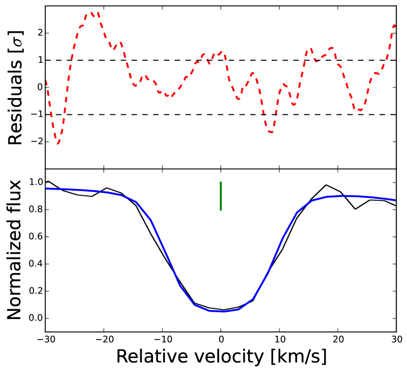
Figure 1: Top panel: normalized composite residual spectrum from 32 unblended and non-overlapping H₂ transitions. The dashed lines represent the $\pm 1\sigma$ boundaries. Bottom panel: the H₂ L3R(3) transition, with a rest wavelength of $\lambda^{0}=1067.5$ Å, is plotted as reference. The velocity scale is centred at the absorption redshift $z=2.33771$. The solid (blue) line shows the absorption model, while the solid (green) tick shows the position of the VC.

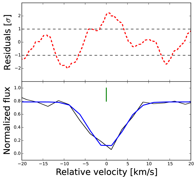
Figure 2: Top panel: normalized composite residual spectrum from 6 unblended and non-overlapping HD transitions. The dashed lines represent the $\pm 1\sigma$ boundaries. Bottom panel: the HD 7R(0) transition, with a rest wavelength of $\lambda^{0}=1021.5$ Å, is plotted as reference. The velocity scale is centred at the absorption redshift $z=2.33771$. The solid (blue) line shows the absorption model, while the solid (green) tick shows the position of the VC.

The parameters of the single VC model are presented in Table 3, while the complete absorption model is compared to the observed spectrum in Appendix A. The values of the H₂ column densities are in good agreement with those reported by Ivanchik et al. (2010), with only the rotational states with $J=2$ and 3 having a larger $N_{J}$ value, while the line width b presented here is smaller. The difference between the two b values may be explained by the fact that Ivanchik et al. (2010) derived their value from the curve of growth of rotational states with $J=2-5$, while the value presented in this work is derived considering the contribution from rotational states with $J<5$. The Doppler width parameter of the H₂ lines was observed to vary with the J-level (e.g. in HE0027–1836, Noterdaeme et al., 2007). According to Balashev et al. (2009), this can imply that the H₂ transitions with low J originate in the central part of the absorbing cloud, where the turbulence is minimal. On the other hand, high J transitions originate in the external part of the cloud, where larger turbulence may contribute more to the line broadening. As a consequence, the Doppler width derived only from the high-J states by Ivanchik et al. (2010) is larger than that reported here, which includes the contribution from the states with $J=0$ and 1. In Section 4.1.3 a test is performed to investigate the impact of the assumption of spatial homogeneity on the $\Delta\mu/\mu$ value derived in this work. The parameters describing the HD features are well in agreement with those reported by Ivanchik et al. (2010).

Table 3: Column densities $N_{J}$ and Doppler width b of the H₂ and HD transitions in the Q1232+082 spectrum.

Rotational level	$\log[N_{J}$/cm${}^{-2}]$	b [km s-1]
$J=0$	$19.41\pm 0.01$	$3.39\pm 0.06$
$J=1$	$19.26\pm 0.01$
$J=2$	$17.47\pm 0.04$
$J=3$	$17.16\pm 0.05$
$J=4$	$14.76\pm 0.02$
$J=5$	$14.23\pm 0.02$
HD $J=0$	$15.74\pm 0.53$	$1.67\pm 0.27$

4.1 Constraining $\Delta\mu/\mu$

As proposed by Thompson (1975), the H₂ absorption detected in high-redshift systems can be used to detect a temporal variation of the proton-to-electron mass ratio $\mu$. A variation of $\mu$ is reflected by a shift in the observed wavelength $\lambda^{z}_{i}$ of the i-th transition according to:

$$\lambda^{z}_{i}=\lambda^{0}_{i}(1+z_{\textrm{\scriptsize abs}})(1+K_{i}\frac{\Delta\mu}{\mu}),$$ (2)

where $\lambda^{0}_{i}$ is the rest wavelength of the transition, $z_{\textrm{\scriptsize abs}}$ is the absorption redshift, $\Delta\mu/\mu\equiv(\mu_{z}-\mu_{0})/\mu_{0}$ is the relative difference between the proton-to-electron mass ratio in the absorption system and the value measured on Earth, and $K_{i}$ is the sensitivity coefficient, defined as:

$$K_{i}\equiv\frac{\mathrm{d}\ln\lambda^{0}_{i}}{\mathrm{d}\ln\mu}.$$ (3)

The coefficient $K_{i}$ determines the sign and magnitude of the sensitivity to a varying $\mu$ and is specific for the i-th transition. The $K_{i}$ coefficients used in this work were calculated within a semi-empirical framework by Ubachs et al. (2007), including the effects beyond the Born-Oppenheimer approximation and are presented in Fig 3.

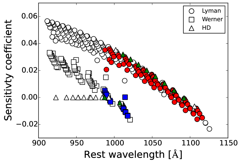
Figure 3: Sensitivity coefficients of Lyman and Werner transitions of H₂ and of HD transitions. The transitions considered in this analysis are marked with shaded markers.

The variation of $\mu$ is represented in vpfit by an extra free parameter. It was added to the other parameters ($N_{J}$, $z_{\textrm{\scriptsize abs}}$, b) of the H₂ and HD transitions only after having developed a robust absorption model. This fourth parameter was not added earlier in order to avoid that any flaw in the model itself would be compensated by an artificial variation of $\mu$. The model returned a value of the variation of the proton-to-electron mass ratio of $\Delta\mu/\mu=(22\pm 9_{stat})\times 10^{-6}$. It is worth noting that the statistical error was derived from the diagonal term of the final covariance matrix, representing thereby only the uncertainty arising from the S/N of the spectrum.

Ivanchik et al. (2002) derived two values for $\Delta\mu/\mu$ using the H₂ absorption in the system towards Q1232+082. They analyzed 12 isolated, unsaturated and unblended H₂ lines and used two independent sets of rest wavelengths $\lambda^{0}$ from Morton & Dinerstein (1976) and Abgrall et al. (1993) finding $\Delta\mu/\mu=(144\pm 114)\times 10^{-6}$ and $\Delta\mu/\mu=(132\pm 74)\times 10^{-6}$ respectively. The present analysis is based on $\sim 10$ times more lines, since the comprehensive fitting technique allows to fit partially overlapped and blended H₂ absorption features, and on more accurate rest wavelength measurements, which are considered exact for the purpose of comparison. This yielded a value of $\Delta\mu/\mu$ which is $\sim 10$ times more precise than that previously found for this system (Ivanchik et al., 2002).

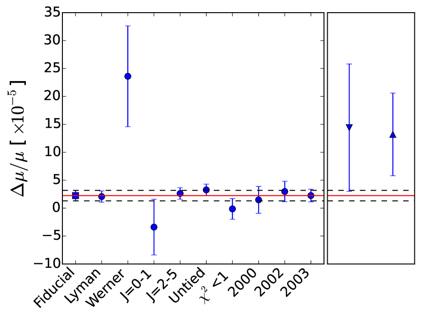
Figure 4: Left panel: Values of a varying $\mu$ obtained from the H₂ and HD absorption model, shown by a (blue) square, as well as from the consistency tests, shown by (blue) circles. The (red) solid line represents the fiducial $\Delta\mu/\mu$ value and the two dashed lines show its $\pm 1\sigma$ boundaries. Right panel: The (blue) upwards and downwards triangles represent the two measurements derived by Ivanchik et al. (2002) using the laboratory wavelengths reported by Morton & Dinerstein (1976) and Abgrall et al. (1993), respectively.

Following the same approach of Bagdonaite et al. (2014), a number of tests were performed to investigate the statistical robustness of the $\Delta\mu/\mu$ value, hereafter the fiducial value. In the following four sections, four different tests are presented along with their results, which are shown in Fig 4. Note that, in each test, the transitions that were not considered in the subset were included in the fit, but their $K_{i}$ coefficients were set to zero, i.e. they contributed to the absorption profile but not directly to a constraint on the $\Delta\mu/\mu$ parameter.

4.1.1 Isolating Lyman and Werner transitions

Previous studies showed that, since the H₂ sensitivity coefficients are wavelength-dependent, the presence of a distortion in the UVES wavelength scale would be nearly degenerate with a variation in $\mu$ (Ivanchik et al., 2005; Ubachs et al., 2007; Malec et al., 2010). This degeneracy will, in principle, be broken to some extent by fitting together the Lyman and the Werner transitions, since they have different sensitivity coefficients at similar rest wavelengths. The effect of such wavelength-dependent distortions can be investigated by separating the two H₂ band systems.

The two values returned are $\Delta\mu/\mu=(21\pm 10_{stat})\times 10^{-6}$ for the Lyman band systems and $\Delta\mu/\mu=(236\pm 90_{stat})\times 10^{-6}$ for the Werner band systems. The fact that the two values do not match within $2\sigma$ is considered as a hint of the presence of systematic effects. The shift between the Lyman-only and the Werner-only $\Delta\mu/\mu$ values requires a distortion slope which is $\sim 10$ times larger than what commonly found in UVES, hence it cannot be ascribed only to long-range distortions. This is considered evidence of an extra, unknown systematic effect which is affecting the fiducial value of $\Delta\mu/\mu$. The larger uncertainty on the value of $\Delta\mu/\mu$ delivered by the Werner transitions is ascribed to three effects: (i) the Werner transitions fall in the bluest part of the spectrum, which has a low S/N ($\sim 10$ per 2.5 km s^-1 per pixel at 3320 Å); (ii) the Werner transitions represent $\sim 16\%$ of the total number of H₂ transitions considered; (iii) the spread in the sensitivity coefficients of the Werner transitions, $\Delta K_{W}=0.02$, is lower than for Lyman transitions, $\Delta K_{L}=0.05$.

4.1.2 Isolating low and high J transitions

The impact of possible temperature inhomogeneities in the absorbing system on the constraint on $\Delta\mu/\mu$ was estimated by fitting the cold, low-J levels ($J<2$) and the hot, high-J levels ($J=2-5$) separately. This is possible because, due to the para-ortho distribution, the $J=1$ rotational state is significantly populated even at low temperatures, as discussed by Ubachs et al. (2007).

The two values derived from the cold and the warm transitions are $\Delta\mu/\mu=(-34\pm 50_{stat})\times 10^{-6}$ and $\Delta\mu/\mu=(26\pm 10_{stat})\times 10^{-6}$, respectively. The larger error on the measurement derived from the colder states can be explained from the fact that there are only 15 transitions with $J=0-1$ in the sample and they are nearly saturated, resulting in larger uncertainties on the position of the centroids of such absorption features. The two values match within their uncertainties, showing that the temperature inhomogeneities in the absorbing system do not significantly affect the constraint.

4.1.3 Untying free parameters among different J-levels

As discussed in Section 3, the present analysis was performed under the assumption that all the H₂ transitions share the same value of z and b. However, this may not be true if there is a spatial inhomogeneity in the absorbing cloud. In this case, transitions with different J-levels will arise under different physical conditions, which would be reflected by different values of their Doppler width b.

To test the validity of this assumption, a fit was run with the free parameters z and b untied among the different J-levels. The test returned $\Delta\mu/\mu=(5\pm 10_{stat})\times 10^{-6}$, which is in a good agreement with the fiducial value. As a consequence, the assumption of spatial homogeneity used in this analysis has almost no impact on the constraint on $\Delta\mu/\mu$.

4.1.4 Excluding problematic regions

Half of the selected spectral regions contain H₂ absorption features that show self-blending and overlap with intervening H i or narrow, unidentified absorption features that are likely to be metal absorption features. Such intervening lines were included in the fit, but they do not benefit from the strength of the comprehensive fitting method, since they cannot be tied in any way to other transitions. Hence, any flaw in modelling these lines will affect the fiducial value of $\Delta\mu/\mu$.

To test the impact of the unidentified intervening lines, a fit was performed considering only the 21 spectral regions that have a $\chi^{2}_{\nu}<1$. The fit returned a value of $\Delta\mu/\mu=(-1\pm 18)\times 10^{-6}$, which matches with the fiducial value within their uncertainties. It is concluded that the H₂ absorption model is robust enough not to be affected by flaws in the model of intervening neutral hydrogen and metal transitions.

4.1.5 Separating exposures from different periods

UVES is known to suffer from wavelength calibration distortions that are likely to originate in the internal settings of the instrument, as discussed in Section 5.1. Such distortions are likely to affect the fiducial value of $\Delta\mu/\mu$, hence quantifying this effect is crucial for any $\mu$ variation analysis. The attempt made to distortion-correct the spectrum is presented in Section 5.1, while here a test to estimate the consistency of the distortion slope across the observational programs is presented.

The final Q1232+082 spectrum was divided into 3 ‘subspectra’ – combined spectra formed from subsets of exposures – each comprising observations taken only in 2000, 2002, and 2003. Any change in the magnitude of the wavelength distortions would be reflected in a significant variation of the $\Delta\mu/\mu$ values derived from the subspectra. A value for $\Delta\mu/\mu$ was derived from each subspectrum, returning $\Delta\mu/\mu=(15\pm 24_{stat})\times 10^{-6}$ for exposures taken in 2000, $\Delta\mu/\mu=(30\pm 18_{stat})\times 10^{-6}$ for 2002, and $\Delta\mu/\mu=(22\pm 11_{stat})\times 10^{-6}$ for exposures taken in 2003. The differences in the errors among the values reflect the fact that the subsets do not have the same integration time, hence the S/N determining the statistical error changes among the subsets. The measurements agree well within their uncertainties, showing that the relative differences in the telescope settings among the different exposures do not significantly affect the fiducial value of $\Delta\mu/\mu$.

5 Systematic error

Following from Eq. (2), the measurable effect of a non-zero $\Delta\mu/\mu$ is a shift between molecular absorption features. As a consequence, any effect that introduces a distortion of the wavelength scale is likely to introduce a systematic error on the measured $\Delta\mu/\mu$ value. Note that this holds only for wavelength-dependent distortions, since any constant velocity offset will not cause any relative shift between the absorption features. Such a systematic will affect the resulting value for the absorption redshift parameter. The role of wavelength calibration errors as well as the spectral redispersion on the fiducial value of $\Delta\mu/\mu$ was studied in previous works on different systems (Malec et al., 2010; King et al., 2011; Bagdonaite et al., 2012, 2014; Daprà et al., 2015), while lack of attached ThAr calibrations was studied by Bagdonaite et al. (2012, 2014). In the following, the contributions to the systematic error budget from four sources of systematics are discussed following the same approach that was used in the aforementioned works.

5.1 Long-range distortions

The UVES spectrograph is known to suffer from wavelength calibration distortions. Long-range distortions were first detected by Rahmani et al. (2013) and, more recently, analyzed in further detail by Whitmore & Murphy (2015). Such distortions are likely to be due to a difference in the path the light from the quasar and from the calibration lamp travels within the instrument.

The supercalibration technique (Whitmore & Murphy, 2015) is a powerful method to correct the spectrum for the long-range distortions and was successfully applied to other systems (Bagdonaite et al., 2014; Daprà et al., 2015, 2016). It consists in a comparison of a spectrum taken with UVES with a reference spectrum from a Fourier Transform Spectrometer (FTS) solar spectrum, which has a more accurate frequency scale (Chance & Kurucz, 2010). Typical supercalibration targets are asteroids and ‘solar twin’ stars. The former have the same spectrum as the Sun since they reflect the solar light, while the latter are objects that show a spectrum which is almost identical to the solar one (Meléndez et al., 2009; Datson et al., 2014).

Since no supercalibration targets could be found in the ESO archive in a temporal window of $\sim 2$ weeks of the quasar exposures, the technique is not fully applicable to Q1232+082. However, the sparse sample reported by Whitmore & Murphy (2015) suggests that the UVES wavelength distortions might be quasi-stable in the period 2004-2008, with a distortion slope of $\sim 200$ m s^-1 per 1000 Å. Moreover, Whitmore & Murphy (2015) found one supercalibration target in 2001 delivering a distortion slope of $\sim 100$ m s^-1 per 1000 Å. Assuming that the distortions affecting UVES were stable in the period 2000-2003, the slope value of $\sim 100$ m s^-1 per 1000 Å was used to distortion-correct the Q1232+082 spectrum, delivering an updated fiducial $\Delta\mu/\mu$ value of $\Delta\mu/\mu=(19\pm 9_{stat})\times 10^{-6}$. An uncertainty on the distortion correction of $\pm 100$ m s^-1 per 1000 Å was estimated from the spread between the distortion slope values in 2001 and in the period 2004-2008. This translates into a systematic uncertainty on $\Delta\mu/\mu$ of $\sim 5\times 10^{-6}$ ($1\sigma$) and it was added to the systematic error budget. The presence of the long-range distortions with a positive distortion slope is found to push the $\Delta\mu/\mu$ value towards a more positive value, as was found in other systems (Rahmani et al., 2013; Bagdonaite et al., 2014, 2015; Daprà et al., 2015).

5.2 Intra-order distortions

At small scales, within single echelle orders, wavelength calibration distortions up to $\sim 100$ m s^-1 are expected in the spectra taken with UVES (Griest et al., 2010; Whitmore et al., 2010). However, since the H₂ transitions are spread over multiple echelle orders, such distortions are not expected to be dominant in the systematic error budget.

To estimate the impact of such intra-order distortions on $\Delta\mu/\mu$, a sawtooth wavelength distortion with an amplitude of $\pm 100$ m s^-1 was introduced in each echelle order before combining them together into the final quasar spectrum. A fit of the artificially distorted spectrum returned a value of $\Delta\mu/\mu=(22\pm 9)\times 10^{-6}$, which is well in agreement with the fiducial value before correcting for the long-range distortions. As a result, the intra-order distortions’ contribution to the systematic uncertainty is $<1\times 10^{-6}$, which is of the same order of that found in previous, similar studies on different systems (Malec et al., 2010; King et al., 2011; van Weerdenburg et al., 2011; Bagdonaite et al., 2014; Daprà et al., 2015). This effect, negligible compared to the uncertainty introduced by the long-range distortions, was included in the systematic error budget.

5.3 Lack of attached ThAr calibrations

The Q1232+082 spectra available in the ESO archive were recorded without the use of the attached ThAr calibration lamp exposure, hence they were calibrated using the standard ThAr calibration taken at the end of the night. Previous studies on different systems reported that the lack of attached ThAr calibrations introduces an error on the final value of $\Delta\mu/\mu$ which is $<1\times 10^{-6}$ (Bagdonaite et al., 2014; Daprà et al., 2015), which was added to the systematic error budget.

5.4 Spectral redispersion

The final Q1232+082 spectrum is composed by adding several exposures together. This procedure implies a redispersion of all the individual exposures on a common wavelength grid. The rebinning can cause flux correlations between neighbouring pixels, while the choice of the grid can distort the line-profile shapes affecting the value of $\Delta\mu/\mu$.

The impact of the spectral redispersion on $\Delta\mu/\mu$ was investigated by deriving a value of $\Delta\mu/\mu$ from six Q1232+082 spectra constructed using six different velocity grids in the range $2.47-2.53$ km s^-1 per pixel. The average deviation from the fiducial value is $1.4\times 10^{-6}$ and was included in the systematic uncertainty budget.

5.5 Total systematic uncertainty

The total systematic uncertainty on the fiducial value was derived by adding in quadrature all the contributions to the systematic error budget. The returned systematic error is $\sim 5\times 10^{-6}$, therefore the updated fiducial value becomes $\Delta\mu/\mu=(19\pm 9_{stat}\pm 5_{syst})\times 10^{-6}$.

6 Conclusions

A re-analysis of molecular hydrogen absorption at $z_{\textrm{\scriptsize abs}}\simeq 2.34$ towards quasar Q1232+082 is presented, in order to constrain a possible temporal variation of $\mu$ over cosmological time scales. The absorption system shows 106 H₂ and HD transitions associated with the DLA feature and spread over a range of $\sim 400$ Å. The dataset contains strongly saturated absorption features as well as overlaps with intervening lines. The comprehensive fitting technique used is able to handle such overlaps, as well as the partial coverage of the absorption system, whose respective effects are included in the absorption model. The H₂ and HD absorption was used to constrain a possible $\mu$-variation.

Since no supercalibration exposures are available for the Q1232+082 spectrum, an attempt to correct the spectrum for the long-range distortions was made based on the very sparely-sampled information from Whitmore & Murphy (2015). An estimate of the uncertainty on the distortion correction was made, based on the same sample, and it was added to the systematic error budget. The contributions to the systematic error budget from four different sources were investigated and the total systematic uncertainty was found to be dominated by the long-range wavelength distortions. The fiducial $\Delta\mu/\mu$ value delivered by the analysis is $\Delta\mu/\mu=(19\pm 9_{stat}\pm 5_{syst})\times 10^{-6}$.

This value is $\sim 10$ times more precise than those reported by Ivanchik et al. (2002). This is due to several improvements: (i) the comprehensive fitting technique applied here allows to expand the transition sample by including partially overlapped absorption features, (ii) the spectrum of Q1232+082 was built including two observational programs from 2003, that contribute additional $\sim 8$ hrs of integration, (iii) Ivanchik et al. (2002) used two sets of rest wavelengths with a low fractional accuracy, which is reflected in the uncertainty on the derived values of $\Delta\mu/\mu$. The updated fiducial value of $\Delta\mu/\mu$ presented in this work was derived using accurate rest wavelengths from laser spectroscopy (Hollenstein et al., 2006; Ivanov et al., 2008; Salumbides et al., 2008). Given the high accuracy of the studies, the rest wavelengths can be considered exact for the purpose of the comparison, (iv) the updated fiducial value of $\Delta\mu/\mu$ was derived after including a correction for the partial coverage in the H₂ absorption model.

The result presented here can be compared with other studies on different H₂ absorption systems, as shown in Fig. 5. The weighted mean of all the $\Delta\mu/\mu$ values considered results in a value of $\Delta\mu/\mu=(3.4\pm 1.6)\times 10^{-6}$, which is consistent with no variation over a look-back time of $\sim 10.5$-12.5 Gyrs at the $3\sigma$ level. It is noted that not all the measurements were corrected for the effect of wavelength distortions, which, for most cases, pushes the measured $\Delta\mu/\mu$ value towards more positive values by few parts per million. As a consequence, the averaged constraint should be considered as an upper limit to the temporal variation of $\mu$ over cosmological timescales.

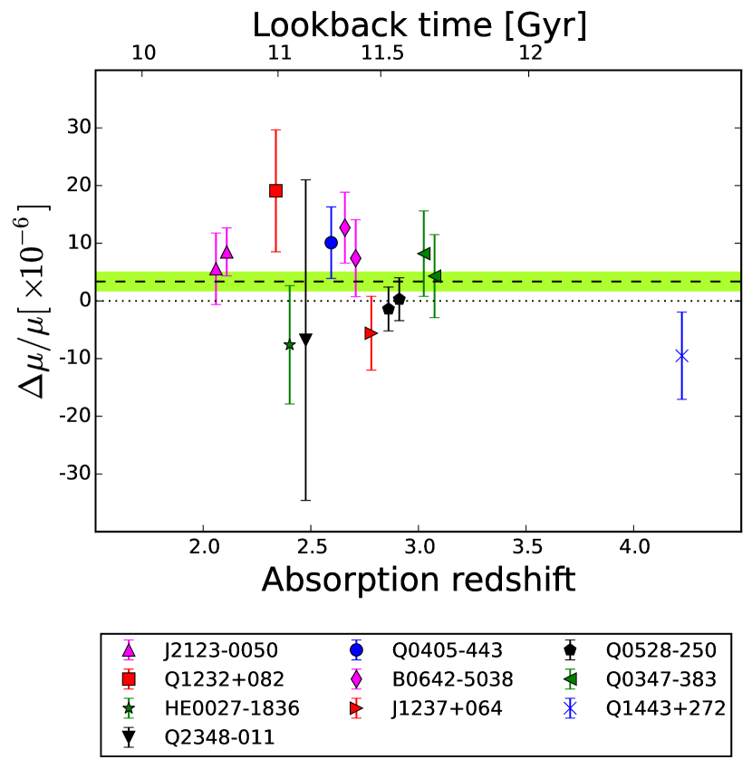
Figure 5: Measurements of $\Delta\mu/\mu$ derived from molecular hydrogen absorbing systems. The value presented here is shown with a (red) square. The other values of $\Delta\mu/\mu$ were derived from systems: J2123-0050 (Malec et al., 2010; van Weerdenburg et al., 2011), HE0027-1836 (Rahmani et al., 2013), Q2348-011 (Bagdonaite et al., 2012), Q0405-443 (King et al., 2008), B0642-5038 (Albornoz Vásquez, D. et al., 2014; Bagdonaite et al., 2014), J1237+0647 (Daprà et al., 2015, 2016), Q0528-250 (King et al., 2008; King et al., 2011), Q0347-383 (King et al., 2008; Wendt & Molaro, 2012) and Q1443+272 (Bagdonaite et al., 2015). Note that multiple $\Delta\mu/\mu$ measurements were derived from systems J2123-0050, B0642-5038, Q0528-250 and Q0347-383, and are presented with an offset of $+0.05$ on the x axis to avoid overlaps. The dashed line represents the weighted mean of all the values, the shaded area shows its $\pm 1\sigma$ boundaries, and the dotted line represents the zero level.

A list of the known systems showing H₂ and/or CO absorption was compiled by Ubachs et al. (2016). The ten best absorbers for a $\mu$ variation analysis, because of their brightness, with a Bessel $R_{mag}\leq 18.4$, and H₂ column density, $\log N_{H_{2}}\geq 14.5$, are shown in Fig. 5. With the analysis presented here, we complete a set of the ten best absorbers for $\mu$ variation. Note that the set does not contain the system Q2100–0641 at $z_{\textrm{\scriptsize abs}}=3.09$, which has $R_{mag}=17.52$ and $\log N_{H_{2}}=18.76$ (Balashev et al., 2015), and could represent a good target for future investigations.

The current constraint on $\Delta\mu/\mu$ is almost equally limited by statistical and systematic uncertainties. While the former can be improved by increasing the S/N, the latter is dominated by the long-range wavelength distortions. Such distortions affects not only UVES, but also the High Resolution Echelle Spectrograph, HIRES, mounted on the Keck telescope, which is the other instrument used to investigate a temporal drift of $\mu$. Whitmore & Murphy (2015) expanded and refined the supercalibration technique to distortion-correct the quasar spectra, and they showed that the long-range distortions are ubiquitous across the entire UVES and HIRES history. The fact that most of the archival exposures do not have any attached supercalibration precludes a significant reduction in the systematic error on $\Delta\mu/\mu$ when using such data from these spectrographs.

The current constraint on a varying $\mu$ can be improved with the new generation of high resolution spectrographs, like the upcoming Echelle SPectrograph for Rocky Exoplanet and Stable Spectroscopic Observations (ESPRESSO, Pepe et al., 2010). ESPRESSO, that has a resolution $\sim 3$ times higher than the one used in this work, and is able to resolve VCs with a Doppler broadening parameter as narrow as $\sim 1.0$ km s^-1. Moreover, being immune, in principle, to the long-range wavelength distortions, thanks to its fibre feed and frequency-comb wavelength calibration, it will deliver constraints on $\Delta\mu/\mu$ with smaller systematic uncertainties. However, ESPRESSO will not cover wavelengths shorter than $\sim 3800$ Å, which means it can only target H₂ absorption lines in systems at $z_{\textrm{\scriptsize abs}}>2.4$, and very few such systems are known towards bright quasars (Ubachs et al., 2016).

Appendix A Absorption model

Figures 6-13 show the H₂ absorption model in the spectrum of the absorbing system at $z_{\textrm{\scriptsize abs}}\simeq 2.34$ towards quasar Q1232+082.

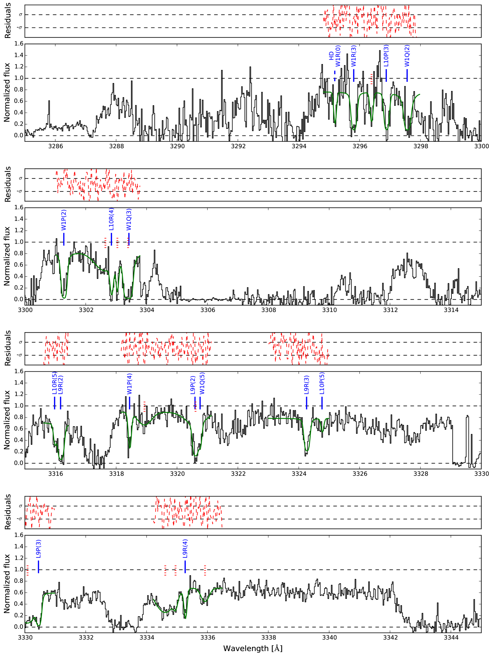
Figure 6: Spectrum of quasar Q1232+082 (part 1 of 8). The H₂ absorption model is represented with a (green) solid line. H₂ transitions are shown with (blue) solid ticks, HD transitions with (blue) dashed ticks, and the (red) dotted ticks show the position of the intervening H I and metal lines.

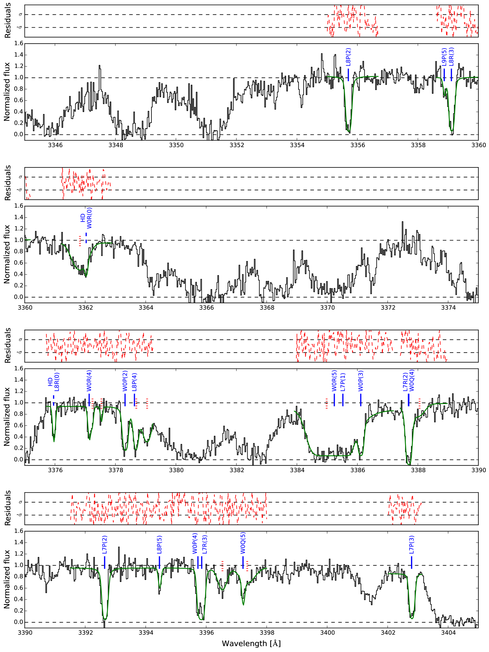
Figure 7: Spectrum of quasar Q1232+082 (part 2 of 8), continued.

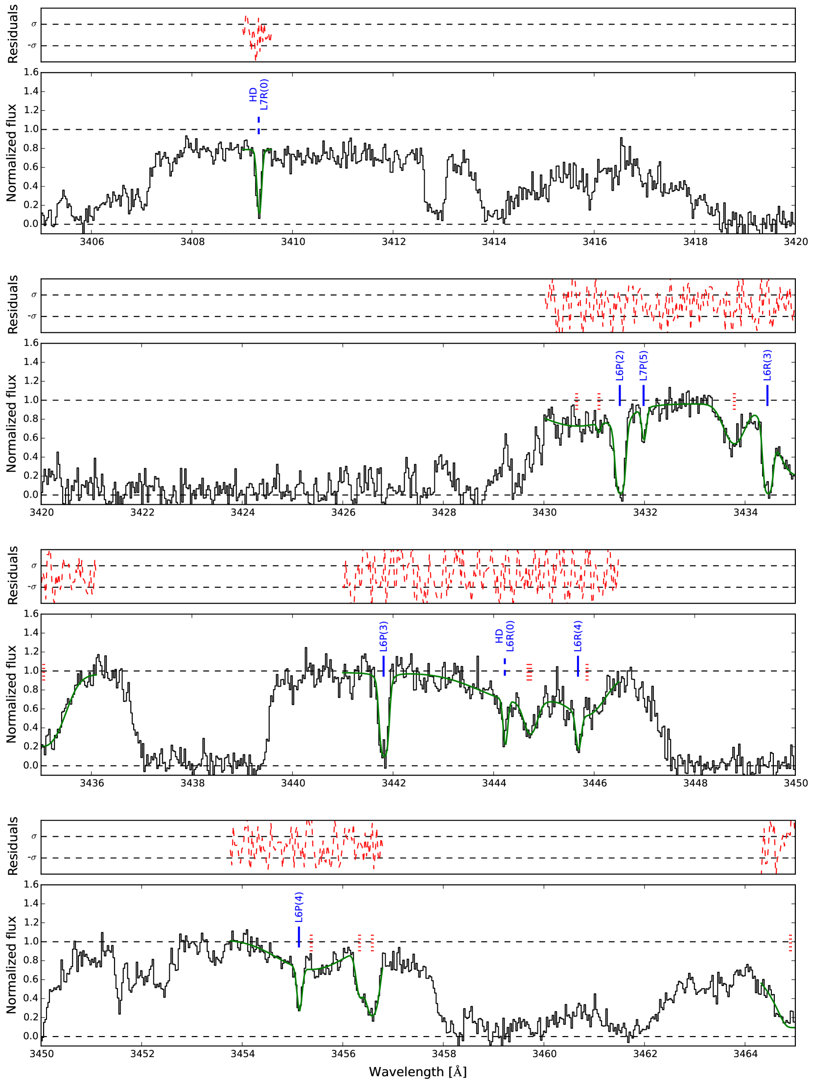
Figure 8: Spectrum of quasar Q1232+082 (part 3 of 8), continued.

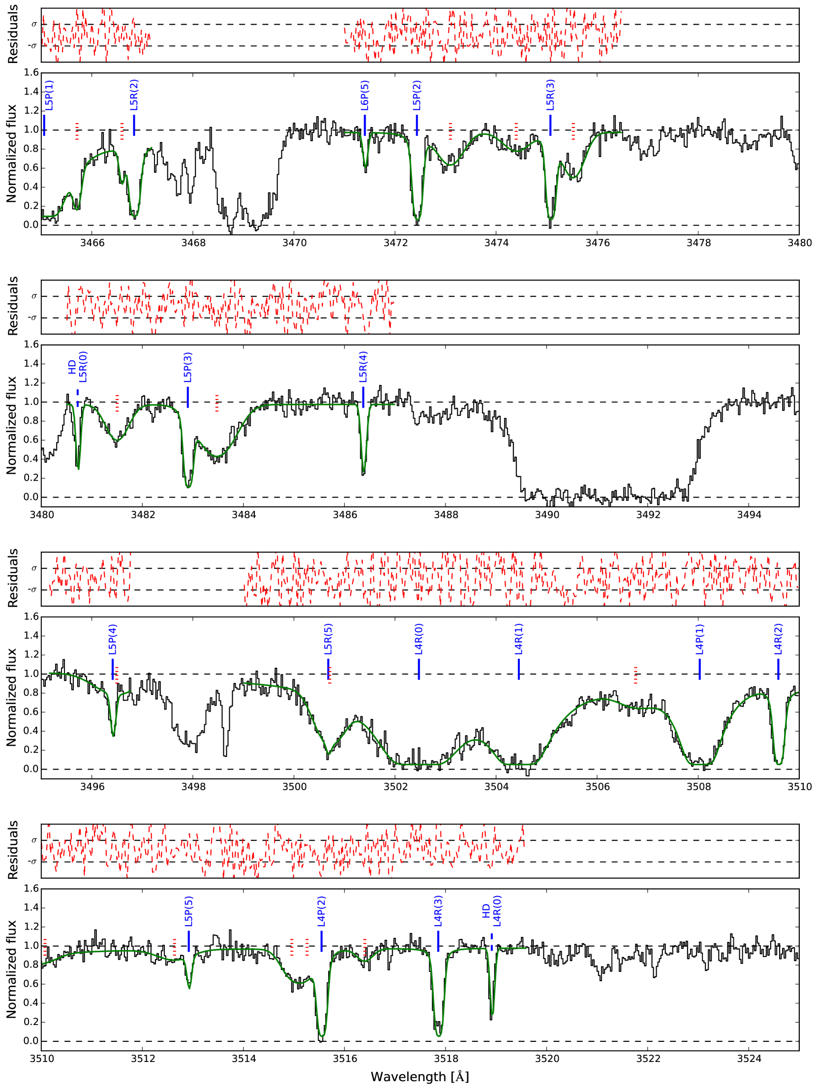
Figure 9: Spectrum of quasar Q1232+082 (part 4 of 8), continued.

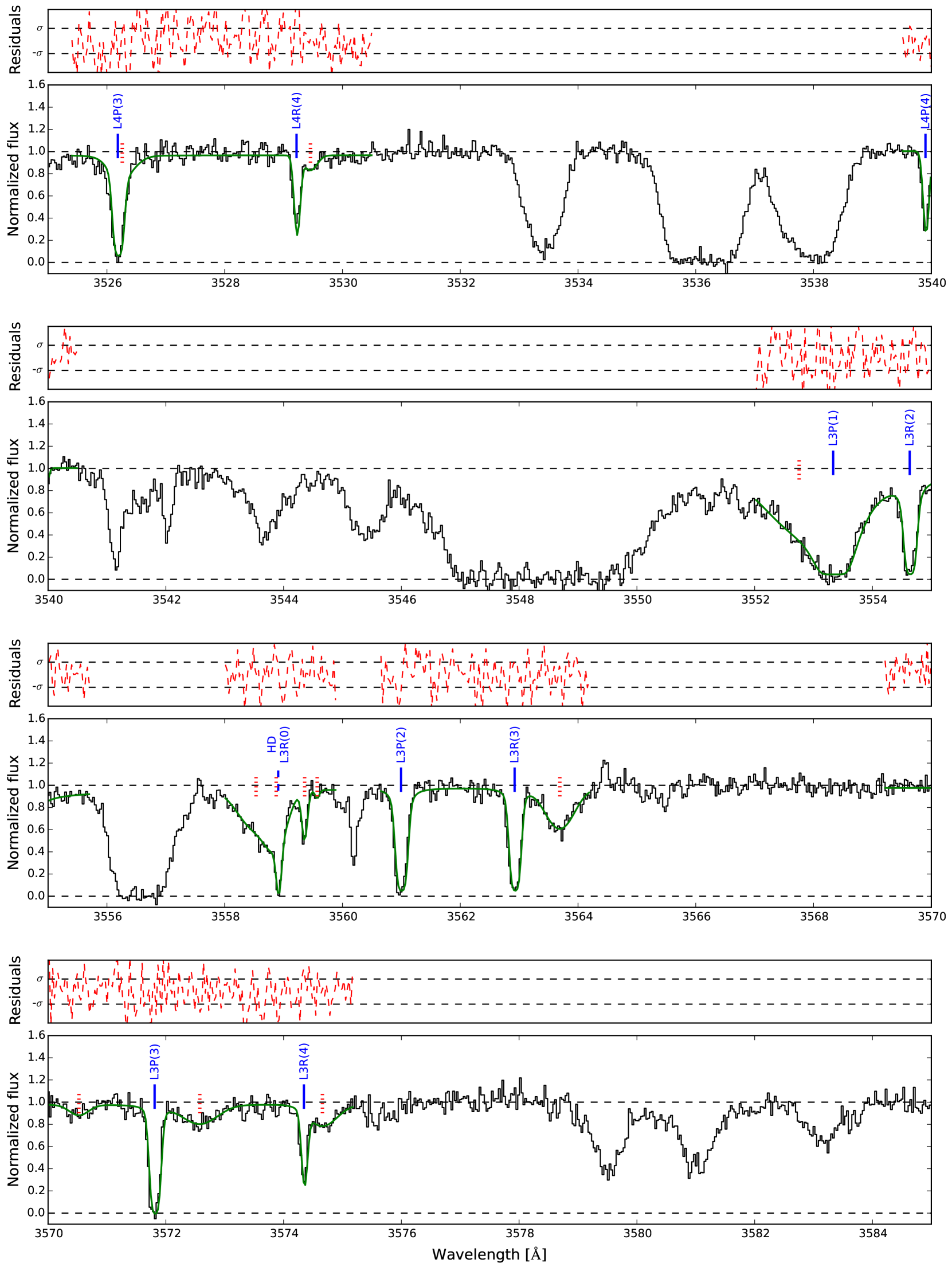
Figure 10: Spectrum of quasar Q1232+082 (part 5 of 8), continued.

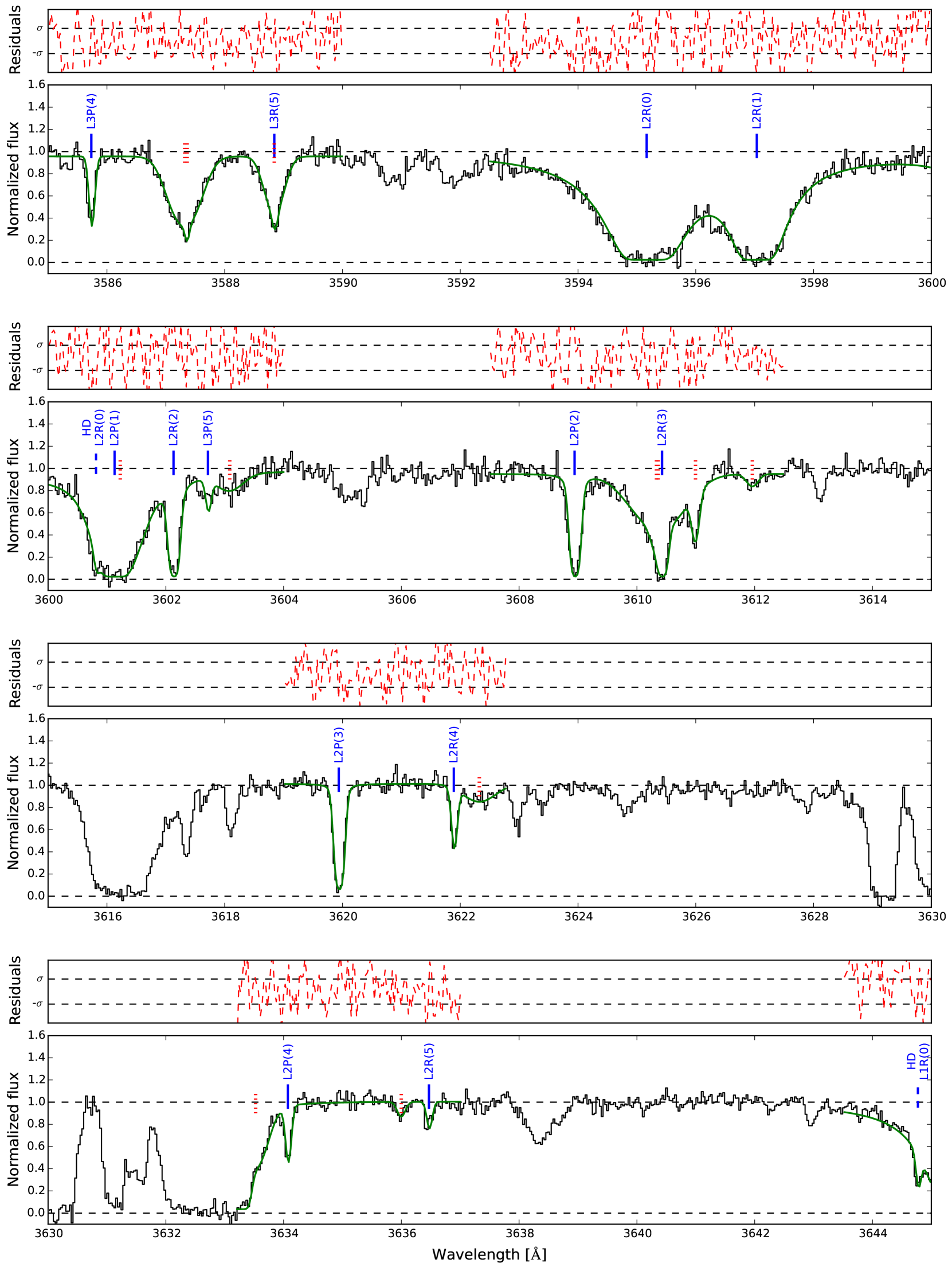
Figure 11: Spectrum of quasar Q1232+082 (part 6 of 8), continued.

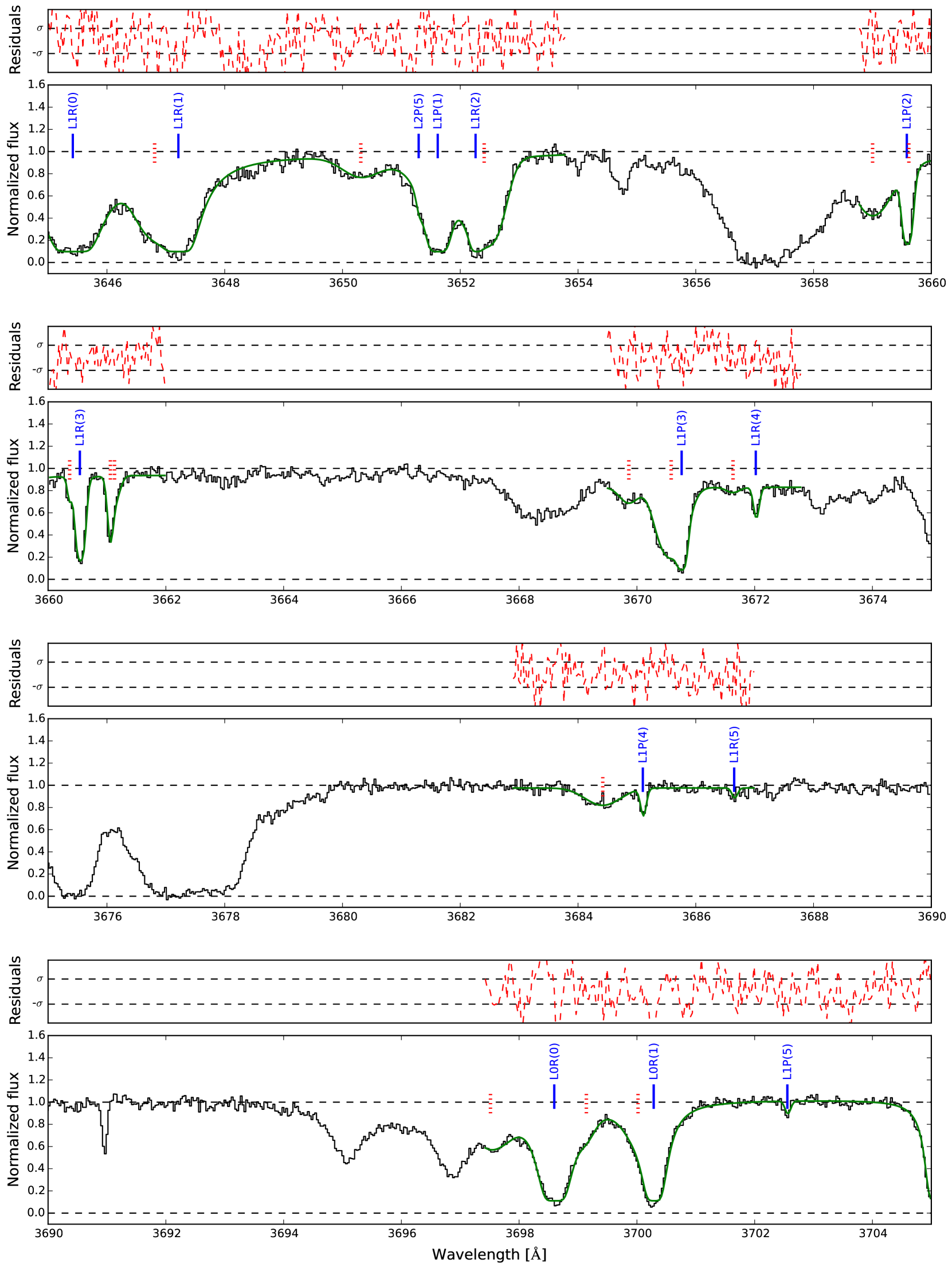
Figure 12: Spectrum of quasar Q1232+082 (part 7 of 8), continued.

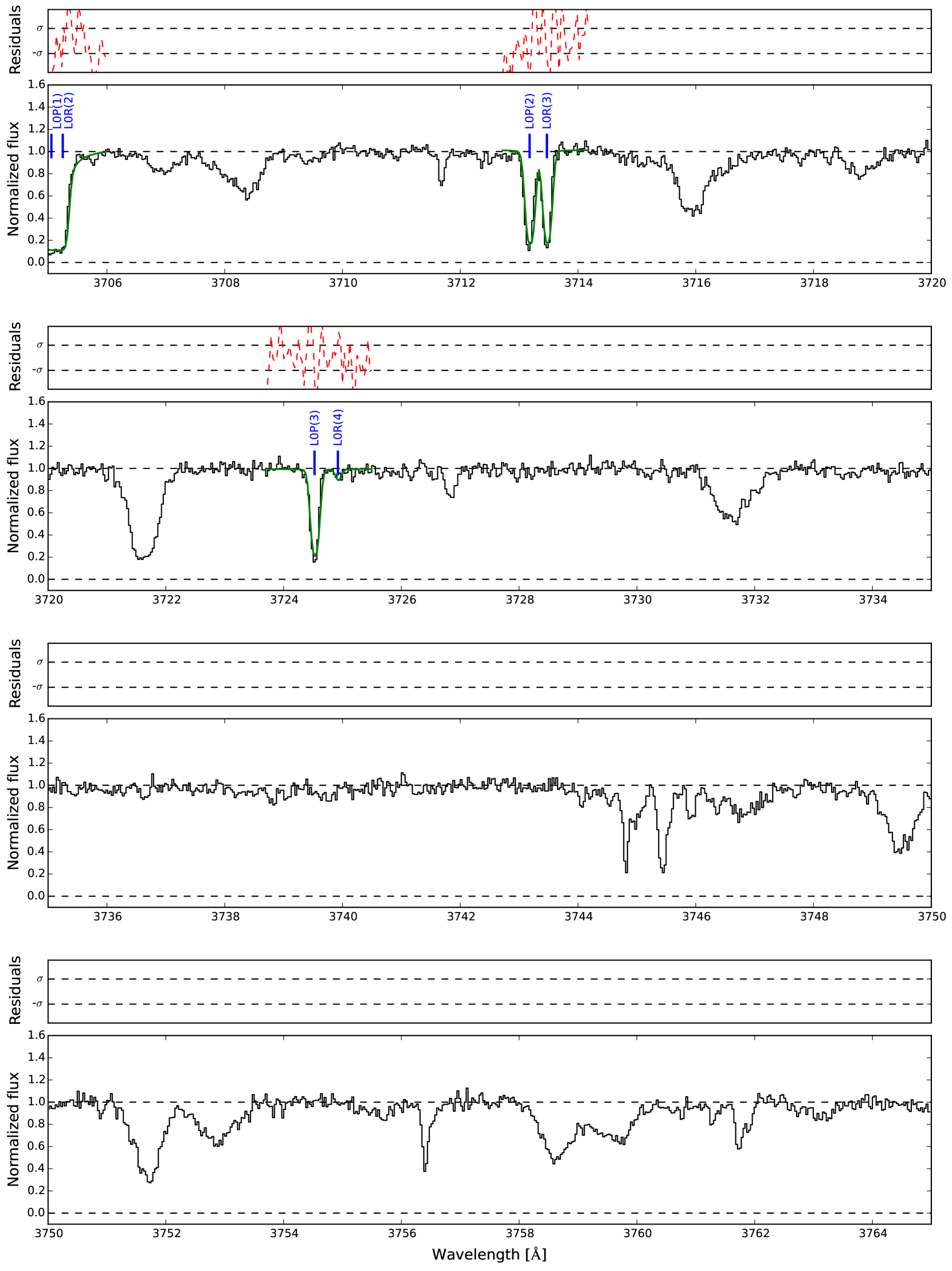
Figure 13: Spectrum of quasar Q1232+082 (part 8 of 8), continued.

References

- Abgrall & Roueff (2006) Abgrall H., Roueff E., 2006, A&A, 445, 361
- Abgrall et al. (1993) Abgrall H., Roueff E., Launay F., Roncin J. Y., Subtil J. L., 1993, J. Mol. Spectrosc., 157, 512
- Abgrall et al. (1994) Abgrall H., Roueff E., Launay F., Roncin J.-Y., 1994, Can. J. Phys., 72, 856
- Abgrall et al. (2000) Abgrall H., Roueff E., Drira I., 2000, A&AS, 141, 297
- Akaike (1974) Akaike H., 1974, IEEE Trans. Aut. Contr., 19, 716
- Albornoz Vásquez, D. et al. (2014) Albornoz Vásquez, D. Rahmani, H. Noterdaeme, P. Petitjean, P. Srianand, R. Ledoux, C. 2014, A&A, 562, A88
- Bagdonaite et al. (2012) Bagdonaite J., Murphy M. T., Kaper L., Ubachs W., 2012, MNRAS, 421, 419
- Bagdonaite et al. (2013a) Bagdonaite J., Daprà M., Jansen P., Bethlem H. L., Ubachs W., Muller S., Henkel C., Menten K. M., 2013a, Phys. Rev. Lett., 111, 231101
- Bagdonaite et al. (2013b) Bagdonaite J., Jansen P., Henkel C., Bethlem H. L., Menten K. M., Ubachs W., 2013b, Science, 339, 46
- Bagdonaite et al. (2014) Bagdonaite J., Ubachs W., Murphy M. T., Whitmore J. B., 2014, ApJ, 782, 10
- Bagdonaite et al. (2015) Bagdonaite J., Ubachs W., Murphy M. T., Whitmore J. B., 2015, Phys. Rev. Lett., 114, 071301
- Balashev et al. (2009) Balashev S. A., Varshalovich D. A., Ivanchik A. V., 2009, Astron. Lett., 35, 150
- Balashev et al. (2011) Balashev S. A., Petitjean P., Ivanchik A. V., Ledoux C., Srianand R., Noterdaeme P., Varshalovich D. A., 2011, MNRAS, 418, 357
- Balashev et al. (2015) Balashev S. A., Noterdaeme P., Klimenko V. V., Petitjean P., Srianand R., Ledoux C., Ivanchik A. V., Varshalovich D. A., 2015, A&A, 575, L8
- Carswell & Webb (2014) Carswell R. F., Webb J. K., 2014, VPFIT: Voigt profile fitting program, Astrophysics Source Code Library (ascl:1408.015)
- Chance & Kurucz (2010) Chance K., Kurucz R. L., 2010, J. Quant. Spectrosc. Radiat. Transfer, 111, 1289
- Daprà et al. (2015) Daprà M., Bagdonaite J., Murphy M. T., Ubachs W., 2015, MNRAS, 454, 489
- Daprà et al. (2016) Daprà M., Niu M. L., Salumbides E. J., Murphy M. T., Ubachs W., 2016, ApJ, 826, 192
- Datson et al. (2014) Datson J., Flynn C., Portinari L., 2014, MNRAS, 439, 1028
- Ge & Bechtold (1999) Ge J., Bechtold J., 1999, in Carilli C. L., Radford S. J. E., Menten K. M., Langston G. I., eds, ASP Conf. Ser. Vol. 156, Highly Redshifted Radio Lines. p. 121
- Griest et al. (2010) Griest K., Whitmore J. B., Wolfe A. M., Prochaska J. X., Howk J. C., Marcy G. W., 2010, ApJ, 708, 158
- Henkel et al. (2005) Henkel C., Jethava N., Kraus A., Menten K. M., Carilli C. L., Grasshoff M., Lubowich D., Reid M. J., 2005, A&A, 440, 893
- Henkel et al. (2008) Henkel C., Braatz J. A., Menten K. M., Ott J., 2008, A&A, 485, 451
- Hollenstein et al. (2006) Hollenstein U., Reinhold E., de Lange C. A., Ubachs W., 2006, J. Phys. B, 39, L195
- Ivanchik et al. (2002) Ivanchik A. V., Rodriguez E., Petitjean P., Varshalovich D. A., 2002, Astron. Lett., 28, 423
- Ivanchik et al. (2005) Ivanchik A., Petitjean P., Varshalovich D., Aracil B., Srianand R., Chand H., Ledoux C., Boissé P., 2005, A&A, 440, 45
- Ivanchik et al. (2010) Ivanchik A. V., Petitjean P., Balashev S. A., Srianand R., Varshalovich D. A., Ledoux C., Noterdaeme P., 2010, MNRAS, 404, 1583
- Ivanov et al. (2008) Ivanov T. I., Roudjane M., Vieitez M. O., de Lange C. A., Tchang-Brillet W.-Ü. L., Ubachs W., 2008, Phys. Rev. Lett., 100, 093007
- Ivanov et al. (2010) Ivanov T. I., Dickenson G. D., Roudjane M., Oliveira N. D., Joyeux D., Nahon L., Tchang-Brillet W.-U. L., Ubachs W., 2010, Mol. Phys., 108, 771
- Jansen et al. (2014) Jansen P., Bethlem H. L., Ubachs W., 2014, J. Chem. Phys., 140, 010901
- Kanekar (2011) Kanekar N., 2011, ApJ, 728, L12
- Kanekar et al. (2015) Kanekar N., et al., 2015, MNRAS, 448, L104
- King et al. (2008) King J. A., Webb J. K., Murphy M. T., Carswell R. F., 2008, Phys. Rev. Lett., 101, 251304
- King et al. (2011) King J. A., Murphy M. T., Ubachs W., Webb J. K., 2011, MNRAS, 417, 3010
- Kozlov & Levshakov (2013) Kozlov M. G., Levshakov S. A., 2013, Ann. Phys., 525, 452
- Malec et al. (2010) Malec A. L., et al., 2010, MNRAS, 403, 1541
- Meléndez et al. (2009) Meléndez J., Asplund M., Gustafsson B., Yong D., 2009, ApJ, 704, L66
- Morton & Dinerstein (1976) Morton D. C., Dinerstein H. L., 1976, ApJ, 204, 1
- Muller et al. (2011) Muller S., et al., 2011, A&A, 535, A103
- Murphy (2016) Murphy M. T., 2016, UVES_popler: POst-PipeLine Echelle Reduction software, doi:10.5281/zenodo.44765, http://dx.doi.org/10.5281/zenodo.44765
- Murphy et al. (2008) Murphy M. T., Flambaum V. V., Muller S., Henkel C., 2008, Science, 320, 1611
- Noterdaeme et al. (2007) Noterdaeme P., Petitjean P., Srianand R., Ledoux C., Le Petit F., 2007, A&A, 469, 425
- Pepe et al. (2010) Pepe F. A., et al., 2010, in Society of Photo-Optical Instrumentation Engineers (SPIE) Conference Series. p. 9, doi:10.1117/12.857122
- Rahmani et al. (2013) Rahmani H., et al., 2013, MNRAS, 435, 861
- Salumbides et al. (2008) Salumbides E. J., Bailly D., Khramov A., Wolf A. L., Eikema K. S. E., Vervloet M., Ubachs W., 2008, Phys. Rev. Lett., 101, 223001
- Srianand et al. (2000) Srianand R., Petitjean P., Ledoux C., 2000, Nature, 408, 931
- Thompson (1975) Thompson R. I., 1975, Astrophys. Lett., 16, 3
- Ubachs et al. (2007) Ubachs W., Buning R., Eikema K. S. E., Reinhold E., 2007, J. Mol. Spectrosc., 241, 155
- Ubachs et al. (2016) Ubachs W., Bagdonaite J., Salumbides E. J., Murphy M. T., Kaper L., 2016, Rev. Mod. Phys., 88, 021003
- Uzan (2011) Uzan J.-P., 2011, Living Rev. Relat., 14, 2
- Varshalovich & Levshakov (1993) Varshalovich D. A., Levshakov S. A., 1993, Sov. J. Exp. Theor. Phys., 58, 237
- Varshalovich et al. (2001) Varshalovich D. A., Ivanchik A. V., Petitjean P., Srianand R., Ledoux C., 2001, Astron. Lett., 27, 683
- Wendt & Molaro (2012) Wendt M., Molaro P., 2012, A&A, 541, A69
- Whitmore & Murphy (2015) Whitmore J. B., Murphy M. T., 2015, MNRAS, 447, 446
- Whitmore et al. (2010) Whitmore J. B., Murphy M. T., Griest K., 2010, ApJ, 723, 89
- van Weerdenburg et al. (2011) van Weerdenburg F., Murphy M. T., Malec A. L., Kaper L., Ubachs W., 2011, Phys. Rev. Lett., 106, 180802