A physically-based model of the ionizing radiation from active galaxies for photoionization modeling
Abstract
We present a simplified model of Active Galactic Nucleus (AGN) continuum emission designed for photoionization modeling. The new model oxaf reproduces the diversity of spectral shapes that arise in physically-based models. We identify and explain degeneracies in the effects of AGN parameters on model spectral shapes, with a focus on the complete degeneracy between the black hole mass and AGN luminosity. Our re-parametrized model oxaf removes these degeneracies and accepts three parameters which directly describe the output spectral shape: the energy of the peak of the accretion disk emission , the photon power-law index of the non-thermal emission , and the proportion of the total flux which is emitted in the non-thermal component . The parameter is presented as a function of the black hole mass, AGN luminosity, and ‘coronal radius’ of the optxagnf model upon which oxaf is based. We show that the soft X-ray excess does not significantly affect photoionization modeling predictions of strong emission lines in Seyfert narrow-line regions. Despite its simplicity, oxaf accounts for opacity effects where the accretion disk is ionized because it inherits the ‘color correction’ of optxagnf. We use a grid of mappings photoionization models with oxaf ionizing spectra to demonstrate how predicted emission-line ratios on standard optical diagnostic diagrams are sensitive to each of the three oxaf parameters. The oxaf code is publicly available in the Astrophysics Source Code Library.
Subject headings:
black hole physics — galaxies: individual (NGC 1365 (catalog )) — ISM: lines and bands — line: formation — quasars: emission lines1. Introduction
Active galactic nuclei (AGN) feature narrow-line regions (NLRs) in which continuum radiation from the central engine photoionizes the surrounding interstellar medium (ISM). The relatively hard AGN continuum emission injects more energy and photoionizes the ISM to higher ionization states than the ionizing spectra of OB stars at the centers of H II regions.
Many insights into the physics of the the ISM in active galaxies have been gained through the use of photoionization models. The results of photoionization modeling facilitate the routine diagnosis of the density, temperature, and cause of ionization of NLR gas from observed emission-line spectra. Photoionization models have been used to explain the very similar NLR ionization parameters observed across the population of active galaxies - this effect is caused by the gas pressure gradient balancing the radiation pressure gradient in dusty NLR clouds such that the ‘local’ ionization parameter is self-regulated (Dopita et al., 2002; Groves et al., 2004). Models are an important tool in investigating the effects of various ISM parameters on emission-line spectra; e.g. determining the effects of changing abundances (Groves et al., 2006). Recently, Davies et al. (2016) showed how comparisons between models and spatially-resolved spectroscopy may reveal where extended NLRs are radiation pressure-dominated or gas pressure-dominated on scales of tens to hundreds of parsecs.
The emission line spectra of NLRs in active galaxies strongly depend upon the shape of the spectrum of the central source at energies immediately above the Lyman limit at 13.6 eV. These ionizing photons are not directly observable because they are very strongly absorbed in the NLR and broader ISM of the host galaxy, as well as in the ISM of the Milky Way.
Up to the present, ionizing AGN spectra for photoionization modeling have almost exclusively been constructed using piecewise functions of one to three simple power-laws (e.g. Viegas-Aldrovandi & Contini, 1989; Murayama & Taniguchi, 1998; Allen et al., 1998; Evans et al., 1999; Contini & Viegas, 2001; Collins et al., 2009). Groves et al. (2004) use a conventional range of power-law indices of to , for a single power-law covering 0.005 to 1 keV. The authors find that a steeper power-law leads to weaker high-ionization lines and relatively stronger H lines, due to the relative excess of H- but not He-ionizing photons. A more physically-motivated empirical two-component model for the ionizing spectrum is used, for example, in Bland-Hawthorn et al. (2013)).
In this work we seek to develop a modern AGN continuum emission model for use as the input spectrum in photoionization models, based on physically-derived models, and including for example ionization effects in the shape of the accretion disk spectrum. We aim to identify the important AGN parameters which influence the shape of the ionizing spectrum and hence the predicted emission-line ratios. This allows us to minimize the parameter space used to cover a large range of model spectra. A small parameter space is easier to handle conceptually and computationally, and the process of combining fully and partially degenerate parameters into a smaller set of parameters results in insights into how the shape of the ionizing spectrum may arise from various combinations of fundamental AGN parameters.
In photoionization modeling we assume that the model ionizing spectrum will be intrinsic when it reaches the modeled clouds, i.e. that there is no significant absorption between the central engine and the modeled clouds. Hence the spectra will primarily feature a peak formed by a superposition of pseudo-blackbodies due to the accretion disk, and a power-law non-thermal component resulting from Compton up-scattering of disk photons. A physical model of these spectra may be expected to be well-described by few parameters.
A detailed model of continuum emission from AGN must rely on theoretical emissivities from accretion disk models. The standard Novikov-Thorne ‘thin disk’ accretion model (Novikov & Thorne (1973), building on the work of Shakura & Sunyaev (1973)) is applicable over much of the accretion rate regime of Seyfert galaxies ( to ). This model has parameters such as the SMBH mass, spin, and accretion rate, which influence the theoretical ionizing AGN spectrum.
Understanding how the key parameters control the shape of the ionizing EUV-soft X-ray spectrum of AGN allows us to produce a model which keeps the number of free parameters to a minimum. Our simplified spectral modeling is, however, based firmly on the optxagnf model (Done et al., 2012; Jin et al., 2012a, b, c). We chose this model because it is a recent, widely-used model, it calculates theoretical spectra using physics such as the Novikov-Thorne thin accretion disk model, and because it uses a ‘color temperature correction’ which accounts for electron-scattering opacity in parts of the disk where hydrogen is ionized. The optxagnf model provides the basis for a new physically-based model of the ionizing AGN spectrum for photoionization modeling.
In photoionization modeling, the ionization parameter and density are important input parameters, so the flux incident on the model cloud is easily calculated. However the actual luminosity of the ionizing source is important only if the modeler is interested in determining the distance of the modeled cloud from the source. We are primarily concerned with the shape of the ionizing spectrum, because this determines the relative emission-line fluxes. Any parameter redundancies may render more difficult the interpretation of the NLR spectrum caused by a given AGN ionizing spectrum. In this work we identify and explain various spectral-shape degeneracies, such as the complete degeneracy between the black hole mass and luminosity in the Novikov-Thorne emissivity, and successfully remove the degeneracies by constructing a new model.
We simplify the optxagnf model by carefully removing and merging degenerate parameters. The resulting model, oxaf, satisfies our requirements by generating realistic model spectral shapes using the fewest possible parameters, and with all of the parameters having a direct impact on the shape of the model spectrum. We then investigate the effect of the oxaf parameters on photoionization models of NLR clouds.
In Section 2 we describe the spectral-shape degeneracies that arise in the thin-disc accretion model and in the the optxagnf model, and in Section 3 we describe the parameters used to re-parametrize optxagnf. In Section 4 we explain how these parameters are used to construct our simplified model oxaf and describe the implementation and validation of the new model. In Section 5 we explore how the oxaf parameters affect photoionization model predictions for diagnostic emission lines. Our conclusions are presented in Section 6.
2. Relationships between parameters in AGN spectral models
The unified model of AGN describes a central, accreting supermassive black hole (SMBH) surrounded by a broad line region, a dusty obscuring torus, and a narrow-line region (Antonucci, 1993). The powerful continuum radiation from the central accretion structure illuminates the broad and narrow-line regions.
Important parameters which determine the spectrum of the central accretion structure are the Eddington ratio , the SMBH mass , the dimensionless SMBH spin , and the innermost radius at which the disk is directly visible. In this section we describe the effects of these parameters on the shape of the ionizing spectrum and the relationships between the parameters.
2.1. The relationship between the SMBH mass and Eddington rate
The Novikov-Thorne thin disk model produces a clean relationship between and , with these parameters having the same effect on the model spectral shape.
The temperature at a given radius of the accretion disk may be calculated using the following equation for the ‘outer’ region of the disk (Equation 5.10.1 in Novikov & Thorne, 1973):
| (1) |
where is the black hole mass, is the accretion rate, is the dimensionless spin parameter, is the Stefan-Boltzmann constant, and is the gravitational constant. With defined as the radius normalized by the gravitational radius (; = ), the quantities , and are complicated dimensionless radial functions associated with relativistic corrections in the analytic accretion disk solution of Novikov & Thorne (1973) (the function was presented in the follow-up work of Page & Thorne (1974); , and tend to 1 at large ).
Using where is the total accretion efficiency, and with the definition of given above, Equation 1 may be rewritten as
| (2) |
where is a collection of physical and numerical constants and .
Inverting Equation 2, we find that
| (3) |
for a function , since . Specifying the temperature at a particular normalized radius as well as the spin uniquely determines the ratio such that the parameters and are degenerate in their effects on the spectral shape.
2.2. The optxagnf model
The optxagnf model (Done et al., 2012; Jin et al., 2012a, b, c) is a significant effort in the development of theoretical models of continuum radiation from accretion onto black holes that match observed optical, UV and X-ray continuum spectra. The model is available for use with the xspec spectral fitting package, under the name optxagnf.
The model aims to capture the essential features of the continuum emission from a relativistic thin accretion disk with a Comptonizing corona in the equatorial plane of a rotating black hole. It is assumed that material is accreted only through the outer disk, and the released gravitational energy is divided between three spectral components:
-
•
A pseudo-thermal accretion disk component
-
•
A high-energy, power-law non-thermal component, formed by Compton up-scattering from an optically thin, high-temperature medium
-
•
An intermediate (‘soft X-ray excess’) component formed by Compton up-scattering from a Compton-thick, low-temperature medium
The model implements the following:
-
•
The standard Novikov & Thorne (1973) thin-disk relativistic accretion disk emissivity
-
•
A disk spectrum produced by summing blackbodies in successive annuli, with the temperature of the blackbody spectrum corrected if necessary using an empirical color temperature correction . The correction is required due to the absorption opacity varying with temperature, density and wavelength; in particular it is used where hydrogen is ionized in the inner parts of the disk in an attempt to account for modifications to the spectrum due to the disk not being locally thermalized and due to electron-scattering opacity (Davis et al., 2006). The correction becomes increasingly important as the temperature of the disk increases (as the luminosity increases or black hole mass decreases).
-
•
The disk luminosity between the innermost stable circular orbit and , the ‘coronal radius’, is all emitted as Comptonized radiation.
-
•
The Comptonized radiation is split between the soft, intermediate component (assumed to arise in the accretion structure itself) and the hard X-ray power-law tail. The seed photons for Comptonization in both cases come from a blackbody with the same (corrected) temperature as the disk at .
-
•
The total luminosity from all three components of the emission (disk, Comptonized soft X-ray excess, Comptonized hard X-ray tail) is fixed by the accretion rate and SMBH spin.
The following are the parameters required by optxagnf to characterize the various physical components of the model:
-
•
, the black hole mass
-
•
, the AGN luminosity in units of the Eddington luminosity, which is proportional to .
-
•
, the dimensionless black hole rotation parameter, between 0 and 1 (assuming prograde accretion)
-
•
, the coronal radius (inner edge of the visible portion of the disk), in units of the gravitational radius (, proportional to )
-
•
, the outer radius of the modeled disk, in units of the gravitational radius, proportional to
-
•
, the temperature of the Compton optically thick material which produces the soft X-ray excess
-
•
, the optical thickness of the Compton optically thick material
-
•
, the proportion of the corona power emitted in the hard power-law component; is the proportion in the Compton optically thick component
-
•
, the negative of the photon power-law index of the hard X-ray tail component
2.3. Relationships between optxagnf model parameters
We explored the behavior of the disk and non-thermal power-law components of the optxagnf model across a wide parameter space (the parameter ranges given in Section 3.2) and showed that there are strong spectral-shape degeneracies between key parameters. The following sections discuss these degeneracies, which are in addition to the total degeneracy between and which originates in the Novikov-Thorne model.
2.3.1 Relationship between disk coronal radius, SMBH mass and Eddington rate
Higher disk temperatures lead to higher-energy disk emission, and in particular the high-energy cutoff of the disk emission is set by the maximum temperature of the directly visible part of the accretion disk. Increasing the temperature of the highest-temperature visible parts of the disk and thereby producing higher-energy disk emission is achievable by increasing (increasing the luminosity and/or decreasing the mass), or alternatively by reducing . Consequently is partially degenerate in its effects on the disk spectrum with and . The degeneracy is not total, because changing the innermost visible normalized radius modifies the shape of the disk spectrum in ways that changing cannot.
2.3.2 Relationship between SMBH spin and disk coronal radius
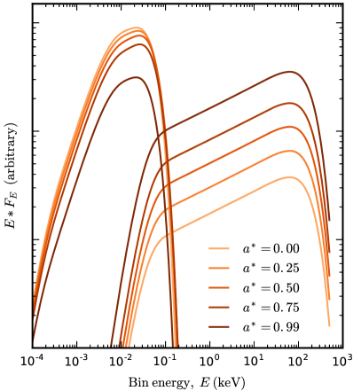
Changing the spin with the other parameters fixed has the effect of changing the relative flux contribution of the disk and non-thermal components. This effect is illustrated in Figure 1, which shows models with no intermediate component. As the spin of a SMBH increases, more energy is released by infalling matter; the additional energy is released close to the SMBH event horizon. When we fix the mass, coronal radius and luminosity, increasing the spin serves primarily to apportion more of the fixed luminosity to the part of the disk within the coronal radius, and hence to the non-thermal component. Hence has a similar effect to in that it changes the relative contributions of the disk and non-thermal components.
Figure 1 shows that the shape of the two spectral components is not strongly affected by (with . However the parameters and are not entirely degenerate in their effects on the spectral shape, since affects the spectral shape through modifying the radial functions , and in Equation 1, whereas determines which values of contribute to the disk emission.
The full and partial degeneracies discussed in the previous sections suggest that , , and could be combined into two parameters in a simplified model of the spectral shape - one parameter which shifts the disk emission in energy space, and one parameter which controls the relative flux between the disk and non-thermal components.
3. Shrinking the spectral model parameter space
We reduce the free parameter space of the optxagnf model by fixing or neglecting some parameters, and by reparametrizing the remaining parameter space.
3.1. Neglected or fixed parameters
3.1.1 Intermediate soft X-ray component
The origin of the widely-observed soft X-ray excess in AGN remains uncertain, despite recent progress. In particular, two general explanations are currently favored, which attempt to explain the relatively constant energy of the soft excess ( keV). These explanations are Comptonized disk emission (e.g. the treatment in optxagnf), and blurred reflection from the ionized accretion disk (e.g. Walton et al., 2013). Additionally, absorption has been seriously considered (e.g. Gierliński & Done, 2004), and there is evidence that a contribution to the soft X-ray excess comes from the wider NLR (e.g. Bianchi et al., 2006).
The possible physical processes that give rise to the centrally-originating soft excess may be constrained using hard and soft time lags (hard X-rays lagging soft X-rays and soft X-rays lagging hard X-rays) and correlations between spectral components. The time-delay of soft X-ray time lags is strongly correlated with black hole mass (De Marco et al., 2013).
Each soft X-ray excess photon with energy in the range keV will have less effect on the ionization state of the nebula than a photon with energy in the range keV. In the pilot study of Dopita et al. (2014) we found that the intermediate soft X-ray component was not required to achieve satisfactory fits to the optical emission-line spectrum of the Seyfert galaxy NGC 5427 with photoionization models, although the observed spectrum did not include high-ionization lines. We do however expect that the abundances of high ionization potential species such as Ar X (423 eV), Fe XIV (361 eV) and Fe X (234 eV) would be affected by dominant soft X-ray excesses. Additionally, a strong soft X-ray excess extends the partially-ionized zone, where Auger electrons produced by X-ray bombardment partially ionize the gas, and therefore must to some extent enhance emission of lines such as [O I] and [S II].
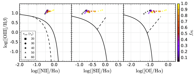
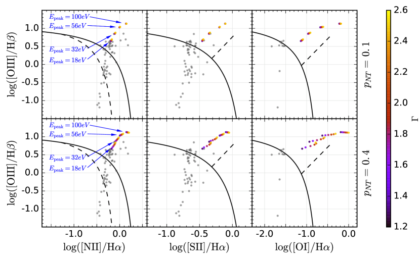
We performed an investigation on the effect of the soft excess on photoionization modeling of NLR clouds, using ionizing spectra from the optxagnf model. The parameters of the mappings 5.1111Available at http://miocene.anu.edu.au/Mappings (Sutherland et al. 2016, in prep.) models and optxangf spectra were fixed, apart from two quantities: the relative strength of the soft excess which ranged from to of the non-thermal flux, and the coronal radius which ranged from to . The models were ionization-bounded and ended when the nebula was 99% neutral. The results are presented in standard optical diagnostic diagrams (Baldwin, Phillips and Terlevich, 1981; Veilleux & Osterbrock, 1987) in Figure 2, with the fiducial model parameter values listed in the caption. The standard optical diagnostic diagrams use ratios of lines associated with different ionization levels in the gas to distinguish nebulae based on the cause of ionization. Ionization increases from bottom-left to top-right on the diagrams. The lower-left of each of the diagnostic diagrams is associated with H II regions of varying metallicity and ionization parameter, whereas the top-right is associated with ionization by harder AGN spectra or shocks. The standard dividing lines on the diagrams are described in the caption.
The results shown in Figure 2 confirm that the soft X-ray excess is not of primary importance when predicting diagnostic optical emission-line ratios. The line ratios are evidently most sensitive to variation in the coronal radius or weighting of spectral components when most of the energy released inside the coronal radius is emitted in the power-law component as opposed to the soft excess. For the tested values larger than 20 , the [S II]/H and [O I]/H ratios are significantly increased by increasing the proportion of the flux emitted in the power-law tail, resulting in some outlying points to the right of the second and third panel in the figure. The positions of these points are due to the partially-ionized zone being extended by hard X-rays in improbably hard ionizing spectra. If we do not consider these power-law dominated models (shown for completeness), the range of points representing the different soft excess strengths is small compared to the variation that may be produced by varying the ionization parameter or metallicity, for example. If the proportion of the energy emitted in the soft excess as opposed to the power-law component does not vary as strongly between real objects as it does in our experiment, and additionally if real objects are mass-bounded as opposed to ionization-bounded (i.e. hard X-rays escape the NLR), then the ranges shown in Figure 2 would represent approximate upper bounds on the sensitivity to the soft excess.
In the remainder of this work we do not include the intermediate Comptonized component, such that the fraction of the corona power in the power-law tail is set to , and the parameters for the temperature and optical thickness of the Comptonizing optically-thick medium have no effect.
Neglecting the intermediate component enables a vast simplification of the model. Including the soft excess would complicate the comparison of photoionization models to observed NLR emission-line spectra due to uncertainty regarding the origin, time-averaged behavior, and importance relative to other spectral components of the soft X-ray excess. We note that recently Pal et al. (2016) attributed of the keV emission observed in the AGN II Zw 177 to the soft excess, with significant variation observed between observations separated by 11 years. Another recent work is a study of the AGN RE J1034+396 (Czerny et al., 2016), in which the best-fitting models suggested that of the power produced inside the coronal radius is emitted in the intermediate component. Although the strength of the soft excess has been measured in sources such as II Zw 177 and RE J1034+396, the properties of the soft X-ray excess across the population of Seyfert galaxies, not just those that have been studied in X-rays, are unknown.
3.1.2 The black hole spin
The spins of astrophysical black holes have long been expected to be non-zero. It is now routine to ‘map’ the central of AGN accretion structures by studying X-ray reverberation lags and blurred accretion disk reflection (Fabian, 2016). Identifying the innermost radius required by spectral blurring analysis with the Innermost Stable Circular Orbit (ISCO) allows the black hole spin to be measured. Spin measurements performed to date generally demonstrate high spins (Reynolds, 2014). However because radiative efficiency increases by up to a factor of 5 with increasing spin, the very high calculated spins for many AGN with spin measurements are associated with a strong selection bias (Fabian, 2016).
As demonstrated above in Section 2.3, the black hole spin is partially degenerate with in that it changes the relative contributions of the disk and non-thermal components to the total spectrum. The coronal radius will be set larger than radii for which we expect the disk spectrum shape to be strongly affected by the SMBH spin. Figure 1 shows that changing the spin changes the relative energy in the disk and non-thermal components by an order of magnitude (between spins of 0 and 1); in our simplified model this effect will be accounted for by an explicit parameter for this scaling. The SMBH spin was set to .
3.1.3 Outer edge of accretion disk
The outer disk produces non-ionizing optical and IR emission, and therefore does not contribute to the NLR heating. The parameter defining the outer edge of the accretion disk was set to , a default value.
3.2. Reparametrizing the AGN continuum model
As a result of the simplifications discussed in the Section 3.1, the optxagnf parameters have been reduced to the four most important parameters , , and . Exploration of the properties of the theoretical AGN spectra and development of a simplified model (Section 4) were performed over the following ranges of these four parameters:
-
•
-
•
-
•
-
•
The maximum luminosity of Eddington was chosen because the Novikov-Thorne thin disk model cannot plausibly be used beyond this limit; indeed a slim disk prescription is necessary for a luminosity above . The range of SMBH masses covers the observed range in AGN except for extreme objects (c.f. Figure 4 in Vika et al. (2009)). The broad range in covers the approximate range of observed values (c.f. Figure 4 in Molina et al. (2013)), corresponding to very soft ( = 2.6) through to very hard ( = 1.4) power-law tails.
The physical extent of the corona has been constrained using analysis of blurred X-ray reflection, modeling of X-ray reverberation, and microlensing observations; these methods suggest that the Comptonizing corona lies within approximately of the black hole (Fabian, 2016). However because of the selection bias discussed in Section 3.1.2, coronal geometries inferred in X-ray studies are not necessarily representative of the population of Seyfert galaxies. We chose a lower bound for the coronal radius of 10 here; our experimentation showed that below this value the high-energy part of the accretion disk emission becomes too strongly affected by relativistic corrections for easy simplification of the model. Setting a minimum coronal radius of 10 will primarily affect the high-energy part of the accretion disk emission by removing it from the disk spectrum. The top end of the range was selected to include the range suggested by Done et al. (2012).
3.2.1 Reparametrizing the disk component
A highly desirable simplification is combining the three fully or partially degenerate parameters , and into a single parameter that is able to parametrize (at least approximately) the position in energy space and shape of the Big Blue Bump (BBB) disk emission. The parameter which was chosen to replace the degenerate trio (, , ) was , the peak of the BBB when the disk spectrum is given in a log-log plot of energy flux versus energy (e.g. Figure 1). The location of the single peak is a reliable and easily-calculated feature of a model BBB.
The value of was determined for a grid of optxagnf spectra over the relevant ranges of the three parameters affecting , which are , and . The results were systematically analyzed for each value of , before all the analyses for various values were combined into an empirical formula for calculating as a function of (, , ). An example of the analysis that was applied for a single value of is presented in Figure 3.
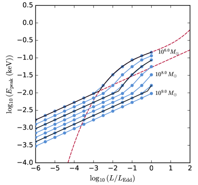
Figure 3 demonstrates how fits for at a given must account for the ‘piecewise’ behavior of as a function of and . Our solution to this problem was to use a combination of linear and cubic functions as described in the figure and caption. The coefficients of these linear and cubic functions varied as a function of . To construct a general function applicable over the entire three-dimensional (, , ) parameter space, we required a means to determine the coefficients of the linear and cubic functions from . Linear and quadratic functions of produced satisfactory fits to the values of these coefficients.
The analysis in Figure 3 was applied for , 10, 15, 24, 39, 63, 100 . The analysis for (i.e. at the innermost stable circular orbit, such that the corona is effectively absent) was found to be generally inconsistent with the analyses for the larger values, presumably due to the effect of strong general relativistic corrections. We thus did not use the analysis for .
The combined analysis for the various values culminated in the following equation for a hypersurface to predict as a function of , and :
| (4) |
where
| (5) |
and
| (6) |
Here the energy of the BBB peak is in keV, where is in M⊙, and . The fit parameters are given in Table 1. Note that and appear explicitly in Equations 5 and 6 only through the quantity , due to the complete degeneracy in their effects on the spectral shape (Section 2.1; note that there is an implicit dependence on in the normalization of and ). The arbitrary constant 6 occurs with in Equation 6 only because it was propagated through the analysis from the cubic functions such as those in Figure 3, where the cubic was fitted to the data (the lowest value we considered), and was shifted appropriately to apply to other values. Equations 4 to 6 in conjunction with Table 1 predict with a standard deviation of in linear energy space.
The shape of the BBB spectrum depends (to first order) only on the energies it covers, so we use to parametrize both the location in energy space and shape of the BBB emission. The construction of a simplified BBB model using this approach is discussed in Section 4.1.
3.2.2 Reparametrizing the non-thermal component
The shape of the non-thermal component is determined by the shape of the seed photon spectrum and by the parameter . The seed photon spectrum is a blackbody with a temperature which will be determined by the single parameter , so we have already reparametrized the shape of the non-thermal component such that it depends on only two parameters. The construction of the non-thermal emission component is discussed in Section 4.2.
4. The oxaf model
This section describes the construction of the oxaf model. In particular oxaf is a 3-parameter model, and the name oxaf, a contraction of optxagnf, was chosen to reflect that oxaf is in some sense a ‘reduced’ optxagnf.
The three parameters of the oxaf model are the energy of the peak of the Big Blue Bump (BBB) , the photon power-law index , and the proportion of the total energy flux emitted in the non-thermal component , with the remainder being in the BBB.
In optxagnf the shape of the BBB and the proportion of energy which goes to the power-law component are not independent, because both are affected by . However in oxaf, the parameters (which determines the BBB shape) and are independent by construction. For a given , oxaf does not have any parameters available to reproduce the variation in optxagnf BBB shapes which occurs as changes. However the variation of the BBB shape with is a small effect, so a single oxaf BBB is able to satisfactorily reproduce optxagnf BBBs which have the same peak energy but a range of (Section 4.4).
The following sections show how we construct a BBB using only one parameter, the energy of the BBB peak , and a non-thermal component using only two parameters ( and ).
4.1. Modeling the accretion disk emission
The BBB is parametrized using only one parameter, the energy of the BBB peak . The oxaf model must use this input to determine the shape of the BBB, in particular for relatively high BBB peak energies, when the color correction becomes important.
The modeled BBBs are considered in terms of log-log plots of energy flux (i.e. keV/cm2/s) versus energy. The effects of the color correction in this space are illustrated in Figure 4.
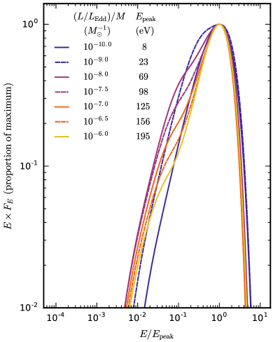
The oxaf model constructs the BBB as follows: sixth-order polynomials were fit to a series of optxangf BBBs at different energies ( = , , , , , ) roughly representative of the range of shapes shown in Figure 4. The BBBs were normalized to have the same peak flux and position of the peak flux in energy space before fitting. The coefficients of the fits are stored in the oxaf code. To determine the shape of an oxaf BBB for a given input , the code (log-)linearly interpolates between the polynomial fits for the nearest values above and below the input . The resulting polynomial BBB shape is a weighted sum of the two ‘nearest’ polynomials. The interpolated polynomial is shifted in energy space so the peak aligns with the input value.
4.2. Modeling the non-thermal emission
The non-thermal component is parametrized using two quantities: and .
The oxaf model uses the Nthcomp routine to generate an inverse-Compton scattered non-thermal component. The fortran subroutines donthcomp (Zdziarski et al., 1996; Życki et al., 1999), and thcompton with thermlc (Lightman & Zdziarski, 1987) from xspec were incorporated into oxaf.
There is one difference in the modeling of the non-thermal component between oxaf and optxagnf. In optxagnf the seed blackbody spectrum temperature is set to , the color-corrected temperature of the disc at . To approximate this method in oxaf it was necessary to convert the parameter to an estimate of , despite the oxaf model lacking an explicitly calculated . The conversion was achieved by extracting values for 72 representative optxagnf models across the parameter space and relating them to the values calculated for these models using Equation 4. The following linear fit from this comparison is used by oxaf to relate the two parameters:
| (7) |
where both and are measured in keV. Here the gradient and intercept have errors of 0.02 and 0.03 dex respectively, and the resulting error on is 0.07 dex. The non-thermal spectrum is constructed by converting to using Equation 7 before inputting , and an assumed Comptonizing plasma temperature of 100 keV into the oxaf donthcomp function, which in turn calls thcompton, which calls thermlc.
4.3. Implementation
The oxaf model was implemented as a module oxaf.py written in the programming language python, with a design focus on convenience of use. The module depends only on the standard third-party numerical Python library numpy, is a single file which may be used with both python 2 and python 3, and requires no compilation step to run (the included fortran codes were converted to python). The module may simply be run as a command line script to output a model spectrum to stdout, or alternatively may be imported to be used in python code. The module is thoroughly self-documented and is available on the Astrophysics Source Code Library (ASCL) 222Available at https://github.com/ADThomas-astro/oxaf (Not yet submitted to ASCL).
The oxaf.py module includes functions to find , the peak of the Big Blue Bump (BBB) disk emission (i.e. implement Equation 4), calculate an accretion disk spectrum (as described in Section 4.1), calculate a non-thermal component spectrum (as described in Section 4.2), and sum these two components using a given weighting.
The output spectrum is a function of only three parameters, being , , and , which is the proportion of the total flux over the range (keV) which is assigned to the non-thermal component, with being the proportion assigned to the BBB disk component.
The functions which return the individual components and the full spectrum (sum of the two components) normalize the spectra so that the sum of the bin fluxes over the range is equal to one.
4.4. Validation
The oxaf model was validated against the optxagnf model by comparing oxaf output with optxagnf output for many models across the parameter space. The BBB and non-thermal components were considered separately. The optxagnf parameters used were chosen so that their various combinations did not give multiple identical BBB peak energies and hence multiple identical oxaf spectra. The chosen values were = , -3.75, -2.85, -2.15, -1.60, -1.20, -0.80, -0.40, 0.00; = , 6.5, 7.0, 7.5, 8.0, 8.5, 9.0; = , 25, 40, 50, 63, 100 and = 1.4, 1.7, 2.0, 2.3, 2.6, for a total of 1890 optxagnf spectra. The range of parameters was chosen for completeness; not all of the tested parameter space necessarily corresponds to observed AGN.
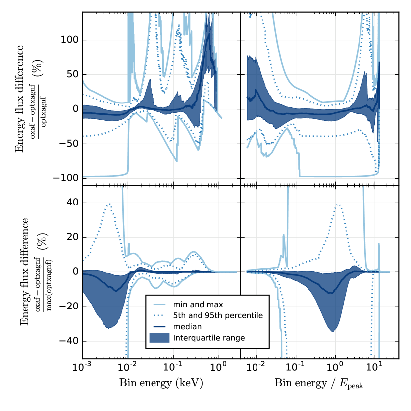
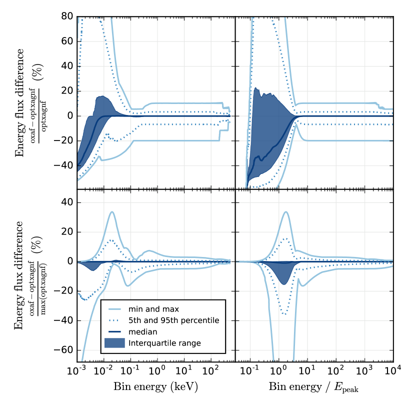
Figures 8 and 9 in the appendix demonstrate the performance of the oxaf model in reproducing the output spectra of optxagnf. The figures show that over the relevant energy range, from the Lyman limit to above the energy at which iron may be fully ionized (0.01 to 20 keV), oxaf predictions are sufficiently close to optxagnf predictions for our purposes (differences are far less than modeling uncertainties). The interquartile range displayed in each figure indicates that over the relevant energy range, oxaf predictions tend to be within 10-20% of the optxagnf value for the BBB component, and within for the non-thermal component. The largest deviations tend to occur for energies which are probably too high to have a strong impact on photoionization model results (1-10 keV) or are in an unlikely part of the parameter space (e.g. ). The most extreme discrepancies (i.e. 95th percentile and upwards) for the BBB comparisons tend to be due to irrelevant cases where only a small fraction of the total flux is in the relevant ionizing energy range, and hence the normalization over this range inflates a small section of the spectrum and magnifies proportional differences between the two models. For the non-thermal component the differences are due only to the small scatter in the fit given in Equation 7, i.e. the seed blackbody spectra for oxaf and optxagnf have slightly different temperatures.
The oxaf spectra reproduce the optxagnf models with sufficient accuracy for photoionization modeling of optical diagnostic emission lines. The differences between oxaf and optxagnf are smaller than the uncertainties due to, for example, any of the following:
-
•
The angular dependence of the accretion disk spectrum, including the effects of special relativistic beaming, gravitational beaming/light bending, and limb darkening (Laor & Netzer, 1989). Gravitational redshifts are an additional consideration.
-
•
Uncertainties in fundamental aspects of the thin disk model, such as the -prescription, and aspects of the geometry of the accretion disk and corona including the variation with black hole spin (e.g. You et al., 2012). The luminosity range over which the model is applicable is another consideration, e.g. for luminosities over a ‘slim’ disk is a more appropriate model.
-
•
Radiative transfer effects; for example, the use of a color correction in the optxagnf model neglects H and He edges (see Figure 1 in Done et al., 2012)
Two simple tests were performed to compare mappings 5.1 photoionization models based on optxagnf and oxaf spectra. For the first test the input optxagnf spectrum was configured with , , , , 2.2), while the oxaf spectrum was configured with , (68.3 eV, 2.2, 0.223), where was calculated from Equation 4 and was calculated to match the proportion in the optxagnf spectrum. The plane-parallel mappings models for this test were configured with a metallicity of , an ionization parameter of , and a constant pressure of K cm-3. The resulting line fluxes were broadly consistent between the two models. Of 43 optical lines with predicted fluxes of more than 1% of H, all had a flux discrepancy of less than 10% of the flux predicted using the optxagnf model. All but 4 line fluxes showed a difference of less than 5%; these 4 lines from N I or O I had differences of . The reason for this discrepancy is that these lines from low-ionization species are very sensitive to small differences in the shape of the hard photon spectrum since the emission is produced mostly in a partially ionized zone heated by Auger electrons.
For the second test the input optxagnf spectrum was configured with , , , , 1.8), while the oxaf spectrum was configured with , (19.9 eV, 1.8, 0.342). The mappings models used a metallicity of , an ionization parameter of , and a constant pressure of K cm-3. With the somewhat softer ionizing spectrum and different nebular parameters, there were only 31 optical lines with predicted fluxes of more than 1% of H, and all of those lines had a flux discrepancy below , with 24 having a discrepancy under .
The accuracy of oxaf is more than sufficient for our purposes of photoionization modeling.
5. The effect of oxaf parameters on predicted emission-line ratios
A grid of mappings photoionization models was used to explore the effect of the oxaf parameters on emission-line ratios on the standard optical diagnostic diagrams. The grid was run over a range of photoionization model parameters and a range of all three oxaf parameters. The results are shown in Figure 5 for the dusty, plane-parallel mappings models configured with metallicity , ionization parameter , and a constant pressure of K cm-3. Each model was iteratively re-run three times to ensure that the total pressure (including radiation pressure) was close to the input pressure, with this constraint applied where the model nebula was ionized. The iterations for each gridpoint culminated in a model which ended when the nebula was neutral.
Also plotted in Figure 5 are gray points showing the measured spatially-resolved line flux ratios for the galaxy NGC 1365 from the S7 galaxy survey (Dopita et al., 2015). Each point represents the line ratios for the narrowest Gaussian kinematic component in the spectrum of a 1”1” spatial pixel (the seeing FWHM was ”). A S/N cut of 10 was applied to the linear flux ratios. In the leftmost two columns of diagrams these points form a ‘mixing sequence’ from line-ratios associated with excitation purely due to star formation (at the bottom) to excitation purely by AGN radiation (at the top).
The predicted line ratios for our fiducial mappings models approximately coincide with some of the measured ‘pure-AGN’ line ratios, especially in the leftmost column. Predictions of the weaker [O I] line however are inconsistent with the observations. This line is produced predominantly in the partially ionized zone that arises due to the hard EUV and X-ray photons. The temperature and size of this region and thus the strength of the [O I] line are sensitive to the hard ionizing spectrum. In addition the fractional ionization state of oxygen is strongly dependent upon charge exchange reactions and as a result this line is very difficult to predict accurately. The [S II] 6716, 6731 doublet can also arise from this partially ionized region and is also somewhat inconsistent with the observations, albeit to a lesser degree. The overpredicted fluxes from these species could to some extent be due to the NLR clouds being mass-bounded as opposed to ionization-bounded (as in the models), i.e. more of the high-energy photons escape and the partially-ionized zones are shorter for the observed ensemble of NLR clouds in NGC 1365 compared to the models.
5.1. Effect of the individual oxaf parameters
In this section we discuss Figure 5 and interpret the effect of each oxaf parameter on the model predictions.
5.1.1 Energy of the peak of the disk emission
The logarithmically-spaced values of in Figure 5 show that increasing the energy of the peak of the disk emission, and thereby increasing the energy of the ionizing photons, increases both the relative ionization state and the temperature of the nebula. The sensitivity of optical diagnostic line ratios to is comparable to the sensitivity to the ionization parameter.
5.1.2 Proportion of flux in non-thermal component,
We first consider the expected range of values of . Jin et al. (2012a) study a sample of 51 unobscured Seyfert 1 galaxies and fit the full three-component optxagnf model to the observed SEDs. The proportion of the bolometric luminosity emitted in the power-law component in the best-fit model is less than 0.05 for of the sample, less than 0.2 for of the sample, and less than 0.4 for of the sample. Although the soft excess is a significant component (allocated more flux than the power-law component for of the sample), it is effectively an extension of accretion disk emission to higher energies, so the proportion of flux in the power-law tail is comparable to the oxaf parameter. Hence we take as an appropriate range for typical ionizing AGN spectra.
The values were included in the model grid but are not shown in Figure 5. The diagnostic line-ratio predictions for were intermediate between those of and and were similar to those of . The value was very high, with only a few extreme objects in the Jin et al. (2012a) sample having such power-law-dominated SEDs. Hence the figure requires only the values to indicate the effect of and show the approximate magnitude of strong line-ratio variations due to variations that may occur between Seyfert galaxies.
Increasing the value of increases the length of the trailing partially ionized zone in the photoionization models. For = 32 eV, = 1.8, U = -2.0 and Z = 1.5 Z⊙, variation of from 0.1 to 0.7 increased the length of the modeled cloud by a factor of to 1.5 pc. Extending the partially-ionized zone increases the [S II]/H and [O I]/H line ratios, as the figure shows for .
5.1.3 Photon index of the power-law tail
For values of , the predicted emission-line ratios do not show strong sensitivity to . Figure 5 shows how as increases, [S II] and [O I] line emission is enhanced relative to H. Increasing allocates more of the non-thermal energy to relatively soft X-ray photons which are more easily absorbed by the nebula, causing more emission in the partially ionized zone. Hence has a similar effect to . As increases, the sensitivity to increases due to the greater relative effect of X-ray power-law photons on the nebula ionization structure.
5.2. Comparison with default cloudy AGN spectrum
In this section we compare oxaf spectra with the default spectrum produced by the AGN spectral model supplied with the cloudy (Ferland et al., 2013) photoionization code. We also compare the predicted optical diagnostic emission-line ratios produced by using these ionizing spectra in MAPPINGS photoionization models.
The cloudy AGN spectral model uses an analytic formula consisting of exponential and power-law factors and terms. The default cloudy AGN model was configured with the following default values: a BBB temperature of K, an X-ray to UV ratio of , a low-energy BBB slope of , and an X-ray power-law index of (corresponding to ).
Figure 6 shows the cloudy default SED, along with two ‘equivalent’ oxaf spectra. The first oxaf spectrum has , (6.9 eV, 2.0, 0.46), chosen to match the BBB peak energy and the ‘height’ of the power-law tail, and has the same normalization as the normalized cloudy default SED. The second ‘equivalent’ oxaf spectrum has , (9.9 eV, 2.0, 0.414) to match the shape and position of the high-energy slope of the BBB and match the ‘height’ of the power-law tail. This second oxaf spectrum is shown with a different normalization, with only 73% of the energy flux of the cloudy spectrum, to show how it follows the shape of the cloudy spectrum in the important region associated with H-ionizing FUV photons.
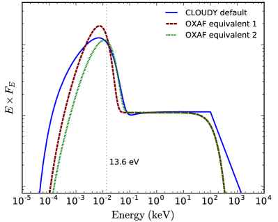
Clear differences between the spectral models are apparent in Figure 6. The cloudy model uses a single blackbody curve combined with a power-law to produce the BBB, resulting in a BBB much wider than the oxaf BBB. The physical model used to calculate the power-law tail in oxaf produces a power-law cutoff that is much steeper than the simple piecewise cutoff in the cloudy model.
Results of MAPPINGS photoionization model runs using the three spectra in Figure 6 are presented in Figure 7. The plane-parallel dusty MAPPINGS models were all configured with a metallicity of , an ionization parameter of , and a constant pressure of . All three models produced similar optical diagnostic line ratios. The second oxaf model resulted in line ratios closer to those due to the cloudy default spectrum, which confirms that the most important part of the spectrum for ionization modeling is the region immediately on the high-energy side of the H ionization threshold, where these spectra were very similar by design. The first oxaf model results in relatively lower [O III]H, which is presumably a consequence of the lower proportion of hydrogen-ionizing EUV photons.
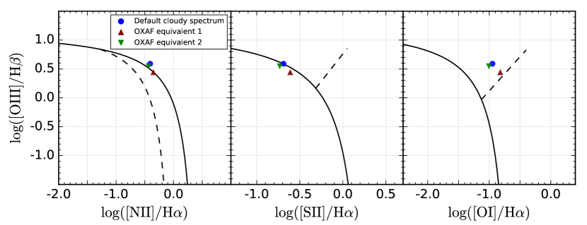
The results show that oxaf spectra may produce predicted diagnostic line ratios that are very similar to those resulting from analytic ionizing spectra not based on physical models, provided the spectral shapes are sufficiently well-matched in the most important part of the spectrum, the hydrogen-ionizing EUV.
6. Conclusions
We present a model of AGN continuum emission, oxaf, designed for use in photoionization modeling and featuring spectral shapes based on physical models. The oxaf model removes degeneracies between AGN parameters in terms of their effect on the ionizing spectral shape; in particular, in the thin disk accretion model the black hole mass and AGN luminosity are entirely degenerate with respect to their impact on the spectral shape. We base oxaf on the optxagnf model (Done et al., 2012), and explain and remove some additional spectral-shape degeneracies between AGN parameters when we reparametrize optxagnf.
We show that the soft X-ray excess is not important to photoionization modeling of the standard optical strong diagnostic lines, so we do not include it in the oxaf model. However the soft excess must be important in modeling forbidden high-ionization lines.
The model oxaf contains only three parameters - the energy of the peak of the accretion disk emission , the photon power-law index for the non-thermal Comptonized component , and the proportion of the total flux which goes to the non-thermal component . These parameters intuitively describe the physical shape of the produced spectrum.
We show that predicted ratios of strong lines on standard optical diagnostic diagrams are sensitive to all three oxaf parameters. The parameter directly affects the degree of ionization of the mappings model nebulae. The parameters and are similar in their effects in that they change the length of the partially-ionized zone. Predicted line-ratios are more sensitive to as is increased. Measured strong emission-line ratios for the Seyfert galaxy NGC 1365 are approximately consistent with the predictions of some fiducial photoionization models using input oxaf ionizing spectra.
Users of oxaf may further explore the effects of changing the shape of the ionizing spectrum on predicted emission-line spectra.
References
- Allen et al. (1998) Allen, M. G., Dopita, M. A., & Tsvetanov, Z. I. 1998, ApJ, 493, 571
- Antonucci (1993) Antonucci, R. 1993, ARA&A, 31, 473
- Baldwin, Phillips and Terlevich (1981) Baldwin, J. A., Phillips, M. M., & Terlevich, R. 1981, PASP, 93, 5
- Bianchi et al. (2006) Bianchi, S., Guainazzi, M., & Chiaberge, M. 2006, A&A, 448, 499
- Bland-Hawthorn et al. (2013) Bland-Hawthorn, J., Maloney, P. R., Sutherland, R. S., & Madsen, G. J. 2013, ApJ, 778, 58
- Collins et al. (2009) Collins, N. R., Kraemer, S. B., Crenshaw, D. M., Bruhweiler, F. C., & Meléndez, M. 2009, ApJ, 694, 765
- Contini & Viegas (2001) Contini, M., & Viegas, S. M. 2001, ApJS, 132, 211
- Czerny et al. (2016) Czerny, B., You, B., Kurcz, A., et al. 2016, arXiv:1601.02498
- Davies et al. (2016) Davies, R. L., Dopita, M. A., Kewley, L., et al. 2016, ApJ, 824, 50
- Davis et al. (2006) Davis, S. W., Done, C., & Blaes, O. M. 2006, ApJ, 647, 525
- Done et al. (2012) Done, C., Davis, S. W., Jin, C., Blaes, O., & Ward, M. 2012, MNRAS, 420, 1848
- De Marco et al. (2013) De Marco, B., Ponti, G., Cappi, M., et al. 2013, MNRAS, 431, 2441
- Dopita et al. (2002) Dopita, M. A., Groves, B. A., Sutherland, R. S., Binette, L., & Cecil, G. 2002, ApJ, 572, 753
- Dopita et al. (2014) Dopita, M. A., Scharwächter, J., Shastri, P., et al. 2014, A&A, 566, A41
- Dopita et al. (2015) Dopita, M. A., Shastri, P., Davies, R. L., et al. 2015, ApJS, 217, 12
- Evans et al. (1999) Evans, I., Koratkar, A., Allen, M., Dopita, M., & Tsvetanov, Z. 1999, ApJ, 521, 531
- Fabian (2016) Fabian, A. C. 2016, Astronomische Nachrichten, 337, 375
- Ferland et al. (2013) Ferland, G. J., Porter, R. L., van Hoof, P. A. M., et al. 2013, RMxAA, 49, 137
- Gierliński & Done (2004) Gierliński, M., & Done, C. 2004, MNRAS, 349, L7
- Groves et al. (2004) Groves, B. A., Dopita, M. A., & Sutherland, R. S. 2004, ApJS, 153, 9
- Groves et al. (2006) Groves, B. A., Heckman, T. M., & Kauffmann, G. 2006, MNRAS, 371, 1559
- Jin et al. (2012a) Jin, C., Ward, M., Done, C., & Gelbord, J. 2012, MNRAS, 420, 1825
- Jin et al. (2012b) Jin, C., Ward, M., & Done, C. 2012, MNRAS, 422, 3268
- Jin et al. (2012c) Jin, C., Ward, M., & Done, C. 2012, MNRAS, 425, 907
- Kauffmann et al. (2003) Kauffmann, G., Heckman, T. M., Tremonti, C., et al. 2003, MNRAS, 346, 1055
- Kewley et al. (2001) Kewley, L. J., Dopita, M. A., Sutherland, R. S., Heisler, C. A., & Trevena, J. 2001, ApJ, 556, 121
- Kewley et al. (2006) Kewley, L. J., Groves, B., Kauffmann, G., & Heckman, T. 2006, MNRAS, 372, 961
- Laor & Netzer (1989) Laor, A., & Netzer, H. 1989, MNRAS, 238, 897
- Lightman & Zdziarski (1987) Lightman, A. P., & Zdziarski, A. A. 1987, ApJ, 319, 643
- Molina et al. (2013) Molina, M., Bassani, L., Malizia, A., et al. 2013, MNRAS, 433, 1687
- Murayama & Taniguchi (1998) Murayama, T., & Taniguchi, Y. 1998, ApJ, 503, L115
- Novikov & Thorne (1973) Novikov, I. D., & Thorne, K. S. 1973, Black Holes (Les Astres Occlus), 343
- Page & Thorne (1974) Page, D. N., & Thorne, K. S. 1974, ApJ, 191, 499
- Pal et al. (2016) Pal, M., Dewangan, G. C., Misra, R., & Pawar, P. K. 2016, MNRAS, 457, 875
- Reynolds (2014) Reynolds, C. S. 2014, Space Sci. Rev., 183, 277
- Shakura & Sunyaev (1973) Shakura, N. I., & Sunyaev, R. A. 1973, A&A, 24, 337
- Veilleux & Osterbrock (1987) Veilleux, S., & Osterbrock, D. E. 1987, ApJS, 63, 295
- Viegas-Aldrovandi & Contini (1989) Viegas-Aldrovandi, S. M., & Contini, M. 1989, A&A, 215, 253
- Vika et al. (2009) Vika, M., Driver, S. P., Graham, A. W., & Liske, J. 2009, MNRAS, 400, 1451
- Walton et al. (2013) Walton, D. J., Nardini, E., Fabian, A. C., Gallo, L. C., & Reis, R. C. 2013, MNRAS, 428, 2901
- You et al. (2012) You, B., Cao, X., & Yuan, Y.-F. 2012, ApJ, 761, 109
- Zdziarski et al. (1996) Zdziarski, A. A., Johnson, W. N., & Magdziarz, P. 1996, MNRAS, 283, 193
- Życki et al. (1999) Życki, P. T., Done, C., & Smith, D. A. 1999, MNRAS, 309, 561