NLO predictions for SMEFT in the top-quark sector

Abstract:

Predictions for the Standard Model Effective Field Theory at the next-to-leading order accuracy in QCD, including parton-shower effects, have started to become available in the MadGraph5_aMC@NLO framework. In this talk we summarize some recent results for $t\bar{t}$, single top, $t\bar{t}Z/\gamma$, and $t\bar{t}H$ production channels at dimension six.

1 Introduction

The Standard Model Effective Field Theory (SMEFT) at dimension-six [1] is a powerful approach to the SM deviations. By supplementing the SM Lagrangian with a set of higher-dimensional operators, indirect effects from heavy particles, possibly beyond the reach of the LHC, can be consistently accommodated. Given that the expectations from LHC Run-II on the attainable precision of the top-quark measurements are very high, next-to-leading order (NLO) predictions for top-quark production channels are becoming relevant, not only for the SM background but also for the deviations from dimension-six operators, mainly for the following reasons:

• At the LHC, the impact of QCD corrections on total cross sections are often large, which might improve the exclusion limits on effective operators. In addition, NLO corrections reduce the theoretical uncertainties due to missing higher-order corrections. This helps to discriminate between different new physics scenarios.

• QCD corrections often change the distributions of key observables. As differential distributions start to play an important role in recent global analyses based on SMEFT, reliable predictions for the distributions are needed. In section 3 we will show an example where this effect is crucial.

• Sensitivity to effective deviations can be improved by making use of the accurate SMEFT predictions and designing optimized experimental strategies in a top-down way. However, given the large QCD corrections at the LHC, this improvement will be difficult without consistent SMEFT at NLO predictions.

Recently, NLO predictions for the SMEFT, matched with parton shower simulation, are becoming available in the MadGraph5_aMC@NLO framework [2], based on an automatic approach to NLO QCD calculation interfaced with shower via the MC@NLO method [3]. The dimension-six Lagrangian can be implemented with the help of a series of packages, including FeynRules and NLOCT [4, 5, 6, 7, 8, 9]. A model in the Universal FeynRules Output format [6] can be built, allowing for simulating a variety of processes at NLO in QCD. In this talk we summarize some recent progresses in this direction, with a focus on the top-quark sector. The interested readers may find more details in Refs. [10, 11, 12, 13].

2 Top-pair production

The chromo-dipole operator for the top quark, $O_{tG}=g_{s}y_{t}\left(\bar{Q}\sigma^{\mu\nu}T^{A}t\right)\tilde{\phi}G^{A}_{\mu\nu}$, can be constrained by top-pair production. Here $g_{s}$ is the strong interaction coupling, and $y_{t}$ is the top Yukawa coupling. $Q$ is the third generation left-handed quark doublet, while $t$ is the right-handed top quark. Assuming real operator coefficient, this calculation has been carried out at NLO in Ref. [10]. In Figure 1 we present the invariant mass distribution at LHC 8 TeV. The $K$-factors for the total cross sections are found to be $1.1$, $1.4$, and $1.5$ respectively for Tevatron, LHC 8 TeV, and LHC 13/14 TeV. As a result, the current limits on the chromomagnetic dipole moment of the top quark from direct measurements can be improved by roughly the same factors. In Table 1 we compare the limits on $C_{tG}/\Lambda^{2}$ at LO and at NLO.

Figure 1: Top quark pair invariant mass distribution at LHC 8 TeV.

	LO [TeV-2]	NLO [TeV-2]
Tevatron	[-0.33, 0.75]	[-0.32, 0.73]
LHC8	[-0.56, 0.41]	[-0.42, 0.30]
LHC14	[-0.56, 0.61]	[-0.39, 0.43]

Table 1: Limits on $C_{tG}/\Lambda^{2}$. The corresponding limits combining Tevatrion and LHC8, in terms of $d_{V}$, is $[-0.0099,0.0123]$ at LO and $[-0.0096,0.0090]$ at NLO. For LHC14 we assume a $5\%$ experimental error.

3 Single top production

Single top production has been computed in all three channels ($t$-channel, $s$-channel, and $tW$ associated production channel) at NLO in QCD, with the following operators:

$$O_{\phi Q}^{(3)}=i\frac{1}{2}y_{t}^{2}\left(\phi^{\dagger}\overleftrightarrow{D}^{I}_{\mu}\phi\right)(\bar{Q}\gamma^{\mu}\tau^{I}Q)\;,\qquad O_{tW}=y_{t}g_{W}(\bar{Q}\sigma^{\mu\nu}\tau^{I}t)\tilde{\phi}W_{\mu\nu}^{I}\;,$$ (1)

$$O_{qQ,rs}^{(3)}=(\bar{q}_{r}\gamma_{\mu}\tau^{I}q_{s})(\bar{Q}\gamma^{\mu}\tau^{I}Q)\;,$$ (2)

and $O_{tG}$ [11]. Here $q_{r}$ and $q_{s}$ are the quark doublet fields in the first two generations. $r,s$ are flavor indices. $g_{W}$ is the SM weak coupling constant. The operators $O_{tG}$ and $O_{tW}$ have mixing effect. Total cross sections (including top and antitop) at LHC 13 TeV are presented in Figure 3. The ratios between the interference cross sections, $\sigma^{(1)}_{i}$, and the SM NLO cross section, $r_{i}=\left|\sigma^{(1)}_{i}\right|/\sigma_{\mathrm{SM}}^{\mathrm{NLO}}$, for individual operators $O_{i}$, are given in all three channels. Scale uncertainties from the numerator are given, and in the lower panel the $K$-factor of each operator contribution is shown. Improved accuracy is reflected by the $K$-factors, typically ranging from $\sim 10\%$ to $\sim 50\%$, and improved precision is reflected by the significantly reduced scale uncertainties.

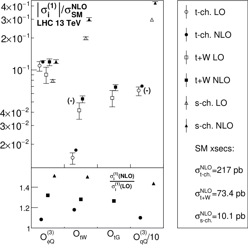
Figure 2: $r_{i}=\left|\sigma^{(1)}_{i}\right|/\sigma_{\mathrm{SM}}^{\mathrm{NLO}}$ for the three single-top channels. Both LO and NLO results are shown. Error bars indicate scale uncertainties. $K$-factors are given in the lower panel. Negative contributions are labeled with “(-)”.

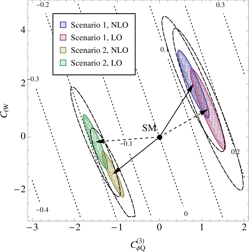
Figure 3: Two-operator fit using single-top pseudomeasurements on shapes, at 68% confidence level, assuming 5% uncertainty in each bin. Dashed lines correspond to twice this uncertainty, while dotted contours are the relative deviation in total cross section.

QCD corrections to the shapes of discriminator observables could lead to bias in an SMEFT analysis, by shifting the theoretical predictions for the shapes of the observables. This effect might lead to a different direction in which new physics deviates from the SM. As a result, if deviations due to new physics are observed, missing QCD corrections could lead us to misinterpret the measurements and misconclude the nature of UV physics. An example of a two-operator fit using pseudomeasurements in $t$-channel single top is given in Figure 3, assuming two scenarios: $(C_{\phi Q}^{(3)},C_{tW})=(0.8,2.0)$, and $(C_{\phi Q}^{(3)},C_{tW})=(-1.1,-1.4)$. More details can be found in Ref. [11].

4 Top-pair production in association with a gauge boson

At the LHC, the neutral couplings $ttZ$ and $tt\gamma$ can be probed by associated production of a top-quark pair with a neutral gauge boson $Z/\gamma$. The relevant operators, apart from $O_{tG}$, $O_{\phi Q}^{(3)}$, and $O_{tW}$, are:

$$O_{\phi Q}^{(1)}=i\frac{1}{2}y_{t}^{2}\left(\phi^{\dagger}\overleftrightarrow{D}_{\mu}\phi\right)(\bar{Q}\gamma^{\mu}Q)\;,\qquad O_{\phi t}=i\frac{1}{2}y_{t}^{2}\left(\phi^{\dagger}\overleftrightarrow{D}_{\mu}\phi\right)(\bar{t}\gamma^{\mu}t)\;,$$ (3)

$$O_{tB}=y_{t}g_{Y}(\bar{Q}\sigma^{\mu\nu}t)\tilde{\phi}B_{\mu\nu}\;.$$ (4)

The corresponding NLO predictions are given in Ref. [12]. Here we only present a summary plot for total cross sections in Figure 4, similar to Figure 3. By studying the differential distributions, we also find that the differential $K$-factor of the SM and that of the operator contribution can be quite different, therefore using the SM $K$-factor to rescale the operator contributions may not be a good approximation. Finally, $e^{+}e^{-}\to t\bar{t}$ with the same operators have also been computed.

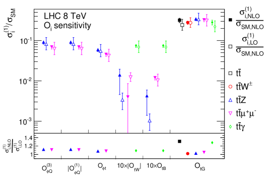
Figure 4: Sensitivity of various top quark processes to the various operators shown at LO and NLO at 8 TeV. $K$-factors are also shown for $\sigma^{(1)}_{i}$ as well as the scale uncertainties. We do not show the $K$-factors for the $O_{tB}$ and $O_{tW}$ operators in the $t\bar{t}Z$ and $t\bar{t}\mu^{+}\mu^{-}$ processes, as there are accidental cancellations that lead to large or even negative $K$-factors.

5 Top-pair production in association with a Higgs boson

The LHC provides us the first chance to directly measure the interactions between the top quark and the Higgs boson through the associated production of a Higgs with $t\bar{t}$. In Ref. [13], this process has been computed at NLO including three operators: the chromo-dipole operator $O_{tG}$, the Yukawa operator $O_{t\phi}=y_{t}^{3}\left(\phi^{\dagger}\phi\right)\left(\bar{Q}t\right)\tilde{\phi}$, and the Higgs-gluon operator $O_{\phi G}=y_{t}^{2}\left(\phi^{\dagger}\phi\right)G_{\mu\nu}^{A}G^{A\mu\nu}$. The QCD mixing of these three operators goes in the direction of increasing number of Higgs fields, i.e. $O_{tG}$ mixes into $O_{\phi G}$, and both of them mix into $O_{t\phi}$, but not the other way around.

Cross sections from dimension-six operators can be parametrized as

$$\sigma=\sigma_{SM}+\sum_{i}\frac{1{\rm TeV}^{2}}{\Lambda^{2}}C_{i}\sigma_{i}+\sum_{i\leq j}\frac{1{\rm TeV}^{4}}{\Lambda^{4}}C_{i}C_{j}\sigma_{ij}.$$ (5)

As an example we present here $\sigma_{i}$ and $\sigma_{ij}$ in Table 2. For each central value we quote three uncertainties. The first is the standard scale uncertainty from renormalization and factorization scales. The third uncertainty comes from the PDF sets. The second one is new in the SMEFT. It comes from the EFT scale uncertainty, representing the missing higher-order corrections to the operators. A more detailed discussion can be found in Ref. [13].

	$\sigma$ NLO	$K$
$\sigma_{SM}$	$0.507^{+0.030+0.000+0.007}_{-0.048-0.000-0.008}$	1.09
$\sigma_{t\phi}$	$-0.062^{+0.006+0.001+0.001}_{-0.004-0.001-0.001}$	1.13
$\sigma_{\phi G}$	$0.872^{+0.131+0.037+0.013}_{-0.123-0.035-0.016}$	1.39
$\sigma_{tG}$	$0.503^{+0.025+0.001+0.007}_{-0.046-0.003-0.008}$	1.07
$\sigma_{t\phi,t\phi}$	$0.0019^{+0.0001+0.0001+0.0000}_{-0.0002-0.0000-0.0000}$	1.17
$\sigma_{\phi G,\phi G}$	$1.021^{+0.204+0.096+0.024}_{-0.178-0.085-0.029}$	1.58
$\sigma_{tG,tG}$	$0.674^{+0.036+0.004+0.016}_{-0.067-0.007-0.019}$	1.04
$\sigma_{t\phi,\phi G}$	$-0.053^{+0.008+0.003+0.001}_{-0.008-0.004-0.001}$	1.42
$\sigma_{t\phi,tG}$	$-0.031^{+0.003+0.000+0.000}_{-0.002-0.000-0.000}$	1.10
$\sigma_{\phi G,tG}$	$0.859^{+0.127+0.021+0.017}_{-0.126-0.020-0.022}$	1.37

Table 2: NLO cross sections in pb for $pp\to t\bar{t}H$ at 13 TeV, and corresponding $K$-factors.

Figure 5: Comparison of the RG corrections with the exact NLO results for $t\bar{t}H$ production.

It is also interesting to compare the two kinds of corrections, i.e. RG and full NLO, in the $t\bar{t}H$ process. In Figure 5 we show the interference cross sections from three operators calculated as functions of $\mu_{EFT}$ for $\Lambda=2$ TeV, where LO contributions are normalized at 2 TeV. The dashed lines indicate corrections from one-loop RG only, ranging from roughly $0$ to $40\%$. Full NLO gives much larger corrections as indicated by the solid lines. This plot clearly demonstrates that RG corrections are far from a good approximation to NLO corrections.

6 Summary

We have briefly discussed several recent works on NLO predictions for SMEFT in the top-quark sector. These studies pave the way towards an accurate global fit for top-quark interactions.

- [1] W. Buchmuller and D. Wyler, Effective Lagrangian Analysis of New Interactions and Flavor Conservation, Nucl. Phys. B 268, 621 (1986).
- [2] J. Alwall et al., The automated computation of tree-level and next-to-leading order differential cross sections, and their matching to parton shower simulations, JHEP 1407, 079 (2014) [arXiv:1405.0301 [hep-ph]].
- [3] S. Frixione and B. R. Webber, Matching NLO QCD computations and parton shower simulations, JHEP 0206, 029 (2002) [hep-ph/0204244].
- [4] A. Alloul, N. D. Christensen, C. Degrande, C. Duhr and B. Fuks, FeynRules 2.0 - A complete toolbox for tree-level phenomenology, Comput. Phys. Commun. 185, 2250 (2014) [arXiv:1310.1921 [hep-ph]].
- [5] C. Degrande, Automatic evaluation of UV and R2 terms for beyond the Standard Model Lagrangians: a proof-of-principle, Comput. Phys. Commun. 197, 239 (2015) [arXiv:1406.3030 [hep-ph]].
- [6] C. Degrande, C. Duhr, B. Fuks, D. Grellscheid, O. Mattelaer and T. Reiter, UFO - The Universal FeynRules Output, Comput. Phys. Commun. 183, 1201 (2012) [arXiv:1108.2040 [hep-ph]].
- [7] P. de Aquino, W. Link, F. Maltoni, O. Mattelaer and T. Stelzer, ALOHA: Automatic Libraries Of Helicity Amplitudes for Feynman Diagram Computations, Comput. Phys. Commun. 183, 2254 (2012) [arXiv:1108.2041 [hep-ph]].
- [8] V. Hirschi, R. Frederix, S. Frixione, M. V. Garzelli, F. Maltoni and R. Pittau, Automation of one-loop QCD corrections, JHEP 1105, 044 (2011) [arXiv:1103.0621 [hep-ph]].
- [9] R. Frederix, S. Frixione, F. Maltoni and T. Stelzer, Automation of next-to-leading order computations in QCD: The FKS subtraction, JHEP 0910, 003 (2009) [arXiv:0908.4272 [hep-ph]].
- [10] D. Buarque Franzosi and C. Zhang, Probing the top-quark chromomagnetic dipole moment at next-to-leading order in QCD, Phys. Rev. D 91, no. 11, 114010 (2015) [arXiv:1503.08841 [hep-ph]].
- [11] C. Zhang, Single Top Production at Next-to-Leading Order in the Standard Model Effective Field Theory, Phys. Rev. Lett. 116, no. 16, 162002 (2016) [arXiv:1601.06163 [hep-ph]].
- [12] O. Bessidskaia Bylund, F. Maltoni, I. Tsinikos, E. Vryonidou and C. Zhang, Probing top quark neutral couplings in the Standard Model Effective Field Theory at NLO in QCD, JHEP 1605, 052 (2016) [arXiv:1601.08193 [hep-ph]].
- [13] F. Maltoni, E. Vryonidou and C. Zhang, Higgs production in association with a top-antitop pair in the Standard Model Effective Field Theory at NLO in QCD, JHEP 1610, 123 (2016) [arXiv:1607.05330 [hep-ph]].