Small-scale galaxy clustering in the eagle simulation

Abstract

We study present-day galaxy clustering in the eagle cosmological hydrodynamical simulation. eagle’s galaxy formation parameters were calibrated to reproduce the redshift $z=0.1$ galaxy stellar mass function, and the simulation also reproduces galaxy colours well. The simulation volume is too small to correctly sample large-scale fluctuations and we therefore concentrate on scales smaller than a few mega parsecs. We find very good agreement with observed clustering measurements from the Galaxy And Mass Assembly (gama) survey, when galaxies are binned by stellar mass, colour, or luminosity. However, low-mass red-galaxies are clustered too strongly, which is at least partly due to limited numerical resolution. Apart from this limitation, we conclude that eagle galaxies inhabit similar dark matter haloes as observed gama galaxies, and that the radial distribution of satellite galaxies as function of stellar mass and colour is similar to that observed as well.

1 Introduction

The spatial distribution of galaxies provides a powerful way to probe both cosmology and galaxy formation. Galaxy clustering measurements on scales where density fluctuations are only mildly non-linear, combined with other cosmological data sets such as CMB measurements, put impressively tight constraints on cosmological parameters (e.g. Hinshaw et al., 2013; Planck Collaboration et al., 2016). In addition, the detection of baryon acoustic oscillations in the clustering of galaxies (e.g. Cole et al., 2005; Eisenstein et al., 2005) opened up the way to quantify the nature of dark energy (e.g. Laureijs et al., 2011), and combined with redshift-space distortion measurements, test theories of gravity (e.g. Linder, 2008).

From the perspective of galaxy formation, the clustering of galaxies inform us about the relation between galaxies and the underlying dark matter and can provide hints about the physical processes involved in galaxy assembly history. As galaxies reside within the dark matter haloes, their positions trace the underlying cosmic structure. While the formation and evolution of the dark matter haloes is governed exclusively by gravitational interaction, the assembly of the galaxies is governed by the more complex baryon physics that also affects the distribution of galaxies. Such ‘galaxy bias’ may impact as well cosmological inferences made from galaxy clustering measurements.

The main statistical tool used for characterising galaxy clustering is the two-point correlation function $\xi$(r), which measures the excess probability over random of finding pairs of galaxies at different separations $r$ (Peebles, 1980). Commonly, when analysing redshift surveys, the projected correlation function integrated along the line-of-sight is used, in order to eliminate in principle redshift-space distortions (Davis & Peebles, 1983). Observations show that brighter, redder and more massive galaxies are more strongly clustered and related trends are also measured as a function of morphology and spectral type (e.g., Norberg et al. 2002a; Zehavi et al. 2002, 2005; Goto et al. 2003; Li et al. 2006; Coil et al. 2006; Croton et al. 2007; Zheng et al. 2007; Coil et al. 2008; Zehavi et al. 2011; Coupon et al. 2012; Guo et al. 2013; Farrow et al. 2015).

The theoretical modelling of galaxies plays an important role in interpreting clustering data, since, although galaxy clustering on large enough scales is very similar to that of the underlying matter distribution, it is not expected to be identical. Such models are also routinely used to estimate sample variance and verify methods for correcting observational biases. Several theoretical schemes are able to model galaxy clustering in volumes comparable to those probed observationally. These start from a dark matter only (DMO) $N$-body simulation, and populate haloes or sub-haloes with galaxies. Halo occupation distribution models (hod, e.g. Cooray, 2002; Berlind & Weinberg, 2002; Tinker et al., 2012) or sub-halo abundance matching (sham, e.g. Conroy et al., 2006; Vale & Ostriker, 2004, 2006) are statistical techniques that match galaxies with haloes by abundance based on, for example, their circular velocity. Semi-analytical galaxy formation techniques (e.g. Kauffmann et al., 1993; Cole et al., 1994) use physically motivated schemes to associate galaxies to haloes (see e.g. Baugh, 2006, for a review).

Notwithstanding the successes of these methods, they suffer from intrinsic limitations. Stellar and AGN feedback from forming galaxies affect the mass of their halo (Sawala et al., 2013; Velliscig et al., 2014; Schaller et al., 2015), limiting the extent to which any DMO simulation predicts the clustering of haloes as function of mass accurately. Feedback effects are plausibly strong enough to affect the mass distribution itself (van Daalen et al., 2011; Semboloni et al., 2011) and with it galaxy clustering (Hellwing et al., 2016). These effects may be relatively small, but the main limitation of the models is on smaller scales, where several effects that occur when a galaxy becomes a satellite (tidal interactions, ram-pressure stripping, strangulation) come into play. van Daalen et al. (2014) investigate how physics behind galaxy formation affect the clustering of galaxies at small scales through comparing two models of owls project (Schaye et al., 2010) with and without AGN feedback. They found that the physics of galaxy formation affects clustering on small scales, and in addition affects larger scales through its impact on the masses of sub halos. Farrow et al. (2015) show how clustering in galaxy light cone mocks generated with two versions of the semi-analytical galform code (Lacey et al., 2016; Gonzalez-Perez et al., 2014) differ significantly with the observations on small scales. McCullagh et al. (in prep.) and Gonzalez-Perez et al. (2017) show that once a more detailed merger scheme is considered, such as that described by Simha & Cole (2013) reasonably good agreement with clustering data on small scale is achieved. This is in agreement with the findings of Contreras et al. (2013) in which different families of galaxy formation models were compared to clustering data. McCarthy et al. (2016) present results from the bahamas cosmological hydrodynamical simulation. These simulations were designed using a similar calibration strategy as eagle but using the owls implementation of galaxy formation described by Schaye et al. (2010). The simulated volume (400 Mpc/$h$ on a side) and mass resolution (initial baryonic particle mass $8\times 10^{8}h^{-1}{\rm M}_{\odot}$) allow them to probe the galaxy correlation function on large scales, but not to go to lower-mass galaxies and smaller scale clustering that we concentrate on here, nor to investigate clustering as function of galaxy property such as for example colour. Sales et al. (2015) compare the distribution of satellite galaxies from the illustris simulation (Vogelsberger et al., 2014) as function of colour to Sloan Digital Sky Survey (sdss, York et al. 2000) observations by Wang et al. (2014). They attribute the better agreement of the simulations compared to semi-analytical models to the more realistic gas contents of satellites at infall.

Galaxy clustering on small scales, and as a function of intrinsic galaxy properties such as luminosity, colour and star formation rate, thus might prove to be a stringent test of galaxy formation models. Performing such a test is the aim of this paper: we explore the clustering of galaxies in the cosmological hydrodynamical eagle simulation (Schaye et al., 2015) and its dependence on galaxy properties. The galaxy formation model of eagle uses sub-grid modules that are calibrated to reproduce the present-day stellar mass function (as described by Crain et al., 2015). In addition, the eagle simulation reproduces relatively well the colours and luminosities of galaxies both in the infra-red (Camps et al., 2016) and at optical wavelengths (Trayford et al., 2016).

The 100 Mpc extent of the largest eagle simulation volume analysed in this paper is too small to properly sample large-scale modes, and, as is well known, such missing large-scale power quantitatively affects clustering measures even on smaller scales (e.g. Bagla & Ray, 2005; Bagla & Prasad, 2006; Trenti & Stiavelli, 2008). To estimate the severity of this, we compare the clustering of haloes in a dark matter- only version of the eagle volume to that in a much larger volume, simulated with the same cosmological parameters. This allows us to estimate the limitations of our approach. We compare the eagle predictions to clustering measurements by Farrow et al. (2015) of galaxies in the Galaxy and Mass Assembly redshift survey (gama, Driver et al., 2011; Liske et al., 2015), which are in accord with the Zehavi et al. (2011) sdss measurements. For completeness we note that Crain et al. (2016) show that eagle reproduces the observed clustering of $z=0$ Hi sources.

This paper is organised as follows. In  § 2 we describe the main characteristics of the simulations used, and briefly discuss the gama survey to which we compare. In  § 3 we define the notation and present the tools used to measure galaxy clustering. Simulations and observations are compared in  § 4. In the discussion section, § 5, we compare eagle with the clustering in galform (following the analysis of Farrow et al., 2015) and our own clustering measurements using the database of the illustris (Vogelsberger et al., 2014) simulation. The conclusions are summarised in  § 6.

Throughout this paper and unless specified otherwise, we use the Planck Collaboration et al. (2014) values of the cosmological parameters ($\Omega_{\rm b}=0.0482$, $\Omega_{\rm dark}=0.2588$, $\Omega_{\Lambda}=0.693$ and $h=0.6777$, where $H_{0}=100\;h$ km s^-1 Mpc^-1. Observational measures of clustering are (most commonly) specified in ‘$h$’-dependent units, and to ease comparison to other clustering studies, we will express distances in $h^{-1}$ Mpc and masses in $h^{-2}$M_⊙.

2 Simulations and Data

This section briefly describes the simulations used, and the gama survey to which clustering results of the simulations are compared.

Table 1: Numerical parameters of cosmological simulations considered. From left to right: simulation identifier, simulation co-moving side length $L$, initial mass $m_{\rm g}$ of baryonic particles, dark matter particle mass, Plummer-equivalent co-moving length ($\epsilon_{\rm com}$) and maximum proper gravitational softening length $\epsilon_{\rm prop}$. The eagle and eagle-dmo simulations are referred to as L0100N1504 and L0100N1504-DMO by Schaye et al. (2015).

Name	$L$	$m_{\rm g}$	$m_{\rm dm}$	$\epsilon_{\rm com}$	$\epsilon_{\rm prop}$
	$h^{-1}$Mpc	$10^{6}\,{\rm M}_{\odot}$	$10^{6}\,{\rm M}_{\odot}$	kpc	kpc
eagle	67.77	1.81	9.70	2.66	0.7
eagle-dmo	67.77	-	11.51	2.66	0.7
p-millennium	542.16	-	157	3.40	3.40

2.1 The eagle hydrodynamical simulation suite

Figure 1: Distribution of rest-frame $(g-r)_{0}$ colour versus $r$-band absolute magnitude, for $z=0.1$ eagle galaxies (coloured points). The rapid colour-dependent decline of galaxies fainter than $M_{\rm r}-5\log_{10}(h)=-17$ results from imposing a stellar mass cut of $M_{*}>10^{8.66}h^{-2}M_{\odot}$. The solid black line from Eq. (2) distinguishes red from blue galaxies, eagle galaxies above (below) this line line are represented by a red (blue) dot. The black dashed-line is the corresponding colour-cut from Farrow et al. (2015) for gama galaxies (their Eq. 4, and Eq. 1 in the text)

We use the ‘reference’ eagle simulation from Table 2 in Schaye et al. (2015) (i.e. L0100N1504, but hereafter referred to as the eagle simulation), a hydrodynamical cosmological simulation that start at $z=127$ from initial conditions generated using the panphasia multi-resolution phases of Jenkins & Booth (2013), taking the Planck Collaboration et al. (2014) cosmological parameter values. The simulation is part of the eagle simulation suite (Schaye et al., 2015; Crain et al., 2015) and Table 1 lists some of the key simulation parameters. The eagle simulations were performed with the gadget-3 code, which is based on gadget-2 (Springel, 2005), and uses ‘sub grid models’, briefly discussed in more detail below, to encode physical processes below the resolution limit. These models are formulated using parameters or functional forms that express limitations in our understanding of a given process (for example star formation) or our inability to simulate accurately a known process because of lack of numerical resolution (e.g. the effect of a supernova explosion on the interstellar medium in the presence of radiative cooling). These parameters and functions are calibrated so that the simulation reproduces a limited set of observed properties of galaxies, by performing a large set of simulations in which these parameters are varied as described by Crain et al. (2015). The set of constraints is limited, mainly because each simulation takes a long time to run. In the case of eagle, sub grid parameters were calibrated to observations at $z\approx 0$ of the galaxy stellar mass function of Baldry et al. (2012), galaxy sizes as measured by Shen et al. (2003), and the relation between black hole mass and stellar mass.

The hydrodynamics used in eagle uses a number of improvements to the SPH implementation collectively referred to as anarchy and described by Dalla Vecchia (in prep.); see Schaller et al. (2015) for a discussion of the relatively small impact of these changes on the properties of simulated galaxies. We briefly summarise below the sub grid modules for unresolved physics relevant for this paper:

• Photo-heating and radiative cooling by the optically thin evolving UV/X-ray background of Haardt & Madau (2001) is implemented element-by-element as described by Wiersma et al. (2009a).

• Star formation is implemented using the pressure law of Schaye & Dalla Vecchia (2008) and the metallicity-dependent star formation threshold of Schaye (2004). Gas particles eligible for star formation are converted to ‘star particles’ stochastically with a probability that depends on their star formation rate and their time step.

• Stellar evolution and enrichment is implemented as described by Wiersma et al. (2009b): assuming stars form with the Chabrier (2003) stellar initial mass function (IMF), spanning the range [0,1,100] M_⊙, we use stellar evolution and yield tables to calculate the rate of type Ia and type II (core-collapse) supernovae, and follow the rate at which stars enrich the interstellar medium through AGB, type Ia and type II evolutionary channels.

• Seeding, accretion and merging of black holes is implemented following Springel et al. (2005); Booth & Schaye (2009), modified to account for the angular momentum of accreted gas as described by Rosas-Guevara et al. (2015).

• Thermal feedback from stars is implemented as described by Dalla Vecchia & Schaye (2012); feedback from accreting black holes is also implemented thermally.

• Dark matter haloes are identified using the friends-of-friends algorithm, with baryonic particles (gas, stars, and black holes) assigned to the same halo as the nearest dark matter particle, if any. The mass of the halo is characterised by $M_{h}\equiv M_{200,c}$, the mass enclosed within a sphere within which the mean density is 200 times the critical density.

• Galaxies are identified using the subfind algorithm (Springel et al., 2001; Dolag et al., 2009). To avoid including ‘intra-cluster’ mass/light to massive galaxies, we calculate (and quote) galaxy stellar masses/luminosities within 3D spherical apertures of 30 kpc. The aperture size was chosen to broadly approximate a Petrosian aperture, see Schaye et al. (2015) for details. We classify the galaxy that contains the particle with the lowest potential as the ‘central galaxy’, any other galaxies in the same halo is a ‘satellite’.

• Broad-band absolute magnitudes of galaxies are computed in the rest-frame, as described by Trayford et al. (2015): stellar emission is represented by the Bruzual & Charlot (2003) population synthesis models, with dust accounted for using the two-component screen model of Charlot & Fall (2000). Dust-screen optical depths depend on the mass of enriched, star-forming gas in galaxies and include an additional scatter to represent orientation effects. This constitutes the fiducial model of Trayford et al. (2015) (referred to as GD+O in that paper).

The analysis of the eagle simulations is greatly simplified by using the SQL database described by McAlpine et al. (2016) that contains all the properties of eagle galaxies used here. In particular, we extract position, velocity, stellar mass, star formation rate, and broad-band luminosities in a 30 kpc aperture for all galaxies from the database, and then convert them to $h$ dependent units (such as $h^{-1}~{}$Mpc for lengths and $h^{-2}$ M_⊙ for stellar masses).

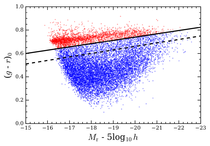
Galaxies in eagle show similar colour bi-modality as those in gama (Trayford et al., 2015, and Trayford in prep.): a blue cloud of star forming galaxies and a red sequence of mostly passive galaxies. In the simulation, the appearance of passive red galaxies is due to the suppression of star formation in satellites and by feedback from supermassive black hole, as demonstrated by Trayford et al. (2016). The colour cut used by Farrow et al. (2015) to separate red from blue galaxies in gama is (their Eq. 4)

$$(g-r)_{0}=0.618-0.03\,(M_{r,h}+18.6)\,,\,\,\,\,\hbox{({\sc gama}\ red-blue cut)}\,,$$ (1)

shown as a dashed black line on the rest-frame colour-magnitude plot of Fig. 1. Here we separate eagle galaxies in a red and blue population using

$$(g-r)_{0}=0.7-0.028\,(M_{r,h}+18.6)\,\,\,\,\hbox{({\sc eagle}\ red-blue cut)}\,,$$ (2)

shown as the black line in Fig. 1. Therefore, the aim of the colour cut is to separate the passive from the active population of galaxies. It is essential to ensure that comparable cuts are made in the different data sets. The slope of observed and simulated colour cuts are virtually identical, and they are offset in colour by less than 0.1 magnitude at $M_{\rm r,h}=-18.6$. This offset is comparable to the offset of $\sim 0.15$ (but in the opposite direction to the eagle offset) for the semi-analytical model considered by Farrow et al. (2015) (see their Fig. 2).

2.2 Dark Matter only simulations

We use two dark matter only simulations to study the impact of the limited simulation volume of the eagle simulation on clustering, one with the same volume and initial conditions as eagle (referred to as eagle-dmo below, this is the simulation L00100N1504-DMO described by Schaye et al., 2015) and one with a much larger simulation volume (referred to as p-millennium below). Combined they allow us to asses to what extent missing large-scale power and sample variance affect inferences on clustering from the relatively small eagle volume.

Simulation eagle-dmo has the same volume, gravitational softening, cosmology and initial conditions as eagle. The masses of the dark matter particles are increased by a factor of $(\Omega_{\rm b}+\Omega_{\rm dark})/\Omega_{\rm dark}$ compared to eagle, to account for not including the baryonic mass. We use this simulation to study clustering of haloes compared to other models - without results being affected by galaxy formation. The impact of baryonic effects on the density profiles of haloes in eagle was investigated by Schaller et al. (2015).

The p-millennium simulation (see Table 1; Baugh et al. in prep. and McCullagh et al. in prep. ) uses identical cosmological parameters as eagle but has a much larger volume (800³Mpc³ compared to the 100³Mpc³ for the eagle simulation used here). With p-millennium we can quantify the effects of missing large-scale power and poor sampling of long wavelengths on clustering statistics by comparing the dark matter halo clustering in eagle-dmo with p-millennium. For details about p-millennium see Baugh et al. in prep and McCullagh et al. in prep.

In both eagle-dmo and p-millennium, dark matter haloes were identified using the friends-of-friends (FoF) algorithm with the standard value of $b=0.2$ for the linking length in units of the mean particle separation. The mass of the halo is represented by $M_{200,c}$, the mass enclosed within a sphere with a density 200 times the critical density.

2.3 The gama survey

To put the eagle simulation results into context, we will compare them primarily to results from the gama survey data, and in particular to clustering measurements made by Farrow et al. (2015). The Galaxy And Mass Assembly (gama) survey (Driver et al., 2011; Liske et al., 2015) is a spectroscopic and multi-wavelength survey of galaxies carried out on the Anglo-Australian telescope. In this work, we make use of the main r-band limited data from the gama equatorial regions ($\sim$180 sq.deg.), which consists of a highly complete ($>98$ per cent) spectroscopic catalogue of galaxies selected from the SDSS DR7 (Abazajian et al., 2009) to $r_{\rm petro}<19.8$. Further details of the gama survey input catalogue, tiling algorithm, redshifting and survey progress are described by Baldry et al. (2010), Robotham et al. (2010), Baldry et al. (2014) and Liske et al. (2015), respectively.

For the clustering comparisons presented in § 4, we are primarily interested in the following gama galaxy properties: r-band absolute magnitude, stellar mass and rest-frame $(g-r)_{0}$ colour. We describe in turn how each of those properties have been estimated in the clustering measurements of Farrow et al. (2015).

• r-band absolute magnitude ($M_{r,h}$): we apply evolution corrections and k-corrections to $z_{\rm ref}=0$ Petrosian r-band absolute magnitudes, where $M_{r,h}\equiv M_{r}-5\,log_{10}(h)$. For further details, see § 2.1.4 of Farrow et al. (2015).

• $(g-r)_{0}$ colour: the rest-frame colours are derived from SDSS model magnitudes, with colour and redshift dependent k-corrections as per Loveday et al. (2012) and McNaught-Roberts et al. (2014). For further details, see § 2.1.4 of Farrow et al. (2015).

• stellar mass ($M_{\star}$ in units of $h^{-2}$M_⊙): the clustering measurements in Farrow et al. (2015) use the relation between rest-frame $(g-i)_{0}$ colour and stellar mass as derived by Taylor et al. (2011), using the Bruzual & Charlot (2003) synthetic stellar population models with a Calzetti et al. (2000) dust attenuation law to correct for dust in the Milky Way. For further details, see § 2.1.5 of Farrow et al. (2015) and Taylor et al. (2011).

For completeness, we refer the reader to § 3 of Farrow et al. (2015) for the modelling of the gama selection function. Accurate modelling of the selection function of a redshift survey is key for precise clustering measurements. The modelling approach described in Farrow et al. (2015), which is based on the method of Cole (2011), enables a uniform modelling for all galaxy samples split by stellar mass, luminosity and colour.

3 Galaxy clustering

In this section we present the analysis methods used, starting with the estimators we use for calculating the two-point correlation function and its associate errors. We then briefly discuss how we compute the effective bias.

3.1 The two-point correlation function

The spherically averaged two-point correlation function, $\xi(r)$, defined as (e.g. Peebles, 1980)

$$\xi(r)={1\over\langle n\rangle}\,{{\rm d}P\over{\rm d}V}-1\,,$$ (3)

provides a statistical description of a sample’s spatial distribution. Here, ${\rm d}P/{\rm d}V$ is the probability of finding a galaxy in the volume ${\rm d}V$ at a given (co-moving) distance $r$ from another galaxy, and $\langle n\rangle$ is the mean (co-moving) number density of galaxies. In practice for a volume with periodic boundary conditions, the correlation function can be estimated by counting the number of pairs of galaxies, $N_{s}(r)$, in a shell of volume $V_{s}(r)$ at distance $r$ from each other using (e.g. Rivolo, 1986)

$$\xi(r)=\frac{1}{\langle n\rangle^{2}V}\frac{N_{s}(r)}{V_{s}(r)}-1\,,$$ (4)

where $V$ is the total volume of the periodic simulation.

However, when the volume has boundaries (as is the case for any observed survey, or when we want to restrict the analysis to a small region within a larger periodic simulation volume), these equations cannot be used. In such cases, $\xi$ can be computed by comparing the distribution of galaxy pairs to the clustering of a set of points uniformly distributed within the survey volume, using e.g. the Landy & Szalay (1993) estimator:

$$\xi(r)=\frac{DD-2DR+RR}{RR}\,,$$ (5)

where $DD$ is the suitably normalised number of galaxy pairs at a distance $r$ from each other, $RR$ the corresponding normalised number of pairs from the random distribution, and $DR$ the suitably normalised numbers of galaxies and random pairs separated by distance $r$.

The co-moving distance between galaxies cannot be measured directly from a redshift survey due to galaxy peculiar velocities and large-scale redshift space distortions. However, by splitting the information into projected separation, $r_{p}$, and distance parallel to the line of sight, $\pi$, one can estimate the 2D correlation function, $\xi(r_{\rm p},\pi)$, which in turn is used to estimate the projected correlation function,

$$w_{p}(r_{\rm p})=2\int_{0}^{\pi_{\rm max}}\xi(r_{\rm p},\pi)d\pi\,,$$ (6)

with $\pi_{\rm max}$ set to a value adequate for the sample considered (here $\pi_{\rm max}$ is fixed to $\sim 34$ Mpc/$h$, which represents $\sim L/2$ of eagle simulation. See Table 1). We select $\pi_{\rm max}$ to be sufficiently large to account for most redshift space distortions. In addition the $\pi_{max}$ value chosen is in line with what is commonly used in observational clustering measurements. To a very good approximation, $w_{p}(r_{\rm p})$ is independent of redshift space effects, making this statistic ideal for model comparisons. Furthermore, we tested the systematic differences between $\xi(r)$ and $w_{p}(r_{\rm p})$ and their dependence on $\pi_{max}$, finding that the systematic difference is significantly smaller than the statistical errors. We compute $w_{p}(r_{\rm p})$ along three orthogonal directions in the simulations, to improve the signal-to-noise of the clustering measurements.

To reduce the dynamical range when plotting $w_{p}$, we will often divide by the projected correlation function of the reference power law, $\xi(r)=(r_{0}/r)^{\gamma}$ with $r_{0}=5.33h^{-1}{\rm Mpc}$ and $\gamma=1.8$, from Zehavi et al. (2011) for the galaxy sample with $-21.0<M_{r,h}<-20.0$, and where the constants are from the fit function that corresponds to this power-law is

$$w_{p}^{\rm ref}(r_{\rm p}) = r_{\rm p}\big{(}\frac{r_{\rm 0}}{r_{p}}\big{)}^{\gamma}\frac{\Gamma(1/2)\Gamma((\gamma-1)/2)}{\Gamma(\gamma/2)}\,,$$ (7)

where $\Gamma$ denotes the Gamma function.

3.2 Error estimates on clustering statistics

We compute and quote jackknife errors on the simulated two-point correlation function in eagle to mimic observational errors. However, sample variance is likely to dominate the error budget. We estimate sample variance by sub-sampling eagle sized-volumes in the p-millennium simulation, which also allows us to examine any effects due to missing large-scale power. Unfortunately we can only estimate these errors for the clustering of haloes - not galaxies - since the p-millennium simulation is dark matter only.

We apply the jackknife technique by partitioning the eagle (or eagle-dmo) simulation volume in $N_{\rm sub}$ tiles of equal volume, with $N_{sub}=8$. We then compute the two-point correlation function $\xi^{JK}_{k}$ by omitting the $k$-th tile, and compute the variance

$$\sigma^{2}(r)=\frac{(N_{\rm sub}-1)}{N_{\rm sub}}\sum_{k=1}^{N_{\rm sub}}(\xi^{JK}_{k}(r)-\xi^{\rm tot}(r))^{2}\,,$$ (8)

where $\xi^{\rm tot}(r)$ is the correlation function of the total volume. Such jackknife error estimates have been used extensively to estimate errors in galaxy clustering (e.g., Zehavi et al., 2002, 2011; Favole et al., 2016), and Zehavi et al. (2002) shows that such errors accurately reflect uncertainties in the clustering on the scales investigated here. However, it has of course its limitations, as pointed out by e.g. Norberg et al. (2009). For example the technique may underestimate errors when a few systems dominate the signal. We will see below this is in fact the case in eagle, where the clustering of low-mass red galaxies on small scales is dominated by satellites in a few massive clusters, as we illustrate in Fig. 7 below.

We estimate errors on the clustering of haloes due to sample variance and missing large-scale power on eagle volumes using the p-millennium simulation as follows. We partition the p-millennium simulation in $N_{\rm sub}=512$ tiles of volume equal to that of eagle. We then calculate the correlation function of haloes in the $i$-th tile, $\xi_{i}(r)$, using Eq. (5), as well as the correlation function of the total volume, $\overline{\xi}(r)$. The variance is then calculated as

$$\sigma^{2}(r)=\frac{1}{{N_{\rm sub}-1}}\sum_{i=0}^{N_{\rm sub}}(\xi_{i}(r)-\overline{\xi(r)})^{2}\,.$$ (9)

We use the number density of haloes of each non-overlapping tile to compute $\xi_{i}(r)$.

3.3 Effective bias

The bias, $b$, of a tracer population is the ratio of the correlation function of that tracer over that of the mass (e.g. Davis et al., 1985), with the effective bias, $b_{\rm eff}(X)$, given by (e.g. Porciani et al., 2004)

$$b_{\rm eff}(X)=\frac{\int b(M_{h})\,N_{gal}(M_{h},X)\,n(M_{h})\,dM_{h}}{\int N_{gal}(M_{h},X)\,n(M_{h})\,dM_{h}},$$ (10)

where $n(M_{h})$ is the halo mass function (the number density of haloes of mass $M_{h}$), $b(M_{h})$ the linear bias factor of haloes of mass $M_{h}$, and $N_{\rm gal}(M_{h},X)$ the mean number of galaxies of property X in haloes of mass $M_{h}$ (the mean halo occupation). The property $X$ could select galaxies in a given stellar mass, colour or luminosity range, for example. We approximate the integral as a sum over all haloes in the simulation, obtaining

$$b_{\rm eff}(X)=\frac{\sum_{i=0}^{N_{\rm haloes}}b(M_{h}^{i})N_{\rm gal}(M_{h}^{i},X)}{\sum_{i=0}^{N_{\rm haloes}}N_{\rm gal}(M_{h}^{i},X)}\,,$$ (11)

where $N_{\rm gal}(M_{h}^{i},X)$ is the number of galaxies with property X in a halo of mass $M_{h}^{i}$. In practice we estimate the effective bias of samples split by stellar mass and hence evaluate this sum for all galaxies in narrow stellar mass bins.

To estimate the linear halo bias $b(M_{h})$, we follow Mo & White (1996),

$$b(M_{h})=1+(\nu(M_{h})^{2}-1)/\delta_{c}\,,$$ (12)

where $\delta_{c}=1.686$ is the spherical collapse density threshold, and $\nu(M_{h})={\delta_{c}}/{\sigma(M_{h})}$ the dimensionless amplitude of fluctuations that produce haloes of mass $M_{h}$ (at a given redshift $z$). The (linear) matter variance, $\sigma(M_{h})$ at a given $z$, can be computed numerically for a given linear power spectrum (see Eq. (9) in Murray et al., 2013) using the web-portal HMFcalc (and adopting the spectral index $n_{s}=0.9611$ used in eagle). Finally, we adopt the fit provided by Jenkins et al. (2001) for the halo mass function, $n(M_{h})$, which provides a good description of the halo mass function of all simulations used here.

4 Results

We begin by considering the clustering of dark matter haloes in eagle, followed by a quick look at the real and redshift space clustering of eagle galaxies with well resolved stellar mass. In §4.3 we present the main results of this study, namely the clustering of galaxies in eagle compared to that of gama, when split by stellar mass, luminosity, colour or star-formation rate.

Figure 2: The $z=0$ real space two-point correlation function of haloes with mass $M_{h}>10^{12}{\rm M}_{\odot}h^{-1}$ from p-millennium (black dashed line), the mean correlation function, $\overline{\xi}(r)$, of the 512 non-overlapping tiles of that simulation (grey line), and the 1$\sigma$ scatter around this mean (computed with Eq. 9, grey error bars). The green curve is the correlation function for simulation eagle-dmo with jackknife error bars. Finite-volume effects cause the green curve to fall increasingly below the grey line, with jackknife errors yielding nevertheless a realistic error estimate.

4.1 Halo clustering in EAGLE

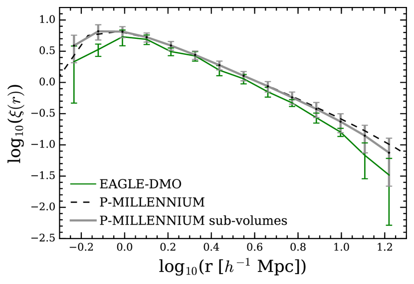
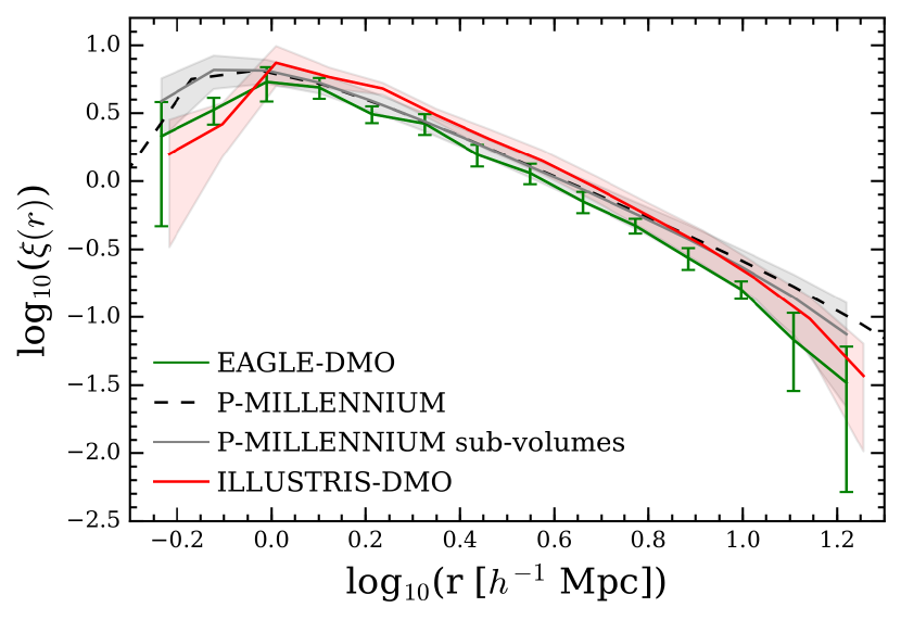
The real-space clustering of haloes with $M_{h}>10^{12}\,h^{-1}{\rm M}_{\odot}$ in the p-millennium dark matter simulation is plotted in Fig. 2. We sub-divide the volume of this simulation into 512 non-overlapping tiles, each with the same volume as eagle-dmo, and compute the correlation function $\xi_{i}(r)$ for each of the tiles, using the mean number density of haloes in each tile in Eq.(5). We plot the mean correlation function averaged over all tiles, $\overline{\xi}(r)$, as the grey line, with the scatter around the mean shown as $1\sigma$ error bars. The mean correlation function $\overline{\xi}(r)$ follows the correlation function of the full volume (black dashed line) very closely, falling well within the scatter between volumes, as expected.

The correlation function of eagle-dmo (green line) falls below $\overline{\xi}(r)$ on scales smaller than $1~{}h^{-1}$ Mpc, remains well within sample variance up to scales $5-6~{}h^{-1}$ Mpc ($\log r/(h^{-1}{\rm Mpc})=0.7-0.78$), then falls increasingly below $\overline{\xi}(r)$ above this scale. As both simulations have identical power-spectra and cosmological parameters, the deviations are due to sample variance and to the integral constraint on $\xi$. We note that numerical resolution is not likely to play a role in the apparent differences in clustering, as these haloes are resolved by $\approx 10^{4}$ particles or more.

We compute jackknife errors for eagle-dmo, as described above, and plot them in green. Of course these do not quantify finite-volume effects nor sample variance, but nevertheless the green and black curves are within the eagle-dmo jackknife errors. This motivates us to use such errors when calculating errors on the correlation function of galaxies, rather than haloes, below, since we do not have access to larger hydrodynamical simulations to estimate finite-volume effects. Given the level of convergence between eagle-dmo and p-millennium, we will plot correlation functions up to scales of 10$~{}h^{-1}$ Mpc (14 per cent of the full extent), with Fig. 2 quantifying the limitations on halo clustering.

4.2 Galaxy clustering in eagle

Figure 3: Top panel: the $z=0.1$ two-point correlation function for eagle galaxies with $M_{\star}>10^{8.66}h^{-2}{\rm M}_{\odot}$ (green curve with jackknife errors bars), decomposed in the one- and two-halo terms (dashed and dotted grey lines, respectively). The red line is the reference power law model for galaxies with $-21.0<M_{r,h}<-20.0$ from the fit by Zehavi et al. 2011. Bottom panel: corresponding projected correlation function, $w_{p}(r_{p})$ from Eq. (6). The red line is the projected correlation function from the fit by Zehavi et al. 2011, $w_{p}^{\rm ref}$ from Eq. (7). The galaxy selection is different in detail for eagle and the observations: the red lines are shown to guide the eye.

Figure 4: The $z=0.1$ two-dimensional redshift space correlation function $\xi(r_{\rm p},\pi)$, as function of projected separation $r_{\rm p}$ and line-of-sight separation $\pi$, for eagle galaxies with stellar masses greater than $10^{8.66}h^{-2}{\rm M}_{\odot}$. Contours levels correspond to $\xi(r_{p},\pi)=5,2,1,0.5,0.2,0.1,0.01$. The vertical dashed line corresponds to projected separations of $r_{p}=10h^{-1}{\rm Mpc}$ beyond which the clustering of haloes is increasingly suppressed due the limited extent of the eagle simulation (see Fig. 2).

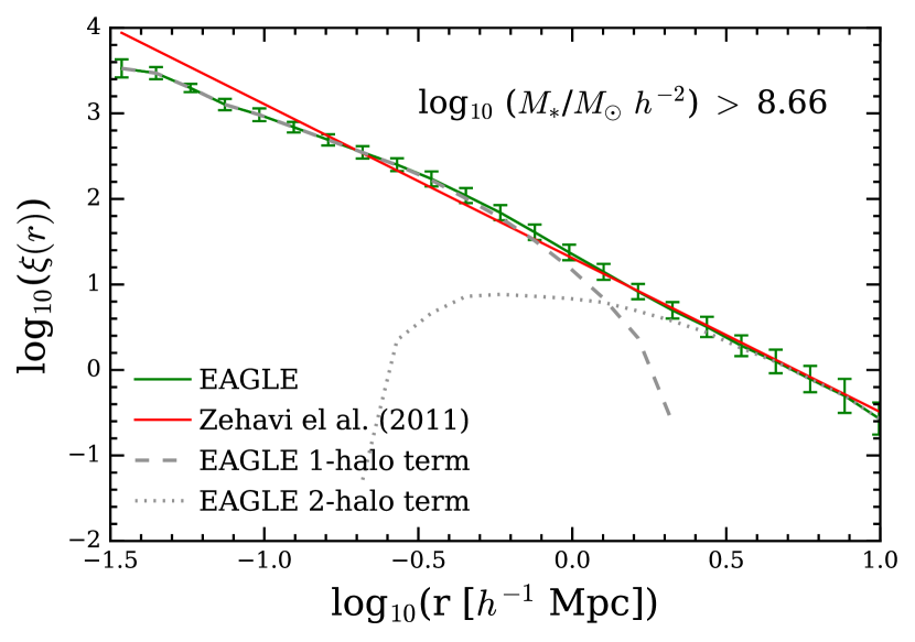
The real-space correlation function, $\xi(r)$, of galaxies with stellar mass $M_{\star}>10^{8.83}h^{-2}{\rm M}_{\odot}$ from eagle is plotted in Fig. 3 (top panel). Distinguishing between central galaxies (typically but not necessarily the most massive galaxy in a given halo) and satellites galaxies, we compute the one- and two-halo contributions separately (grey dashed and grey dotted lines, respectively). The contribution to $\xi$ from these is equal at a separation of approximately $r=1.3~{}h^{-1}$ Mpc. It is important to note that, while the two-point correlation function from the dark matter haloes of eagle-dmo is underestimated at distances below $r\sim 1\,h^{-1}{\rm Mpc}$, this does not imply that the same is true for the galaxy correlation function, since there are of course generally many galaxies per halo.

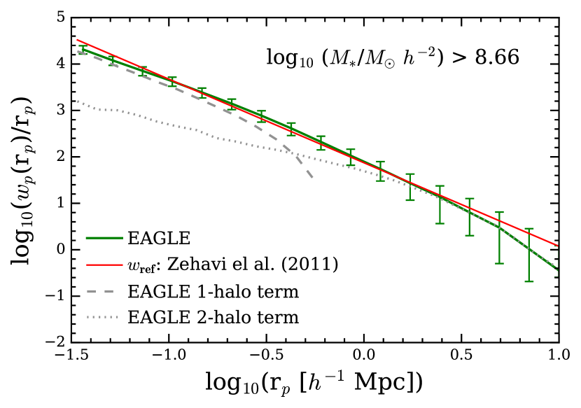
The real-space correlation function quantifies the physical clustering of galaxies, independently of any peculiar velocities. However, observations can only measure clustering in redshift space, and peculiar velocities then distort the signal. To ameliorate the effects of such redshift space distortion, it is convenient to integrate $\xi(r_{p},\pi)$ over a narrow range in $\pi$, and compute the projected correlation function $w_{\rm p}(r_{\rm p})$, see Eq.(6). This is plotted for the same eagle galaxies (those with $M_{\star}>10^{8.83}h^{-2}{\rm M}_{\odot}$) in the bottom panel of Fig. 3, again plotting one- and two-halo terms as well.

The reference model $w_{p}^{\rm ref}(r_{\rm p})$ of Eq. (7) provides a relatively good fit to eagle’s projected correlation function. We note, however, that the galaxy selections differ between eagle and the sdss galaxies fit by Zehavi et al. (2011) that gives rise to $w_{p}^{\rm ref}$ – the two therefore did not have to agree: we show the comparison to guide the eye, and because we use $w_{p}^{\rm ref}$ as a normalisation below.

The contribution of one- and two-halo terms to $w_{p}$ are equal at a projected separation of $r_{p}\sim 0.4h^{-1}{\rm Mpc}$. Comparing top and bottom panel from Fig. 3, it is clear that the two-halo term contributes more to the the projected correlation function on scales comparable to the virial radius of haloes than it does to the two-point correlation function: at a scale of $\approx 0.1h^{-1}{\rm Mpc}$, the two-halo term contributes nearly 10 per cent to $w_{p}$.

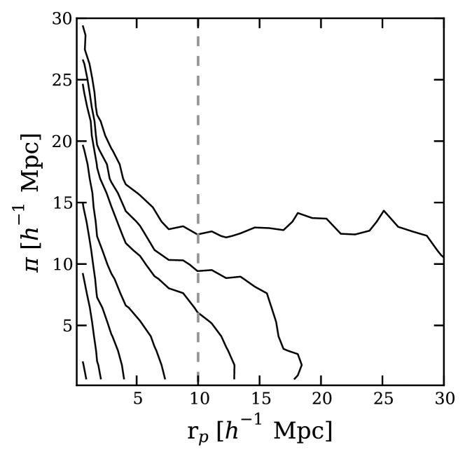
The two-dimensional redshift space correlation function of this stellar mass limited sample of eagle galaxies is plotted in Fig. 4 in terms of the projected separation, $r_{p}$, and line of sight separation, $\pi$. It exhibits the familiar elongation in the $\pi$ direction at small $r_{p}$ resulting from virial motion of galaxies in haloes (the ‘fingers-of-god’ effect), and the flattening in the $\pi$ direction at large $r_{p}$, due to coherent streaming motions of galaxies into haloes and out of voids (the ‘Kaiser’ effect, Kaiser (1987)). We do not compare this correlation function directly to gama, mainly because of the complexity of making sure the selection of galaxies in the $\pi$ direction is the same in simulation and data.

4.3 Galaxy clustering in eagle compared to gama

We use the volume-limited samples of gama galaxies presented by Farrow et al. (2015), which we can split by stellar mass, luminosity or colour. For samples split in bins of stellar mass or luminosity only, we refer the reader to Table 2 of Farrow et al. (2015), while we present in Table 2 the properties of the additional gama samples used in here, for which we have computed clustering statistics following the methods outlined by Farrow et al. (2015).

Throughout this section, eagle galaxies are selected from the $z=0.1$ snapshot (a redshift close to the median redshift of the gama samples). Some statistics of the eagle samples used are provided in Table 3. By construction and as explained in Section 2.1, the galaxy formation model in eagle yields a stellar mass function that is in relatively good agreement with that inferred from gama in the mass range we analyse here. The agreement is not as good as in statistical methods that populate dark matter halos with galaxies, such as sham or hod for example, and which yield the correct number densities by construction. Interestingly however, eagle predicts a scatter in stellar mass at a given halo mass that depends on halo concentration, although the dependence is not strong enough to explain the full variance (Matthee et al., 2017). Such non-linear dependencies are not taken into account in these statistical methods.

Hence, because the mean number density of galaxies in each bin of stellar mass, agree reasonably well between data and simulation, we do not compare clustering at given number density, as commonly done, but directly compare samples selected by stellar mass - or indeed luminosity.

Figure 5: Clustering as a function of stellar mass; the mass bin is indicated in each column. Top panels: Projected correlation function $w_{p}(r_{p})$ from Eq. (6). Green curve is the eagle result at $z=0.1$, with jackknife error bars; $N_{\rm gal}$ is the number of eagle galaxies in each mass bin. Black curve is gama result, with the grey shading including the 1-$\sigma$ error range. Bottom panels: Same as top panels, but the correlation functions are divided by the reference function $w^{\rm ref}_{p}(r_{p})$ from Eq. (7). The dashed line indicates where the ratio is unity.

Figure 6: Same as the bottom panels of Fig. 5, but for clustering as a function of $r$-band luminosity. Ranges of $r$-band absolute magnitudes are shown from faint to bright (top to bottom panels), with the number of eagle galaxies in this luminosity range labelled in each panel. The jackknife error bars for eagle galaxies are included.

Table 2: Statistics of gama galaxy samples (mostly volume limited), that are not already described in Table 2 of Farrow et al. (2015), following a similar table structure. The stellar mass restricted samples are split into red and blue galaxies, presented in turn. Columns from left to right are: stellar mass range, minimum and maximum sample redshift, total number of galaxies, the galaxy number density, median sample redshift, median $r$-band absolute magnitude, median stellar mass, median $(g-r)_{0}$ rest-frame colour, and the fraction of truly volume limited galaxies (see text for further details).

stellar mass range	$z_{\rm min}$	$z_{\rm max}$	Ngals	$\bar{n}$	$z_{\rm med}$	M${}^{\rm med}_{r,h}$	$\log_{10}$ M${}_{*}^{\rm med}$	$(g-r)^{med}_{0}$	$f_{vlim}$
				$({\rm Mpc}/h)^{-3}$			$(h^{-2}\,{\rm M}_{\odot})$
Red
$9.5<\log_{10}{\rm M}_{*}/h^{-2}\,{\rm M}_{\odot}<10.0$	0.02	0.14	5407	4.45 10-3	0.11	-19.16 (0.38)	9.77 (0.14)	0.72 (0.07)	0.96
$10.0<\log_{10}{\rm M}_{*}/h^{-2}\,{\rm M}_{\odot}<10.5$	0.02	0.14	5527	4.55 10-3	0.11	-20.16 (0.40)	10.23 (0.14)	0.75 (0.10)	1.00
$10.5<\log_{10}{\rm M}_{*}/h^{-2}\,{\rm M}_{\odot}<11.0$	0.02	0.14	1945	1.60 10-3	0.12	-21.11 (0.37)	10.65 (0.12)	0.77 (0.09)	1.00
Blue
$9.5<\log_{10}{\rm M}_{*}/h^{-2}\,{\rm M}_{\odot}<10.0$	0.02	0.14	4663	3.84 10-3	0.11	-19.71 (0.39)	9.71 (0.14)	0.54 (0.08)	1.00
$10.0<\log_{10}{\rm M}_{*}/h^{-2}\,{\rm M}_{\odot}<10.5$	0.02	0.14	1870	1.54 10-3	0.12	-20.61 (0.34)	10.18 (0.13)	0.61 (0.06)	1.00
$10.5<\log_{10}{\rm M}_{*}/h^{-2}\,{\rm M}_{\odot}<11.0$	0.02	0.14	248	0.20 10-3	0.12	-21.44 (0.34)	10.61 (0.11)	0.67 (0.06)	1.00

Table 3: Statistics of eagle stellar mass selected samples from the $z=0.1$ snapshot. Columns from left to right are: stellar mass range, number of galaxies, galaxy number density (including JN errors), fraction of satellites, fraction of blue galaxies (following Eq. 2), the SFR limits used to define ‘low’ and ‘high’ SFR galaxy samples respectively, number density of red and blue galaxies, respectively.

Sample	Ngals	$\bar{n}$	$f_{\rm sat}$	$f_{\rm blue}$	SFRlow	SFRhigh	$\bar{n}_{\rm red}$	$\bar{n}_{\rm blue}$
stellar mass range		$({\rm Mpc}/h)^{-3}$			${\rm M_{\odot}\,yr^{-1}}$	${\rm M_{\odot}\,yr^{-1}}$	(Mpc/$h$)-3	(Mpc/$h$)-3
9.5$<\log_{10}{\rm M}_{*}/h^{-2}\,{\rm M}_{\odot}<$10.0	2676	(8.6$\pm$0.9) 10-3	0.43	0.82	$<$0.28	1.02$<$	1.5 10-3	7.1 10-3
10.0$<\log_{10}{\rm M}_{*}/h^{-2}\,{\rm M}_{\odot}<$10.5	1460	(4.7$\pm$0.5) 10-3	0.39	0.77	$<$0.26	1.99$<$	1.2 10-3	3.6 10-3
10.5$<\log_{10}{\rm M}_{*}/h^{-2}\,{\rm M}_{\odot}<$11.0	437	(1.4$\pm$0.1) 10-3	0.22	0.81	$<$0.65	3.43$<$	2.7 10-4	1.1 10-3

4.3.1 Stellar mass dependent clustering

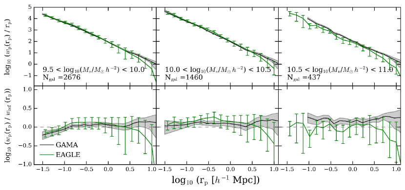
A comparison of the clustering of eagle galaxies to that in gama as a function of stellar mass is shown in Fig. 5, using the same mass as used by Farrow et al. (2015). The bottom panels of Fig. 5 highlight the differences between the two measurements, by presenting the ratio of the projected correlation functions with respect to the reference power law model adopted (following Farrow et al., 2015). The projected correlation function of eagle galaxies (green lines with jackknife errors) is in remarkably good agreement with the gama data (solid black lines, with 1-$\sigma$ uncertainty range shown as a grey shaded area): the deviations are typically within the measured uncertainty range.

It is well known (and clear from the figure) that the clustering strength of galaxies increases with stellar mass. There is little or no evidence for such a trend in the simulation, however the errors are relatively large and the simulation is not inconsistent with such a trend either. Furthermore, the size of the simulation prevents us to test the stellar mass dependent clustering, due to observed trends are only visible when having a large dynamic range of stellar masses. Therefore, a larger volume would be needed to confirm such trend. The good agreement in shape of the correlation functions of gama and eagle is encouraging.

The calibration of sub-grid parameters in eagle was based on one-point statistics, as described in Section 2. The clustering of galaxies is therefore a genuine model prediction. The good agreement then implies that eagle galaxies tend to inhabit haloes in a way that mimics accurately the way gama galaxies do. Finally we note that the decrease of the clustering signal on scales greater than 5 $h^{-1}{\rm Mpc}$ scales in eagle is related to the limited simulation box size - and mimics the corresponding fall in clustering of eagle haloes.

4.3.2 Luminosity dependent clustering

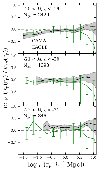
A comparison of the clustering of eagle galaxies to that in gama as a function of $r$-band luminosity, is shown in Fig. 6. The agreement is very good, and well within the relatively large jackknife error estimates. Similar to the case of clustering as function of mass, the amplitude of observed clustering increases with luminosity (see e.g. Norberg et al., 2001; Zehavi et al., 2005), but again there is little or no evidence for such a trend in eagle. As in the previous section, we suggest this is mostly due to the finite volume of the simulation: more luminous galaxies are biased to more massive haloes, of which there are relatively few in the eagle volume, and their clustering is underestimated because of lack of large-scale power. The reference power law $w_{p}^{\rm ref}$ from Eq. (7), describes the clustering of eagle galaxies in the middle panel of Fig. 6 very well. In this panel, eagle galaxies are selected in the same way, $-21.0<M_{r,h}<-20.0$, as in the sample of Zehavi et al. (2011) to which $w_{p}^{\rm ref}$ was fit, so they can be compared directly. The good agreement in clustering, combined with the fact that eagle also fits the galaxy luminosity function well (Trayford et al., 2015), implies that eagle galaxies form in similar haloes, and have similar stellar populations and star formation histories as those in gama. This encourages us to look in clustering as function of galaxy colour in more detail next.

4.3.3 Colour dependent clustering

Figure 7: Clustering as function of $(g-r)_{0}$ colour for red and blue galaxies (left and right column, respectively), in bins of stellar mass (top to bottom rows). Limits of each mass bin are labelled in each panel. The projected correlation function for eagle galaxies in each mass bin is shown by the red and blue curves for red and blue galaxies, respectively, $N_{\rm gal}$ is the number of eagle galaxies that contributes to the calculation. The corresponding clustering of gama galaxies is shown by the black line with grey shaded region the 1-$\sigma$ error range. The clustering of central and satellite eagle galaxies split by mass but not by colour, is plotted as dotted green and dashed green lines, respectively. In the left column, the orange lines are $w_{p}$ of red eagle galaxies, after excluding the three most massive haloes.

Farrow et al. (2015) present $r$-band magnitude limited samples of gama galaxies split by rest-frame $(g-r)_{0}$ colour and in bins of stellar mass. Galaxies are classified as ‘red’ or ‘blue’ using the $r$-band magnitude colour cut of Eq. (1). We use this data to compute $w_{p}$ for these galaxies using the method described by Farrow et al. (2015). Some statistics of these samples are summarised in Table 2. We note that the lowest mass bin in red galaxies, $9.5<\log_{10}{\rm M}_{*}/h^{-2}\,{\rm M}_{\odot}<10.0$, is only partially volume limited, as $\sim 4$ per cent of the galaxies in that sample are only volume limited over a smaller redshift range than the one nominally considered. Given the small galaxy fraction affected by this, we can consider this sample still to be volume limited when computing clustering statistics. The advantages of keeping the exact same volumes for all stellar mass samples split by colour (hence they all sample the same underlying large scale structure) overcomes this minor subtlety, which is primarily driven by uncertainties in the measured colours and adopted k-corrections for a small subset of galaxies.

We computed colours of eagle galaxies as explained in Section 2.1. The colour-magnitude diagram exhibits a blue cloud of star forming galaxies, well separated from a ‘red sequence’ of passive galaxies, as shown by Trayford et al. (2015) (see also Trayford et. al. 2017, submitted). The colour of eagle’s red sequence is slightly bluer than in gama, which may due to differences in metallicity and/or limitations in the adopted population synthesis models, as discussed by Trayford et al. (2015). When comparing to gama, we want to study whether the clustering of star forming (blue) galaxies differs from that of passive (red) galaxies, at a given mass. We therefore divide eagle galaxies in bins of stellar mass and colour using the same mass bins as used in the analysis of gama, but applying the slightly different colour cut to distinguish red from blue using Eq. (2), as compared to the cut of Eq. (1) applied to gama. Some statistics of the eagle galaxies are summarised in Table 3, including the fraction of eagle galaxies that are satellites.

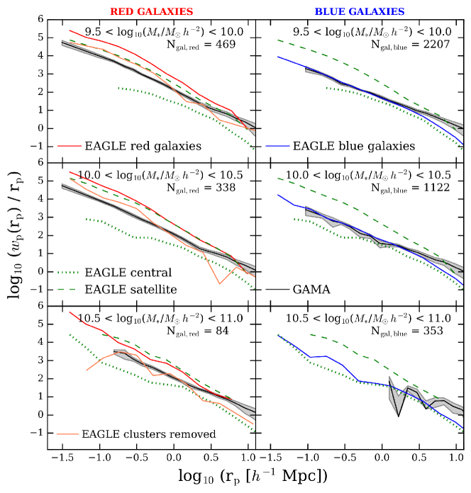
The projected correlation functions for red and blue galaxies, split in bins of stellar mass, is plotted in Fig. 7. To ease the interpretation of the eagle clustering results, we show the correlation function for all central and satellite galaxies (i.e. irrespective of colour) within each stellar mass bin as green dotted and dashed lines respectively. Therefore, the central/satellite clustering results are the same in the left and right panels, but vary with stellar mass (from top to bottom).

In eagle, red galaxies (left column) cluster more strongly than blue galaxies (right panel) of given mass, and similarly satellite galaxies (dashed lines) cluster more strongly than centrals (dotted lines), in all stellar mass ranges studied. It is also apparent that the red population follows closely the clustering of satellites, in particular for galaxies with stellar masses greater than 10${}^{10}h^{-2}{\rm M}_{\odot}$. In contrast, blue galaxies follow more closely the clustering of centrals, again particularly so for the two more massive galaxy stellar bins.

The clustering of blue eagle galaxies tracks that of blue gama galaxies well, in particular on scales up to $r_{p}\sim$4 $h^{-1}$Mpc ($\log_{10}(r_{p})=0.6$). However, red eagle galaxies cluster noticeably more strongly than red gama galaxies. As a consequence, the trend that red galaxies cluster more strongly than blue galaxies of given mass, which is clearly present in gama, is too strong in eagle. Trayford et al. (2015) noticed that red galaxies are overabundant in eagle at low mass, and demonstrated that this is at least partly due to lack of numerical resolution (see the Appendix of Trayford et al., 2015). At higher stellar masses, eagle yields a too large fraction of blue galaxies instead, plausibly a consequence of the dust screen not suppressing blue light from star forming regions sufficiently (Trayford et al. 2017, submitted). We suspect therefore that it is the overly strong suppression of star formation in small galaxies as they become satellites, most likely as a consequence of lack of numerical resolution, that cause eagle to over predict small-scale clustering of red galaxies. Consistent with this interpretation, we find that the strong clustering of red galaxies in eagle is significantly influenced by the presence of a few massive haloes. To demonstrate this, we re-compute $w_{p}$ for red eagle galaxies after excluding all galaxies in the three most massive haloes. We show the result by the orange line in Fig. 7. The overall amplitude of the clustering signal of red galaxies is dramatically reduced. A larger simulation box is likely required to provide detailed insight on the clustering of red massive galaxies.

The colour dependences of the clustering of eagle galaxies of given stellar mass is clearly partly due to the relative fractions of satellite and central galaxies. In Table 3 we show the fraction of satellites and blue galaxies for each stellar mass range. We find that the fraction of satellite galaxies decreases at higher masses, while the fraction of red and blue satellites is not strongly dependent on stellar mass. For example, in the stellar mass range $9.5<\log M_{*}/{\rm M}_{\odot}h^{-2}<10.0$ we find that $\sim 19$% are red and the remaining $\sim 81$% blue, while 43% of the galaxies are satellites. The table also shows that the vast majority of galaxies are blue, but also the most of galaxies of the complete sample in this stellar mass bin are centrals. Furthermore, the good agreement with gama in the clustering of blue galaxies is consistent with the fact that eagle galaxies of given mass cluster similarly to gama galaxies, as shown in Fig. 5. A relatively modest improvement of the numerical resolution of the simulation could be enough to reproduce the clustering of red galaxies equally well (see, Trayford et al., 2015, for further details). However the difference seen could equally be due to the missing large-scale power and the impact the few rare objects have in the 100 Mpc eagle volume.

4.3.4 Star formation rate dependent clustering

Figure 8: Clustering as function of star formation rate. The projected galaxy correlation function of eagle galaxies, divided by the reference power-law of Eq. (7), is plotted for galaxies in bins of stellar mass, as labelled in each panel. In each galaxy stellar mass bin, we show the result for all galaxies (green line), the 30 per cent least star forming galaxies (‘low SFR’, purple), the 30 per cent highest star forming galaxies (‘high SFR’, blue), and the remainder (‘int SFR’, red). Table 3 lists the corresponding cuts in star formation rate.

Figure 9: Halo occupation distribution of eagle galaxies with stellar mass in the range $9.5<\log(M_{*}/{\rm M}_{\odot}h^{-2})<10.0$. The distribution for all galaxies in that stellar mass range is plotted as the black histogram, which is normalised to unit integral. The red and blue histograms show the fraction of those galaxies that are satellites and centrals, respectively. The coloured histograms integrate separately to the fraction of galaxies that are satellite (red) or central (blue) in this range of $M_{\star}$.

Figure 10: As in Fig. 9, but for eagle galaxies split by star formation rate and for a three ranges in stellar mass as indicated in each panel (with increasing stellar mass from top to bottom). The sample cuts are the same as in Fig. 8 (and listed in Table 3).

Figure 11: Effective bias, estimated using Eq. 11, with jackknife errors for eagle galaxies as a function of stellar mass, for three cuts in specific star formation rate, low (purple), intermediate (red) and high (blue). The sample cuts are the same as in Figs. 8 and 10 and are listed in Table 3.

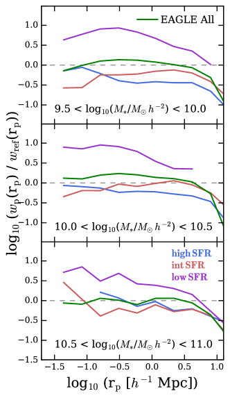
We divide eagle galaxies of a given stellar mass in three bins of star formation rate (SFR), the 30 per cent with the lowest star formation rate (‘low SFR’), the 30 per cent with the highest star formation rate (‘high SFR’), and the remainder (‘int SFR’). Their galaxy clustering is plotted in Fig. 8. The low SFR galaxies are clustered most strongly , which is particularly evident on the smaller scales, and this is the case in all stellar mass bins investigated. The difference in the amplitude of clustering between the high and intermediate SFR galaxies is not very large, with high SFR galaxies generally clustering least. Jackknife errors bars are not plotted to avoid clutter, but should be of order $\pm$0.35 dex (i.e. a factor $\sqrt{3}$ higher than the typical $\pm$0.2 dex errors seen in Fig. 5 below $r_{p}=1h^{-1}$ Mpc). Any difference in clustering between the blue (‘high SFR’) and red (‘int SFR’) curves are therefore not very significant. At the largest scales shown, the amplitude of clustering for all populations becomes similar, with any difference now much smaller than jackknife errors.

We do not compare these clustering measurements to those from gama presented by Gunawardhana et al. (in prep), for the following main reason: the SFR and stellar mass range probed by gama and eagle are in detail poorly matched, in the sense that the limitations in each of the gama and eagle star-forming samples are hard to account for all at the same time. For gama, the SFR is only measurable for galaxies with sufficiently high SFR, resulting in volume limited samples with SFR and stellar mass ranges restricted to SFR $\gtrsim 0.3{\rm M_{\odot}\,yr^{-1}}$ and M${}_{*}\gtrsim 10^{9.5}h^{-2}\,{\rm M}_{\odot}$. (see Gunawardahana et al. (in prep.) for details). Hence for a detailed comparison to take place, it would be necessary to work with samples defined by absolute cuts in SFR. This in turn requires the gama SFR measurements to be directly compatible with those in eagle, as defining samples by SFR ranking is not possible. Although the galaxy number densities of gama and eagle split by stellar mass are in reasonably good agreement, splitting these sub-samples by SFR does not necessarily result in samples with similar number densities, due to differences in the bivariate SFR-M* distribution. In fact we find that the galaxy number densities in eagle are between 60 and 70 per cent larger than in gama for the same stellar mass and SFR range. This implies that a detailed clustering comparison becomes futile: any difference observed in the clustering could be attributed to the differences in the measured number densities of the samples. This is in agreement with the results of Furlong et al. (2015), who pointed out that the specific SFR in EAGLE are typically 0.2 to 0.5 dex lower than observed. A proper understanding of those SFR difference between data and simulations is required before a detailed and informative clustering comparison of SFR selected samples can be made.

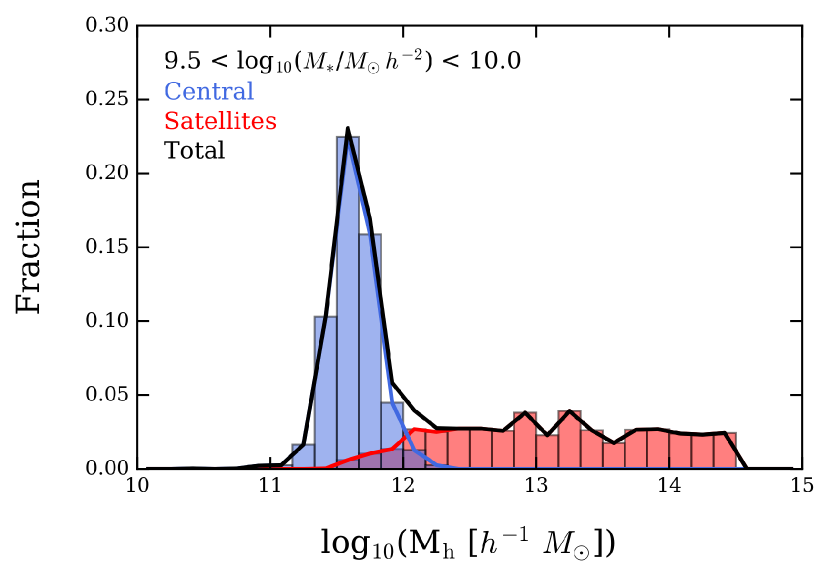
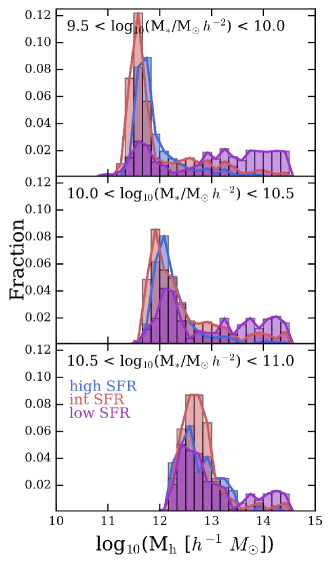
The differences in clustering of galaxies of the same mass that are satellites versus centrals (Fig. 7), or red versus blue galaxies (Fig. 8), should be dependent on the mass of the halo they inhabit, with more strongly clustered galaxies residing in more massive haloes. To verify that this is the case in eagle, we plot the halo occupation distribution - the fraction of galaxies of a given $M_{\star}$ that inhabit haloes of mass $M_{h}$ - for galaxies in the stellar mass range $10^{9.5}<M_{\star}/h^{-2}{\rm M}_{\odot}<10^{10}$ split in centrals and satellites (Fig. 9), or in bins of SFR for three ranges in $M_{\star}$ (Fig. 10).

Central galaxies in the mass range $10^{9.5}<M_{\star}/h^{-2}{\rm M}_{\odot}<10^{10}$, inhabit haloes with a narrow range of masses, from $10^{11.2}h^{-1}{\rm M}_{\odot}$ to $\sim 10^{13}h^{-1}{\rm M}_{\odot}$. In contrast, satellites of the same stellar mass, inhabit haloes with a wide range of masses, from $10^{11}h^{-1}{\rm M}_{\odot}$ to $\sim 10^{14.5}h^{-1}{\rm M}_{\odot}$ (Fig. 9). The (much) stronger clustering of satellites is therefore clearly due to the significant fraction that resides in these much more massive (and hence more clustered) haloes (see e.g., Guo et al., 2014).

At a given stellar mass, eagle galaxies with a higher star formation rate inhabit lower mass haloes than those with a lower value of SFR (at $z=0.1$), as shown in Fig. 10 for three ranges in $M_{\star}$. The figure also demonstrates that the halo occupation is similar for galaxies with a high or intermediate SFR. This explains the results from Fig. 8 that, at given $M_{\star}$, galaxies with a low SFR cluster more strongly than those with higher SFR.

The SFR (and hence also colour) dependence of clustering in eagle is related to the mechanism that causes some galaxies to have a low SFR for their mass: the reduction in SFR once a galaxy becomes a satellite, which is discussed in detail for the eagle simulations by Trayford et al. (2016). The reduction of the SFR of satellites results from two related physical processes that operate in hydrodynamical simulations: ram-pressure stripping, mainly of the outer parts of satellites as shown by Bahé & McCarthy (2015) using the gimic simulations (Crain et al., 2009), and the strong suppression - by many orders of magnitude - of the accretion rate of gas onto satellites shown by Van de Voort et al. (in prep.) in eagle. The much reduced gas fraction of such satellites then also implies that their interstellar medium rapidly increases in metallicity (Bahé et al., in prep.) - a testable prediction of the scenario.

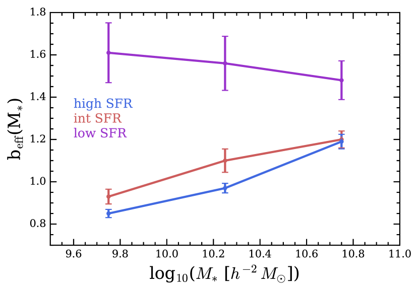
Another way to demonstrate the bias of quenched galaxies to inhabit more massive haloes is shown in Fig. 11, which plots the effective bias of galaxies as function of stellar mass, split by SFR. The effective bias of the low SFR population is nearly independent of $M_{\star}$, and considerably higher than that of the intermediate or high SFR population. For the active galaxies with intermediate or high SFR, the bias increases with stellar mass - simply reflecting that for those galaxies SFR increases with $M_{\star}$, which in turn increases with halo mass.

5 Comparison with other models

Figure 12: Correlation function of $z=0$ of dark matter haloes with mass $M_{h}>10^{12}h^{-1}{\rm M}_{\odot}$ in real space (top panel), and their corresponding projected correlation function divided by a reference power law (bottom panel). Simulations shown are eagle-dmo (green line with jackknife error bars), illustris dark matter only (red line with jackknife errors represented by red shaded area), and p-millennium with line styles as in Fig. 2.

Figure 13: Halo occupation distribution of galaxies at $z=0.1$ in four different stellar mass bins, as indicated in each panel, comparing eagle (green) and illustris (red). With the exception of the lowest stellar mass bin, galaxies of a given mass tend to reside in lower mass haloes in illustris compared to eagle.

Figure 14: Comparison of galaxy clustering between different models and gama, as a function of stellar mass ($M_{\star}$ increases from top to bottom). Different panels show the projected correlation function, $w_{p}(r_{p})$, divided by the reference fit of Eq. (7). The models shown are eagle (green curve with jackknife errors) illustris (red curve - jackknife errors are not shown but are similar to those of eagle), GP14 (dark blue curve) and L14 (cyan curve). The observed correlation function from gama is shown in black with grey shading encompassing jackknife errors. The latter three sets of results are from Farrow et al. (2015). Models GP14 and L14 and gama curves are taken from Farrow et al. 2015

In this section we compare the eagle clustering results to two sets of models: i) two incarnations of the galform semi-analytical model, namely the version of Gonzalez-Perez et al. (2014) (hereafter GP14), and an early version of Lacey et al. (2016) (hereafter L14), both of which were used in the gama clustering study of Farrow et al. (2015); ii) the illustris hydrodynamical simulation described by Vogelsberger et al. (2014).

The galform model assumes that galaxies form in dark matter haloes, and it uses analytical prescriptions to describe galaxy formation processes. These phenomenological prescriptions have free parameters controlling different physical processes necessary for the model to be realistic and which are tuned to fit a set of observational constraints at low redshift. GP14 & L14 use halo merger trees from the millennium-MR7 simulation (Guo et al., 2013), which uses cosmological parameters set by wmap7 (Komatsu et al., 2011). The Gonzalez-Perez et al. (2014) model has the same physical prescriptions as the Lagos et al. (2012) model, but set in a different cosmology to that used by Lagos et al. (2012), resulting in the need to retune the free parameters as described by Gonzalez-Perez et al. (2014). The main differences between GP14 and L14 are: i) the assumed stellar initial mass function, with GP14 using a Kennicutt (1983) IMF, while L14 switches from this IMF to a top-heavy IMF in star bursting galaxies (see Lacey et al., 2016, for further details); ii) the treatment of merging satellite galaxies, with GP14 using the Chandrasekhar dynamical friction timescale in an isothermal sphere as given in Lacey & Cole (1993), while L14 uses the Jiang et al. (2008) and Jiang et al. (2014) formula for the time-scale, which is empirically calibrated on N-body simulations to account for the tidal stripping of the accreting haloes; iii) the assumed stellar population synthesis (SPS) model, with GP14 using an updated version of the Bruzual & Charlot (1993) SPS model, while L14 adopts the Maraston (2005) SPS model. Both GP14 and L14 were tuned to reproduced the b_J-band and K-band luminosity functions of Norberg et al. (2002b) and Cole et al. (2001), respectively. As gama is r-band selected and as Farrow et al. (2015) analysis covered a larger redshift range not probed by those galaxy luminosity functions used to calibrated the GP14 and the L14 galform models, Farrow et al. (2015) adjusted the gama galform lightcone mocks constructed following Merson et al. (2013) to closely reproduce the gama r-band selection function (which in turn is well described by the gama r-band luminosity functions of Loveday et al. (2012, 2015). We note that the L14 model used here and by Farrow et al. (2015) has marginally different parameters from the model discussed by Lacey et al. (2016); we have not investigated whether this impacts any of the results presented below.

The illustris simulation suite was performed with the arepo moving-mesh code of Springel (2010). The simulation volume, $(75h^{-1}{\rm Mpc})^{3}$, is comparable to that of eagle; sub-grid modules for star formation and feedback are as described by Vogelsberger et al. (2014) and the assumed cosmological parameters are close to those of Planck Collaboration et al. (2014) assumed in eagle. Properties of illustris galaxies were released by the collaboration through a database with content described by Nelson et al. (2015). The simulation reproduces several observed properties of galaxies such as for example the colours of satellites (Sales et al., 2015) and the distribution of galaxy morphologies (Snyder et al., 2015). However, the galaxy stellar mass function simulation has an excess of galaxies at both high ($M_{\star}\geqslant 10^{11.5}{\rm M}_{\odot}$) and low ($M_{\star}\leqslant 10^{10}{\rm M}_{\odot}$) stellar masses at redshift $z\leqslant 1$, see Vogelsberger et al. (2014). Here we use the ‘Illustris-1’ run (hereafter illustris) and extract galaxy properties directly from the the illustris database.

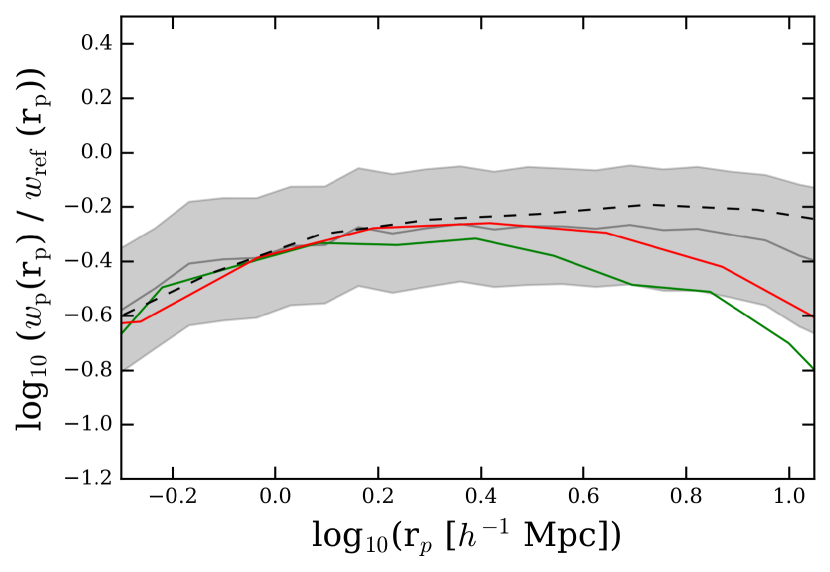
The illustris simulation suite also includes dark matter-only runs. This enables us to compare the clustering of haloes between eagle-dmo and the dark matter-only illustris (Fig. 12). The correlation function of illustris haloes is higher than that of eagle-dmo, both in real and redshift space (except for the smallest scales plotted), with the difference consistent with sample variance as judged from the scatter obtained from eagle like simulation sub-volumes extracted from the significantly larger p-millennium. As discussed before, lack of large-scale power in the smaller boxes and the absence of integral constraint corrections on the clustering estimate cause the correlation functions to drop below that of p-millennium on larger scales.

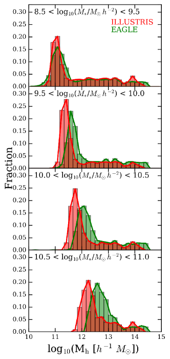
Given that the eagle and illustris dark matter halo functions are very similar, whereas their galaxy stellar mass function are not (see Fig. 5 of Schaye et al., 2015), we expect some differences between the simulations in how galaxies populate the underlying dark matter haloes. This is indeed born-out by Fig. 13: illustris galaxies of given stellar mass prefer lower mass haloes, by about 0.2 dex.

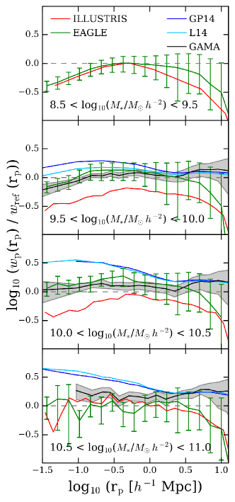
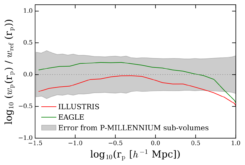
In Figure 14 we compare the two-point correlation function, $w_{p}$, from eagle galaxies with the results from illustris, the GP14 and L14 galform models, and the gama survey, in four stellar mass bins. We divided $w_{p}$ by the reference model $w_{p}^{\rm ref}$ of Eq. (7) to decrease the dynamic range in the plot. The shape of the correlation functions of eagle and illustris are very similar (we do not plot jackknife errors on the illustris curves to avoid clutter, but they are nearly identical to those of eagle), but with illustris offset to smaller values except for the lowest bin in stellar mass (the top panel). The poor sampling of large-scale modes in both hydrodynamical simulations, combined with the integral constraint, may lead to an net offset of $w_{p}$ - as we demonstrated explicitly in Fig. 2 for the dark matter haloes. The level of the offset is consistent with sample variance - as shown by the comparing to the p-millennium results. However, somewhat surprisingly, whereas haloes in illustris are more strongly clustered than those in eagle (red line above green line in Fig. 12), illustris galaxies are less strongly clustered than those in eagle at given $M_{\star}$ (Fig. 14). This is related to the differences in stellar mass function: the galaxy number density is higher in illustris compared to eagle, therefore illustris galaxies of given $M_{\star}$ inhabit haloes of lower mass (Fig.13) which are less clustered. This effect is relatively small, however, and we conclude that the clustering is consistent in both models given the relatively large jackknife errors.

Figure 15: Clustering of the most massive galaxies corresponding to a mean number density of $n_{\rm gal}\sim 1.4910^{-2}h^{3}{\rm Mpc}^{-3}$ at $z=0.1$. The projected correlation function $w_{p}$ is divided by the reference model $w_{p}^{\rm ref}$ of Eq. (7). The eagle and illustris simulations are plotted in green and red, respectively. Sample variance in the clustering of dark matter haloes, mass ranked and selected to have the same mean number density, estimated using from sub-sampling the p-millennium volume, are shown by the grey shaded area (computed with Eq. 9, and including the effective bias of the sample).

We can partially compensate for differences in the stellar mass function of eagle and illustris by comparing galaxy clustering at a given number density, rather than stellar mass. To do so, we select all eagle galaxies with $M_{\star}>10^{9.5}~{}h^{-2}~{}{\rm M}_{\sun}$, yielding a galaxy number density of $n_{\rm gal}\simeq 1.49\times 10^{-2}h^{3}{\rm Mpc}^{-3}$ and then find the corresponding stellar mass range of $M_{\star}>10^{9.73}~{}h^{-2}~{}{\rm M}_{\sun}$ in illustris above which the number density is equal to $n_{\rm gal}$. The clustering of these two samples is compared in Figure 15, with illustris in red and eagle in green, with sample variance in the clustering of dark matter haloes with the same number density estimated by sub-sampling p-millennium volumes in grey. Selected in this way, the clustering in eagle is higher than in illustris, but the differences are consistent with sample variance.

We now turn to the semi-analytical models plotted in Fig. 14. The galform model shown are the average of 26 gama light cone mocks as described in Farrow et al. (2015). Like in that paper, we assume that the errors on those model clustering results are negligible compared to the errors measured on the gama sample. See Farrow et al. (2015) for a quantitative description of how adequate the GP14 and L14 galform models are in describing the observed gama clustering. The correlation functions of GP14 and L14 are very similar, except in the second panel from the top where the GP14 model is above that of L14 on scales below $r_{p}\sim 1h^{-1}$ Mpc. Both models show stronger clustering than observed below $r_{p}\sim 1h^{-1}$ Mpc. As discussed by Farrow et al. (2015), the high values of $w_{p}$ in the galform models are caused by an excess of satellites galaxies and/or their radial distribution in clusters. The satellite merging scheme is the principal mechanism which impacts directly on the number of satellites within haloes. The two versions of galform we use, include the default scheme in which satellite galaxies merge onto the central galaxy after an analytically determined dynamical friction merger time-scale. Campbell et al. (2015) compared the standard galform scheme with a different one (Simha & Cole, 2016), in which the merger time-scale make use of the information from dark matter subhalo of each satellite galaxy. They find that the new scheme reduces the amplitude at small scales and show good agreement with observational results. McCullagh et al. (prep) and Gonzalez-Perez et al. (2017) show that implementing the Simha & Cole (2016) merger scheme within the GP14 model and applying it to the p-millennium simulation results in clustering measurements that are in significantly better agreement with the observed ones on small scales. More detailed studies of the galform clustering predictions on small scales are needed to address the known limitations of samples split by colour (see e.g. Fig. 14 of Farrow et al., 2015). At large-scales the semi-analytic models show a good agreement with observational data.

To summarise: we find that both eagle and illustris reproduce the clustering of galaxies in gama on scales below $r_{p}\sim 4h^{-1}$ Mpc, but both jackknife errors and sample variance are still relatively large. Above this scale, both simulations are affected by the relatively small simulation volume. The good agreement show that these models both reproduce the dominant effects of environment on satellites, a crucial ingredient in getting $w_{p}$ right. Larger simulation volumes, that would yield smaller errors, are needed to make the clustering constraint more stringent. The hydrodynamical models perform better on these smaller scales than the galform models of GP14 and L14.

6 Conclusions

We have studied the two-point correlation function of galaxies at $z=0.1$ in the eagle cosmological hydrodynamical simulation (Schaye et al., 2015). The sub-grid parameters of eagle are calibrated as described by Crain et al. (2015) to the present-day galaxy stellar mass function (amongst other observables, such as galaxy sizes), but the clustering properties of galaxies is a prediction of the simulation. We have compared the results to the clustering of observed galaxies from the gama survey (Driver et al., 2011), as well as two incarnations of the galform semi-analytical model (the GP14 model described by Gonzalez-Perez et al. (2014), and an early version of the Lacey et al. (2016) model, referred to as L14 model described in Farrow et al. (2015)), and the illustris simulation described by Vogelsberger et al. (2014).

The simulation volume of the largest eagle simulation we use here, is still relatively small at ($100~{}{\rm Mpc}$)³. We examine how lack of (and poor sampling of) large-scale modes and sample variance might affect clustering by comparing the real-space clustering of dark matter haloes with $M_{h}>10^{12}h^{-1}\,{\rm M}_{\odot}$ in a dark matter-only version of eagle (called eagle-dmo) to that in the much larger volume, ($800~{}{\rm Mpc}$)³, of the p-millennium dark matter only simulation that uses the same Planck Collaboration et al. (2014) cosmology. We find that the clustering amplitude is similar in the range $r\sim 1-6\,h^{-1}\,{\rm Mpc}$, while the clustering amplitude in eagle-dmo is smaller on larger scales. We therefore focus our attention on scales up to $\sim 6\,h^{-1}$ Mpc. We also show that jackknife-error estimates of the clustering amplitude calculated for eagle-dmo are similar to the variance measured between eagle-sized volumes drawn from p-millennium. This encourages us to quote jackknife errors for clustering of eagle galaxies as well.

We use the optical broad-band magnitudes and colours of eagle galaxies calculated using the fiducial model of Trayford et al. (2015). Briefly, this calculation combines the Bruzual & Charlot (2003) population synthesis model for stars with a two-component screen model for dust. The dust model is based on that of Charlot & Fall (2000), with dust-screen optical depth depending on the enriched star-forming gas content of galaxies, and including additional scatter to represent orientation effects.

Trayford et al. (2015) show that the r-band luminosity function of EAGLE agrees well with observations. The luminosity-dependent fraction of red and blue galaxies also performs reasonably well, although an excess of blue galaxies is found at high mass. Using these predicted fluxes allows us to compared the projected two-point correlation function, $w_{p}(r_{p})$ (defined in Eq. 6) in eagle directly to that measured in gama  for galaxies selected by r-band absolute magnitude $M_{r,h}$ and/or $(g-r)_{0}$ rest-frame colour, in addition to stellar mass. We do so using the (nearly) volume-limited sample of gama galaxies described by Farrow et al. (2015).

Our findings can be summarised as follows:

• The (projected) clustering of eagle galaxies in bins of stellar mass agrees well with that from gama, with differences consistent within the errors, and we find similar good agreement for galaxies selected in bins of $r$-band absolute magnitude, $M_{r,h}$. Given that the number densities of these galaxies in simulation and data agree as well, this gives us confidence that eagle galaxies of given mass or luminosity, inhabit haloes of similar mass as those in gama. The observed clustering amplitude increases with mass and luminosity. This trend is not seen in eagle, however the eagle clustering results are still consistent with the data given the relatively large jackknife errors and the effect of missing large-scale power.

• At a given stellar mass, red eagle galaxies are more strongly clustered than blue galaxies. In eagle, red galaxies are either satellites - with ram-pressure stripping of gas (Bahé & McCarthy, 2015) and a reduction in the cosmological accretion rate of fresh gas (Van de Voort et al., in prep.) both playing in role in reducing the star formation rate and making the galaxy red, or their star formation is reduced by their central black hole (Trayford et al., 2016). The stronger clustering of red galaxies is then a consequence of the higher halo mass they inhabit, compared to blue galaxies of the same $M_{\star}$. The difference in clustering amplitude between red and blue galaxies is too strong in eagle compared to gama. This overabundance of red galaxies in eagle is at least partly due to lack of numerical resolution (Schaye et al., 2015; Trayford et al., 2016), although poor sampling of massive groups and clusters plays a role as well.

• On small scales, low SFR galaxies cluster more strongly for all the stellar mass bins studied. This is because galaxies with low SFR at a given mass tend to be satellites, and as before, the enhanced clustering reflects that of their more massive dark matter hosts.

We conclude that the galaxy clustering predicted by eagle is in very good agreement with gama on projected scales up to $r_{p}\sim 4h^{-1}$ Mpc, also when galaxies are split by colour. eagle and observed galaxies therefore inhabit haloes of similar mass, and the reduction in the SFR of eagle galaxies when they become a satellite, mimics that of observed galaxies. However, the limited simulation volume of the simulation yields relatively large jackknife errors as well as large sample variance. Better tests of the realism of eagle requires clustering studies in somewhat large volumes.

Comparing to other models, we find that both the GP14 and L14 semi-analytical models overestimate the galaxy clustering amplitude at small scales, $r_{p}\lesssim 1h^{-1}$ Mpc, while showing good agreement with gama on larger scales. We speculate that the excess at small scales is caused by the satellite merging schemes implemented, which are crucial and impact directly on the number of satellites and their radial distribution (Contreras et al., 2013; Campbell et al., 2015). The illustris simulation yields very similar clustering measures to eagle. At a given stellar mass, the clustering amplitude in illustris is lower than in eagle, although the difference is consistent given the jackknife error estimates. This good agreement is slightly fortuitous: the fact that illustris galaxies tend to inhabit haloes of lower mass than eagle galaxies (consistent with illustris over predicting the galaxy stellar mass function for most values of $M_{\star}$, Vogelsberger et al., 2014, - which would yield lower clustering - is partially compensated by illustris haloes clustering more strongly than eagle haloes (with the difference consistent with sample variance)

Galaxy clustering measurements provide powerful constraints on galaxy formation models. Here we have shown that the eagle simulation reproduces the spatial distribution of galaxies measured in the gama survey, even when galaxies are split by stellar mass, luminosity and colour. This increases our confidence in the realism of the simulation. However, sample variance is still relatively large, given the small volume simulated, and better constraints require larger simulations, even when studying clustering on the smaller scales where the galaxy formation modelling is tested most stringently.

References

- Abazajian et al. (2009) Abazajian K. N., et al., 2009, ApJS, 182, 543
- Bagla & Prasad (2006) Bagla J. S., Prasad J., 2006, MNRAS, 370, 993
- Bagla & Ray (2005) Bagla J. S., Ray S., 2005, MNRAS, 358, 1076
- Bahé & McCarthy (2015) Bahé Y. M., McCarthy I. G., 2015, MNRAS, 447, 969
- Baldry et al. (2010) Baldry I. K., et al., 2010, MNRAS, 404, 86
- Baldry et al. (2012) Baldry I. K., et al., 2012, MNRAS, 421, 621
- Baldry et al. (2014) Baldry I. K., et al., 2014, MNRAS, 441, 2440
- Baugh (2006) Baugh C. M., 2006, Reports on Progress in Physics, 69, 3101
- Berlind & Weinberg (2002) Berlind A. A., Weinberg D. H., 2002, ApJ, 575, 587
- Booth & Schaye (2009) Booth C. M., Schaye J., 2009, MNRAS, 398, 53
- Bruzual & Charlot (1993) Bruzual A. G., Charlot S., 1993, ApJ, 405, 538
- Bruzual & Charlot (2003) Bruzual G., Charlot S., 2003, MNRAS, 344, 1000
- Calzetti et al. (2000) Calzetti D., Armus L., Bohlin R. C., Kinney A. L., Koornneef J., Storchi-Bergmann T., 2000, ApJ, 533, 682
- Campbell et al. (2015) Campbell D. J. R., et al., 2015, MNRAS, 452, 852
- Camps et al. (2016) Camps P., Trayford J. W., Baes M., Theuns T., Schaller M., Schaye J., 2016, MNRAS, 462, 1057
- Chabrier (2003) Chabrier G., 2003, PASP, 115, 763
- Charlot & Fall (2000) Charlot S., Fall S. M., 2000, ApJ, 539, 718
- Coil et al. (2006) Coil A. L., Newman J. A., Cooper M. C., Davis M., Faber S. M., Koo D. C., Willmer C. N. A., 2006, ApJ, 644, 671
- Coil et al. (2008) Coil A. L., et al., 2008, ApJ, 672, 153
- Cole (2011) Cole S., 2011, MNRAS, 416, 739
- Cole et al. (1994) Cole S., Aragon-Salamanca A., Frenk C. S., Navarro J. F., Zepf S. E., 1994, MNRAS, 271, 781
- Cole et al. (2001) Cole S., et al., 2001, MNRAS, 326, 255
- Cole et al. (2005) Cole S., et al., 2005, MNRAS, 362, 505
- Conroy et al. (2006) Conroy C., Wechsler R. H., Kravtsov A. V., 2006, ApJ, 647, 201
- Contreras et al. (2013) Contreras S., Baugh C. M., Norberg P., Padilla N., 2013, MNRAS, 432, 2717
- Cooray (2002) Cooray A., 2002, ApJ, 576, L105
- Coupon et al. (2012) Coupon J., et al., 2012, A&A, 542, A5
- Crain et al. (2009) Crain R. A., et al., 2009, MNRAS, 399, 1773
- Crain et al. (2015) Crain R. A., et al., 2015, MNRAS, 450, 1937
- Crain et al. (2016) Crain R. A., et al., 2016, preprint, (arXiv:1604.06803)
- Croton et al. (2007) Croton D. J., Norberg P., Gaztañaga E., Baugh C. M., 2007, MNRAS, 379, 1562
- Dalla Vecchia & Schaye (2012) Dalla Vecchia C., Schaye J., 2012, MNRAS, 426, 140
- Davis & Peebles (1983) Davis M., Peebles P. J. E., 1983, ApJ, 267, 465
- Davis et al. (1985) Davis M., Efstathiou G., Frenk C. S., White S. D. M., 1985, ApJ, 292, 371
- Dolag et al. (2009) Dolag K., Borgani S., Murante G., Springel V., 2009, MNRAS, 399, 497
- Driver et al. (2011) Driver S. P., et al., 2011, MNRAS, 413, 971
- Eisenstein et al. (2005) Eisenstein D. J., et al., 2005, ApJ, 633, 560
- Farrow et al. (2015) Farrow D. J., et al., 2015, MNRAS, 454, 2120
- Favole et al. (2016) Favole G., McBride C. K., Eisenstein D. J., Prada F., Swanson M. E., Chuang C.-H., Schneider D. P., 2016, MNRAS, 462, 2218
- Furlong et al. (2015) Furlong M., et al., 2015, MNRAS, 450, 4486
- Gonzalez-Perez et al. (2014) Gonzalez-Perez V., Lacey C. G., Baugh C. M., Lagos C. D. P., Helly J., Campbell D. J. R., Mitchell P. D., 2014, MNRAS, 439, 264
- Gonzalez-Perez et al. (2017) Gonzalez-Perez V., et al., 2017, MNRAS submitted
- Goto et al. (2003) Goto T., Yamauchi C., Fujita Y., Okamura S., Sekiguchi M., Smail I., Bernardi M., Gomez P. L., 2003, MNRAS, 346, 601
- Guo et al. (2013) Guo H., et al., 2013, ApJ, 767, 122
- Guo et al. (2014) Guo H., et al., 2014, MNRAS, 441, 2398
- Haardt & Madau (2001) Haardt F., Madau P., 2001, in Neumann D. M., Tran J. T. V., eds, Clusters of Galaxies and the High Redshift Universe Observed in X-rays. (arXiv:astro-ph/0106018)
- Hellwing et al. (2016) Hellwing W. A., Schaller M., Frenk C. S., Theuns T., Schaye J., Bower R. G., Crain R. A., 2016, MNRAS, 461, L11
- Hinshaw et al. (2013) Hinshaw G., et al., 2013, ApJS, 208, 19
- Jenkins & Booth (2013) Jenkins A., Booth S., 2013, preprint, (arXiv:1306.5771)
- Jenkins et al. (2001) Jenkins A., Frenk C. S., White S. D. M., Colberg J. M., Cole S., Evrard A. E., Couchman H. M. P., Yoshida N., 2001, MNRAS, 321, 372
- Jiang et al. (2008) Jiang C. Y., Jing Y. P., Faltenbacher A., Lin W. P., Li C., 2008, ApJ, 675, 1095
- Jiang et al. (2014) Jiang C. Y., Jing Y. P., Han J., 2014, ApJ, 790, 7
- Kaiser (1987) Kaiser N., 1987, MNRAS, 227, 1
- Kauffmann et al. (1993) Kauffmann G., White S. D. M., Guiderdoni B., 1993, MNRAS, 264, 201
- Kennicutt (1983) Kennicutt Jr. R. C., 1983, ApJ, 272, 54
- Komatsu et al. (2011) Komatsu E., et al., 2011, ApJS, 192, 18
- Lacey & Cole (1993) Lacey C., Cole S., 1993, MNRAS, 262, 627
- Lacey et al. (2016) Lacey C. G., et al., 2016, MNRAS, 462, 3854
- Lagos et al. (2012) Lagos C. d. P., Bayet E., Baugh C. M., Lacey C. G., Bell T. A., Fanidakis N., Geach J. E., 2012, MNRAS, 426, 2142
- Landy & Szalay (1993) Landy S. D., Szalay A. S., 1993, ApJ, 412, 64
- Laureijs et al. (2011) Laureijs R., et al., 2011, preprint, (arXiv:1110.3193)
- Li et al. (2006) Li C., Kauffmann G., Jing Y. P., White S. D. M., Börner G., Cheng F. Z., 2006, MNRAS, 368, 21
- Linder (2008) Linder E. V., 2008, Astroparticle Physics, 29, 336
- Liske et al. (2015) Liske J., et al., 2015, MNRAS, 452, 2087
- Loveday et al. (2012) Loveday J., et al., 2012, MNRAS, 420, 1239
- Loveday et al. (2015) Loveday J., et al., 2015, MNRAS, 451, 1540
- Maraston (2005) Maraston C., 2005, MNRAS, 362, 799
- Matthee et al. (2017) Matthee J., Schaye J., Crain R. A., Schaller M., Bower R., Theuns T., 2017, MNRAS, 465, 2381
- McAlpine et al. (2016) McAlpine S., et al., 2016, Astronomy and Computing, 15, 72
- McCarthy et al. (2016) McCarthy I. G., Schaye J., Bird S., Le Brun A. M. C., 2016, preprint, (arXiv:1603.02702)
- McNaught-Roberts et al. (2014) McNaught-Roberts T., et al., 2014, MNRAS, 445, 2125
- Merson et al. (2013) Merson A. I., et al., 2013, MNRAS, 429, 556
- Mo & White (1996) Mo H. J., White S. D. M., 1996, MNRAS, 282, 347
- Murray et al. (2013) Murray S. G., Power C., Robotham A. S. G., 2013, Astronomy and Computing, 3, 23
- Nelson et al. (2015) Nelson D., et al., 2015, Astronomy and Computing, 13, 12
- Norberg et al. (2001) Norberg P., et al., 2001, MNRAS, 328, 64
- Norberg et al. (2002a) Norberg P., et al., 2002a, MNRAS, 332, 827
- Norberg et al. (2002b) Norberg P., et al., 2002b, MNRAS, 336, 907
- Norberg et al. (2009) Norberg P., Baugh C. M., Gaztañaga E., Croton D. J., 2009, MNRAS, 396, 19
- Peebles (1980) Peebles P. J. E., 1980, The large-scale structure of the universe
- Planck Collaboration et al. (2014) Planck Collaboration et al., 2014, A&A, 571, A16
- Planck Collaboration et al. (2016) Planck Collaboration et al., 2016, A&A, 594, A13
- Porciani et al. (2004) Porciani C., Magliocchetti M., Norberg P., 2004, MNRAS, 355, 1010
- Rivolo (1986) Rivolo A. R., 1986, ApJ, 301, 70
- Robotham et al. (2010) Robotham A., et al., 2010, Publ. Astron. Soc. Australia, 27, 76
- Rosas-Guevara et al. (2015) Rosas-Guevara Y. M., et al., 2015, MNRAS, 454, 1038
- Sales et al. (2015) Sales L. V., et al., 2015, MNRAS, 447, L6
- Sawala et al. (2013) Sawala T., Frenk C. S., Crain R. A., Jenkins A., Schaye J., Theuns T., Zavala J., 2013, MNRAS, 431, 1366
- Schaller et al. (2015) Schaller M., et al., 2015, MNRAS, 451, 1247
- Schaye (2004) Schaye J., 2004, ApJ, 609, 667
- Schaye & Dalla Vecchia (2008) Schaye J., Dalla Vecchia C., 2008, MNRAS, 383, 1210
- Schaye et al. (2010) Schaye J., et al., 2010, MNRAS, 402, 1536
- Schaye et al. (2015) Schaye J., et al., 2015, MNRAS, 446, 521
- Semboloni et al. (2011) Semboloni E., Hoekstra H., Schaye J., van Daalen M. P., McCarthy I. G., 2011, MNRAS, 417, 2020
- Shen et al. (2003) Shen S., Mo H. J., White S. D. M., Blanton M. R., Kauffmann G., Voges W., Brinkmann J., Csabai I., 2003, MNRAS, 343, 978
- Simha & Cole (2013) Simha V., Cole S., 2013, MNRAS, 436, 1142
- Simha & Cole (2016) Simha V., Cole S., 2016, preprint, (arXiv:1609.09520)
- Snyder et al. (2015) Snyder G. F., et al., 2015, MNRAS, 454, 1886
- Springel (2005) Springel V., 2005, MNRAS, 364, 1105
- Springel (2010) Springel V., 2010, MNRAS, 401, 791
- Springel et al. (2001) Springel V., White S. D. M., Tormen G., Kauffmann G., 2001, MNRAS, 328, 726
- Springel et al. (2005) Springel V., Di Matteo T., Hernquist L., 2005, MNRAS, 361, 776
- Taylor et al. (2011) Taylor E. N., et al., 2011, MNRAS, 418, 1587
- Tinker et al. (2012) Tinker J. L., et al., 2012, ApJ, 745, 16
- Trayford et al. (2015) Trayford J. W., et al., 2015, MNRAS, 452, 2879
- Trayford et al. (2016) Trayford J. W., Theuns T., Bower R. G., Crain R. A., Lagos C. d. P., Schaller M., Schaye J., 2016, MNRAS,
- Trenti & Stiavelli (2008) Trenti M., Stiavelli M., 2008, ApJ, 676, 767
- Vale & Ostriker (2004) Vale A., Ostriker J. P., 2004, MNRAS, 353, 189
- Vale & Ostriker (2006) Vale A., Ostriker J. P., 2006, MNRAS, 371, 1173
- Velliscig et al. (2014) Velliscig M., van Daalen M. P., Schaye J., McCarthy I. G., Cacciato M., Le Brun A. M. C., Dalla Vecchia C., 2014, MNRAS, 442, 2641
- Vogelsberger et al. (2014) Vogelsberger M., et al., 2014, MNRAS, 444, 1518
- Wang et al. (2014) Wang W., Sales L. V., Henriques B. M. B., White S. D. M., 2014, MNRAS, 442, 1363
- Wiersma et al. (2009a) Wiersma R. P. C., Schaye J., Smith B. D., 2009a, MNRAS, 393, 99
- Wiersma et al. (2009b) Wiersma R. P. C., Schaye J., Theuns T., Dalla Vecchia C., Tornatore L., 2009b, MNRAS, 399, 574
- York et al. (2000) York D. G., et al., 2000, AJ, 120, 1579
- Zehavi et al. (2002) Zehavi I., et al., 2002, ApJ, 571, 172
- Zehavi et al. (2005) Zehavi I., et al., 2005, ApJ, 630, 1
- Zehavi et al. (2011) Zehavi I., et al., 2011, ApJ, 736, 59
- Zheng et al. (2007) Zheng Z., Coil A. L., Zehavi I., 2007, ApJ, 667, 760
- van Daalen et al. (2011) van Daalen M. P., Schaye J., Booth C. M., Dalla Vecchia C., 2011, MNRAS, 415, 3649
- van Daalen et al. (2014) van Daalen M. P., Schaye J., McCarthy I. G., Booth C. M., Dalla Vecchia C., 2014, MNRAS, 440, 2997