Models for Sixty Double-Lined Binaries containing Giants
Abstract
The observed masses, radii and temperatures of 60 medium- to long-period binaries, most of which contain a cool, evolved star and a hotter less-evolved one, are compared with theoretical models which include (a) core convective overshooting, (b) mass loss, possibly driven by dynamo action as in RS CVn binaries, and (c) tidal friction, including its effect on orbital period through magnetic braking. A reasonable fit is found in about 42 cases, but in 11 other cases the primaries appear to have lost either more mass or less mass than the models predict, and in 4 others the orbit is predicted to be either more or less circular than observed. Of the remaining 3 systems, two ( Per and HR 8242) have a markedly ‘over-evolved’ secondary, our explanation being that the primary component is the merged remnant of a former short-period sub-binary in a former triple system. The last system (V695 Cyg) defies any agreement at present.
Mention is also made of three other systems (V643 Ori, OW Gem and V453 Cep), which are relevant to our discussion.
keywords:
Stellar evolution – binaries – composite-spectrum binaries1 Introduction
It has long been recognized that analyses of binary stars yield far more precise information regarding stellar age and evolutionary status than can be derived for single stars, and to that end numerous studies have been made of double-lined binaries, mostly of short-period eclipsing double-lined main-sequence (ESB2) systems. As seen in the review by Torres et al. (2010), many can present masses with claimed precisions of the order of 3% or better. The studies by (in particular) Demarque et al. (1994), Claret (1995), Pols et al. (1997), Girardi et al. (2000), Ribas et al. (2000), Young et al. (2001) and Claret (2004) generally show a reasonable agreement with theoretical models of stellar evolution, although the concept of core convective overshooting had to be introduced (Maeder, 1975; Andersen, 1991) in order to account for a substantially broader main-sequence band than the one that was indicated by models that did not include overshooting. But while double-lined main-sequence binaries provide important constraints on theoretical models (as demonstrated, for example, by Pols et al., 1997), the constraints on stellar evolution theory which can be derived from binaries with a post-main-sequence component – particularly if one component is evolved to a cool giant and the other is markedly less evolved – can be substantially tighter, despite the fact that the precision of the masses can be more like 10% than 3%. One such study was made by Schröder et al. (1997), and this paper builds on it and extends their sample of 9 systems to 60.
Binaries which contain an evolved component are usually more widely separated than main-sequence ones, and most do not eclipse. The great majority of the binaries in our sample consist of a cool (G–K) giant plus a hot (B–A) main-sequence companion. Measured physical parameters for them have been taken from the literature. Several of the systems were formally classified as ‘Composite-Spectrum Binaries’ in the Henry Draper Catalogue, where most of them were assigned two HD numbers.
In all of the cases considered here, there is a well-determined spectroscopic orbit for the evolved star; some have astrometric orbits as well. In principle, therefore, in order to derive the system’s mass ratio it should only be necessary to measure the radial velocity (RV) of the companion once, at a favorable quadrature phase whose dates can be calculated from the spectroscopic orbit of the primary. But in a surprising number of cases – at least 6 out of 46, or 13% – it is found that the hot companion is itself a component of a short-period sub-binary (R. E. M. Griffin, p.c.). Many RV measurements of all systems at different phases are therefore necessary, either to eliminate the possibility of a third body or to determine the sub-orbit. Moreover, one result of the present paper is to suggest that two cases out of the 60 are best understood as former triples but which are now binaries because the inner pair merged.
In addition to the problem of possible sub-binarity, there are many practical reasons why the analysis of a composite spectrum is more troublesome than for shorter-period ESB2s. As Griffin (1986) describes, the attainable accuracy depends on the nature of the secondary’s spectrum as well as on methods of isolating and measuring it, and when the lines available for RV measurement are few (as in early A-type dwarfs) and those that are available are also broadened by rapid rotation (as often happens), the precision of the measured mass ratio of that system will be rather limited. Nevertheless, even the more ragged ones can still provide a very useful check on theoretical evolutionary models.
Of the systems that prove to be triple, it usually happens that the hotter component consists of a shorter-period sub-binary whose members are either two similar-mass main-sequence stars (in which case the system is triple-lined) or a main-sequence star plus a cooler, fainter dwarf (in which case only the two brighter spectra are visible but the presence of the third star is revealed by RV vagaries of large amplitude in the secondary’s spectra). Quite often, therefore, a triple system may initially contain 3 components of fairly comparable mass. If the most massive of the three is itself in a close sub-binary with the least massive, one can formulate an evolutionary path for the close pair that leads to a merger, as recently observed in V1309 Sco (Tylenda et al., 2011). That may then explain how a system can have a secondary which is conspicuously less massive than its primary, yet is evolved some considerable way across the main sequence band – as seems to be true of two systems in our sample.
In the last decade many ground and space based photometric surveys (e.g. OGLE, ASAS, CoRoT, Kepler, Gaia) provided accurate light variations from both single and binary stars. The combination of highly sensitive photometric data with ground-based spectroscopic data leads to very accurate orbital and physical parameters of binary systems. Hence, this helps us to test current stellar evolution theories in a more sensitive way. In this study, we use an important amount of systems observed with these projects. §2 presents the basic principles that have been adopted for modelling the systems, and gives examples of the agreement (or otherwise) with observation. The models of overshooting, tidal friction and stellar wind are discussed in §3.1, §3.2 and §3.3, respectively, and the results are described on a case-by-case basis in §4. An algorithm for assessing the ‘goodness of fit’ between observed and theoretical models is briefly described in §4.1, and more extensively in Appendices B and C. Two possible former triples are described in §5.1, while a system that presently defies a tenable explanation is discussed in §5.2. Our conclusions are summarized in §6. The quality of the agreements between model and observation is best assessed graphically, as shown for 10 systems in Figs. 1–4; all 60 Figures are available online.
2 Adopted principles for selecting and modelling the sample
The 60 binary systems discussed in this paper are listed in Table 1, where a number of aliases, and the primary literature references, are also listed.
| No. | Short name used here | One or more conventional IDs | Principal References |
|---|---|---|---|
| 1 | SMC-130 | OGLE SMC130.5 4296, 2MASS J00334789-7304280 | Graczyk et al. (2014) |
| 2 | SMC-126 | OGLE J004402.68-725422.5, 2MASS J00440266-7254231 | Graczyk et al. (2014) |
| 3 | SMC-101 | OGLE SMC130.5 4296, 2MASS J00334789-7304280 | Graczyk et al. (2014) |
| 4 | HD 4615 | HD 4615/6, HIP 3787 | Griffin & Griffin (1999) |
| 5 | And | HR 271, HD 5516, HIP 4463, SBC9-50 | Schröder et al. (1997) |
| 6 | SMC-108 | OGLE SMC-SC8 201484, 2MASS J01001803-7224078 | Graczyk et al. (2013) |
| 7 | BE Psc | HD 6286, HIP 5007, SBC9-2802 | Strassmeier et al. (2008) |
| 8 | AS-010538 | ASAS J010538 –8003.7 | Ratajczak et al. (2013) |
| 9 | AI Phe | HD 6980, HIP 5438, SBC9-61 | Andersen et al. (1988) |
| 10 | Per | HR 854, HD 17878/9, HIP 13531, SBC9-148 | Griffin et al. (1992); Ake & Griffin (2015) |
| 11 | Per | HR 915, HD 18925/6, HIP 14328, SBC9-154 | Griffin (2007) |
| 12 | TZ For | HD 20301, HIP 15092 | Andersen et al. (1991) |
| 13 | HR 1129 | HD 23089/90, HIP 17587 | Griffin et al. (2006) |
| 14 | OGLE-Cep | OGLE LMC–CEP –227 | Pilecki et al. (2013) |
| 15 | RZ Eri | HD 30050, HIP 22000, SBC9-270 | Popper (1988) |
| 16 | OGLE-01866 | OGLE LMC-ECL-1866, MACHO 47.1884.17 | Pietrzyński et al. (2013) |
| 17 | OGLE-03160 | OGLE LMC-ECL-03160, MACHO 18.2475.67 | Pietrzyński et al. (2013) |
| 18 | Aur | HR 1612, HD 32068/9, HIP 23453, SBC9-292 | Griffin (2005); Ake & Griffin (2015) |
| 19 | OGLE-06575 | OGLE LMC-ECL-06575, MACHO 1.3926.29 | Pietrzyński et al. (2013) |
| 20 | OGLE-EB | OGLE J051019.64 –685812.3, OGLE LMC-ECL-9114 | Pietrzyński et al. (2009) |
| 21 | OGLE-09660 | OGLE LMC-ECL-09660, MACHO 52.5169.24 | Pietrzyński et al. (2013) |
| 22 | OGLE-10567 | OGLE LMC-ECL-10567, MACHO 2.5509.50 | Pietrzyński et al. (2013) |
| 23 | OGLE-26122 | OGLE LMC-ECL-26122, MACHO 79.5500.60 | Pietrzyński et al. (2013) |
| 24 | Aur | HR 1708, HD 34029, HIP 24608, SBC9-306 | Weber & Strassmeier (2011) |
| 25 | OGLE-15260 | OGLE LMC-ECL-15260, MACHO 77.7311.102 | Pietrzyński et al. (2013) |
| 26 | Ori | HR 1852, HD 36486, HIP 25930 | Richardson et al. (2015) |
| 27 | HR 2030 | HD 39286, HIP 27747 | Griffin & Griffin (2000b) |
| 28 | V415 Car | HR 2554, HD 50337, HIP 32761, SBC9-424 | Komonjinda et al. (2011) |
| 29 | HR 3222 | HD 68461, HIP 40231 | Griffin & Griffin (2010) |
| 30 | AL Vel | HIP 41784, SBC9-519 | Kilkenny et al. (1995); Eaton (1994) |
| 31 | RU Cnc | HIP 42303, SBC9-525 | Imbert (2002) |
| 32 | 45 Cnc | HR 3450, HD 74228, HIP 42795 | Griffin & Griffin (2015) |
| 33 | Leo | HR 3852, HD 83808/9, HIP 47508, SBC9-580 | Griffin (2002) |
| 34 | DQ Leo | HR 4527, HD 102509, 93 Leo, HIP 57565, SBC9-690 | Griffin & Griffin (2004) |
| 35 | 12 Com | HR 4707, HD 107700, HIP 60351, SBC9-719 | Griffin & Griffin (2011) |
| 36 | 3 Boo | HR 5182, HD 120064, HIP 67239, SBC9-780 | Holmberg et al. (2009) |
| 37 | HR 5983 | HD 144208, HIP 78649, SBC9-880 | Griffin & Griffin (2000a) |
| 38 | HR 6046 | HD 145849, HIP 79358, SBC9-892 | Scarfe et al. (2007) |
| 39 | AS-180057 | ASAS J180057-2333.8, TYC 6842-1399-1 | Suchomska et al. (2015) |
| 40 | AS-182510 | ASAS J182510 –2435.5 | Ratajczak et al. (2013) |
| 41 | V1980 Sgr | HD 315626, ASAS J182525-2510.7 | Ratajczak et al. (2013) |
| 42 | V2291 Oph | HR 6902, HD 169689/90, HIP 90313, SBC9-1050 | Griffin et al. (1995) |
| 43 | 113 Her | HR 7133, HD 175492, HIP 92818, SBC9-1100 | Parsons & Ake (1998); Pourbaix & Boffin (2003) |
| 44 | KIC 10001167 | 2MASS J19074937+4656118, TYC 3546-941-1 | Rawls (2016); Hełminiak et al. (2016) |
| 45 | KIC 5786154 | 2MASS J19210141+4101049 | Rawls (2016) |
| 46 | KIC 3955867 | 2MASS J19274322+3904194 | Rawls (2016) |
| 47 | KIC 7037405 | 2MASS J19315429+4232516 | Rawls (2016) |
| 48 | 9 Cyg | HR 7441, HD 184759/60, HIP 96302 | Griffin et al. (1994) |
| 49 | SU Cyg | HR 7518, HD 186688, HIP 97150, SBC9-2142 | Evans & Bolton (1990) |
| 50 | Sge | HR 7536, HD 187076, HIP 97365, SBC9-1174 | Schröder et al. (1997); Griffin (1991) |
| 51 | V380 Cyg | HR 7567, HD 187879, HIP 97634, SBC9-1180 | Pavlovski et al. (2009) |
| 52 | HD 187669 | ASAS J195222-3233.7, 2MASS J19522207-3233396 | Hełminiak et al. (2015) |
| 53 | HD 190585 | KIC 9246715, BD+45 3047 | Rawls (2016) |
| 54 | HD 190361 | HIP 98791 | Griffin & Griffin (1997) |
| 55 | V695 Cyg | 31 Cyg, HR 7735, HD 192577, HIP 99675, SBC9-1215 | Griffin (2008) |
| 56 | V1488 Cyg | 32 Cyg, HR 7751, HD 192909/10, HIP 99848, SBC9-1218 | Griffin (2008) |
| 57 | QS Vul | 22 Vul, HR 7741, HD 192713, HIP 99853, SBC9-1216 | Eaton & Shaw (2007); Ake & Griffin (2015) |
| 58 | Equ | HR 8131, HD 202447/8, HIP 104987, SBC9-1291 | Griffin & Griffin (2002) |
| 59 | HR 8242 | HD 205114/5, HIP 106267, SBC9-1312 | Burki & Mayor (1983) |
| 60 | HD 208253 | HIP 108039 | Griffin & Griffin (2013) |
 |
 |
 |
 |
 |
 |
The evolutionary code developed and used here solves for both stars simultaneously (Yakut & Eggleton 2005), including orbit and spin; however, near-uniform rotation is assumed for each component, as recommended by Spruit (1998). Tidal friction is incorporated, so that spin period, orbital period and orbital eccentricity are allowed to modify each other. Also included is a model of dynamo-driven winds, such as are expected in RS CVn binaries (Biermann & Hall, 1976) and also in BY Dra binaries (Bopp & Evans, 1973). Combining tidal friction and dynamo-driven wind means that magnetic braking affects not just the component spins but also their orbital periods. The code also contains a necessarily rather crude model of core convective overshooting, which is quite considerably constrained by comparing the models with some of the observed systems.
In their review of ESB2 systems Torres et al. (2010) listed 95 ESB2 binaries for which they concluded that the masses and radii are precise to better than 3%. However, only three of the 190 components in that sample are red giants; two are in a remarkable eclipsing binary in the LMC (OGLE 051019; Pietrzyński et al., 2009) referred to here as OGLE-EB, and one is the primary of TZ For. A third system (AI Phe) has a K0 IV subgiant that is well beyond the main sequence, but is still only near the bottom of the first giant branch. In fact that sample contains several other components classified spectroscopically as subgiants and even giants, but they are apparently still within the main-sequence band. Torres et al. also listed 23 astrometric spectroscopic binaries whose component masses were known with similar precision; one ( Aur) has two giant components, although the secondary is actually in the Hertzsprung gap rather than on the first giant branch, and another (o Leo) has a primary that is also clearly in the Hertzsprung gap. These five systems are included in our set of 60.
Finding a good fit between a theoretical binary and an observed one belonging to the category studied here is considerably more tricky than for double main-sequence binaries, for a number of reasons. The main one is a major non-linearity, since the star and its model may have the same radii at three or even five different points in its evolution. A model has a short-lived local maximum followed by a local minimum at the terminal main sequence; it may have another local maximum and minimum near the base of the first giant branch before growing substantially until core-He ignition. It then reaches a long-lived local minimum radius during the GK-giant clump stage, and increases again towards the second or asymptotic giant branch, where it may undergo a further local maximum followed by a minimum while climbing the asymptotic giant branch. For masses below about 2 M⊙ (where the situation is very dependent on metallicity, and on how core convective overshooting is modelled; see §3 and Appendix A), evolution along the first giant branch is fairly slow and proceeds to a large radius, followed by degenerate helium ignition and a retreat in radius to the horizontal branch, which is the low-mass analogue of the GK-giant clump stage for more massive stars.
Most of the giants in our selection are likely to be in the GK-giant clump because (a) that tends to be a relatively long-lived phase compared with the first giant branch, at least provided the helium ignition phase is non-degenerate (as is expected for masses greater than M⊙), and (b) GK-giant clump stars and their main-sequence companions, if they are comparable in mass, are likely to be much more nearly equal in luminosity (and therefore more easily recognizable as composite-spectrum binaries) compared to systems comprising more luminous stars on the first giant branch and main-sequence companions. Over a substantial range of mass (2–5 M⊙) the long-lived minimum radius in the GK-giant clump is about 10–30 R⊙, and many giants in our sample have radii in that range.
Because our modelling includes tidal friction, and mass loss through stellar wind, we have to start the evolution of a binary with different masses, orbital period and eccentricity from those that currently pertain. We also have to start with a zero-age rotation period, and usually adopt 2 d for each component. This paper does not make a serious attempt to solve the set of equations that might yield more precise starting values, for three reasons: (a) most of the current masses are not usually known to the 3% precision of the Torres et al. (2010) sample, (b) the extreme non-linearity of the problem would probably introduce many spurious difficulties, and (c) it was in most cases not difficult to guess a set of starting values that would be adequate, though one might seek to improve them by iteration. There are also several qualitative constraints: (i) the absence (or presence) of substantial eccentricity is often a strong hint as to whether the star has (or has not) been through its local maximum radius at helium ignition, (ii) circularisation by tidal friction is only likely to become important if the radius of the star exceeds about a third of its Roche-lobe radius, as seen in double-main-sequence binaries (Pols et al. 1997), and (iii) if a giant has a circular orbit, but its radius is less than (say) a quarter of its Roche-lobe radius, then that might be an indication that the radius has been substantially greater in the past, and therefore that the star has passed through helium ignition.
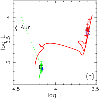
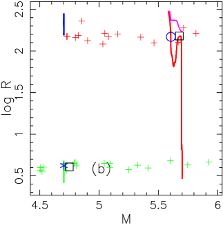
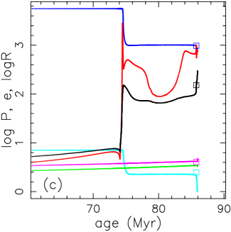
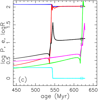
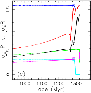
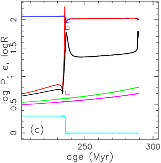
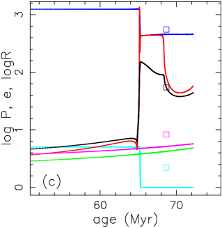
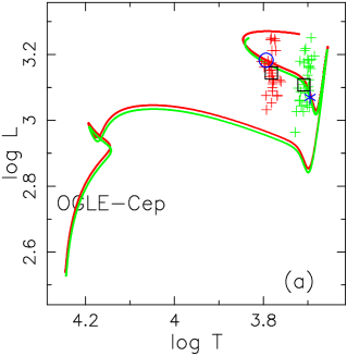
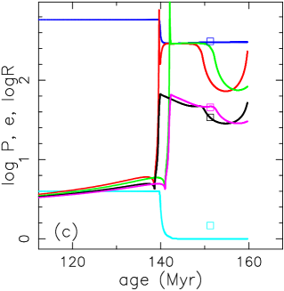
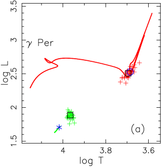
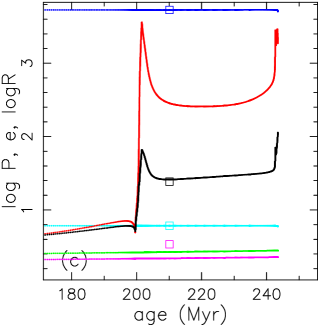
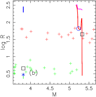
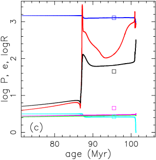
In the case of Aur (Fig. 1), the observational uncertainties in radius, temperature and luminosity are too large to exclude definitely four out of five possible solutions. The primary in the model is almost exactly at the observed radius for the temporary maximum at helium ignition. It will be very near the observed radius just before and just after helium ignition; it then returns to that same radius on the asymptotic giant branch after a truncated ‘blue loop’, and it will in fact pass through the same radius three times as it climbs the asymptotic giant branch. It might have been possible to break the degeneracy by appealing to the circularity (or otherwise) of the orbit. The eccentricity of 0.4 of Aur’s orbit might suggest that there has not yet been much tidal interaction, but panel (c) shows that if the system commenced with , tidal friction would wear it down to 0.4 during helium ignition, after which it would remain fairly constant for a substantial time until the primary returned to about the same radius as in its earlier local maximum.
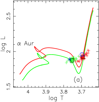
The model of Aur (Capella; Fig. 1) seems to fit the observations very well, but there are inconsistencies in the latter. Two recent published measurements of (the RV amplitude of the secondary) appear quite precise according to their respective internal standard deviations, but the values differ from one other by many : (Torres et al., 2009), or (Weber & Strassmeier, 2011), equivalent to differences of 6 or 24 , respectively. In fact our models for Capella fit much better the values of Weber & Strassmeier. Recently Torres et al. (2015) have revised their to , in good agreement with Weber & Strassmeier (and our theoretical model).
For both binaries, the models include a certain amount of mass loss by way of
stellar wind, as indicated by the middle panels of Fig. 1. Three
types of mass loss are modelled:
(1) In the very reasonable expectation that
all stars, whether single or in a widish binary, with a mass less than
M⊙ end up as white dwarfs, we impose
a rate (referred to as ‘Single Red-Giant Wind’)
which is assumed to be (a) proportional to the ratio of the luminosity to the
binding energy of the envelope, and (b) of sufficient strength to reduce a
non-rotating single 4 M⊙ star to a white dwarf of 1 M⊙,
(2) a
Dynamo-Driven Wind (Eggleton, 2001, 2006), which is included
through a formulation that gives, inter alia, the mass-loss rate as a
function of rotation rate, luminosity, radius and mass (see § 3.2), and
(3) a
mass-loss rate that has been determined empirically by de Jager et al. (1988)
for luminous stars ( ), though it only applies to one or two
of our sample.
For Aur the modelled mass loss is mainly by single red-giant wind, while for Aur it is mainly by dynamo-driven wind, though in neither case is the rate high enough to affect very strongly the agreement with observation. The agreement is actually somewhat better with dynamo-driven wind than without it, but it is difficult to establish that in the face of the uncertainties in the observational data. It may also be worth mentioning that the chromospheric material of Aur (as isolated near to occultation of the hot star at eclipse phases) is rather tightly confined, somewhat suggestive of a magnetic-loop formation (Dr R. E. M. Griffin, p.c.). Furthermore, a few of the systems in the sample show a marked mass anomaly in the sense that the primary is less massive than the secondary, and that could only realistically result from some level of dynamo-driven wind.
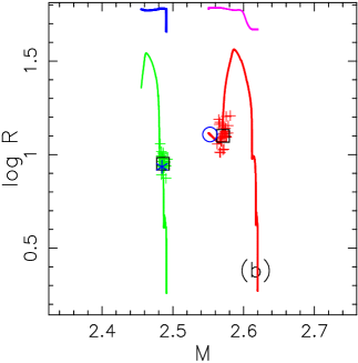
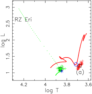
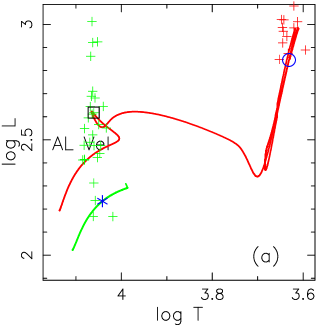
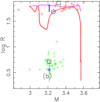
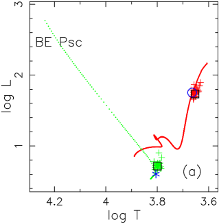
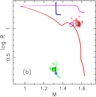
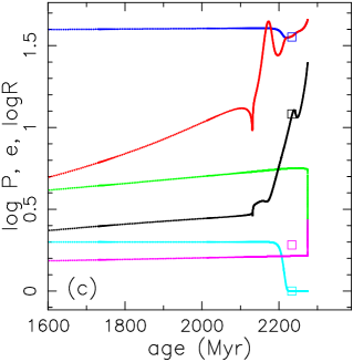
Of the three systems illustrated in Fig. 2, it seems very likely that some kind of mass loss has played a role in RZ Eri, though it is less clear for AL Vel and BE Psc. Several other systems, such as RU Cnc and AS-010538, reveal either substantially more or substantially less mass loss than the Dynamo-Driven Wind model predicts. We discuss these systems more fully in §5.2.
There are several red-giant+main-sequence binaries which are semi-detached. They have not been included in the sample, as most are of fairly short period and we have set a limit at 8 d. Longer-period ones such as SS Lep ( = 250 d; Blind et al., 2011) are symbiotic binaries, and have parameters that are potentially interesting, but they present complications which render precise analyses difficult; they have also been excluded from our sample.
 |
 |
 |
 |
 |
 |
 |
 |
 |
3 Features of The Theoretical Model
Certain elements of a stellar evolution code can be regarded as fairly
standard; they include the equation of state, the nuclear reaction network,
hydrostatic equilibrium, and the radiative opacity (though see below).
However, other elements can vary significantly from one code to another because
a soundly-based physical model is not available. That is true for
(i)
convection, with the mixing-length theory being normal but not necessarily
accurate,
(ii) semi-convective mixing – the formulation adopted here is a
very simple diffusive approximation (Eggleton, 1972),
(iii) convective
core overshooting,
(iv) stellar-wind mass loss, including wind that is driven
by dynamo action owing to rapid rotation, as in RS CVn stars, and other
mass-loss mechanisms that would reduce a single red giant to a white dwarf as
it is evolved towards the top of the asymptotic giant branch by Single Red
Giant Wind
(v) tidal friction, that compels giants in binaries to rotate
much more rapidly than if they were single, and which also tends to circularise
orbits that were initially eccentric,
(vi) rotationally-driven mixing,
and
(vii) diffusive separation of abundances.
The code used here does not incorporate elements (vi) and (vii), mainly because it is conjectured that they will not be very important for the long-term evolution of the stars in the sample. There is no doubt that the surfaces of certain A or F stars can be affected by diffusive separation, leading to Ap, Am and Fm abundance anomalies, but the diffusion is believed to be confined to near-surface layers and is rapidly reversed once a star crosses enough of the Hertzsprung gap for the outer few per cent by mass to be mixed more deeply (as in the case of o Leo, §4.2). Where diffusive separation might make a difference in the long term is in stars of about 1 M⊙, where nuclear evolution is sufficiently slow that diffusion might separate helium and hydrogen significantly in the deep interior. However, very few of the components considered here have masses 1.5 M⊙. Rotationally-driven mixing has been proposed for early type stars, but Tkachenko et al. (2014) found no evidence for it in a detailed abundance analysis of V380 Cyg (§4.2).
The code used here adopts the opacities of Rogers & Iglesias (1992). Asplund et al. (2000, 2005) have suggested that, on the basis of 3-D modelling of the Sun’s convective zone and photosphere, the solar metallicity is somewhat less than the previously standard value of , but – as maintained by Basu & Antia (2006) – it has so far proved hard to reconcile that claim with the previous good agreement between helioseismological results based on the ‘standard’ metallicity (e.g. Christiansen-Dalsgaard & Däppen, 1992). In the meantime we are continuing to use the standard metallicity.
We use an implicitly adaptive mesh-point distribution (Eggleton 1971) which allows us to model stars with no more than 200 meshpoints in them, from centre to photosphere, even with double shell burning. This economy is counterbalanced by the fact that we choose to solve 44 difference equations simultaneously. For example, we solve Clairault’s equation (a second-order DE) for the distortion of each component along with two other first-order DEs that determine the tidal velocity field and the rate of its dissipation by turbulent convective viscosity. The code runs easily on an Apple Mac Pro (reconfigured for Linux, with a Fortran compiler), and takes between 10 minutes and about an hour to solve each of the 60 systems.
The following subsections discuss, in turn, convective core overshooting, wind mass loss, and tidal friction.
3.1 Core Convective Overshooting
The model for core convective overshooting, based here on that proposed by Eggleton (2006), assumes that mixing in the core goes beyond the Schwarzschild boundary () to a boundary . The functional form of may ultimately be determined by 3-D numerical simulations, but more than mesh-points will be necessary and such refinement has probably not yet been reached. It is to be hoped that the 1-D modelling presented here places some restrictions on . In particular, the models for TZ For, SU Cyg, V380 Cyg and Ori, which have primary masses of 2, 6, 13 and 24 M⊙, respectively, show that a modest amount of overshooting must operate between 2 and 6 M⊙ but that by 13 M⊙ the amount (measured in pressure scale-heights, PSH) must be trebled, and even quadrupled by 24 M⊙. The functional form used is given in Appendix A; its effect is to create mixing over an extra 0.16–0.2 PSH in stars with masses 4 M⊙, and over 0.5–0.7 PSH for masses of about 10–13 M⊙; the region affected may in fact extend to 1 PSH by 40 M⊙, but that condition has not yet been tested. It should be noted that the model described and used here differs a little from those used in earlier versions of the same code (e.g., by Pols et al. 1997) by including modestly more core convective overshooting for lower masses, and substantially more for higher masses (as in V380 Cyg and Ori).
 |
 |
 |
 |
 |
 |
 |
 |
 |
TZ For is critical to this discussion because it seems clear that the primary star () must have passed through non-degenerate helium ignition. That would explain its circular 76-d orbit despite the fact that is less than 20% of its Roche-lobe radius. Without overshooting, for masses below 2.5 M⊙ the helium ignition would be a degenerate He flash, requiring to reach a much bigger radius and hence undergo substantial Roche-lobe overflow. If the red giant in TZ For were on the first giant branch, it would not yet be large enough to circularize the orbit; however, if it is in the GK-giant clump it must have undergone non-degenerate helium ignition at a modest radius that was two or three times larger than its present one (8.5 R⊙) but smaller than its Roche-lobe one (45 R⊙). DQ Leo, Equ and And reveal similar evidence, having only slightly different masses and period, and circular orbits.
Primaries in the GK-giant clump that are more massive than about 2.5 M⊙ are not quite so informative, because they would undergo non-degenerate helium ignition either with or without overshooting. They may nevertheless present more information about tidal friction (§3.2). A star in the GK-giant clump with a mass of about 6 M⊙ starts to evolve towards the blue and into the blue loop, where it may be conspicuous as a Cepheid. Reconciling theoretical Cepheid blue loops with observation was a problem for a long time, but was largely resolved by incorporating overshooting into the models (Schröder et al., 1997).
| n | age | ||||||||
| Gyr | M⊙ | d | R⊙ | L⊙ | M⊙/yr | Gauss | |||
| 3 | 0.000 | 1.0242 | 36.71 | 1.019 | 1.519 | 15.1 | 1.70 | Arbitrary starting point on the Hayashi track | |
| 1004 | 0.042 | 1.0129 | 2.991 | -0.050 | -0.137 | 20.8 | 2.65 | Minimum radius, at ZAMS | |
| 1110 | 0.278 | 1.0044 | 6.731 | -0.045 | -0.125 | 14.5 | 3.21 | Rotation slowed, mass loss much down | |
| 1202 | 4.567 | 0.9999 | 24.89 | 0.000 | 0.005 | 1.29 | 11.3 | Present day | |
| 1400 | 10.30 | 0.9970 | 47.38 | 0.166 | 0.307 | 0.35 | 0.35 | Hertzsprung gap | |
| 2200 | 11.77 | 0.9861 | 2949 | 0.887 | 1.384 | 0.0 | 0.0 | Lower first giant branch | |
| 2360 | 11.87 | 0.9379 | - | 1.523 | 2.362 | - | - | Single red-giant wind becoming significant | |
| 2566 | 11.88 | 0.6224 | - | 2.367 | 3.405 | - | - | He flash | |
| 2567 | 11.88 | 0.6207 | - | 1.027 | 1.705 | - | - | ‘Zero Age’ Horizontal Branch | |
| 2976 | 11.97 | 0.6146 | - | 0.924 | 1.634 | - | - | Local minimum radius | |
| 3809 | 12.04 | 0.5525 | - | 1.934 | 3.388 | - | - | Tip of AGB. |
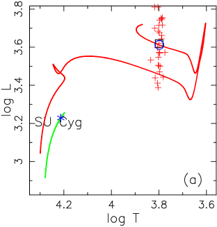
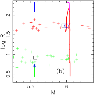
Masses for Cepheids have rarely been obtained directly from double-lined eclipsing (or interferometric) orbits. However one such system in the LMC, OGLE-Cep (see Table 3), has been found to have parameters of 4.165 + 4.134 M⊙, 309.4 d, = 0.166 (Pilecki et al., 2013). The system can be fitted very easily by a theoretical model (Fig. 3), but it needs to use a metallicity that is substantially less than solar. An increase in metallicity tends to reduce the size of blue loops rather drastically. At solar metallicity, blue loops large enough to produce Cepheids are confined to masses greater than 5.5 M⊙, but it also depends on the degree of assumed overshooting; too much shrinks the blue loop to insignificance. We estimate that overshooting at 6 M⊙, roughly the mass of the double-lined but non-eclipsing Cepheid SU Cyg (Evans & Bolton, 1990), must be not much more than at 2 M⊙ (as in TZ For).
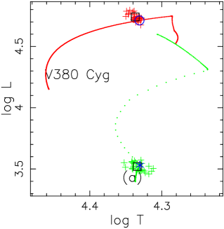
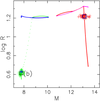
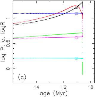
It is interesting to note that the companion to SU Cyg is itself a fairly compact sub-binary of period 4.65 d. Fig. 3 models the SU Cyg system with a fictitious secondary component () that has the same mass as the sub-binary. The primary develops a blue loop that gets it to the location of the Cepheid, though at higher masses still (as in V380 Cyg) it is necessary to include substantially greater overshooting. However, both those Cepheids present a problem, inasmuch as both have eccentric orbits and yet both should have circularized their orbits (according to our models) during the helium ignition stage when the components were larger by a factor of two or more. This is discussed further in §5.3.
V380 Cyg is not an obvious candidate for the present study, since although , at B1.5 III, is technically a giant, it is very much bluer than almost all the other giants. We would argue that must be still within the main sequence band, because if it were in the Hertzsprung gap it would be evolving very rapidly, on a timescale of 100 yr. By contrast, if it is still in the main sequence band (Fig. 3) its evolutionary timescale is more like yr. This system’s relevance to overshooting has been discussed by several authors, including Pietrzyński et al. (2009). Also Ori is an atypical addition: it has an O9.5 II primary, which nevertheless must (we think) be still in the MS band for the same reason.
3.2 Dynamo-Driven Wind and Single Red Giant Wind
As mentioned above, stellar wind mass loss may be regarded as a combination of three contributions. Probably the most significant one for the stars in our sample is dynamo-driven wind, a model for which is discussed in some detail by Eggleton (2001, 2006). From an input of mass, radius, luminosity and stellar rotation period this model produces estimates for (a) the differential rotation rate between the convective envelope and the radiative core, (b) the star-spot cycle time (e.g., 22 years for the Sun), (c) the overall poloidal magnetic field, (d) the mass-loss rate (assuming that the mass loss is driven by destruction of the toroidal field at and above the surface of the star), and (e) the Alfvén radius of the wind as determined by the poloidal field and the wind strength. The rotation rate will modify itself in the course of time through magnetic braking, whereby angular momentum is transferred to the wind; the latter is assumed to be rotating rigidly out to the Alfvén radius and then escaping freely. This process works for single stars as well as stars in binaries, though in single stars it is self-limiting because the dynamo weakens as the star spins down, whereas in binary stars that are close enough it can be self-amplifying, since tidal friction may reduce the separation and therefore the spin rate increases as the star loses angular momentum to the wind.
Table 2 gives a few stages in the evolution of a single star that resembles the Sun at 4.567 Gyr. It tabulates the rotational period, the mass-loss rate, the poloidal magnetic field and the Alfvén radius. The Table suggests that a dynamo-driven wind is only responsible for significant mass loss in roughly the first 300 Myr; most occurs in just the first 150 Myr, by which time the rotation has slowed to about 5 d from a peak value of 3 d. Subsequent mass loss, producing a white-dwarf precursor of 0.55 M⊙, is modelled by a ‘Reimers-like’ wind (Reimers, 1975), where is proportional to the ratio of luminosity to the binding energy of the envelope above the burning shell, as described in §2 above and referred to as a ‘single red-giant wind’.
Mass loss through a dynamo-driven wind affects all of our theoretical models in principle, but in the great majority it makes rather little difference. The three systems represented in Fig. 2 display a range of disparity in the inferred rates of mass loss ranging from about 20 times more than is predicted for RZ Eri to 3 times less than predicted for BE Psc. For AL Vel the predicted amount of mass loss appears to match what can be inferred from observation to within a factor of 2. In HR 6046 (online only) the theoretical mass loss exceeds what is probably required by a factor of about 10.
Several (11) of our 60 systems come into substantial conflict with our mass-loss algorithms. We discuss these individually in §4.2 and collectively in §5.2.
3.3 Tidal Friction.
The model of tidal friction used here has been described in some detail by Eggleton (2006), and in a somewhat preliminary version by Eggleton et al. (1999). It relies on turbulent convective motion as the dissipatory agent for tidal motion. For the most part it seems to be effective at circularizing orbits that are known to be circular now, but which are wide enough that they were very probably eccentric at age zero – as in the case of Aur (Fig. 1). In that system the primary is about 8 times smaller than its Roche lobe, and tidal friction is unlikely to have circularized its orbit unless its radius were about 3 times its present size at helium ignition (based on a comparison with double-main-sequence binaries). In Aur (Fig. 1) the orbit, still eccentric ( 0.4), can be modelled satisfactorily by adopting an initial = 0.85; the model suggests that it became partly circularized during helium ignition, fell to its present level, and will drop fairly rapidly in the future.
Only 4 systems come into substantial conflict with our tidal-friction model. We discuss these in §5.3.
 |
 |
 |
 |
 |
 |
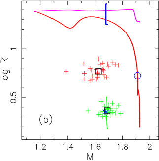
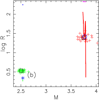
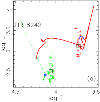
3.4 ‘Over-Evolved Secondaries’
Fig. 4 shows our attempts to model Per (upper set) and HR 8242 (lower set). In both systems the secondary appears to have evolved considerably more than it could have done in the time that the primary took to reach something like its present radius. The observed mass ratio is about 1.5 in both cases and the secondary should have barely left the ZAMS, but in fact it has evolved to something like twice its ZAMS radius. One explanation could be that the binary was formed by a capture process between an older star and a younger star, but it seems very unlikely that this occurred in two out of 60 systems. A different, and possibly more tenable, explanation is offered in §5.1.
4 Individual Cases
4.1 Presenting the information
The sample of 60 systems was listed in Table 1, together with some aliases and the primary literature references. Table 3 records what has been found in the literature about each system from radial velocity measurements of both components, from modelling the photometry and spectroscopy, and from astrometry. For each system ten or eleven more-or-less directly measured quantities, which we refer to as ‘raw’, are listed on the first line, with their measurement uncertainties on the second line. The quantities range from orbital radial velocity amplitudes to parallax, for each system. The eleventh measurable quantity, inclination, is of course not available unless the system is either eclipsing or astrometric. These quantities are transformed by a standard procedure (Appendix B) into quantities which we refer to as ‘derived’ – mass, temperature, radius and luminosity, for each component – that are easily compared with the theoretical models, and that are are listed in Table 4. Each system is illustrated by a plot consisting of three panels, as for the 10 systems in Figs 1 – 4. The 50 not shown here are accessible online.
Since a spectral type is a visual description of a spectrum rather than a measurement of it, and since the isolated spectrum of the primary cannot be seen in most of these binaries, there is unavoidably some degree of subjectivity attached to the spectral types listed in Table 3. The spectral type of the primary is usually deemed to be that of the standard which was adopted as its surrogate in the subtraction procedure to uncover the secondary spectrum, though not infrequently (particularly for the brighter giants) the match can be less than ideal. For the secondary, the individualities of available single, and preferably low-rotating, standard early-type spectra present a different challenge and may be circumnavigated by fitting a synthetic spectrum to the extracted (supposedly pure) version of its spectrum which then has to be translated into a spectral type, often (also somewhat subjectively) via its () as tabulated by (for instance) Schmidt-Kaler (1982). The spectral types listed in Table 3 are therefore guides rather than accurate statements.
The tabulated parallaxes are mostly either the re-worked Hipparcos values (van Leeuwen, 2007) or else from Gaia (Gaia Collaboration et al., 2016; Lindegren et al., 2016); but in principle a system that is both eclipsing and double-lined can provide a parallax independent of astrometry, as for several LMC and SMC systems. It should be noted that a system with an orbital period of order one year may have an inherently ambiguous astrometric parallax as a result of the confusion of the target’s orbit and its parallactic motion.
The data compiled in Table 3 consists of 10 or 11 observationally determined numbers per system. Many systems have an observed inclination, as determined by either an eclipse or an astrometric orbit or both, but several do not, and we then estimate an inclination by matching the system to theoretical systems. In Table 3 an E (39), A (13) or N (10) in the last column means Eclipsing, Astrometric or Neither. Two are both E and A.
| No. | Name | plx | Type | ||||||||||
|---|---|---|---|---|---|---|---|---|---|---|---|---|---|
| spectra | day | km/s | km/s | mas | GoF | ||||||||
| Z | |||||||||||||
| 1 | SMC-130 | 120.470 | 0.000 | 33.42 | 32.54 | 16.783 | -0.72 | 0.24 | 4515 | 4912 | 0.0162 | 83.09 | E |
| G7III | 0.001 | 0.000 | 0.12 | 0.11 | 0.010 | 0.10 | 0.02 | 150 | 150 | 0.0008 | 0.10 | 1.08 | |
| + K1III | 120.470 | 0.000 | 33.42 | 32.54 | 16.783 | -0.95 | 0.24 | 4365 | 4812 | 0.0180 | 83.09 | .004 | |
| 2 | SMC-126 | 635.000 | 0.042 | 18.48 | 18.54 | 16.771 | -0.192 | 0.24 | 4480 | 4510 | 0.0160 | 86.92 | E |
| K2III | 0.009 | 0.002 | 0.110 | 0.10 | 0.01 | 0.020 | 0.02 | 150 | 150 | 0.0030 | 0.09 | 0.92 | |
| + K1III | 635.000 | 0.042 | 18.48 | 18.54 | 16.771 | -0.222 | 0.24 | 4250 | 4350 | 0.0165 | 86.92 | .004 | |
| 3 | SMC-101 | 102.900 | 0.000 | 39.44 | 41.03 | 17.177 | -0.203 | 0.20 | 5170 | 5580 | 0.0154 | 88.04 | E |
| K2III | 0.000 | 0.000 | 0.20 | 0.12 | 0.010 | 0.020 | 0.02 | 95 | 90 | 0.0003 | 0.23 | 1.05 | |
| + K1II | 102.900 | 0.000 | 39.44 | 41.03 | 17.177 | -0.203 | 0.20 | 5170 | 5280 | 0.0154 | 88.04 | .004 | |
| 4 | HD 4615 | 302.771 | 0.435 | 27.52 | 30.8 | 6.82 | -1.10 | 0.25 | 4400 | 8700 | 2.48 | 71.4 | N |
| K2III | 0.020 | 0.003 | 0.10 | 0.9 | 0.02 | 0.20 | 0.05 | 200 | 500 | 0.59 | 2.0 | 0.17 | |
| + A2V | 302.771 | 0.435 | 27.52 | 30.8 | 6.82 | -1.10 | 0.25 | 4400 | 8500 | 2.68 | 71.4 | .02 | |
| 5 | And | 115.73 | 0.003 | 17.98 | 19.03 | 4.40 | -0.54 | 0.05 | 5050 | 5000 | 13.3 | 30.5 | A |
| G8III | 0.02 | 0.002 | 0.09 | 0.11 | 0.02 | 0.02 | 0.01 | 200 | 200 | 0.5 | 0.20 | 0.40 | |
| + G8III | 115.73 | 0.003 | 18.04 | 18.92 | 4.40 | -0.54 | 0.05 | 5000 | 5050 | 13.3 | 30.5 | .02 | |
| 6 | SMC-108 | 185.220 | 0.000 | 37.85 | 37.96 | 15.205 | 0.081 | 0.28 | 4955 | 5675 | 0.01562 | 78.87 | E |
| F9II + G7II | 0.002 | 0.000 | 0.08 | 0.09 | 0.01 | 0.02 | 0.02 | 105 | 90 | 0.00030 | 0.10 | 0.00 | |
| + G7III | 185.220 | 0.000 | 37.85 | 37.96 | 15.205 | 0.081 | 0.28 | 4955 | 5675 | 0.01562 | 78.87 | .004 | |
| 7 | BE Psc | 35.670 | 0.000 | 41.52 | 49.43 | 8.76 | -1.95 | 0.80 | 4500 | 6300 | 3.8 | 81.8 | E |
| K1III | 0.000 | 0.000 | 0.19 | 0.41 | 0.02 | 0.05 | 0.02 | 70 | 100 | 0.2 | 0.1 | 1.05 | |
| + F6IV-V | 35.670 | 0.000 | 41.52 | 49.24 | 8.76 | -2.25 | 0.80 | 4550 | 6350 | 3.8 | 81.8 | .02 | |
| 8 | ASAS–010538 | 8.069 | 0.000 | 73.0 | 75.74 | 10.1 | -0.75 | 0.19 | 4889 | 6156 | 2.66 | 79.90 | E |
| 0.000 | 0.000 | 1.3 | 0.26 | 0.2 | 0.05 | 0.02 | 98 | 176 | 0.23 | 0.65 | 0.45 | ||
| 8.069 | 0.000 | 73.0 | 75.74 | 10.1 | -0.75 | 0.19 | 4889 | 6156 | 2.35 | 79.90 | .02 | ||
| 9 | AI Phe | 24.590 | 0.188 | 49.24 | 50.90 | 8.58 | 0.22 | 0.01 | 5010 | 6310 | 5.94 | 88.45 | E |
| K0IV | 0.000 | 0.000 | 0.10 | 0.10 | 0.02 | 0.25 | 0.05 | 250 | 300 | 0.24 | 1.00 | 0.64 | |
| + F7V | 24.590 | 0.188 | 49.24 | 50.90 | 8.58 | -0.22 | 0.01 | 4910 | 6110 | 5.78 | 88.45 | .01 | |
| 10 | Per | 1515.880 | 0.734 | 19.09 | 23.0 | 3.93 | -1.71 | 0.00 | 5050 | 8000 | 12.83 | 85 | EA |
| G8IIIa | 0.100 | 0.007 | 0.35 | 4.0 | 0.02 | 0.10 | 0.05 | 150 | 300 | .36 | 2 | 0.89 | |
| + A6V | 1515.880 | 0.734 | 19.09 | 23.3 | 3.93 | -1.81 | 0.00 | 4950 | 8100 | 13.70 | 85 | .01 | |
| 11 | Per | 5327.7 | 0.785 | 14.53 | 21.73 | 2.91 | -1.33 | 0.00 | 4950 | 9250 | 13.41 | 90 | EA |
| G8IIIa | 0.6 | 0.002 | 0.10 | 0.20 | 0.02 | 0.10 | 0.05 | 200 | 200 | 0.51 | 2.00 | – | |
| + A2IV | 5327.7 | 0.785 | 14.53 | 21.73 | 2.91 | -1.33 | 0.00 | 4950 | 9250 | 13.41 | 90.00 | .02 | |
| 12 | TZ For | 75.770 | 0.000 | 38.81 | 40.80 | 6.89 | -0.25 | 0.17 | 4950 | 6350 | 5.44 | 85.6 | E |
| G8III | 0.000 | 0.010 | 0.01 | 0.02 | 0.02 | 0.10 | 0.05 | 200 | 250 | 0.25 | 0.05 | 0.57 | |
| + F7III | 75.666 | 0.000 | 38.81 | 40.80 | 6.89 | -0.25 | 0.17 | 4900 | 6550 | 5.75 | 85.6 | .03 | |
| 13 | HR 1129 | 6124. | 0.678 | 15.87 | 17.60 | 4.82 | -1.20 | 0.93 | 5250 | 13000 | 3.29 | 87 | A |
| G2Ib-II | 3. | 0.003 | 0.08 | 0.34 | 0.02 | 0.40 | 0.35 | 150 | 500 | 0.27 | 4 | 0.80 | |
| + B7III-IV | 6124. | 0.678 | 15.90 | 17.40 | 4.82 | -1.60 | 0.63 | 5250 | 14000 | 3.20 | 87 | .01 | |
| 14 | OGLE-Cep | 309.400 | 0.166 | 32.14 | 32.38 | 15.32 | -0.310 | 0.50 | 6050 | 5120 | 0.020 | 86.83 | E |
| F7Ib | 0.100 | 0.003 | 0.07 | 0.06 | 0.02 | 0.010 | 0.05 | 160 | 130 | 0.001 | 0.02 | 0.00 | |
| + G4II | 309.400 | 0.166 | 32.14 | 32.38 | 15.32 | -0.310 | 0.50 | 6050 | 5120 | 0.020 | 86.83 | .004 | |
| 15 | RZ Eri | 39.280 | 0.350 | 50.80 | 48.90 | 7.78 | 0.20 | 0.00 | 4800 | 7200 | 5.55 | 89 | E |
| G8-K0III | 0.000 | 0.010 | 0.10 | 1.00 | 0.02 | 0.10 | 0.05 | 200 | 300 | 0.44 | 2 | 0.72 | |
| + A8-F0IV | 39.280 | 0.350 | 50.80 | 48.90 | 7.78 | 0.05 | 0.00 | 5000 | 7000 | 5.00 | 89 | .02 | |
| 16 | OGLE-01866 | 251.007 | 0.241 | 33.28 | 33.27 | 16.12 | -0.074 | 0.345 | 4541 | 5327 | 0.020 | 83.3 | E |
| 0.004 | 0.001 | 0.05 | 0.14 | 0.09 | 0.090 | 0.060 | 81 | 87 | 0.001 | 0.10 | 0.00 | ||
| 251.007 | 0.241 | 33.28 | 33.27 | 16.12 | -0.074 | 0.345 | 4541 | 5050 | 0.020 | 83.3 | .004 | ||
| 17 | OGLE-03160 | 150.020 | 0.000 | 30.35 | 30.47 | 17.4 | -1.136 | 0.37 | 4490 | 4954 | 0.0199 | 83.36 | E |
| 0.001 | 0.001 | 0.11 | 0.14 | 0.09 | 0.090 | 0.09 | 77 | 72 | 0.0010 | 0.57 | 0.00 | ||
| 150.020 | 0.000 | 30.35 | 30.47 | 17.4 | -1.136 | 0.37 | 4490 | 4954 | 0.0199 | 83.36 | .004 | ||
| 18 | Aur | 972.150 | 0.393 | 23.26 | 27.80 | 3.69 | -2.11 | 0.25 | 3960 | 15200 | 4.15 | 90 | E |
| K4Ib | 0.060 | 0.005 | 0.15 | 2.80 | 0.02 | 0.10 | 0.05 | 100 | 200 | 0.29 | 2.00 | 0.49 | |
| + B6V | 972.150 | 0.393 | 23.26 | 27.60 | 3.69 | -2.11 | 0.25 | 3960 | 14900 | 4.25 | 90 | .02 | |
| 19 | OGLE-06575 | 189.822 | 0.000 | 37.72 | 36.03 | 15.712 | -0.152 | 0.32 | 4681 | 4903 | 0.020 | 82.06 | E |
| 0.002 | 0.000 | 0.07 | 0.09 | 0.090 | 0.090 | 0.09 | 77 | 72 | 0.001 | 0.13 | 0.00 | ||
| 189.822 | 0.000 | 37.72 | 36.03 | 15.712 | -0.152 | 0.32 | 4681 | 4903 | 0.020 | 82.06 | .004 | ||
| 20 | OGLE-EB | 214.400 | 0.040 | 32.65 | 33.67 | 16.2 | -0.44 | 0.01 | 5288 | 5470 | 0.020 | 88.2 | E |
| K4III | 0.001 | 0.010 | 0.08 | 0.10 | 0.02 | 0.10 | 0.05 | 81 | 96 | 0.001 | 0.1 | 0.00 | |
| + K4III | 214.171 | 0.039 | 32.76 | 33.37 | 16.2 | -0.44 | 0.01 | 5288 | 5470 | 0.020 | 88.2 | .004 | |
| 21 | OGLE-09660 | 167.635 | 0.052 | 35.13 | 34.91 | 16.27 | -0.504 | 0.38 | 5352 | 4677 | 0.020 | 87.8 | E |
| 0.001 | 0.001 | 0.08 | 0.16 | 0.090 | 0.090 | 0.01 | 99 | 99 | 0.002 | 0.3 | 0.81 | ||
| 167.635 | 0.052 | 35.13 | 34.91 | 16.27 | -0.504 | 0.38 | 5152 | 4677 | 0.023 | 87.8 | .004 | ||
| 22 | OGLE-10567 | 117.871 | 0.000 | 39.31 | 41.32 | 16.48 | -0.26 | 0.30 | 5067 | 4704 | 0.020 | 83.4 | E |
| 0.001 | 0.000 | 0.14 | 0.13 | 0.09 | 0.09 | 0.09 | 80 | 73 | 0.001 | 0.3 | 0.00 | ||
| 117.871 | 0.000 | 39.31 | 41.32 | 16.48 | -0.26 | 0.30 | 5067 | 4704 | 0.020 | 83.4 | .004 | ||
| 23 | OGLE-26122 | 771.781 | 0.419 | 23.8 | 25.08 | 16.63 | -0.76 | 0.42 | 4989 | 4995 | 0.020 | 88.45 | E |
| 0.005 | 0.002 | 0.1 | 0.14 | 0.09 | 0.01 | 0.01 | 99.9 | 99.9 | 0.001 | 0.04 | 0.00 | ||
| 771.781 | 0.419 | 23.8 | 25.08 | 16.63 | -0.76 | 0.42 | 4989 | 4995 | 0.020 | 88.45 | .004 | ||
| 24 | Aur | 104.000 | 0.001 | 25.96 | 26.840 | 0.08 | 0.13 | 0.01 | 4920 | 5680 | 76.19 | 137.2 | A |
| G9III | 0.000 | 0.001 | 0.00 | 0.024 | 0.01 | 0.10 | 0.01 | 196.8 | 230 | 0.47 | 0.05 | 0.54 | |
| + G0III | 104.000 | 0.000 | 25.96 | 26.840 | 0.08 | 0.23 | 0.01 | 4920 | 5900 | 76.19 | 137.2 | .02 | |
| 25 | OGLE-15260 | 157.324 | 0.000 | 27.93 | 27.67 | 17 | -0.676 | 0.30 | 4320 | 4706 | 0.0199 | 82.9 | E |
| 0.001 | 0.000 | 0.14 | 0.11 | 0.09 | 0.090 | 0.09 | 81 | 87 | 0.0010 | 0.3 | 0.00 | ||
| 157.324 | 0.000 | 27.93 | 27.67 | 17 | -0.676 | 0.30 | 4320 | 4706 | 0.0199 | 82.9 | .004 | ||
| 26 | Ori | 5.732 | 0.112 | 104.6 | 266.0 | 2.41 | -3.00 | 0.15 | 30000 | 24000 | 2.9 | 76.4 | E |
| O9.5II | 0.001 | 0.010 | 1.6 | 20.0 | 0.02 | 0.40 | 0.05 | 1000 | 1000 | 0.5 | 0.2 | 0.25 | |
| + B0V | 5.732 | 0.112 | 104.6 | 266.0 | 2.41 | -3.20 | 0.15 | 30500 | 23700 | 2.8 | 76.4 | .02 | |
| 27 | HR 2030 | 66.452 | 0.017 | 25.98 | 25.6 | 5.96 | -0.20 | 0.40 | 4550 | 11750 | 2.91 | 29.5 | N |
| K0IIb | 0.001 | 0.005 | 0.15 | 2.8 | 0.02 | 0.10 | 0.05 | 150 | 250 | 0.67 | 1.0 | 0.00 | |
| + B8IV | 66.452 | 0.017 | 25.98 | 25.6 | 5.96 | -0.20 | 0.40 | 4550 | 11750 | 2.91 | 29.5 | .02 | |
| 28 | V415 Car | 195.300 | 0.000 | 24.29 | 38.6 | 4.41 | -3.20 | 0.00 | 4981 | 9388 | 5.99 | 82.7 | E |
| G6II | 0.000 | 0.010 | 0.10 | 1.0 | 0.02 | 0.20 | 0.05 | 199.2 | 375.5 | 0.18 | 2.0 | 0.43 | |
| + A1V | 195.300 | 0.000 | 24.29 | 38.6 | 4.41 | -3.20 | 0.00 | 4750 | 9650 | 5.99 | 82.7 | .01 | |
| 29 | HR 3222 | 955.130 | 0.327 | 14.06 | 16.85 | 6.03 | -1.92 | 0.00 | 4840 | 7000 | 6.78 | 61.5 | N |
| K0III | 0.130 | 0.003 | 0.04 | 0.38 | 0.02 | 0.10 | 0.05 | 150 | 300 | 0.45 | 4.0 | 0.18 | |
| + kA8hF2mF4 | 955.130 | 0.327 | 14.06 | 16.85 | 6.03 | -1.92 | 0.00 | 4800 | 7150 | 6.78 | 61.5 | .02 | |
| 30 | AL Vel | 96.11 | 0.000 | 42.60 | 44.0 | 8.65 | -1.27 | 0.65 | 4300 | 11500 | 1.18 | 85.3 | E |
| K1II-III | 0.00 | 0.010 | 0.10 | 1.0 | 0.02 | 0.10 | 0.05 | 172 | 460 | 0.31 | 2.0 | 0.71 | |
| + B8V: | 96.11 | 0.000 | 42.60 | 44.0 | 8.65 | -1.27 | 0.55 | 4300 | 11100 | 1.00 | 85.3 | .02 |
| No. | Name | plx | Type | ||||||||||
|---|---|---|---|---|---|---|---|---|---|---|---|---|---|
| spectra | day | km/s | km/s | mas | GoF | ||||||||
| Z | |||||||||||||
| 31 | RU Cnc | 10.170 | 0.000 | 70.46 | 67.5 | 10.1 | -0.30 | 0.28 | 4800 | 6400 | 2.64 | 90 | E |
| K1IV | 0.000 | 0.010 | 0.10 | 1.0 | 0.02 | 0.10 | 0.05 | 200 | 250 | 0.25 | 2 | 0.59 | |
| + F5 | 10.170 | 0.000 | 70.46 | 67.5 | 10.1 | -0.30 | 0.35 | 5000 | 6300 | 2.80 | 90 | .02 | |
| 32 | 45 Cnc | 1009.360 | 0.461 | 20.04 | 20.75 | 5.62 | 0.15 | 0.00 | 5030 | 8500 | 3.52 | 67 | N |
| G8III | 0.120 | 0.002 | 0.06 | 0.23 | 0.02 | 0.10 | 0.05 | 150 | 300 | 0.34 | 2 | 0.86 | |
| + A3III | 1009.340 | 0.461 | 20.03 | 20.55 | 5.62 | 0.12 | 0.00 | 4880 | 9200 | 3.96 | 67 | .02 | |
| 33 | Leo | 14.498 | 0.000 | 54.80 | 62.08 | 3.52 | -0.91 | 0.00 | 6100 | 7600 | 25.03 | 57.6 | A |
| F8IIIm | 0.000 | 0.000 | 0.08 | 0.16 | 0.02 | 0.10 | 0.05 | 200 | 200 | 0.22 | 0.1 | 0.87 | |
| + A7m | 14.498 | 0.000 | 54.75 | 61.95 | 3.52 | -0.91 | 0.04 | 6100 | 7600 | 24.5 | 57.7 | .02 | |
| 34 | DQ Leo | 71.691 | 0.000 | 30.12 | 33.0 | 4.5 | -0.44 | 0.00 | 5300 | 7800 | 14.02 | 50.1 | A |
| G7III | 0.000 | 0.010 | 0.07 | 1.4 | 0.02 | 0.10 | 0.05 | 200 | 200 | 0.23 | 0.5 | 1.00 | |
| + A7IV | 71.691 | 0.000 | 30.12 | 33.0 | 4.5 | -0.44 | 0.00 | 5000 | 7700 | 14.65 | 50.1 | .02 | |
| 35 | 12 Com | 396.411 | 0.598 | 24.40 | 30.6 | 4.80 | -0.50 | 0.00 | 5300 | 8500 | 11.07 | 64 | N |
| G7III | 0.000 | 0.001 | 0.06 | 0.4 | 0.02 | 0.10 | 0.05 | 200 | 500 | 0.24 | 5 | 0.92 | |
| + A3IV | 396.411 | 0.598 | 24.40 | 30.2 | 4.80 | -0.70 | 0.09 | 5300 | 8700 | 11.6 | 64 | 0.02 | |
| 36 | 3 Boo | 36.006 | 0.543 | 52.30 | 59.0 | 5.97 | -0.07 | 0.00 | 5850 | 6750 | 11.15 | 74.5 | N |
| G0IV | 0.000 | 0.002 | 0.19 | 0.6 | 0.02 | 0.10 | 0.05 | 150 | 150 | 0.40 | 2.0 | 1.04 | |
| + F2p | 36.006 | 0.543 | 52.30 | 59.0 | 5.97 | -0.27 | 0.00 | 5550 | 6750 | 11.90 | 74.5 | 0.02 | |
| 37 | HR 5983 | 108.206 | 0.000 | 19.83 | 22.41 | 5.79 | -0.89 | 0.06 | 5070 | 9000 | 4.98 | 33 | N |
| G7IIIa | 0.005 | 0.010 | 0.13 | 0.34 | 0.02 | 0.10 | 0.05 | 150 | 300 | 0.30 | 2 | 0.45 | |
| + A2.5IV | 108.206 | 0.000 | 19.83 | 22.41 | 5.79 | -0.89 | 0.06 | 5000 | 8600 | 4.70 | 33 | 0.02 | |
| 38 | HR 6046 | 2201.00 | 0.68 | 15.51 | 15.69 | 5.63 | -3.00 | 0.00 | 3720 | 4470 | 4.83 | 80 | A |
| K3II | 0.00 | 0.01 | 0.05 | 0.14 | 0.01 | 0.10 | 0.05 | 150 | 180 | .78 | 10 | 0.82 | |
| + K0IV | 2201.00 | 0.68 | 15.51 | 15.69 | 5.63 | -3.10 | 0.01 | 3720 | 4900 | 4.83 | 80 | 0.02 | |
| 39 | ASAS-180057 | 269.496 | 0.000 | 35.38 | 35.11 | 10.327 | -0.037 | 1.60 | 4535 | 4211 | .49 | 88.67 | E |
| K4II | 0.014 | 0.000 | 0.10 | 0.10 | 0.099 | 0.009 | 0.10 | 80 | 80 | .35 | 0.21 | 0.02 | |
| + K1II | 269.496 | 0.000 | 35.38 | 35.11 | 10.327 | -0.037 | 1.60 | 4535 | 4211 | .467 | 88.67 | .02 | |
| 40 | ASAS–182510 | 86.650 | 0.000 | 45.12 | 45.45 | 10.87 | -0.90 | 1.35 | 4800 | 4830 | 0.85 | 85.6 | 1.000 |
| 0.000 | 0.000 | 0.12 | 0.13 | 0.02 | 0.40 | 0.05 | 100 | 107 | 0.25 | 0.8 | 0.74 | ||
| 86.650 | 0.000 | 45.12 | 45.45 | 10.87 | -0.50 | 1.35 | 4650 | 4950 | 0.61 | 85.6 | 1.000 | ||
| 41 | V1980 Sgr | 40.51 | 0.000 | 42.53 | 41.14 | 10.2 | -0.30 | 0.97 | 4783 | 4600 | 1.31 | 84.2 | E |
| 0.00 | 0.000 | 0.59 | 0.57 | 0.0 | 0.10 | 0.00 | 82 | 163 | 0.2 | 1.4 | 1.19 | ||
| 40.51 | 0.000 | 42.53 | 41.14 | 10.2 | -0.30 | 0.97 | 4487 | 4529 | 1.50 | 84.2 | .02 | ||
| 42 | V2291 Oph | 385.0 | 0.311 | 25.30 | 33.1 | 5.64 | -1.78 | 0.60 | 4900 | 11600 | 4.14 | 87 | E |
| G9IIb | 0.2 | 0.008 | 0.22 | 0.5 | 0.02 | 0.10 | 0.05 | 150 | 500 | 0.41 | 2 | 0.35 | |
| + B8.5IV | 385.0 | 0.311 | 25.30 | 33.1 | 5.64 | -1.78 | 0.60 | 4900 | 11100 | 4.34 | 87 | .02 | |
| 43 | 113 Her | 245.325 | 0.101 | 15.48 | 22.58 | 4.57 | -2.30 | 0.00 | 5050 | 9500 | 6.91 | 40.2 | A |
| G7II | 0.006 | 0.005 | 0.09 | 0.30 | 0.02 | 0.10 | 0.05 | 150 | 300 | 0.29 | 0.6 | 0.75 | |
| + A0V | 245.325 | 0.101 | 15.48 | 22.58 | 4.57 | -2.20 | 0.00 | 4850 | 9200 | 7.31 | 39.5 | .02 | |
| 44 | KIC 10001167 | 120.39 | 0.155 | 25.07 | 26.64 | 10.39 | -3.60 | 0.05 | 4000 | 5160 | 1.23 | 87.6 | E |
| 0.00 | 0.002 | 0.10 | 0.85 | 0.09 | 0.09 | 0.05 | 99 | 99 | 0.24 | 0.3 | 1.33 | ||
| 120.39 | 0.155 | 25.07 | 26.64 | 10.39 | -3.70 | 0.05 | 4000 | 5160 | 2.20 | 87.6 | .02 | ||
| 45 | KIC 5786154 | 197.918 | 0.378 | 24.67 | 25.71 | 14.00 | -2.38 | 0.05 | 4350 | 5800 | 0.305 | 89.1 | E |
| 0.001 | 0.001 | 0.02 | 0.08 | 0.09 | 0.09 | 0.05 | 99 | 99 | 0.09 | 0.1 | 1.02 | ||
| 197.918 | 0.378 | 24.67 | 25.71 | 14.00 | -2.38 | 0.05 | 4600 | 5600 | 0.305 | 89.1 | .02 | ||
| 46 | KIC 3955867 | 33.657 | 0.012 | 37.83 | 45.43 | 14.90 | -2.50 | 0.05 | 4200 | 5700 | 3.15 | 86.75 | E |
| 0.000 | 0.001 | 0.20 | 0.02 | 0.09 | 0.09 | 0.09 | 99 | 99 | 0.99 | 0.02 | 1.56 | ||
| 33.657 | 0.012 | 37.83 | 45.43 | 14.90 | -2.50 | 0.05 | 4500 | 5500 | 3.05 | 86.75 | .02 | ||
| 47 | KIC 7037405 | 207.108 | 0.228 | 23.56 | 26.02 | 12.00 | -2.62 | 0.05 | 4500 | 6000 | 0.568 | 89.12 | E |
| 0.000 | 0.001 | 0.01 | 0.25 | 0.09 | 0.09 | 0.05 | 99 | 99 | 0.03 | 0.09 | 1.06 | ||
| 207.108 | 0.228 | 23.56 | 26.02 | 12.00 | -2.92 | 0.05 | 4500 | 6000 | 0.578 | 89.12 | .02 | ||
| 48 | 9 Cyg | 1571.65 | 0.789 | 22.42 | 24.74 | 5.39 | -0.75 | 0.10 | 5050 | 9250 | 5.22 | 117 | A |
| G8IIIa | 0.38 | 0.002 | 0.12 | 0.33 | 0.02 | 0.10 | 0.02 | 200 | 300 | 0.84 | 3 | 0.79 | |
| + A2V | 1571.65 | 0.789 | 22.42 | 24.94 | 5.39 | -0.55 | 0.10 | 4850 | 9250 | 6.00 | 115 | .02 | |
| 49 | SU Cyg | 549.2 | 0.343 | 30.07 | 32.2 | 6.98 | -3.00 | 1.10 | 6300 | 8000 | 1.52 | 85 | A |
| F2Iab | 0.1 | 0.003 | 0.12 | 1.6 | 0.02 | 0.50 | 0.20 | 200 | 500 | 0.27 | 2 | 0.71 | |
| + (B8 + A0:) | 549.2 | 0.343 | 30.07 | 32.2 | 6.98 | -3.00 | 1.10 | 6300 | 8000 | 0.92 | 85 | .01 | |
| 50 | Sge | 3705.0 | 0.451 | 7.89 | 8.9 | 3.68 | -2.50 | 0.06 | 3500 | 10500 | 5.49 | 33.5 | A |
| M2IIab | 3.0 | 0.009 | 0.09 | 2.6 | 0.02 | 0.30 | 0.05 | 200 | 500 | 0.72 | 0.3 | 0.70 | |
| + B9.5V | 3705.0 | 0.451 | 7.89 | 8.7 | 3.68 | -2.00 | 0.06 | 3500 | 10900 | 4.60 | 33.5 | .02 | |
| 51 | V380 Cyg | 12.43 | 0.206 | 95.1 | 160.5 | 5.68 | -3.03 | 0.70 | 21750 | 21600 | .97 | 81.0 | E |
| B1.5III | 0.00 | 0.010 | 0.3 | 1.2 | 0.02 | 0.05 | 0.05 | 280 | 550 | .02 | 0.5 | .00 | |
| + B2V | 12.43 | 0.206 | 95.1 | 160.5 | 5.68 | -3.03 | 0.70 | 21750 | 21600 | .97 | 81.0 | .02 | |
| 52 | HD 187669 | 88.387 | 0.000 | 34.444 | 34.458 | 8.88 | -0.96 | 0.38 | 4330 | 4650 | 1.47 | 87.68 | E |
| K2.5III | 0.001 | 0.001 | 0.015 | 0.015 | 0.01 | 0.05 | 0.05 | 70 | 80 | 0.55 | 0.15 | 0.11 | |
| + K0-0.5III | 88.387 | 0.000 | 34.444 | 34.458 | 8.88 | -0.96 | 0.38 | 4330 | 4650 | 1.65 | 87.68 | .02 | |
| 53 | HD 190585 | 171.277 | 0.356 | 33.19 | 33.53 | 9.65 | -0.15 | 2.20 | 4930 | 4930 | 1.27 | 87.05 | E |
| 0.001 | 0.001 | 0.05 | 0.05 | 0.09 | 0.09 | 0.09 | 199 | 199 | 0.28 | 0.03 | 0.93 | ||
| 171.277 | 0.356 | 33.19 | 33.53 | 9.65 | -0.15 | 2.20 | 4600 | 4600 | 1.77 | 87.05 | .02 | ||
| 54 | HD 190361 | 1512.0 | 0.085 | 9.67 | 14.5 | 7.16 | -1.40 | 0.93 | 3800 | 17000 | 0.75 | 33 | N |
| K4Ib | 1.7 | 0.023 | 0.11 | 1.0 | 0.02 | 0.30 | 0.05 | 200 | 500 | 0.36 | 3 | 1.05 | |
| + B4IV-V | 1512.0 | 0.085 | 9.67 | 13.0 | 7.16 | -1.80 | 0.93 | 4000 | 16000 | 1.45 | 33 | .02 | |
| 55 | V695 Cyg | 3784.3 | 0.208 | 13.94 | 24.2 | 3.80 | -2.59 | 0.15 | 3900 | 15500 | 3.69 | 90 | E |
| K4Ib | 2.0 | 0.009 | 0.19 | 1.0 | 0.02 | 0.20 | 0.05 | 200 | 500 | 0.41 | 2 | 2.34 | |
| + B5V | 3784.3 | 0.208 | 13.94 | 17.0 | 3.80 | -2.59 | 0.15 | 3800 | 15000 | 3.19 | 90 | .02 | |
| 56 | V1488 Cyg | 1147.51 | 0.304 | 16.77 | 34.0 | 3.96 | -2.00 | 0.00 | 3900 | 14000 | 3.08 | 85 | E |
| K5Iab | 0.00 | 0.010 | 0.10 | 1.0 | 0.02 | 0.30 | 0.10 | 156 | 560 | 0.37 | 2 | 2.15 | |
| + B7V | 1147.51 | 0.304 | 16.77 | 29.0 | 3.96 | -3.00 | 0.20 | 3900 | 14000 | 3.98 | 85 | .02 | |
| 57 | QS Vul | 249.18 | 0.011 | 27.10 | 40.0 | 5.18 | -3.40 | 0.18 | 4700 | 12000 | 1.7 | 90 | E |
| G9Ib-II | 0.10 | 0.008 | 0.21 | 1.0 | 0.02 | 0.30 | 0.05 | 200 | 500 | 0.34 | 1 | 1.03 | |
| + B8V | 249.18 | 0.011 | 27.1 | 40.0 | 5.18 | -3.10 | 0.18 | 4300 | 12000 | 2.5 | 90 | .02 | |
| 58 | Equ | 98.810 | 0.000 | 16.53 | 17.9 | 3.92 | -0.47 | 0.00 | 5100 | 8150 | 17.14 | 28.5 | A |
| G7III | 0.000 | 0.010 | 0.10 | 0.3 | 0.02 | 0.10 | 0.05 | 150 | 200 | 0.21 | 1.1 | 1.08 | |
| + A4m | 98.810 | 0.000 | 16.43 | 18.2 | 3.92 | -0.47 | 0.06 | 5100 | 8200 | 16.54 | 27.0 | .02 | |
| 59 | HR 8242 | 1280.2 | 0.426 | 9.17 | 12.8 | 6.17 | -1.88 | 0.56 | 5210 | 11500 | 1.60 | 29 | N |
| G2Ib | 0.5 | 0.005 | 0.06 | 1.8 | 0.02 | 0.10 | 0.05 | 200 | 500 | 0.42 | 1 | 0.0 | |
| + B9IV | 1280.2 | 0.426 | 9.17 | 12.8 | 6.17 | -1.88 | 0.56 | 5210 | 11500 | 1.60 | 29 | .02 | |
| 60 | HD 208253 | 446.37 | 0.289 | 22.97 | 23.96 | 6.61 | 0.09 | 0.12 | 5300 | 9500 | 4.31 | 66.6 | N |
| G7III | 0.37 | 0.004 | 0.12 | 0.12 | 0.02 | 0.03 | 0.05 | 200 | 300 | 0.48 | 2.0 | 0.84 | |
| + A2V | 446.37 | 0.289 | 22.97 | 23.96 | 6.61 | 0.09 | 0.12 | 5050 | 8800 | 3.61 | 66.6 | .02 |
We compare the observed data and the computed models in a somewhat unorthodox way, driven by the facts that
(a) evolutionary tracks are highly non-linear once one moves beyond the main sequence band,
(b) propagation of errors from the (more or less) directly measured quantities like , (the combined apparent visual magnitude), , or the parallax often gives a misleading impression of inaccuracy, since many of the errors are correlated,
(c) observational data do not give the initial masses, period and eccentricity, which are needed to start the evolutionary code, and
(d) although there will certainly be some mistakes in the theory that goes into the computed models, such mistakes are inherently systematic errors, which cannot be quantified in the way that measurement error can.
What we are mainly looking for is significant disagreement between observation and theory, and we feel that a good way to assess the significance of the disagreement is by using the estimated standard errors of the fundamental data in a procedure described in Appendix C. This procedure leads to a quantity which we call Goodness of Fit (‘GoF’), which is intended as a crude measure of the discrepancy between the observational data and our preferred theoretical model relative to the measurement uncertainties of the observed data. In our collection of 60 systems we feel that a GoF of less than 1 represents fairly reasonable agreement, and more than 2.5 represents substantial disagreement.
Table 3 gives three lines per system. The first is the raw observational data, taken from the literature, and the second is the observational uncertainty from the same source. The third line is a modified set that we call the ‘raw theoretical data’: a set, but not a unique set, that fits our preferred theoretical model better. The difference between the first and third lines, in the sense of an r.m.s. discrepancy normalised by the uncertainties in the second line, is our Goodness of Fit (GoF) parameter, given at the end of the second line. Our reasons for adopting this idiosyncratic approach are given in Appendix C. We believe that if the GoF is less than about 1.5 (in a collection of 60 values), then the discrepancy between observation and theory is not necessarily serious.
Table 4 also gives three lines per system. The RH half of the first line gives data (masses, radii etc) derived from the observational data on the first line of Table 3. The LH half of the second line gives our suggested initial values of masses, period and eccentricity, and the RH half gives the consequential current masses, radii etc. We have obviously striven to ensure that both radii and both temperatures, as well as both masses, are about right. The RH half of the third line relates to the third line of Table 3 in the same way that the RH half of the first line relates to the first line of Table 3. The second line of Table 4 also gives the age of the system (in Myr), and repeats the GoF parameter of Table 3.
If the errors were distributed normally, would expect (in 58 cases, omitting 2 which we consider to be former triples) 25 with less than 0.5 , 20 with 0.5 – 1 , 10 with 1 – 1.5 and 3 with more than 1.5 . What we find is 21, 21, 13 and 3 respectively, a considerable degree of consistency. This does not prove that there is no uncertainty except measurement error; for instance if all discrepancies were in one direction we should certainly suspect an error in the theory. But it does mean that we would have to look quite carefully to detect any theoretical error. We attempt to do just that in §5.
The 60 systems which are described in §4.2 below fall roughly into 4 Classes:
(A)
Reasonable agreement (for 42 systems); the agreements range from very good (A+; 12),
through reasonable (A; 16), to rather marginal (A–; 14) but without really significant
disagreement;
(B; 15) Often poor agreement that appears to be associated either with
mass loss or the absence of it by stellar
wind from the red-giant component (BM; 11), or with the eccentricity as modified
by tidal friction (BE; 4); these are further subdivided into BM+, BM–, BE+, BE–,
depending on whether the model gave too much or too little of the process;
(C; 2) Very poor agreement between the ages of the components, which we suggest
is because the red giant is the merged remnant of a prior sub-binary;
(D; 1) Poor agreement for reasons(s) not yet understood.
For each system, we list below (and in Table 4) what appears to be the most likely evolutionary state for each component, together with the Class assignment, A to D, as explained. A system only qualifies as A+ if the observational scatter is fairly small and the theoretical models (i.e. the circle for the primary, the asterisk for the secondary) agree well with the mean observed values (squares), as in Figs 1 – 4.
We show online two sets of three panels for each of the 60 systems. One set of three panels, like all ten presented here (Figs 1 – 4), compares the evolutionary tracks with the derived observational data. The second set compares them with derived theoretical data, as explained in Appendix C.
4.2 The binary systems
We abbreviate the main sequence as MS, the Hertzprung Gap as HG, the first giant branch as FGB, an immediately post-helium-ignition giant as HeIgn, a G–K clump giant as GKGC, the blue loop as BL, and the asymptotic giant branch as AGB.
| Name | (Myr) | ||||||||||||||
| Ev. Type | age | ||||||||||||||
| Quality | GoF | ||||||||||||||
| 1 | SMC-130 | 120.5 | .000 | 1.806 | 1.855 | 1.673 | 1.409 | 3.655 | 3.691 | ||||||
| AGB + AGB | 138.8 | .300 | 1.910 | 1.908 | 5066 | 1256. | 119.8 | .000 | 1.848 | 1.856 | 1.673 | 1.369 | 3.638 | 3.678 | |
| BM– | 1.08 | 120.5 | .000 | 1.807 | 1.856 | 1.696 | 1.361 | 3.640 | 3.682 | ||||||
| 2 | SMC-126 | 635.0 | .042 | 1.675 | 1.669 | 1.652 | 1.603 | 3.651 | 3.654 | ||||||
| FGB + FGB | 593.9 | .100 | 1.725 | 1.724 | 2293 | 1354. | 633.2 | .088 | 1.644 | 1.669 | 1.726 | 1.610 | 3.624 | 3.641 | |
| A | 0.92 | 635.0 | .042 | 1.675 | 1.669 | 1.727 | 1.644 | 3.628 | 3.638 | ||||||
| 3 | SMC-101 | 102.9 | .000 | 2.838 | 2.728 | 1.380 | 1.249 | 3.713 | 3.747 | ||||||
| GKGC + GKGC | 118.5 | .300 | 2.870 | 2.820 | 2920 | 397.1 | 104.6 | .000 | 2.836 | 2.795 | 1.362 | 1.293 | 3.721 | 3.722 | |
| A | 1.05 | 102.9 | .000 | 2.838 | 2.728 | 1.380 | 1.313 | 3.713 | 3.723 | ||||||
| 4 | HD 4615 | 302.8 | .435 | 2.818 | 2.518 | 1.547 | 0.603 | 3.643 | 3.940 | ||||||
| AGB + MS | 607.3 | .700 | 2.900 | 2.520 | 1773 | 525.0 | 303.7 | .422 | 2.797 | 2.520 | 1.513 | 0.580 | 3.651 | 3.930 | |
| A | 0.13 | 302.8 | .435 | 2.818 | 2.518 | 1.513 | 0.585 | 3.643 | 3.929 | ||||||
| 5 | And | 115.7 | .003 | 2.391 | 2.259 | 1.028 | 0.933 | 3.703 | 3.699 | ||||||
| GKGC + FGB | 133.0 | .300 | 2.368 | 2.268 | 1969 | 809.7 | 117.2 | .000 | 2.327 | 2.264 | 1.040 | 0.912 | 3.698 | 3.705 | |
| A | 0.40 | 115.7 | .003 | 2.371 | 2.260 | 1.041 | 0.920 | 3.699 | 3.703 | ||||||
| 6 | SMC-108 | 185.2 | .000 | 4.435 | 4.423 | 1.813 | 1.664 | 3.695 | 3.754 | ||||||
| BL + BL | 213.2 | .300 | 4.540 | 4.430 | 3555 | 133.6 | 188.1 | .000 | 4.478 | 4.385 | 1.813 | 1.629 | 3.699 | 3.761 | |
| A+ | 0.00 | 185.2 | .000 | 4.435 | 4.423 | 1.813 | 1.664 | 3.695 | 3.754 | ||||||
| 7 | BE Psc | 35.67 | .000 | 1.559 | 1.309 | 1.082 | 0.282 | 3.653 | 3.799 | ||||||
| FGB + MS | 38.01 | .300 | 1.630 | 1.380 | 1293 | 2233. | 36.07 | .000 | 1.493 | 1.328 | 1.072 | 0.215 | 3.664 | 3.805 | |
| A | 1.05 | 35.67 | .000 | 1.553 | 1.315 | 1.073 | 0.222 | 3.658 | 3.803 | ||||||
| 8 | AS-010538 | 8.07 | .000 | 1.468 | 1.415 | 0.673 | 0.255 | 3.689 | 3.789 | ||||||
| FGB + MS | 8.719 | .300 | 1.507 | 1.455 | 1223 | 2869. | 8.43 | .000 | 1.319 | 1.396 | 0.728 | 0.335 | 3.686 | 3.779 | |
| BM+ | 0.45 | 8.07 | .000 | 1.468 | 1.415 | 0.727 | 0.335 | 3.689 | 3.788 | ||||||
| 9 | AI Phe | 24.59 | .188 | 1.234 | 1.193 | 0.474 | 0.258 | 3.700 | 3.800 | ||||||
| FGB + MS | 23.07 | .250 | 1.290 | 1.246 | 1304 | 4026. | 24.63 | .231 | 1.237 | 1.195 | 0.486 | 0.251 | 3.712 | 3.785 | |
| A | .64 | 24.59 | .188 | 1.234 | 1.193 | 0.557 | 0.258 | 3.691 | 3.786 | ||||||
| 10 | Per | 1516. | .734 | 2.028 | 1.683 | 1.190 | 0.385 | 3.703 | 3.903 | ||||||
| GKGC + MS | 1499. | .739 | 2.180 | 1.748 | 1881 | 1038. | 1514. | .734 | 2.110 | 1.748 | 1.181 | 0.323 | 3.692 | 3.908 | |
| A | .89 | 1516. | .734 | 2.109 | 1.752 | 1.191 | 0.330 | 3.695 | 3.908 | ||||||
| 11 | Per | 5328. | .785 | 3.750 | 2.507 | 1.386 | 0.532 | 3.695 | 3.966 | ||||||
| GKGC + MS | 5310. | .785 | 3.793 | 2.539 | 1214 | 210.1 | 5306. | .784 | 3.771 | 2.539 | 1.416 | 0.341 | 3.686 | 4.017 | |
| C | - | 5328. | .785 | 3.750 | 2.507 | 1.386 | 0.532 | 3.695 | 3.966 | ||||||
| 12 | TZ For | 75.77 | .000 | 2.048 | 1.948 | 0.945 | 0.613 | 3.695 | 3.803 | ||||||
| GKGC + MS | 87.28 | .300 | 2.050 | 1.948 | 1420 | 1148. | 75.79 | .000 | 2.039 | 1.946 | 0.949 | 0.536 | 3.688 | 3.817 | |
| BM+ | .57 | 75.77 | .000 | 2.048 | 1.948 | 0.943 | 0.547 | 3.690 | 3.816 | ||||||
| 13 | HR 1129 | 6124. | .678 | 4.989 | 4.499 | 1.717 | 0.825 | 3.720 | 4.114 | ||||||
| GKGC + MS | 6123. | .679 | 4.880 | 4.460 | 1343 | 111.6 | 6157. | .679 | 4.843 | 4.460 | 1.688 | 0.650 | 3.727 | 4.156 | |
| A | .80 | 6124. | .678 | 4.883 | 4.462 | 1.687 | 0.688 | 3.720 | 4.146 | ||||||
| 14 | OGLE-Cep | 309.4 | .166 | 4.163 | 4.132 | 1.531 | 1.658 | 3.782 | 3.709 | ||||||
| BL + GKGC | 579.5 | .600 | 4.200 | 4.169 | 3089 | 151.2 | 300.9 | .000 | 4.163 | 4.136 | 1.527 | 1.668 | 3.794 | 3.695 | |
| BE+ | .00 | 309.4 | .166 | 4.163 | 4.132 | 1.531 | 1.658 | 3.782 | 3.709 | ||||||
| 15 | RZ Eri | 39.28 | .350 | 1.627 | 1.690 | 0.722 | 0.321 | 3.681 | 3.857 | ||||||
| FGB + MS | 39.28 | .350 | 1.927 | 1.690 | 782 | 1287. | 39.51 | .346 | 1.911 | 1.680 | 0.723 | 0.323 | 3.714 | 3.847 | |
| BM– | .72 | 39.28 | .350 | 1.627 | 1.690 | 0.728 | 0.377 | 3.699 | 3.845 | ||||||
| 16 | OGLE-01866 | 251.0 | .241 | 3.576 | 3.577 | 1.675 | 1.442 | 3.657 | 3.726 | ||||||
| GKGC + FGB | 856.3 | .750 | 3.600 | 3.580 | 1730 | 202.2 | 255.1 | .156 | 3.585 | 3.577 | 1.644 | 1.497 | 3.672 | 3.689 | |
| A– | 1.01 | 251.0 | .241 | 3.576 | 3.577 | 1.675 | 1.498 | 3.657 | 3.708 | ||||||
| 17 | OGLE-03160 | 150.0 | .000 | 1.788 | 1.781 | 1.521 | 1.153 | 3.652 | 3.695 | ||||||
| FGB + FGB | 173.0 | .300 | 1.801 | 1.790 | 2040 | 1195. | 149.6 | .000 | 1.762 | 1.786 | 1.530 | 1.153 | 3.653 | 3.692 | |
| A– | .00 | 150.0 | .000 | 1.788 | 1.781 | 1.521 | 1.153 | 3.652 | 3.695 | ||||||
| 18 | Aur | 972.2 | .393 | 5.676 | 4.749 | 2.181 | 0.607 | 3.598 | 4.182 | ||||||
| AGB + MS | 5595. | .850 | 5.700 | 4.703 | 1637 | 85.76 | 969.2 | .331 | 5.605 | 4.703 | 2.171 | 0.622 | 3.590 | 4.166 | |
| A | .49 | 972.2 | .393 | 5.591 | 4.712 | 2.171 | 0.605 | 3.598 | 4.173 | ||||||
| 19 | OGLE-06575 | 189.8 | .000 | 3.969 | 4.155 | 1.714 | 1.619 | 3.670 | 3.690 | ||||||
| FGB + FGB | 218.6 | .300 | 4.180 | 4.160 | 2289 | 147.5 | 186.0 | .000 | 4.149 | 4.133 | 1.680 | 1.706 | 3.679 | 3.673 | |
| BM– | .00 | 189.8 | .000 | 3.969 | 4.155 | 1.714 | 1.619 | 3.670 | 3.690 | ||||||
| 20 | OGLE-EB | 214.2 | .039 | 3.236 | 3.177 | 1.415 | 1.288 | 3.723 | 3.738 | ||||||
| GKGC + HG | 243.9 | .300 | 3.287 | 3.187 | 1778 | 266.7 | 214.0 | .041 | 3.261 | 3.184 | 1.433 | 1.285 | 3.718 | 3.741 | |
| A+ | .00 | 214.2 | .039 | 3.236 | 3.177 | 1.415 | 1.288 | 3.723 | 3.738 |
(1) SMC-130 (AGB + AGB; BM–): This system illustrates especially well some of the ambiguities when both components are highly evolved. The smaller but more massive giant component could be either on the AGB or else close to the local maximum radius at He ignition (HeIgn). Although the latter alternative might seem sufficiently short-lived as to be unlikely, the AGB alternative is not much more long-lived: see panel (c) online. Fortunately the larger but less massive component can only be on the AGB. We settle for the AGB + AGB configuration, but this requires the more evolved component to have lost about 3% more of its mass than our model dictates.
(2) SMC-126 (FGB + FGB; A): Since both components appear to be well evolved on the FGB, they must have started with very nearly equal masses. Our mass-loss algorithm would have reversed the mass ratio, but only by a small amount. This has not happened; but the effect is rather slight. Our tidal-friction algorithm did not reduce from a hypothetical initial value of 0.1 by more than about 10%, rather than to the observed 0.042; but this might only mean that the orbit was fairly nearly circular to start with.
(3) SMC-101 (GKGC + GKGC; A): We obtain acceptable agreement with both components in the GKGC, although the theoretical secondary is a little too cool compared with observation. Our model requires to have lost more mass than , by about a factor of two; but this is still a fairly small amount of mass loss.
(4) HD 4615 (AGB + MS; A) This is neither eclipsing nor interferometric, and so an inclination of 71∘.4 was adopted to give a good fit to the theory. The observational scatter is rather large.
| Name | |||||||||||||||
| Ev. Type | age | ||||||||||||||
| Quality | GoF | ||||||||||||||
| 21 | OGLE-09660 | 167.6 | .052 | 2.969 | 2.988 | 1.365 | 1.645 | 3.729 | 3.670 | ||||||
| GKGC + HeIgn | 326.0 | .600 | 3.030 | 2.980 | 1944 | 315.7 | 164.7 | .021 | 3.010 | 2.976 | 1.312 | 1.577 | 3.708 | 3.671 | |
| A– (BE?) | 0.81 | 167.6 | .052 | 2.969 | 2.988 | 1.352 | 1.585 | 3.712 | 3.670 | ||||||
| 22 | OGLE-10567 | 117.9 | .000 | 3.347 | 3.184 | 1.405 | 1.558 | 3.705 | 3.672 | ||||||
| GKGC + HeIgn | 135.8 | .300 | 3.400 | 3.350 | 2079 | 240.9 | 115.9 | .000 | 3.367 | 3.330 | 1.444 | 1.548 | 3.702 | 3.680 | |
| BM+ | 0.0 | 117.9 | .000 | 3.347 | 3.184 | 1.405 | 1.558 | 3.705 | 3.672 | ||||||
| 23 | OGLE-26122 | 771.8 | .419 | 3.591 | 3.408 | 1.505 | 1.352 | 3.698 | 3.699 | ||||||
| GKGC + GKGC | 773.0 | .420 | 3.600 | 3.450 | 2650 | 252.9 | 765.4 | .402 | 3.538 | 3.426 | 1.489 | 1.352 | 3.699 | 3.701 | |
| A+ | 0.0 | 771.8 | .419 | 3.591 | 3.408 | 1.505 | 1.352 | 3.698 | 3.699 | ||||||
| 24 | Aur | 104.0 | .001 | 2.571 | 2.486 | 1.100 | 0.951 | 3.692 | 3.754 | ||||||
| GKGC + HG | 117.7 | .300 | 2.620 | 2.491 | 1758 | 620.3 | 104.5 | .000 | 2.553 | 2.485 | 1.108 | 0.935 | 3.697 | 3.767 | |
| A+ | 0.54 | 104.0 | .000 | 2.571 | 2.486 | 1.089 | 0.919 | 3.692 | 3.771 | ||||||
| 25 | OGLE-15260 | 157.3 | .000 | 1.427 | 1.440 | 1.621 | 1.355 | 3.635 | 3.673 | ||||||
| FGB + FGB | 181.2 | .300 | 1.497 | 1.495 | 2324 | 2043. | 161.5 | .000 | 1.424 | 1.458 | 1.621 | 1.376 | 3.631 | 3.663 | |
| A | 0.0 | 157.3 | .000 | 1.427 | 1.440 | 1.621 | 1.355 | 3.635 | 3.673 | ||||||
| 26 | Ori | 5.73 | .112 | 23.19 | 9.118 | 1.169 | 0.646 | 4.477 | 4.380 | ||||||
| MS + MS | 6.147 | .330 | 24.40 | 9.120 | 210 | 6.803 | 5.71 | .109 | 23.25 | 9.121 | 1.175 | 0.621 | 4.483 | 4.375 | |
| A+ | 0.25 | 5.73 | .112 | 23.19 | 9.118 | 1.182 | 0.629 | 4.484 | 4.375 | ||||||
| 27 | HR 2030 | 66.45 | .017 | 3.926 | 3.984 | 1.563 | 0.712 | 3.658 | 4.070 | ||||||
| FGB + MS | 68.60 | .100 | 4.176 | 3.984 | 896 | 157.6 | 65.22 | .034 | 4.168 | 3.984 | 1.561 | 0.699 | 3.663 | 4.076 | |
| BM– | 0.0 | 66.45 | .017 | 3.926 | 3.984 | 1.563 | 0.712 | 3.658 | 4.070 | ||||||
| 28 | V415 Car | 195.3 | .000 | 3.166 | 1.992 | 1.473 | 0.245 | 3.697 | 3.973 | ||||||
| AGB + MS | 207.6 | .200 | 3.200 | 2.000 | 1587 | 358.1 | 196.7 | .025 | 3.159 | 2.000 | 1.539 | 0.236 | 3.669 | 3.986 | |
| A | 0.43 | 195.3 | .000 | 3.166 | 1.992 | 1.538 | 0.229 | 3.677 | 3.985 | ||||||
| 29 | HR 3222 | 955.1 | .327 | 1.981 | 1.653 | 1.111 | 0.322 | 3.685 | 3.845 | ||||||
| FGB + MS | 944.1 | .327 | 1.981 | 1.653 | 1010 | 1204. | 958.5 | .327 | 1.965 | 1.641 | 1.120 | 0.310 | 3.675 | 3.854 | |
| A+ | 0.18 | 955.1 | .327 | 1.981 | 1.653 | 1.122 | 0.303 | 3.681 | 3.854 | ||||||
| 30 | AL Vel | 96.11 | .000 | 3.319 | 3.214 | 1.629 | 0.482 | 3.633 | 4.061 | ||||||
| HeIgn + MS | 115.2 | .300 | 3.569 | 3.214 | 1095 | 237.1 | 97.66 | .000 | 3.261 | 3.214 | 1.685 | 0.557 | 3.631 | 4.042 | |
| A– | 0.71 | 96.11 | .000 | 3.319 | 3.214 | 1.682 | 0.549 | 3.633 | 4.045 | ||||||
| 31 | RU Cnc | 10.17 | .000 | 1.354 | 1.413 | 0.686 | 0.294 | 3.681 | 3.806 | ||||||
| FGB + MS | 11.72 | .300 | 1.550 | 1.425 | 1070 | 2500. | 10.45 | .000 | 1.487 | 1.413 | 0.642 | 0.302 | 3.699 | 3.797 | |
| BM– | 0.59 | 10.17 | .000 | 1.354 | 1.413 | 0.619 | 0.297 | 3.699 | 3.799 | ||||||
| 32 | 45Cnc | 1009. | .461 | 3.235 | 3.124 | 1.294 | 0.808 | 3.702 | 3.929 | ||||||
| FGB + MS | 1009. | .461 | 3.171 | 3.091 | 891 | 323.6 | 1012. | .461 | 3.163 | 3.090 | 1.288 | 0.700 | 3.683 | 3.966 | |
| A– | 0.86 | 1009. | .461 | 3.171 | 3.091 | 1.286 | 0.706 | 3.688 | 3.964 | ||||||
| 33 | Leo | 14.50 | .000 | 2.117 | 1.868 | 0.729 | 0.343 | 3.785 | 3.881 | ||||||
| HG + MS | 16.70 | .300 | 2.110 | 1.855 | 592 | 98.68 | 16.76 | .300 | 2.106 | 1.854 | 0.781 | 0.381 | 3.775 | 3.879 | |
| BE– | 0.87 | 14.50 | .000 | 2.099 | 1.855 | 0.746 | 0.360 | 3.785 | 3.881 | ||||||
| 34 | DQ Leo | 71.69 | .000 | 2.163 | 1.974 | 0.905 | 0.439 | 3.724 | 3.892 | ||||||
| GKGC + MS | 80.28 | .300 | 2.230 | 1.974 | 1331 | 908.7 | 72.81 | .000 | 2.086 | 1.973 | 0.981 | 0.435 | 3.696 | 3.884 | |
| A– | 1.00 | 71.69 | .000 | 2.163 | 1.974 | 0.961 | 0.430 | 3.699 | 3.886 | ||||||
| 35 | 12 Com | 396.4 | .598 | 2.696 | 2.150 | 0.952 | 0.404 | 3.724 | 3.929 | ||||||
| FGB + MS | 396.4 | .598 | 2.630 | 2.119 | 706 | 533.0 | 396.9 | .598 | 2.627 | 2.119 | 0.982 | 0.356 | 3.720 | 3.943 | |
| A– | 0.92 | 396.4 | .598 | 2.622 | 2.119 | 0.964 | 0.360 | 3.724 | 3.940 | ||||||
| 36 | 3 Boo | 36.01 | .543 | 1.804 | 1.599 | 0.568 | 0.412 | 3.767 | 3.829 | ||||||
| HG + MS | 36.01 | .543 | 1.820 | 1.640 | 761 | 1515. | 36.25 | .535 | 1.795 | 1.515 | 0.644 | 0.362 | 3.736 | 3.828 | |
| A– | 1.04 | 36.01 | .543 | 1.795 | 1.609 | 0.615 | 0.362 | 3.744 | 3.829 | ||||||
| 37 | HR 5983 | 108.2 | .000 | 2.775 | 2.455 | 1.197 | 0.479 | 3.705 | 3.954 | ||||||
| GKGC + MS | 124.6 | .300 | 2.825 | 2.455 | 1585 | 551.2 | 110.5 | .000 | 2.737 | 2.455 | 1.239 | 0.556 | 3.688 | 3.928 | |
| A+ | 0.45 | 108.2 | .000 | 2.775 | 2.455 | 1.241 | 0.531 | 3.699 | 3.934 | ||||||
| 38 | HR 6046 | 2201. | .680 | 1.438 | 1.421 | 1.842 | 0.875 | 3.571 | 3.650 | ||||||
| FGB + FGB | 2722. | .740 | 1.453 | 1.437 | 2379 | 3270. | 2206. | .669 | 1.315 | 1.417 | 1.838 | 0.738 | 3.560 | 3.691 | |
| BM+ | 0.82 | 2201. | .680 | 1.438 | 1.421 | 1.845 | 0.725 | 3.571 | 3.690 | ||||||
| 39 | AS-180057 | 269.5 | .000 | 4.913 | 4.876 | 1.696 | 1.809 | 3.657 | 3.624 | ||||||
| GKGC + GKGC | 310.5 | .300 | 5.000 | 4.970 | 2345 | 104.3 | 266.0 | .000 | 4.882 | 4.866 | 1.728 | 1.854 | 3.655 | 3.630 | |
| A+ | 0.02 | 269.5 | .000 | 4.913 | 4.876 | 1.714 | 1.828 | 3.657 | 3.624 | ||||||
| 40 | AS-182510 | 86.65 | .000 | 3.377 | 3.353 | 1.281 | 1.092 | 3.681 | 3.684 | ||||||
| FGB + FGB | 89.34 | .100 | 3.380 | 3.378 | 1471 | 271.8 | 86.89 | .067 | 3.374 | 3.375 | 1.445 | 1.256 | 3.665 | 3.697 | |
| BE– | 0.74 | 86.65 | .000 | 3.377 | 3.353 | 1.443 | 1.256 | 3.667 | 3.695 |
| Name | |||||||||||||||
| Ev. Type | age | ||||||||||||||
| Quality | GoF | ||||||||||||||
| 41 | V1980 Sgr | 40.51 | .000 | 1.228 | 1.269 | 1.113 | 1.109 | 3.680 | 3.663 | ||||||
| FGB + FGB | 35.71 | .300 | 1.500 | 1.4995 | 2241 | 3064. | 41.09 | .000 | 1.223 | 1.251 | 1.112 | 1.079 | 3.652 | 3.656 | |
| A | 1.19 | 40.51 | .000 | 1.228 | 1.269 | 1.147 | 1.073 | 3.652 | 3.656 | ||||||
| 42 | V2291 Oph | 385.0 | .311 | 3.882 | 2.967 | 1.502 | 0.445 | 3.690 | 4.064 | ||||||
| GKGC + MS | 1582. | .800 | 3.882 | 2.967 | 1344 | 210.7 | 392.0 | .282 | 3.808 | 2.967 | 1.471 | 0.438 | 3.686 | 4.049 | |
| A+ | 0.35 | 385.0 | .311 | 3.882 | 2.967 | 1.481 | 0.442 | 3.690 | 4.045 | ||||||
| 43 | 113 Her | 245.3 | .101 | 3.045 | 2.087 | 1.347 | 0.311 | 3.703 | 3.978 | ||||||
| GKGC + MS | 262.1 | .230 | 3.195 | 2.181 | 1571 | 390.9 | 249.2 | .109 | 3.148 | 2.181 | 1.375 | 0.327 | 3.679 | 3.963 | |
| A | 0.35 | 245.3 | .101 | 3.181 | 2.181 | 1.375 | 0.322 | 3.686 | 3.964 | ||||||
| 44 | KIC1000167 | 120.4 | .155 | 0.859 | 0.808 | 1.329 | 0.212 | 3.602 | 3.713 | ||||||
| FGB + MS | 117.9 | .200 | 1.050 | 0.830 | 1196 | 11824. | 126.9 | .147 | 0.966 | 0.812 | 1.109 | -0.094 | 3.643 | 3.715 | |
| BM– | 1.33 | 120.4 | .155 | 0.859 | 0.808 | 1.077 | -0.061 | 3.602 | 3.713 | ||||||
| 45 | KIC5786154 | 197.9 | .378 | 1.062 | 1.019 | 1.044 | 0.189 | 3.638 | 3.763 | ||||||
| FGB + MS | 178.8 | .390 | 1.140 | 1.090 | 2595 | 8712. | 201.6 | .384 | 1.059 | 1.029 | 0.956 | 0.180 | 3.661 | 3.760 | |
| A+ | 1.02 | 197.9 | .378 | 1.062 | 1.019 | 0.957 | 0.227 | 3.663 | 3.748 | ||||||
| 46 | KIC3955867 | 33.66 | .012 | 1.103 | 0.919 | 0.912 | -0.008 | 3.623 | 3.756 | ||||||
| FGB + MS | 33.41 | .300 | 1.260 | 0.955 | 1544 | 5845. | 33.68 | .001 | 1.112 | 0.919 | 0.850 | -0.049 | 3.671 | 3.744 | |
| A– | 1.56 | 33.66 | .012 | 1.103 | 0.919 | 0.817 | -0.010 | 3.653 | 3.740 | ||||||
| 47 | KIC7037405 | 207.1 | .228 | 1.267 | 1.148 | 1.125 | 0.239 | 3.653 | 3.778 | ||||||
| FGB + MS | 185.5 | .232 | 1.350 | 1.210 | 1793 | 4594. | 206.8 | .226 | 1.266 | 1.148 | 1.124 | 0.151 | 3.653 | 3.778 | |
| A | 1.06 | 207.1 | .228 | 1.267 | 1.148 | 1.121 | 0.176 | 3.653 | 3.778 | ||||||
| 48 | 9 Cyg | 1572. | .789 | 2.938 | 2.662 | 1.261 | 0.550 | 3.703 | 3.966 | ||||||
| GKGC + MS | 1917. | .820 | 2.843 | 2.552 | 1172 | 437.1 | 1593. | .793 | 2.800 | 2.552 | 1.234 | 0.497 | 3.681 | 3.969 | |
| A | 0.79 | 1572. | .789 | 2.838 | 2.551 | 1.241 | 0.515 | 3.686 | 3.969 | ||||||
| 49 | SU Cyg | 549.2 | .343 | 5.957 | 5.563 | 1.505 | 3.799 | ||||||||
| BL + (MS + MS) | 1239. | .700 | 6.050 | 5.550 | 1451 | 687.0 | 453.5 | .000 | 6.000 | 5.550 | 1.733 | 3.798 | |||
| BE+ | 0.71 | 549.2 | .343 | 5.957 | 5.563 | 1.724 | 3.799 | ||||||||
| 50 | Sge | 3705. | .451 | 4.073 | 3.611 | 2.362 | 0.520 | 3.544 | 4.021 | ||||||
| AGB + MS | 3705. | .451 | 3.987 | 3.525 | 2001 | 213.1 | 3705. | .451 | 3.882 | 3.525 | 2.348 | 0.660 | 3.540 | 4.041 | |
| A | 0.70 | 3705. | .451 | 3.887 | 3.525 | 2.428 | 0.671 | 3.544 | 4.037 | ||||||
| 51 | V380 Cyg | 12.43 | .206 | 13.13 | 7.782 | 1.218 | 0.614 | 4.337 | 4.334 | ||||||
| MS + MS | 12.00 | .206 | 13.46 | 7.782 | 281 | 16.95 | 12.60 | .208 | 13.12 | 7.781 | 1.217 | 0.628 | 4.331 | 4.330 | |
| A+ | 0.00 | 12.43 | .206 | 13.13 | 7.782 | 1.218 | 0.614 | 4.337 | 4.334 | ||||||
| 52 | HD 187669 | 88.39 | .000 | 1.502 | 1.501 | 1.407 | 1.105 | 3.636 | 3.667 | ||||||
| FGB + FGB | 101.8 | .300 | 1.560 | 1.555 | 2269 | 266.1 | 95.54 | .000 | 1.456 | 1.489 | 1.356 | 1.025 | 3.634 | 3.670 | |
| BM+ | 0.11 | 88.39 | .000 | 1.502 | 1.501 | 1.356 | 1.054 | 3.636 | 3.667 | ||||||
| 53 | HD 190585 | 171.3 | .356 | 2.170 | 2.148 | 1.426 | 1.396 | 3.693 | 3.693 | ||||||
| FGB + FGB | 369.7 | .700 | 2.180 | 2.1794 | 1849 | 914.2 | 144.6 | .233 | 2.140 | 2.155 | 1.426 | 1.379 | 3.645 | 3.650 | |
| A– | 0.93 | 171.3 | .356 | 2.170 | 2.148 | 1.380 | 1.350 | 3.663 | 3.663 | ||||||
| 54 | HD 190361 | 1512. | .085 | 8.125 | 5.419 | 2.434 | 0.862 | 3.580 | 4.230 | ||||||
| GKGC + MS | 1494. | .085 | 6.436 | 4.767 | 1139 | 58.19 | 1484. | .072 | 6.399 | 4.767 | 2.047 | 0.536 | 3.618 | 4.194 | |
| A– | 1.05 | 1512. | .085 | 6.409 | 4.767 | 2.062 | 0.532 | 3.602 | 4.204 | ||||||
| 55 | V695 Cyg | 3784. | .208 | 12.92 | 7.441 | 2.234 | 0.522 | 3.591 | 4.190 | ||||||
| AGB? + MS? | 3785. | .208 | 6.000 | 4.900 | 1792 | 76.12 | 3836. | .208 | 5.922 | 4.900 | 2.357 | 0.624 | 3.563 | 4.180 | |
| D | 2.34 | 3784. | .208 | 5.972 | 4.897 | 2.358 | 0.599 | 3.580 | 4.176 | ||||||
| 56 | V1488 Cyg | 1148. | .304 | 9.113 | 4.495 | 2.237 | 0.683 | 3.591 | 4.146 | ||||||
| GKGC + MS | 3444. | .750 | 6.300 | 3.650 | 1058 | 60.14 | 1113. | .303 | 6.268 | 3.650 | 2.188 | 0.407 | 3.591 | 4.132 | |
| A– | 2.14 | 1148. | .304 | 6.317 | 3.653 | 2.185 | 0.431 | 3.591 | 4.146 | ||||||
| 57 | QS Vul | 249.2 | .011 | 4.649 | 3.150 | 1.984 | 0.531 | 3.672 | 4.079 | ||||||
| AGB + MS | 287.0 | .300 | 4.739 | 3.150 | 1653 | 135.1 | 240.5 | .000 | 4.590 | 3.150 | 1.951 | 0.409 | 3.612 | 4.079 | |
| A– | 1.03 | 249.2 | .011 | 4.649 | 3.150 | 1.950 | 0.421 | 3.633 | 4.079 | ||||||
| 58 | Equ | 98.81 | .000 | 2.000 | 1.847 | 0.986 | 0.426 | 3.708 | 3.911 | ||||||
| GKGC + MS | 112.1 | .300 | 2.408 | 2.156 | 1319 | 703.8 | 98.60 | .000 | 2.360 | 2.156 | 1.013 | 0.457 | 3.698 | 3.913 | |
| A– | 1.10 | 98.81 | .000 | 2.388 | 2.156 | 1.013 | 0.449 | 3.708 | 3.914 | ||||||
| 59 | HR 8242 | 1280. | .426 | 5.326 | 3.816 | 1.722 | 0.729 | 3.717 | 4.061 | ||||||
| GKGC + MS | 1459. | .500 | 5.325 | 3.815 | 1183 | 90.88 | 1256. | .415 | 5.281 | 3.815 | 1.789 | 0.467 | 3.656 | 4.133 | |
| C | – | 1280. | .426 | 5.326 | 3.816 | 1.722 | 0.729 | 3.717 | 4.061 | ||||||
| 60 | HD 208253 | 446.3 | .289 | 2.770 | 2.656 | 0.970 | 0.474 | 3.724 | 3.978 | ||||||
| GKGC + MS | 449.8 | .300 | 2.800 | 2.656 | 1274 | 468.5 | 451.3 | .293 | 2.758 | 2.656 | 1.117 | 0.619 | 3.697 | 3.936 | |
| A | 0.84 | 446.4 | .289 | 2.770 | 2.656 | 1.110 | 0.595 | 3.703 | 3.944 |
(5) And (GKGC + FGB; A): A reasonable fit was obtained, but the scatter in masses was considerable. The near-circularity of the orbit suggests that at least the primary has evolved past its local maximum radius at helium ignition. The secondary is arguably too small to be in the GKGC too.
(6) SMC-108 (BL + BL; A+): We get good agreement, with the more massive and larger component near the end of the Blue Loop and the less massive and smaller just starting the BL. We expect both stars to have lost 1 or 2% per cent of their mass.
(7) BE Psc (FGB + MS; A): This is an RS CVn binary. In view of the small scatter, one might hope for a better fit, but we believe the one shown is acceptable. Almost all systems were started with a default rotational period of 2 d for each component. In this relatively low-mass system, that leads to some modest dynamo-driven wind mass loss close to the main sequence in both components, until the rotation is slowed to 5 d (Table 2). The orbit is later circularized by tidal friction. The model predicts rather more mass loss than the observations suggest. The parameters of this system resemble those of RZ Eri, yet the effects of both tidal friction and mass loss are very different.
(8) AS-010538 (FGB + MS; BM+): Our model gives a dynamo-driven wind that causes to lose about 4 times as much mass as it apparently has. In this it is similar to, but milder than, BE Psc, and dissimilar to RZ Eri and RU Cnc.
(9) AI Phe (FGB + MS; A): We started at 0.25 – somewhat on the low side for an unevolved system of this period – in order to have it reduced by tidal friction to roughly its present value. We used = 0.01, following Andersen et al. (1988). By combining dynamo-driven wind and Roche-lobe overflow, the model makes the primary evolve to a white dwarf of 0.32 M⊙, while increases to 1.35 M⊙ and to 124 d.
(10) Per (GKGC + MS; A): Both masses are quite uncertain, with = 23.0 4.0 km s-1, but a of 25 gives a good agreement, using an appropriately sub-solar . There was reasonable agreement in the plane only if the parallax was modified from 12.8 to 13.5 mas (2 ), but other quantities agreed better and the overall GoF was 0.9 .
(11) Per (GKGC + MS; C): The observations are unusually exact, and our models cannot give a good agreement (Fig 4); is much too evolved for its low mass relative to . We suggest that is the remnant of a relatively recent merger of a sub-binary with a period of a few days (see §5.1).
(12) TZ For (GKGC + MS; BM+): Because the system is somewhat metal-rich, we used an opacity table for = 0.03. The fit seems reasonable, but only because the theoretical mass-loss rate was reduced, for this system only, by a factor of 20. Tidal friction circularized the orbit during the helium-ignition phase. If the primary were on the First Giant Branch, the orbit would not have circularized.
(13) HR 1129 (GKGC + MS; A): Reasonable agreement is achieved if = 0.01, but with considerable observational scatter; modest modifications to several variables at the 0.5 level make the agreement good.
(14) OGLE-Cep (BL + GKGC; BE+): This system is also in the LMC. The fit appears to be good, but our theoretical tidal friction has reduced to zero prematurely.
(15) RZ Eri (FGB + MS; BM–): Although there is some uncertainty in the primary mass, it is clear that the primary must have lost substantial mass, about 20 times as much mass as our dynamo-driven wind model predicts.
(16) OGLE-01866 (GKGC + FGB; A–): The theoretical secondary is rather too cool and faint, but not unacceptably so. We estimate that is just beyond He ignition, and just before. The model tidal friction may be a little too strong, but not by much.
(17) OGLE-03160 (FGB + FGB; A–): The masses must have been fairly closely equal on the ZAMS, and are now still closely equal a long way up the FGB. Our theoretical primary, approaching its Roche lobe, has lost rather more mass than observation suggests, but still only a few per cent.
(18) Aur (AGB + MS; A): The agreement is good, but with considerable observational scatter largely because the RV of the hot star (and thence ) is intrinsically difficult to measure. We had to start from a high, but not unreasonably high, eccentricity (0.85) to have it reduced to something like the currently measured eccentrity.
(19) OGLE-06575 (GKGC + GKGC; BM–): The large near-equal radii suggest that the initial masses must have been closely equal, but the larger star is now less massive by 5%. Our mass-loss model does not give that much.
(20) OGLE-EB (GKGC + HG; A+): Because the system is in the LMC, we used an opacity table for = 0.004. Both components appear to be hotter than the giant branch, which might argue for lower still. But the fit appears to be very good.
(21) OGLE-09660 (GKGC + HeIgn; A–): The primary has reached the local minimum of radius near the start of the GKGC, while the secondary is close to the local maximum (HeIgn) preceding it. Our model suggests that slightly more mass has been lost by the primary than by the secondary, which is not in strong conflict with the observations but not strongly supported either.
(22) OGLE-10567 (GKGC + HeIgn; BM+): Our models fit best if we suppose that the currently larger star was initially the less massive, and is still approaching the GKGC after He ignition, while the slightly smaller but initially more massive star has already reached it.
(23) OGLE-26122 (GKGC + GKGC; A+): A very good fit. The primary is near the end of the GKGC, and the secondary near the beginning. The model suggests a rather slight amount of mass loss from both components, which is neither strongly supported nor strongly contradicted by the observations.
(24) Aur (GKGC + HG; A+): Good agreement is obtained, and with an apparently rather precise set of observed data. We have already commented on a substantial discrepancy between two apparently accurate tabulations of parameters for this system, and we must await a more detailed understanding of the systematic errors that must be present. However this does not mean that every observational data set has similar problems. Aur is remarkable in that (a) both components are giants with rather similar temperatures and spectra, and (b) the hotter component is rotating at least 10 times faster than the cooler, so its lines are unusually broad and shallow. In order to allow to rotate as rapidly as it does (in 8 days), we had to start the components at zero age with a rotation period of about 1.05 days, whereas 2 days was the normal starting value.
(25) OGLE-15260 (FGB + FGB; A): Both components are well up the FGB. The larger component is the less massive, presumably because of mass loss as it approaches its Roche lobe. Our model gives quite good agreement with this.
(26) Ori (MS + MS; A+) The primary is an O9.5 bright giant, but we expect it to be in the MS band because if it were in the HG it would be evolving measurably on a timescale of 100 yrs. The evolutionary tracks look somewhat complicated, but only because the evolution was followed up to and including RLOF, and through two brief contact phases to the reversal of the mass ratio.
(27) HR 2030 (FGB + MS; BM–): Although the scatter is considerable, particularly in the parallax, the observations appear to favour substantial mass loss from , at roughly 20 times more than our tentative dynamo-driven wind model predicts.
(28) V415 Car (AGB + MS; A): The observations are relatively tightly constrained, but to make them agree better with the model we modified the temperatures by about 1 . The average modification was about 0.43 .
(29) HR 3222 (FGB + MS; A+): The observational scatter in mass is substantial but the agreement with theory is good. We can wonder whether is beyond helium ignition, which would involve a degenerate flash at this relatively low mass; the orbit is wide enough to allow this. The ‘Horizontal branch’ for this model is a very short stub against the giant branch. We suggest it is just a coincidence that the radius of is in fact fairly close to the radius expected on the horizontal branch, alias the GK giant clump.
(30) AL Vel (HeIgn + MS; A–) The giant must be either close to helium ignition or on the AGB. In fact evolution immediately subsequent to helium ignition is not as rapid as one might expect – about 3.105 yr – so we favour that. The observational scatter prevents a more firm conclusion. The amount of dynamo-driven wind appears to be quite substantial (about 6% of ), but also appears to be about right.
(31) RU Cnc (FGB + MS; BM–): This system is near the bottom end of the range of periods that we preselected for our sample. It is a well-known RS CVn system, and though there is some scatter it seems rather clear that has less mass than , and has presumably experienced substantial dynamo-driven wind – perhaps about 5 times as much as our model gives.
(32) 45 Cnc (FGB + MS; A–): The period is sufficiently long that the absence of circularity is not a problem. Dynamo-driven wind appears to be only a minor effect. The Li abundance in the giant is more consistent with a giant on the first giant branch than in the GK giant clump. Modifications of 0.5 were made to three measured quantities (the temperatures and parallax).
(33) o Leo (HG + MS; BE–): This is one of five systems where one component is in the Hertzsprung gap. Both components have metallic-line characteristics, so although the more evolved one has a rapidly growing a convective envelope which contains 3.10-4M⊙ according to the model, it cannot yet be deep enough to mix the composition back to normality; the diffusive separation process must therefore have previously extended to a depth somewhat in excess of this amount of mass. The agreement is very good, and the scatter is small. However, the tidal friction model is unsatisfactory: it fails to circularise the orbit until is about 15% larger. This seems to be an indication that the theoretical tidal friction should be increased, but there are other systems, e.g. SU Cyg, which present the opposite case (§5.3).
(34) DQ Leo (GKGC + MS; A–): This seems to be a fairly solid case of post-helium-ignition structure. The orbit was circularised during helium ignition when was 3 times larger. The modest amount of mass loss predicted by the dynamo-driven wind model appears to be acceptable.
(35) 12 Com (FGB + MS; A–): The radius of is more compatible with that of a giant on the first giant branch than in the GK giant clump, but not by much. The substantial eccentricity also favours that solution, though not conclusively; so does the detection of Li in its spectrum.
(36) 3 Boo (HG + MS; A–): An acceptable fit is achieved near the local minimum radius towards the red end of the Hertzsprung gap. However, the observed difference in magnitudes is rather less than the model requires, by about 2 . The overall GoF is about 1.04.
(37) HR 5983 (GKGC + MS; A+): There is substantial scatter in mass, but the likely GK giant clump state is consistent with the orbit having been circularized at helium ignition. Slightly modified temperatures, at the level of 1 , gave better agreement in the H–R diagram. The overall fit is 0.45 .
(38) HR 6046 (FGB + FGB; BM+): This was a difficult system to model. The modelled mass loss is mainly by single red-giant wind rather than dynamo-driven wind, and perhaps the single red-giant wind is an overestimate even although it does not seem unreasonable that a 1.5 M⊙star should reduce its mass to 1M⊙ on the first giant branch (and then further to a white dwarf mass of 0.8 M⊙ on the asymptotic giant branch). Note the oddity that the horizontal branch is to the red side of the first giant branch; this arises because the giant branch for a 1 M⊙ star is substantially to the right of that for the original 1.45-M⊙-star. Note also that because of the almost equal masses the first giant branch of (green) is so much on top of that for that a portion of the latter is hidden.
(39) AS-180057 (GKGC + GKGC; A+): Our model suggests that the slightly less massive component was originally the slghtly more massive one.
(40) AS-182510 (FGB + FGB; BE–): There is particularly large scatter in the parallax, and so in the luminosities and radii; so although the fit does not seem good it can be considered marginally acceptable. The theoretical orbit does not circularise until is about 20% larger.
(41) V1980 Sgr (FGB + FGB; A): Both components lie slightly on the hot side of the model tracks, which might indicate a lower metallicity than the solar value that was used. The masses are so nearly equal that the evolutionary tracks lie largely on top of each other.
(42) V2291 Oph (GKGC + MS; A+): Here we found relatively small scatter, and a good fit. The modelled tidal friction appears to be slightly too strong, even though we assumed an initial of 0.8.
(43) 113 Her (GKGC + MS; A): A good fit was obtained, after modifications averaging 0.75 to the temperatures, parallax and inclination were applied. The fact that the modelled temperatures were both slightly too low might be an indication that the metallicity is slightly sub-solar.
(44) KIC 10001167 (FGB + MS; BM–): Our theoretical FGB is too hot, by 500K; our is about right. We have to suppose that was initially more massive than at present, in order to get the evolutionary age down to something which is just believable (12 Gyr), but still our model does not get down to the observed 0.859M⊙; starting at 1.05M⊙it decreases to 0.97M⊙.
(45) KIC 5786154 (FGB + MS; A+): A very good fit, with the FGB primary having lost rather more mass than the MS secondary. The low masses require an age of about 8 Gyr.
(46) KIC 3955867 (FGB + MS; A–): Very hard to reconcile the theoretical temperatures with those observed. The temperature of , at 0.92M⊙, is observed to be 5700K, more appropriate to our near-ZAMS models of 1.0M⊙; and our theoretical red giant at about the observed radius is about 500K hotter than observed.
(47) KIC 7037405 (FGB + MS; A): The theoretical is slightly too small and faint.
(48) 9 Cyg (GKGC + MS; A): There is substantial scatter in mass, but the fit was reasonable.
(49) SU Cyg (BL + ; BE+): Triple systems were not to be included in the sample, but this is one of the very few Cepheids with a reasonably well-determined mass (Evans & Bolton, 1990), and it is fairly crucial in modelling overshooting (see §3.1). The modelled was a fictional entity with the combined mass of the sub-binary.
(50) Sge (AGB + MS; A): The observations show substantial scatter, and our model gives an acceptable fit. The scatter of plusses for looks one-sided, but that is because several plusses are beyond the panel to the right.
(51) V380 Cyg (MS + MS; A+): This system was included to demonstrate the need to have considerable overshooting at high masses. If overshooting were not enhanced substantially by a factor of 3 over what appears to prevail at 2–6M⊙, the track would pass well below the observed point (see §3.1).
(52) HD 187669 (FGB + FGB; BM+): The model gave too much mass loss, but otherwise fits well. The orbit was circularised in the nick of time.
(53) HD 190585 (FGB + FGB; A–): The initial masses must have been very closely equal for the radii to differ by less than 10% high up on on the FGB. The theoretical tidal friction is perhaps too strong, but only by a small amount.
(54) HD 190361 (GKGC + MS; A–): There is substantial scatter, but the fit is acceptable. The model tidal friction was sufficiently weak that we had to start with as low as 0.12, rather small perhaps for an orbit of this size.
(55) V695 Cyg (AGB? + MS?; D): The observational data in the first line of the corresponding entry in Table 3 leads to masses of 13.5 and 8.1 M⊙. These were not used, because no theoretical model will give as massive as 8 M⊙ and at the same time as faint as 3.0 and as cool as 4.16. In contrast, for V380 Cyg a good fit to the same mass for was obtained for with 3.5 and 4.33. was therefore modified from 24 1 km s-1 to 17 km s-1(3rd line of Table 3). The magnitude difference and the parallax were also modified in order to achieve the fit shown. The system resembles quite closely both HD 190361 and V1488 Cyg, which give marginally acceptable fits. We classify this as a complete misfit (Class D, our only one), and do not for the present offer an explanation.
(56) V1488 Cyg (GKGC + MS; A–): The fit is not at all good, but may just be tolerable. Substantial modification was needed to , the parallax and the difference in magnitudes, averaging 2.15 overall.
(57) QS Vul (AGB + MS; A–): There is not much observational scatter, but substantial modification was needed to the parallax and the difference in magnitudes, averaging 1.0 overall
(58) Equ (GKGC + MS; A–): An acceptable fit, but with substantial scatter.
(59) HR 8242 (GKGC + MS; C): Considerable scatter was present, but even so is considerably ‘over-evolved’, as was found for Per.
(60) HD 208253 (GKGC + MS; A): A reasonable fit was obtained, but with substantial scatter. The hot component has enhanced Zr and Ba: the latter is often associated with s-processing that occurred in a companion that was once on the AGB and is now a white dwarf. It does not seem impossible that there is such a companion in the present system, perhaps with a period of 10 – 15 yrs.
5 Discussion
Three of the 60 cases are not at all well approximated by our models; two of those ( Per and HR 8242) were classed as ‘C’, meaning that the secondary is considerably more evolved than it should be, and one was classed as ‘D’, meaning that there was no reasonable possibility of a fit. We discuss these below.
5.1 The two class-C systems
We suggest what we believe is a likely explanation for the two C systems. The same explanation can also be applied to two other, possibly related, systems which are not included in our analysis: OW Gem (Griffin & Duquennoy, 1993) and V643 Ori (Imbert, 1987). In this context we also consider the remarkable triple system V453 Cep (HD 216572; Griffin & Griffin, 2009), which is particularly relevant to the discussion.
V453 Cep consists of a K giant and a sub-binary of two late B stars. The outer orbit is only 55 d, the inner orbit is 1.2 d, and the masses are 2.65+(2.6+2.5) M⊙. Although it would be difficult to display all three components on the kind of H–R diagrams of Figs 1 – 4, the data given by Griffin & Griffin (2009) indicate that it is a markedly ‘under-evolved’ system, with both B dwarfs being very near the ZAMS while the K giant, of only very slightly more mass, is obviously quite highly evolved.
This system, and other triples like HR 6497 (Griffin & Griffin, 2012) pose the question: why is it only the secondaries that are sub-binaries? At first glance the answer is obvious: because if the primary had once been a comparably small sub-binary, it would have suffered some severe interaction by now as it grew to giant dimensions. However, the primary did not ‘know’ that when it began its evolution. Therefore, if 6 out of 46 systems had sub-binary secondaries, one could reasonably expect that another 6 would have had sub-binary primaries, though such sub-binaries would have changed dramatically as a result of evolution. Those starting with nearly equal masses in the sub-binary would probably have evolved to a semi-detached Algol-like configuration – quite like Algol itself, which is a triple with an F dwarf in a 2-yr outer orbit. Other sub-binaries which started from more unequal masses may have merged by now into a single star, and that is precisely the kind of evolution that could lead to an apparently ‘under-evolved’ secondary such as that in Per.
One can suggest three main possible outcomes:
(1) If the mass ratio
() is in the range 1–1.4 the system becomes an Algol,
and evolves to longer period even although magnetic braking and tidal friction
will remove some angular momentum.
(2) If 1.4–2 the stars come
rapidly into contact, and form a contact binary that evolves mainly by
magnetically wind-driven angular momentum loss
to larger , either decreasing its period or at least not increasing
it by much. After slow evolution, on a timescale of perhaps
108–109 yrs, and at a large which might be in the range 10 – 25,
it merges into a single star.
(3) If the system merges rather
quickly.
Nelson & Eggleton (2001) considered the conservative evolution of a large number of mostly close binaries, and found that while those with a mass ratio in the range 1 to 1.5 were usually able to evolve into classical semidetached systems, those with mass ratios above this tended to evolve into a rather catastrophic regime of mass transfer. The exact boundary between mild and catastrophic mass transfer is very unclear, and it probably depends on both the total mass and the initial orbital period. Let us suppose a mass ratio of 1.4 is fairly critical. If we have a triple with masses of (say) (2.5 + (2.6 + 1.2)), the 2.6-M⊙ component will evolve first, interact rather catastrophically with its 1.2-M⊙ companion, possibly just after the 2.6-M⊙ component has left the main sequence. The result of this catastrophic interaction may be a merger, leaving a red giant with mass 3.8 M⊙, or a bit less if some mass is lost in the process. This red giant will be left with a relatively widely orbiting companion of 2.5 M⊙, but the important point is that this companion will be quite substantially evolved since for most of its life it was only 4% less massive than the component that became a red giant. This situation could (we believe) be just what we now see in Per and HR 8242.
That binaries can merge and become single stars was demonstrated extraordinarily well by the remarkable observations of V1309 Sco (Tylenda et al., 2011). They found that this star was an eclipsing binary until 2008; it then underwent a 10 mag. eruption lasting about 2 yr, and is now a single star. Such an event is just what we hypothesize happened to the primary of Per perhaps 10 Myr ago; the age of the secondary is about 450 Myr, if we interpret its position on its evolutionary track as being consistent with that model.
Statistics of the frequency of different levels of multiplicity are not especially definitive, but Eggleton & Tokovinin (2008) estimated values for the complete sample of 4559 systems brighter than Hipparcos magnitude 6.00. The frequencies of multiplicities 1, 2, …, 7 were found to be 2718, 1437, 285, 86, 20, 11 and 2 (planets being excluded). Undoubtedly more are still to be found, although this is a sample that has mostly been studied quite intensively for over 200 years, probably more thoroughly studied from the point of view of multiplicity than any other sample of comparable size. That sample is certainly not representative of stars in general, since (for instance) it includes hardly any M dwarfs, except as secondaries, although M dwarfs are much the commonest type of star in the Galaxy. But it may be fairly representative of those stars over about 1 M⊙, which are certainly the ones most likely to have evolved significantly in the lifetime of the Galaxy and therefore the ancestors of systems that now contain a red giant. The above statistics say that among the 1800 systems that are at least binary, 400, or 22%, are at least triple. Thus it should not be particularly surprising if among 60 binaries 3 or 4 were once triples containing a rather close sub-binary. In fact the statistics are a little more compelling than that since (as already mentioned) at least 6 sub-binaries have been found among 46 systems classified in the first instance as composite-spectrum binaries. This latter statistic excludes those triples which happen to be in wide hierarchical systems; in fact though we have excluded almost all systems with sub-binaries from Table 1, several systems in that Table have wide companions that we do not discuss.
Two eclipsing systems that perhaps should be in Table 1 but are not, for reasons we now describe, are OW Gem (F2Ib–II + G8IIb; 1259 d; 6 + 4 M⊙; Griffin & Duquennoy, 1993) and V643 Ori (K2III + K7III; 54.2 d, 3.3 + 1.9 M⊙; Imbert, 1987). Because both components, in both systems, are evolved giants, it would be reasonable to expect that their masses would be nearly equal, but that is clearly not the case by a wide margin; we cannot even say for sure which is the more evolved and might therefore qualify as the primary. It is possible that OW Gem is a former triple (Eggleton 2002), but the same explanation might seem less likely for V643 Ori, given its short period. However Griffin & Griffin (2009) have found that V453 Cep (HD 216572) is a triple with an outer period of 54.7 d, and so it does now appear a little more tenable. The initial parameters in the two cases may have been something like [(4.1 + 1.9M⊙; 4 d) + 4 M⊙; 1259 d] and [(1.95 + 1.35 M⊙, 3 d) + 1.9 M⊙, 55 d].
Although it is only tangentially relevant to the 60 systems mainly discussed here, V453 Cen is interesting on its own, since the two members of the sub-binary are apparently much less evolved than the third body, which is only slightly more massive. Griffin & Griffin (2009) show that the components are markedly non-coæval, but in the opposite sense to Per – the MS dwarfs are ‘under-evolved’ relative to the giant. So our explanation for Per will obviously not work in this case. We wonder if it is an example of a process described by Pflamm-Altenburg and Kroupa (2007): a binary forms in one young star-forming region, is ejected as stars evidently are from its natal cluster, and travels in the Galaxy for some considerable time before colliding with another much younger star-forming region. Gravitational focussing makes the effective cross-section of the second cluster considerably larger than the cross-section of just another star or binary. Then there is a gravitational encounter between the original binary and a much younger binary in the second cluster, which can lead to a bound triple and an ejected component. Something rather similar, though not exactly similar, was suggested by Gualandris et al. (2004) as explaining the fact that the two close components of Ori appear to be of markedly different ages, although both ages (7 and 3.5 Myr) are arguably consistent with different parts of the Orion Nebula star-forming region.
5.2 BM systems
Many of our theoretical systems lost appreciable amounts of mass, in the range of 1 – 10%, due to the mass-loss processes described in §3.2. In several cases there was reasonable agreement with the observations, but in 11 cases there was a marked discrepancy: AS-010538, TZ For, OGLE-10567, HR 6046 and HD 187669 were modelled with too much mass loss, by factors of about 3 – 20; and SMC-130, RZ Eri, OGLE-06575, HR 2030, RU Cnc and KIC 10001167 were modelled with too little mass loss by similar factors.
A particularly significant pair of cases, we think, is shown in the top and bottom panels of Fig. 2: RZ Eri and BE Psc. These systems have rather similar masses and period, (1.63 + 1.69M⊙, 39d) and (1.49 + 1.33M⊙, 36d), and seem very probably to be in the same evolutionary state (FGB + MS). Yet the first seems to have had its primary mass reduced by about 20%, while in the second there is no clear evidence of any mass loss at all, although our model suggests abut 5% which is nevertheless larger than the observations compel. A curious and suprising further difference is that BE Psc has circularised its orbit, while RZ Eri is still far from circular. In fact our Tidal Friction model is consistent with this, a little surprisingly, but one might expect that tidal friction that had circularised the orbit in such binaries would speed up the rotation of the giant, and thus cause it to be more rather than less mass-lossy.
Another interesting pair are Aur (Fig. 1) and TZ For (online only). It can be seen that the first is fitted well with our regular mass-loss model: indeed we seem to need just the mass loss that the model dictates to get the best fit. But for TZ For (and for that system only) we reduced our Dynamo-Driven Wind model by a factor of 15 in order to get comparably good agreement.
Other discrepant systems do not appear in quite such illustrative pairs, but nevertheless give either too much or too little mass loss by factors up to about twenty. There does not seem to be a single ‘normalisation’ factor that could reduce those disparities. The wide scatter suggests to us that there is something inherently chaotic in the process of mass loss driven by dynamo activity, and ultimately by rapid rotation. There is certainly something chaotic, at least in the loose sense, about solar activity, which underwent a marked decrease in the 17th Century, the ‘Maunder Minimum’ (Eddy 1976) which lasted for about 70 years. The equations of magnetohydrodynamics, which no doubt govern activity, are certainly complex enough to allow chaotic solutions, and it could be that some stars get into a very long-lived, more-or-less permanent Maunder-like minimum, while others get into very long-lived active states.
This might seem a rather strong conclusion to draw from a rather limited set of data, and from a dynamo-driven wind model which is at best only sketchy, and yet there is no denying the individuality which is manifested by nominally similar systems like BE Psc and RZ Eri. It would be difficult to devise a continuous formulation that was sophisticated enough to encompass both systems, but it would not be difficult for an inherently chaotic process to produce two very different outcomes from rather similar initial circumstances.
5.3 BE systems
Twenty five of our systems, being started with eccentricities larger than their current values, had them reduced substantially and satisfactorily to about the current value by our tidal friction model. A further 12 were sufficiently wide that their current eccentricity, which is substantially non-zero, could reasonably be assumed to have been unchanged. But 2 systems were classed as BE+, meaning that the model tidal friction was too strong to allow the present non-zero eccentricities to be maintained; and 2 were classed as BE–, meaning that it was too weak to explain the present zero eccentricities. The two former – both Cepheids, perhaps coincidentally – were at longish periods (309d, 549d) and the two latter at shortish periods (87d, 15d). So it might be that our model depends too steeply on period or separation, but the evidence is not compelling.
As a long shot, we wonder whether the interaction of Cepheid pulsations with tidal effects might actually create eccentricity which was previously damped out. This might account for the two BE+ systems.
5.4 The Class-C and Class-D systems
For the two class-C systems, we did not evaluate a GoF value since (a) it was already obvious that both secondaries were considerably ‘over-evolved’, and (b) we could identify what seemed like a very probable explanation. Of the 58 remaining systems only one (V695 Cyg, with GoF 2.3) seemed so aberrant that we are not able to offer an explanation for it.
6 Conclusions
Approximately 42 of the sample of 60 binaries can be fitted reasonably well by theoretical models, provided core convective overshooting is modified to allow rather more overshooting for masses at and above 13 M⊙ than for models below 6 M⊙. A further 11 are not well fitted mainly (it appears) because mass loss seems to be a very erratic, perhaps chaotic, process that will be difficult to describe with a single formula. A further 4 are discrepant in eccentricity, presumably because of inadequacy in the tidal friction algorithm. A further 2 have ‘over-evolved secondaries’, which can be attributed rather well to the possibility that they were originally triple but have experienced a merger of a former close sub-binary. The remaining 1 is harder to explain, but we should not rule out the possibility of observational error at the 2 level or above.
We are deeply indebted to Dr R. E. M. Griffin for much helpful discussion regarding many of these systems, and their presentation. KY gratefully acknowledges the support provided by the Turkish Scientific and Technical Research Council (TÜBİTAK-113F097 and 111T270).
References
- Ake & Griffin (2015) Ake, T. B., Griffin, R. E. M., 2015, Giants of Eclipse, ASSL Vol. 408(Springer, Heidelberg)
- Armstrong et al. (1992) Armstrong, T.J., et al., 1992, AJ, 104, 241
- Andersen (1991) Andersen J., 1991, A&AR, 3, 91
- Andersen et al. (1988) Andersen, J., Clausen, J. V., Gustafsson, B., Nordstrom, B., Vandenberg, D. A., 1988, A&A, 196, 128
- Andersen et al. (1991) Andersen, J., Clausen, J. V., Nordstrom, B., Tomkin, J., Mayor, M., 1991, A&A, 246, 99
- Asplund et al. (2000) Asplund, M., Nordlund, A., Trampedach, R., Stein, R. F., 2000, A&A, 359, 743
- Asplund et al. (2005) Asplund, M., Grevesse, N., Sauval, A. J., Allende Prieto, C., Blomme, R., 2005, A&A, 431, 693
- Basu & Antia (2006) Basu, S., Antia, H. M., 2006, ESASP, 617, 36
- Biermann & Hall (1976) Biermann, P., Hall, D. S., 1976, IAUS, 73, 381
- Blind et al. (2011) Blind, N., Boffin, H. M. J., Berger, J.-P., Le Bouquin, J.–B., Mérand, A., et al., 2011, A&A, 536A, 55
- Bopp & Evans (1973) Bopp, B.W., Evans, D.S., 1973, MNRAS, 164, 343
- Burki & Mayor (1983) Burki, G., Mayor, M., 1983, A&A, 124, 256
- Christiansen-Dalsgaard & Däppen (1992) Christiansen-Dalsgaard, J., Däppen, W., 1992, A&ARv, 4, 267
- Claret (1995) Claret, A., 1995, A&AS, 109, 441
- Claret (2004) Claret, A., 2004, A&A, 424, 919
- Claret (2009) Claret, A., 2009, A&A, 507, 377
- de Jager et al. (1988) de Jager, C., Nieuwenhuijzen, H., van der Hucht, K. A., 1988, A&AS, 72, 259
- Demarque et al. (1994) Demarque, P., Sarajedini, A., Guo, X.-J., 1994, ApJ, 426, 165
- Eaton (1994) Eaton J. A., 1994, AJ, 107, 729
- Eaton & Shaw (2007) Eaton, J. A., Shaw, F. G., 2007, AJ, 133, 2669
- Eddy (1976) Eddy, J. A., 1976, Science, 192 (4245), 1189
- Eggleton (1971) Eggleton, P. P., 1971, MNRAS, 151, 351
- Eggleton (1972) Eggleton, P. P., 1972, MNRAS, 156, 361
- Eggleton (2001) Eggleton, P. P., 2001, ASPC, 229, 157
- Eggleton (2002) Eggleton, P. P., 2002, ASPC, 279, 37
- Eggleton (2006) Eggleton, P. P., 2006, Evolutionary Processes in Binary and Multiple Stars, Cambridge University Press
- Eggleton et al. (1999) Eggleton, P. P., Kisseleva, L., Hut, P., 1999, ApJ, 499, 853
- Eggleton & Tokovinin (2008) Eggleton, P. P., Tokovinin, A. A., 2008, MNRAS, 389, 869
- ESA (1997) ESA, 1997, The Hipparcos and Tycho Catalogues, ESA SP-1200, ESA Publications Division, Noordwijk, p. 79
- Evans & Bolton (1990) Evans, N. R. & Bolton, C. T., 1990, ApJ, 356, 630
- Evans et al. (2013) Evans, N. R. et al., 2013, ArXiv 1307.7123 UPDATE
- Flower (1996) Flower, P. J., 1996, ApJ, 469, 355
- Gaia Collaboration et al. (2016) Gaia Collaboration, Brown A. G. A., Vallenari A., Prusti T., de Bruijne J., Mignard F., Drimmel R., co-authors 5., 2016, arXiv, arXiv:1609.04172
- Girardi et al. (2000) Girardi, L., Bressan, A., Bertelli, G., Chiosi, C., 2000 A&AS 141, 371
- Graczyk et al. (2014) Graczyk D., et al., 2014, ApJ, 780, 59
- Griffin (2002) Griffin, R. E. M., 2002, AJ, 123, 988
- Griffin (2007) Griffin, R. E. M., 2007, in Binary Stars as Critical Tools & Tests in Contemporary Astrophysics, eds. W.I. Hartkopf, E.F. Guinan, P. Harmanec. (Proceedings of IAU Symposium 240, Cambridge: Cambridge University Press) p. 645
- Griffin (1986) Griffin, R. & R., 1986, JA&A, 7, 195
- Griffin (1997) Griffin, R. & R., 1997, MNRAS, 285, 472
- Griffin & Griffin (1999) Griffin, R. E. M., Griffin, R. F., 1999, MNRAS, 305, 641
- Griffin & Griffin (2000a) Griffin, R. E. M., Griffin, R. F., 2000, MNRAS, 312, 225
- Griffin & Griffin (2000b) Griffin, R. E. M., Griffin, R. F., 2000, MNRAS, 319, 1094
- Griffin & Griffin (2002) Griffin, R. E. M., Griffin, R. F., 2002, MNRAS, 330, 288
- Griffin & Griffin (2004) Griffin, R. E. M., Griffin, R. F., 2004, MNRAS, 350, 685
- Griffin & Griffin (2009) Griffin, R. E. M., Griffin, R. F., 2009, MNRAS, 394, 1393
- Griffin & Griffin (2010) Griffin, R. E. M., Griffin, R. F., 2010, MNRAS, 402, 1675
- Griffin& Griffin (2011) Griffin, R. E. M., Griffin, R. F., 2011, AN, 332, 105
- Griffin & Griffin (2012) Griffin, R. E. M., Griffin, R. F., 2012, AN, 333, 613
- Griffin & Griffin (2013) Griffin, R. E. M., Griffin, R. F., 2013, AN, 334, 661
- Griffin & Griffin (2015) Griffin R. E. M., Griffin R. F., 2015, AN, 336, 178
- Griffin (1994) Griffin, R. & R., Beggs, D. W., 1994, MNRAS, 270, 409
- Griffin et al. (2006) Griffin, R. E. M., Griffin, R. F., Stickland, D. J., 2006, MNRAS, 373, 1351
- Griffin et al. (1995) Griffin, R. E. M., Marshall, K. P., Griffin, R. F. & Schröder, K.-P., 1995, A&A, 301, 217
- Griffin, Griffin, & Beggs (1994) Griffin R., Griffin R., Beggs D. W., 1994, MNRAS, 270, 409
- Griffin (1992) Griffin, R. E. M., Schröder, K.-P., Misch, A., Griffin, R. F., 1992, A&A, 254, 289
- Griffin (1991) Griffin R. E. M., 1991, Obs, 111, 248
- Griffin (1990) Griffin, R. F., 1990, JA&A, 11, 491
- Griffin (2005) Griffin, R. F., 2005, Obs, 125, 1
- Griffin (2008) Griffin, R. F., 2008, Obs, 128, 362
- Griffin & Duquennoy (1993) Griffin, R. F., Duquennoy, A., 1993, Obs, 113, 53
- Gulandris et al. (2004) Gualandris, A., Portegies Zwart, S., Eggleton, P. P., 2004, MNRAS, 350, 615
- Hełminiak et al. (2015) Hełminiak K. G., et al., 2015, MNRAS, 448, 1945
- Hełminiak et al. (2016) Hełminiak K. G., Ukita N., Kambe E., Kozłowski S. K., Sybilski P., Ratajczak M., Maehara H., Konacki M., 2016, MNRAS, 461, 2896
- Hill et al. (1989) Hill, G., Fisher, W. A. & Holmgren, D. (1989) A&A, 211, 81
- Holmberg, Nordström, & Andersen (2009) Holmberg J., Nordström B., Andersen J., 2009, A&A, 501, 941
- Iglesias & Rogers (1996) Iglesias, C. A., Rogers, F. J., 1996, ApJ, 464, 943
- Imbert (1987) Imbert, M., 1987, A&AS, 71, 69
- Imbert (2002) Imbert, M., 2002, A&A, 387, 850
- Kilkenny et al. (1995) Kilkenny, D., Holmgren, D., van Wyk, F., Marang, F., Roberts, G., et al., 1995, Obs, 115, 31
-
Komonjinda et al. (2011)
Komonjinda, S., Hearnshaw, J. B., Ramm, D. J., 2011,
MNRAS, 410, 1761 - Lindegren et al. (2016) Lindegren L., et al., 2016, arXiv, arXiv:1609.04303
- Luyten (1936) Luyten, W. J., 1936, ApJ, 84, 85
- Maeder (1975) Maeder, A., 1975, A&A, 40, 303
- Mamajek (2015) Mamajek, E., 2015, https://sites.google.com/site/mamajeks starnotes/basic-astronomical-data-for-the-sun
- Nelson & Eggleton (2001) Nelson, C. A., Eggleton, P. P., 2001, ApJ, 552, 664
- Parsons & Ake (1998) Parsons S. B., Ake T. B., 1998, ApJS, 119, 83
- Pavolvski (2009) Pavlovski, K., Tamajo, E., Koubský, P., Southworth, J., Yang, S., Kolbas, V., 2009, MNRAS, 400, 791
- Petrie (1926) Petrie, R. M., 1926, Publ. Dom. Astr. Obs., 3, 331
- Pflamm-Altenburg & Kroupa (2007) Pflamm-Altenburg, J., Kroupa, P., 2007, MNRAS, 375, 855
- Pietrzyński et al. (2009) Pietrzyński, G., Thompson, I. B., Graczyk, D., Gieren, W., Udalski, A., et al., 2009, ApJ, 697, 862
- Pietrzyński et al. (2013) Pietrzyński G., et al., 2013, Natur, 495, 76
- Pilecki et al. (2013) Pilecki, B., Graczyk, D., Pietrzyński, G., Gieren, W., Thompson, I. B., et al., 2013, MNRAS, 436, 953
- Pols et al. (1997) Pols, O. R., Tout, C. A., Schröder, K.-P., Eggleton, P. P., Manners, J., 1997, MNRAS, 289, 869
- Popper (1988) Popper, D. M., 1988, AJ, 96, 1040
- Pourbaix & Boffin (2003) Pourbaix D., Boffin H. M. J., 2003, A&A, 398, 1163
- Pourbaix et al. (2007) Pourbaix, D., Tokovinin, A. A., Batten, A. H., Fekel, F. C., Hartkopf, W. I., et al., 2004, A&A, 424, 727 and http://cdsarc.u-strasbg.fr/viz-bin/Cat?B/sb9
- Ratajczak et al. (2013) Ratajczak, M., Hełminiak, K. G., Konacki, M. & Jordán, A., 2013, MNRAS, 433, 2357
- Rawls (2016) Rawls M. L., 2016, PhDT, New Mexico State U.
- Rawls et al. (2016) Rawls M. L., et al., 2016, ApJ, 818, 108
- Reimers (1975) Reimers, D., 1975, Mem. Roy. Soc. Liège 8, 369
- Ribas et al. (2000) Ribas, I., Jordi, C., Gimiénez, Á, 2000, MNRAS, 318, L55
- Richardson et al. (2015) Richardson, N.D., Moffat, A.F.J., Gull, T.R., Lindler, D.J., Gies, D.R., Corcoran, M.F., Chené, A-N. 2015, ApJ, 808, 88
- Rogers & Iglesias (1992) Rogers, F. J., Iglesias, C. A., 1992, ApJS, 79, 507
- Scarfe et al. (2007) Scarfe, C. D., Griffin, R. F., Griffin, R. E. M., 2007, MNRAS, 376, 1671
- Schmidt-Kaler (1982) Schmidt-Kaler T., 1982, in Schaifers K.,Voigt H. H., eds, Landolt-B¨ornstein, New Series, Gp. 6, Vol. 2b. Springer-Verlag, Berlin, table 4.1
- Schröder et al. (1997) Schröder, K.-P., Pols, O. R., Eggleton, P.P., 1997, MNRAS, 285, 696
- Spruit (1998) Spruit, H., 1998, A&A, 333, 603
- Strassmeier et al. (2008) Strassmeier, K. G., Bartus, J., Fekel, F. C., Henry, G. W., 2008, A&A, 485, 233
- Suchomska et al. (2015) Suchomska K., et al., 2015, MNRAS, 451, 651
- Taylor & Weisberg (1989) Taylor, J. H., Weisberg, J. M., 1989, ApJ, 345, 434
- Tkachenko et al. (2014) Tkachenko, A., Degroote, P., Aerts, C., et al., 2014, MNRAS, 438,3093
- Torres et al. (2009) Torres, G., Claret, A., Young, P. A., 2009, ApJ, 700, 1349
- Torres et al. (2010) Torres, G., Andersen, J., Giménez, A., 2010, ARAA, 18, 67
- Torres et al. (2013) Torres, G., Claret, A., Pavlovski, K., Dotter, A. 2015, ApJ, 807, 26
- Tylenda et al. (2011) Tylenda, R., Hajduk, M., Kaminski, T., Udalski, A., Soszynski, I., et al., 2011, A&A, 528, 114
- van Leeuwen (2007) van Leeuwen, F. (2007) Hipparcos, the New Reduction of the Raw Data, ASSL, Vol. 350
- Weber & Strassmeier (2011) Weber, M., Strassmeier, K. G., 2011, A&A, 531, 89
- Wright (1970) Wright, K.O., 1970, Vistas Ast., 12, 147
- Yakut & Eggleton (2005) Yakut, K., Eggleton, P. P., 2005, ApJ, 629, 1055
- Young et al. (2001) Young, P. A., Mamajek, E. E., Arnett, D., Liebert, J., 2001, ApJ, 556, 230
7 APPENDICES
7.1 APPENDIX A: Calculation of core overshooting
The code uses variables and , instead of and , because these variables vary linearly with each other and with log , log and log at and near the centre, and so allow a central difference approximation to be used down to and including the central meshpoint. They also allow one to define a characteristic ‘central mass parameter’ , thus:
The choice of the numerical factor in is arbitrary (provided is adjusted correspondingly), but this choice means that is roughly the mass of the star if it is on the ZAMS, to 7% over the range 1–100 M⊙; but it also gives the core mass correctly if the star has evolved to contain a homogeneous centrally-convective helium-burning core. The method supposes that if the extent of core convective overshooting varies from star to star it is likely to be determined by the mass of the star if the star is H-rich in its core, but by the mass of the He core if the core is H-exhausted.
The overshooting model is a modification, , to the usual Schwarzschild convection criterion , thus:
In the absence of any detailed numerical or physical modelling, we adopt as
with ′ the ratio of radiation pressure to gas pressure, and given by
The ′ term is to compensate for the fact that at large masses both and tend to the value 4/3, the former because Thomson scattering tends to dominate over Kramers’ opacity, and the latter because radiation pressure tends to dominate over gas pressure.
The coefficients of Equn (A4) are
is thereby chosen to be fairly small for stars less than 6 M⊙, including SU Cyg, but to increase substantially until about 14 M⊙ in order to model V380 Cyg. A further substantial increase seems unlikely, but can hardly be ruled out from the models presented here.
7.2 APPENDIX B: Converting from Basic to Derived Observational Data
We attempt to represent the measured quantities and their uncertainties in a homogeneous way in Table 3, as follows. For each system either 10 or 11 directly observed basic quantities are listed; the 11th, the inclination of the orbit to the line of sight, is measured for eclipsing or astrometric systems, but not (except by inference from fitting to theoretical models) for 10 systems which are neither. Inferred values of are indicated by an in the last column.
The 11 quantities are:
i.e. period (days), eccentricity, RV amplitudes (km s-1), combined (Johnson) magnitude, difference in magnitude (), IS absorption, temperatures, parallax, i.e. reciprocal distance, from Hipparcos (van Leeuwen 2007) or Gaia (Gaia Collaboration et al., 2016; Lindegren et al., 2016), and orbital inclination. In principle, these should determine the following 8 derived quantities which are convenient to plot, and to compare with theory:
The transition from (B1) to (B2) requires certain standard formulæ given below, plus (i) a table of bolometric corrections as a function of temperature (we have used Flower 1996), (ii) the effective temperature of the Sun (5771.8 K) and the bolometric magnitude of the Sun (4.7554), from Mamajek (2015), and (iii) a constant, , that relates RV amplitude to mass (Taylor & Weisberg 1989). In quite a number of published papers, even rather recent ones, an earlier value of that constant, () has been used. Eclipsing double-lined binaries often yield a distance which is independent of a direct parallax measurement, and may in some cases be more accurate than measured parallaxes; if (for instance) an orbital period is close to a year it is not easy to disentangle orbital motion from parallactic motion.
In terms of the 11 observed ‘raw’ quantities (B1), we get the ‘derived’ quantities (B2) by way of the formulæ
7.3 APPENDIX C: Determining a ‘Goodness of Fit’ Parameter
We start from the 11 directly measured quantities, as identified in (B1) and listed, for each system, in the first line of each three-line entry for each of the 60 systems in Table 3. We refer to this set as the ‘raw observational data’. Secondly, we use the algorithms of Appendix B to turn them into 8 values that we call the ‘derived observational data’ such as masses and radii, as identified in (B2). These are given for each system towards the right in the first line for each system in Table 4. Thirdly, we estimate largely by intuition what initial values of masses, period and eccentricity, as given in the left half of the second line in Table 4, will lead through evolution to something like the observed present masses, etc. The stellar evolution code then leads to values in the right-hand half of the second line of Table 4, which we call the ‘derived theoretical data’. In an ideal world they would be exactly the same as the ‘derived observational data’ above them. But the world is not ideal and so the two half-lines differ. Fourthly, we determine some ‘raw theoretical data’, i.e. we attempt to reverse the process that led from (B1) to (B2). This process is of course not unique, but we try to make selections that give the closest approximation of the ‘raw theoretical data’ to the ‘raw observational data’. The raw theoretical data are listed in the third line for each system in Table 3. Then finally we are in a position to make a direct comparison using the measurement uncertainties which are found in the observations and which are listed in the second line for each system in Table 3. The r.m.s difference between the third line and the first line, as normalised by the second line, is then our ‘Goodness of Fit’ or GoF parameter.
Well before we attempted to fit all 60 systems it became clear that many were not going to agree with our mass-loss recipes. If it had seemed likely that this disagreement could be eliminated by using a different mass-loss recipe, we would have tried that, e.g. by scaling the mass-loss rates by some empirical factor. But the chaotic nature of the disagreement made that pointless. Consequently, in attempting to match the derived theoretical data to the derived observational data we normally concentrated on just 5 values: and ; obviously the luminosities will be right if the temperatures and radii are. Thus our GoF parameter may be quite good even if is quite bad. We label such systems as Class BM.