Temperature dependence of the energy barrier and switching field
of sub-micron magnetic islands with perpendicular anisotropy

Abstract

Using the highly sensitive anomalous Hall effect (AHE) we have been able to measure the reversal of a single magnetic island, of diameter $220\text{\,}\mathrm{nm}$, in an array consisting of more than 80 of those islands. By repeatedly traversing the hysteresis loop, we measured the thermally induced fluctuation of the switching field of the islands at the lower and higher ends of the switching field distribution. Based on a novel easy-to-use model, we determined the switching field in the absence of thermal activation, and the energy barrier in the absence of an external field from these fluctuations. By measuring the reversal of individual dots in the array as a function of temperature, we extrapolated the switching field and energy barrier down to $0\text{\,}\mathrm{K}$. The extrapolated values are not identical to those obtained from the fluctation of the switching field at room temperature, because the properties of the magnetic material are temperature dependent. As a result, extrapolating from temperature dependent measurements overestimates the energy barrier by more than a factor of two. To determine fundamental parameters of the energy barrier between magnetisation states, measuring the fluctuation of the reversal field at the temperature of application is therefore to be preferred. This is of primary importance to applications in data storagea and magnetic logic. For instance in fast switching, where the switching field in the absence of thermal activation plays a major role, or in long term data stability, which is determined by the energy barrier in the absence of an external field.

I Introduction

Sufficiently small magnetic elements have only two stable magnetisation states, separated by a an energy barrier. At finite temperature, the system can spontaneously jump from one state to the other. If we lower the energy barrier by an external magnetic field, the time before jumping reduces until it is limited by spin dynamics.

To understand magnetisation reversal, for instance for application in non-volatile data storage, we need to know the height of the energy barrier and how it changes with an externally applied field. We are particularly interested in a) the height of the energy barrier in the absence of an external field and b) the field required for reversal in the absence of thermal energy. These fundamentally important properties of the energy barrier are surprisingly difficult to determine experimentally. We have two parameters to play with: temperature and time.

In temperature dependent measurements, one measures hysteresis loops over a wide temperature range Schuh et al. (2001); Wernsdorfer et al. (1997). From the temperature dependence of the switching field, one can calculate the height of the energy barrier. This method, however, suffers from the fact that material properties are temperature dependent. As we show in this paper, an estimate of the energy barrier from extrapolation of temperature dependent measurements can lead to large errors.

It is therefore in principle better to determine the properties of the energy barrier at room temperature, which is usually done by observing the hysteresis loop under different field ramp rates Wierenga et al. (2000); Sharrock (1994); Victora (1989); Sharrock and McKinney (1981). However, this is experimentally challenging. On the low side, field ramp rates are limited by the total time required for the measurement. On the high side, the ramp rate is limited by the power required to build up the field in a short time. Usually a combination of equipment is used, where the low ramp rates (0.01 to $10\text{\,}\mathrm{m}\mathrm{T}\mathrm{/}\mathrm{s}$) are measured in a vibrating sample magnetometer (VSM) Collocott and Neu (2012) and the high ramp rates ($\mathrm{k}\mathrm{T}\mathrm{/}\mathrm{s}$ to $\mathrm{M}\mathrm{T}\mathrm{/}\mathrm{s}$) using pulsed fields Ito et al. (2008). The intermediate region is difficult to address.

Non-volatile data storage materials need to retain the magnetisation state over years, and therefore require high energy barriers. In order to avoid excessively high temperatures or long measurement times, both the temperature and time dependent measurements need to be combined with an external magnetic field lowering the energy barrier. The only way to determine the energy barrier in the absence of a magnetic field is to employ a model relating the height of the energy barrier to the external field. An analytical model for the field dependence of the energy barrier of sub-micron magnetic discs with perpendicular anisotropy is discussed in the theoretical section of this paper.

Recently, we proposed a novel method to determine the energy barrier at room temperature Engelen et al. (2010); de Vries et al. (2013). Rather than increasing the field at different ramp rates, we repeatedly reverse the magnetic islands at the same ramp rate. On every attempt, the contribution of the thermal energy in the system will be slightly different, leading to a fluctuation of the switching field between attempts. With many measurements, we obtain a thermal switching field distribution (SFD_T), from which the switching field in the absence of thermal fluctuations ($H_{\text{n}}^{\text{0}}$) and the energy barrier in the absence of an external field ($\Delta U_{0}$) can be determined . A similar approach was used to study domain wall pinning by Yun et al. Yun et al. (2014).

In this paper, we extended our anomalous Hall effect (AHE) setup with a cryostat to enable measurements in a temperature range from 10 to $300\text{\,}\mathrm{K}$. This allows us to compare our novel statistical method with temperature dependent measurements of the switching field. To illustrate that indeed the temperature dependent method suffers from the changes in material properties, we measured the temperature dependence of the saturation magnetisation ($M_{\text{s}}(T)$) and effective anisotropy ($K_{\text{eff}}(T)$) by VSM and torque magnetometery.

Our modified AHE setup allows us to perform repeated experiments at $10\text{\,}\mathrm{K}$ as well as at room temperature. In this way we can determine the changes in the energy barrier with temperature, which can be related to changes in the nucleation volume and wall energies using our novel analytical model.

These observations are of importance for applications using patterned magnetic elements. One example is bit patterned magnetic media, which is one of the possible solutions to postpone the superparamagnetic limit that current hard disk technology is approaching. The height of the energy barrier, and its relation to the external magnetic field, determines the long term stability of the data. A problem that still needs to be overcome is the large variation in the required switching field between elements Chen et al. (2010). This switching field distribution is probably caused by an intrinsic anisotropy distribution that is already present before patterning Thomson et al. (2006); Shaw et al. (2007) Our method provides insight into the variation of the energy barriers between the islands, and therefore indirectly into the variation in the anisotropy.

A second example is the patterned magnetic elements in magnetic random access memories (MRAM) or magnetic logic, which suffer from the thermally activated variations in the switching field Breitkreutz et al. (2015); Wang et al. (2004). Our method allows the determination of the switching field in the absense of thermal fluctuation at room temperature. To study ultra-fast switching, this value needs to be known in order to determine the increase in switching field due to reversal dynamics Wang et al. (2008); Banholzer et al. (2011).

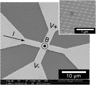
Figure 1: SEM picture of a Hall cross structure with magnetic islands on top, indicating the direction of the current ($I$), magnetic field ($B$) and measured Hall voltage ($V$). The inset shows a zoom of the area with magnetic islands before patterning of the Hall-cross.

II Theory

II.1 Switching field and energy barrier

From statistical measurements of the switching field of a single island it is possible to determine the energy barrier in the absence of an external field ($\Delta U$) and the switching field in the absence of thermal fluctuations ($H_{\text{n}}^{0}$). In the following, we derive the basic theory for linking these values to the measured distribution of the switching field of an individual island.

II.1.1 Thermally induced reversal

Consider a system, like a single domain magnetic island, that has two energy minima, separated by an energy barrier of finite height $\Delta U$. Due to thermal fluctuations, there is a chance that the system jumps between the energy minima. We assume this probability can be described by Arrhenius statistics. At time $\tau$=$0\text{\,}\mathrm{s}$, the system is in one energy minimum. The probability that the system has jumped to the other energy minimum increases with time:

$$P_{\text{sw}}\left(\tau\right) =1-\exp\left(-\tau/\tau_{0}\right),$$ (1)

$$\tau_{0} =\frac{1}{f_{0}}\exp\left(\frac{\Delta U(H,T)}{kT}\right)$$ (2)

where $f_{0}$ is the frequency [Hz] at which the system tries to attempt to overcome the energy barrier, $k$ is Boltzmann’s constant ($1.38\text{\times}{10}^{-23}\text{\,}\mathrm{J}\mathrm{/}\mathrm{K}$) and $T$ the temperature [K].

When taking a hysteresis loop of our magnetic islands, we slowly ramp up the field from some negative field value, where all islands are in the same state, $-H_{\text{sat}}$ in small steps $\Delta H$ and monitor the reversal of the magnetisation in the islands after each step for a waiting time $\Delta\tau$. We assume that the waiting time is short enough to make it very unlikely that there will be multiple reversals, back and forth between the energy minima. In this case, the probability that the magnetisation in the island switches at a field value $H$ is the chance that it switches within the waiting time (Equation 1), multiplied by the chance that it has not yet switched before,

$$\mathcal{P}_{\text{sw}}\left(H,\Delta\tau\right)=\\ P_{\text{sw}}(\Delta\tau)\left(1-\int_{-H_{\text{sat}}}^{H}p_{\text{sw}}\left(H^{\prime},\Delta\tau\right)dH^{\prime}\right).$$ (3)

In the above, $p_{\text{sw}}$ is the corresponding probability density function [m/A]. This implicit equation can be reformulated explicitly if we assume the field steps are so small that we can define a continuous field ramp rate $R=\Delta H/\Delta\tau$ [$\text{\,}\mathrm{A}\text{\,}{\mathrm{m}}^{-1}\text{\,}{\mathrm{s}}^{-1}$]. In that case, the probably density function becomes Engelen et al. (2010)

$$p_{\text{sw}}\left(H,T\right)=\frac{f_{0}}{R}\text{exp}\left(\frac{-\Delta U\left(H,T\right)}{kT}\right)\\ \times\exp\left[-\frac{f_{0}}{R}\int_{-H_{\text{sat}}}^{H}\exp\left(\frac{-\Delta U(H^{\prime},T)}{kT}\right)dH^{\prime}\right].$$ (4)

We explicitly take into account that the energy barrier is dependent on the temperature at which the distribution is measured, because of the variation with temperature of the magnetic properties of the material. However, the crucial information required is the exact way in which the energy barrier, $\Delta U$, decreases with a decrease in strength of the applied field. The relation between the energy barrier and the applied field depends strongly on the way the islands reverse their magnetisation direction. In the following we will describe two extreme models: coherent rotation and domain wall creation and propagation.

II.1.2 Field dependent energy barrier: Coherent rotation

In the coherent rotation model (Stoner–Wohlfarth), we assume that the spins in the island remain parallel during rotation. This model is well described Stoner and Wohlfarth (1991), but repeated here since it defines an upper limit to the switching field that should be compared to alternative models. The model assumes an effective anisotropy $K_{\text{eff}}$ [J], which tries to align the spins parallel to the easy axis at an angle $\theta$, and an external field $H$ that tries to align the spins along the field direction (Figure 2). The total energy of the system is the sum of the anisotropy and the external field energy

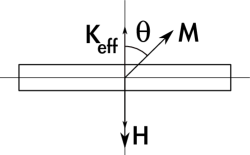
Figure 2: The simplest model discussed assumes that the magnetisation $\boldsymbol{M}$ coherently rotates away from the easy axis $\boldsymbol{K}_{\text{eff}}$ over an angle $\theta$ if the applied field $\boldsymbol{H}$ is increased.

$$U_{\text{I}}=\left(K_{\text{eff}}\sin^{2}\theta+\mu_{0}M_{\text{s}}H\cos\theta\right)V\text{ [J]}$$ (5)

Where $V$ is the sample volume, $M_{\text{s}}$ the sample’s saturation magnetisation [A/m], and $\mu_{0}$ the vacuum permeability [$4\cdot 10^{-7}\pi$ Tm/A]. The extrema in the energy function can be found by equating to zero the derivative of the energy with respect to $\theta$, which leads to $\theta=0$ for the minimum and

$$\cos(\theta_{\text{max}})=\frac{\mu_{0}M_{\text{s}}H}{2K_{\text{eff}}}$$ (6)

for the maximum energy. The energy barrier is the difference between the maximum and minimum,

$$\Delta U_{\text{I}}(H)=K_{\text{eff}}V\left(1-\frac{H}{H^{0}_{\text{I,n}}}\right)^{2}$$ (7)

with the switching field

$$H^{0}_{\text{I,n}}=\frac{2K_{\text{eff}}}{\mu_{0}M_{\text{s}}}\text{ [A/m]}.$$ (8)

We use the upper index $0$ to indicate the switching field in the absence of thermal fluctuation.

Since all spins in the island switch in unison, the switching volume $V_{\text{sw}}$ is equal to the island volume $V$.

II.1.3 Field dependent energy barrier: Domain wall motion

For the $220\text{\,}\mathrm{n}\mathrm{m}$ islands that we measured, the coherent rotation model is too coarse an aproximation. It is more likely that reversal starts in a small region with low anisotropy, followed by the propagation of a domain wall through the island Hu et al. (2005); Lau et al. (2011); Delalande et al. (2012). The theoretical background for this reversal mechanism has been beautifully explained by Adam and co-workers Adam et al. (2012) in their bubble growth model. Their approach, however, lacks the simplicity of the Stoner–Wohlfarth model. We therefore modified their circular geometry to a square shape, while keeping the essence of their model. In contrast to the approach by Adam, this simplified model leads to a closed form solution. Even though our islands are circular, not square, the predicted trends will be very similar. In the following, we describe this diamond model, and discuss its implications for a wall energy density that is either constant or varies with position.

The diamond model

Consider a square magnetic element of thickness $t$ and area $2L^{2}$, with an out of plane easy axis (Figure 3). The magnetisation in the element is pointing downwards, and an opposing field $H$ is applied. Reversal starts by introduction of a domain wall at position $x=0$. The total energy of the system is the sum of the wall energy, proportional to the wall length and the wall energy density $\sigma$ [J/m²], with the external field energy, which is proportional to the area of the reversed domain and the external magnetic field. For $x\leq L$,

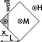
Figure 3: Rather than assuming coherent rotation, it is more realistic to assume creation and propagation of a domain wall. We assume a square island of area $2L^{2}$, into which a domain wall propagates from a corner over a distance $x$.

$$U_{\text{II}} =$$

$$2x\sigma t-2\mu_{0}M_{\text{s}}Ht\left(x^{2}-L^{2}\right) \text{for }x\leq L$$

$$2(2L-x)\sigma t-2\mu_{0}M_{\text{s}}Ht\left(x^{2}-L^{2}\right) \text{for }x>L$$ (9)

The force on the domain wall is the negative derivative of the energy with respect to the wall position $x$. Nucleation of a domain occurs when the force changes sign, which is when the derivative passes zero. The field at which this occurs, $H^{0}_{\text{II,n}}$, is defined as the nucleation field. In the absence of pinning sites, so in a perfectly homogeneous material, the domain wall will continue to propagate until the magnetisation in the island is reversed completely. In this case the nucleation field is equal to the switching field. In reality the domain wall might be trapped Delalande et al. (2012), and next to a nucleation field there will be one or several domain wall depinning fields before the island switches. This case is not considered here.

Constant wall energy

We first consider the wall energy density to be independent of position ($\sigma=\sigma_{0}$). Equating to zero the derivative of the energy with respect to $x$, we obtain, for the wall position at which nuclation occurs,

$$x_{\text{max}}=\frac{\sigma_{0}}{2\mu_{0}M_{\text{s}}H}$$ (10)

We assume $x_{\text{max}}\leq L$, which implies that Equation 10 is only valid for

$$H\geq\frac{\sigma_{0}}{2\mu_{0}M_{\text{s}}L}=H_{\text{L}}$$ (11)

For $H<H_{\text{L}}$, nucleation will occur if the wall reaches the widest part of the diamond, so $x_{\text{max}}=L$.

Figure 4 shows the energy versus the wall position, for both situations. At low fields ($10\text{\,}\mathrm{k}\mathrm{A}\mathrm{/}\mathrm{m}$ in the graph), nucleation occurs when the wall reaches the widest part of the triangle, i.e., at $x_{\text{max}}=L$. At high fields $x_{\text{max}}<L$. As can be seen, the height of the energy barrier, $\Delta U$, depends on the location of the maximum energy, $x_{\text{max}}$. We must consider two cases.

Table 1: Parameters used to generate the graphs of Figures 4 to 9.

$M_{\text{s}}$	$829\text{\,}\mathrm{k}\mathrm{A}\mathrm{/}\mathrm{m}$	$kT$	$25.84\text{\,}\mathrm{m}\mathrm{e}\mathrm{V}$
$\sigma_{0}$	$3.43\text{\,}\mathrm{m}\mathrm{J}\mathrm{/}\mathrm{m}^{2}$	$f_{0}$	${10}^{9}\text{\,}\mathrm{H}\mathrm{z}$
$K_{\text{eff}}$	$386\text{\,}\mathrm{k}\mathrm{J}\mathrm{/}\mathrm{m}^{3}$	$R$	$50\text{\,}\mathrm{A}\mathrm{/}\mathrm{m}\mathrm{s}$
$L$	$50\text{\,}\mathrm{n}\mathrm{m}$	$H_{\text{L}}$	$32.9\text{\,}\mathrm{k}\mathrm{A}\mathrm{/}\mathrm{m}$
$t$	$20\text{\,}\mathrm{n}\mathrm{m}$	$H^{0}_{\text{I,n}}$	$741\text{\,}\mathrm{k}\mathrm{A}\mathrm{/}\mathrm{m}$
$w$	$16\text{\,}\mathrm{n}\mathrm{m}$	$H^{0}_{\text{III,n}}$	$206\text{\,}\mathrm{k}\mathrm{A}\mathrm{/}\mathrm{m}$

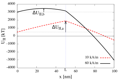
Figure 4: Energy (in units of $kT$ at $300\text{\,}\mathrm{K}$) versus wall position, for a field below $H_{\text{L}}$ where nucleation occurs at $x=L$ (label “a”), and for a field above $H_{\text{L}}$ where nucleation occurs at $x<L$ (label “b”). To generate this plot, we have used the values given in Table 1.

Regime A, $x_{\text{max}}=L$, $H\leq H_{\text{L}}$

At low fields, $H\leq H_{\text{L}}$, the wall must propagate all the way to the widest part of the diamond for nucleation. In this case, $x_{\text{max}}=L$ and the height of the energy barrier is

$$\Delta U_{\text{IIa}}(H) =U_{\text{II}}(L)-U_{\text{II}}(0)$$

$$=2L\sigma_{0}t\left(1-\frac{H}{H^{0}_{\text{II,n}}}\right).$$ (12)

The energy barrier is plotted as a function of the field in Figure 5, we are considering region “IIa” here. The red dashed line shows the extrapolation of the energy barrier for values above $H_{\text{L}}$.

The nucleation field in the absence of thermal activation is equal to

$$H^{0}_{\text{IIa,n}}=\frac{\sigma_{0}}{\mu_{0}M_{\text{s}}L},$$ (13)

which is the intersection of the red dashed line with the $H$-axis. This nucleation field is twice the value of $H_{\text{L}}$, so if there is no thermal activation, this nucleation mechanism will never occur. The maximum field at which reversal in this regime can take place is at $H=H_{\text{L}}$, where the energy barrier $\Delta U_{\text{IIa}}=L\sigma_{0}t$. Using realistic values (Table 1), this energy still is around $800\text{\,}\mathrm{k}\mathrm{T}$, so for our situation nucleation will not occur in regime IIa. The next question is therefore whether nucleation can occur at all before the wall reaches the widest part of the diamond.

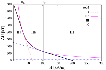
Figure 5: Energy barrier (in units of $kT$ at $300\text{\,}\mathrm{K}$) versus applied field. For fields below $H_{\text{L}}$, nucleation occurs when the wall reaches the widest part of the diamond (regime “IIa”). For larger fields, nucleation is reached before the wall reaches the widest part (regime “IIb”). But in model IIb, the energy barrier never decreases to zero (magenta line). Only if the domain wall energy density is assumed to increase linearly from zero from the edge of the island over a distance $w$, is a reasonable switching field obtained (model III, which is valid for $H>H_{\text{w}}$). The dotted line at $40\text{\,}\mathrm{k}\mathrm{T}$ indicates the energy barrier which can generally not be overcome in normal experimental conditions. To generate this plot, we have taken the values given in Table 1.

Regime B, $x_{\text{max}}<L$, $H>H_{\text{L}}$

At applied fields above $H_{\text{L}}$, nucleation occurs before the wall reaches the widest part of the diamond, $x<L$, and the energy barier equals

$$\Delta U_{\text{IIb}}(H)=U_{\text{II}}(x_{\text{max}})-U_{\text{II}}(0)=\frac{\sigma_{0}^{2}t}{2\mu_{o}M_{\text{s}}H}.$$ (14)

The decrease in the energy barrier with increasing applied field strength is shown in Figure 5, indicated by the solid magenta line “IIb”. The energy barrier never decreases to zero, so $H^{0}_{\text{IIb,n}}=\infty$. By thermal activation however, nucleation can occur at a finite field, in which case the switching volume is

$$V_{\text{sw}}=x_{\text{max}}^{2}t=\frac{\sigma_{0}^{2}t}{4\mu_{0}M_{\text{s}}^{2}H^{2}}.$$ (15)

Figure 6 shows the calculated switching field distribution for model II at room temperature. All switching fields are above $800\text{\,}\mathrm{k}\mathrm{A}\mathrm{/}\mathrm{m}$. The coherent rotation model would give a switching field of $741\text{\,}\mathrm{k}\mathrm{A}\mathrm{/}\mathrm{m}$, which would therefore be the preferred reversal mode, similar to the reversal model discussed in Adam et al. (2012). For our set of parameters, neither regime “IIa” or “IIb” results in realistic switching fields and this model must be discarded.

Figure 6: Thermally activated switching field distribution for a domain wall movement model using a constant wall energy. The switching fields for this oversimplified model are unrealistically high, since they are higher than the nucleation field for coherent rotation in the absence of thermal activation (line at $740\text{\,}\mathrm{k}\mathrm{A}\mathrm{/}\mathrm{m}$).

Linearly increasing wall energy

Since the constant wall energy model above leads to unrealistic values for the nucleation field, we assume a wall energy that increases with position. The simplest assumption is a linear increase, over a distance $w$ (Figure 7).

Figure 7: In the final version of the diamond model, we assume that the domain wall energy increases linearly with distance, as it propagates into the square island, up to $x=w$ (see Figure 3).

When $x<w$, the domain wall is in the linearly increasing part, and the energy as a function of wall position is

$$U_{\text{III}} =2tx^{2}\frac{\sigma_{0}}{w}-2\mu_{0}M_{\text{s}}tH(x^{2}-L^{2})$$

$$=2t\left(\frac{\sigma_{0}}{w}-\mu_{0}M_{\text{s}}H\right)x^{2}+\text{constant}$$ (16)

For $x>w$, the energy is as before in model II. By equating to zero the derivative with respect to $x$, we obtain the nucleation field in the absence of thermal activation:

$$H^{0}_{\text{III,n}}=\frac{\sigma_{0}}{\mu_{0}M_{\text{s}}w}.$$ (17)

The result is similar to model IIa (Equation II.1.3 and 13), with $L$ replaced by $w$. Following the analogue to the line of argument for model IIa, we can discriminate three regions, separated by $H_{\text{L}}$ (Equation (11)) and

$$H_{\text{w}}=\frac{\sigma_{0}}{2\mu_{0}M_{\text{s}}w}=\frac{H^{0}_{\text{III,n}}}{2}.$$ (18)

An example of the energy function is shown in Figure 8. For $H<H_{\text{w}}$, the maximum energy is found at $w<x<L$, and we have the situation of model II. As discussed before, nucleation in this regime does not occur for realistic temperatures. However, for $H_{\text{w}}<H<H^{0}_{\text{III,n}}$, unlike regime IIb, the maximum energy is always found at $x=w$. This is due to the quadratic nature of the energy function for $x<w$. At $H=H^{0}_{\text{III,n}}$, the energy function becomes flat, and the energy barrier disappears.

The energy barrier that is of interest to us is found at $x_{\text{max}}=w$,

$$\Delta U_{\text{III}}(H) =2t\sigma_{0}w\left(1-\frac{H}{H^{0}_{\text{III,n}}}\right)$$ (19)

$$=\Delta U_{0}\left(1-\frac{H}{H^{0}_{\text{III,n}}}\right)$$ (20)

and is displayed together with model II in Figure 5. In contrast to model II, the energy barrier now decreases to zero and nucleation can occur at realistic conditions.

Since the energy barrier is always located at $x_{\text{max}}=w$, the switching volume is simply

$$V_{\text{sw}}=w^{2}t$$ (21)

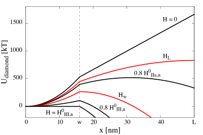
Figure 8: Energy as a function of wall position, assuming a linear increase of wall energy density for $x<w$. For $H<H_{\text{L}}$, the maximum energy is found when the wall reaches the widest part of the diamond ($x=L$). For $H_{\text{L}}<H<H_{\text{w}}$, the maximum energy lies between $x=w$ and $L$. For $H>H_{\text{w}}$, the energy barrier is located at $x=w$, until it disappears at the nucleation field $H^{0}_{\text{III,n}}$.

This diamond model has simple equations for the energy (Equation II.1.3) and energy barrier (Equation 19), nucleation field (Equation 17) and volume (Equation 21). For simplicity we will use in the remainder of this paper

$$H^{0}_{\text{n}}=H^{0}_{\text{III,n}}$$ (22)

The diamond model introduces a new parameter $w$, which is the length over which the domain wall energy increases as the wall enters the island. The rate of increase in domain wall energy $\nicefrac{{\sigma_{0}}}{{w}}$ determines the nucleation field. A reduction in the domain wall energy near the edge of the island is not unrealistic. It could, for instance, be caused by a region of reduced anisotropy at the edge of the island, due to etch damage for instance, or by a finite wall width. If we take a reasonable value for $w$, $16\text{\,}\mathrm{n}\mathrm{m}$, we obtain a quite acceptable value for the nucleation field, as can be seen in Figure 9, which also illustrates how, by moving from the naive model with constant domain wall energy to the edge of the island (red curve II) to a more realistic model with reduced domain wall energy (blue curve III), the nucleation field can be brought below the values for the coherent (Stoner–Wohlfarth) rotation model (black curve I).

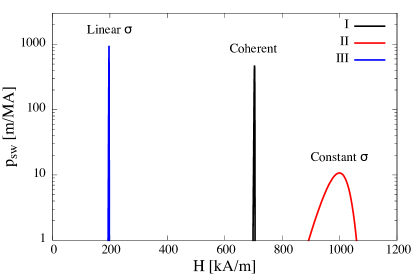
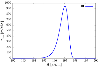
Figure 9: Top: Comparison of the thermally activated switching field distributions of the three different models. The model based on creation and subsequent domain wall movement with a constant wall energy $\sigma$ (red curve II) results in switching fields that are even higher than for a coherent rotation model (black curve I). However, when assuming a domain wall energy density that increases linearly as the wall enters the island, more realistic switching fields are obtained (blue curve III). Bottom: Zoom of the distribution for the final diamond model (III). See Table 1 for parameters used.

Under realistic experimental conditions at room temperature, it is very unlikely that energy barriers of more than $40\text{\,}\mathrm{k}\mathrm{T}$ are overcome by thermal activation. As illustrated by Figure 5, we can safely assume that the energy barrier decreases linearly with the applied field ($n$=1 in our earlier work Engelen et al. (2010)). This is confirmed by Figure 9, which shows that switching below $194\text{\,}\mathrm{k}\mathrm{A}\mathrm{/}\mathrm{m}$ in this example is very unlikely. From Figure 5 we can observe that non-linear effects start at energy barriers above approximately $400\text{\,}\mathrm{k}\mathrm{T}$. One would therefore have to raise the temperature by a factor of ten before any non-linear field dependence could be observed.

It should be noted that from the energy barrier at $H=0$, $\Delta U_{0}$ we can obtain the product $\sigma_{0}w$ (Equation (19)), whereas from the nucleation field in the absence of thermal fluctuation, $H^{0}_{\text{n}}$, we can obtain the ratio $\nicefrac{{\sigma_{0}}}{{w}}$ (Equation (17)). Since both parameters are obtained from the fit of the model to the thermal switching field distribution curves, the domain wall energy and nucleation volume can be determined independently.

$$w=\sqrt{\frac{\Delta U_{0}}{2t\mu_{o}M_{\text{s}}H_{n}^{0}}}$$ (23)

$$\sigma_{0}=\sqrt{\frac{\Delta U_{0}\mu_{o}M_{\text{s}}H_{n}^{0}}{2t}}$$ (24)

The nucleation volume can therefore also be written as

$$V_{\text{sw}}=w^{2}t=\frac{\Delta U_{0}}{2\mu_{0}M_{\text{s}}H^{0}_{n}}.$$ (25)

II.2 Temperature dependence of the magnetisation and anisotropy

Material parameters such as saturation magnetisation and magnetic anisotropy constant are temperature dependent. To obtain an estimate for the magnitude of this effect when we cool down to low temperatures in our experiments, we assume a simple Brillouin theory (taken from Coey (2010) with $J=2$) for the temperature dependence of the saturation magnetisation.

$$M_{\text{s}}(T)/M_{\text{s}}(0)=\left(\frac{5}{4}\text{coth}\frac{5}{4}\chi-\frac{1}{4}\text{coth}\frac{\chi}{4}\right)$$ (26)

where the value of $\chi$ can related to the Curie temperature $T_{\text{c}}$ using

$$M_{\text{s}}(T)/M_{\text{s}}(0)=\left(\frac{T}{2T_{\text{c}}}\right)\chi$$ (27)

The value of $\chi$ can be obtained graphically or by symbolic mathematical manipulation software. We use this model to extrapolate the measured values of $M_{\text{s}}(T)$ to $M_{\text{s}}(0)$.

We assume that the total magnetic anisotropy $K_{\text{eff}}$ has two contributions: the demagnetisation energy $K_{\text{d}}(T)$, which is equal to $\nicefrac{{1}}{{2}}\mu_{0}M_{\text{s}}^{2}$, and an intrinsic anisotropy $K_{\text{u}}(T)$. Depending on the mechanism causing the intrinsic anisotropy, the magnetisation dependence can be on the order of $M_{\text{s}}^{2}$ (e.g. for crystalline anisotropy Staunton et al. (2006)) all the way up to order $M_{\text{s}}^{3}$ for pure surface anisotropy Asselin et al. (2010). Therefore we model the temperature dependence of the effective anisotropy as

$$K_{\text{eff}}(T)=K_{\text{u}}(0)\alpha^{n}-K_{\text{d}}(0)\alpha^{2}$$ (28)

With $n=2$ or $3$ and

$$\alpha=\left(\frac{5}{4}\text{coth}\frac{5}{4}\chi-\frac{1}{4}\text{coth}\frac{\chi}{4}\right)$$ (29)

III Experimental

III.1 Preparation of the thin magnetic film

The magnetic multilayer samples are prepared by cleaning $\left<100\right>$ p-type wafers and stripping them the native oxide. A thermal oxide layer of $50\text{\,}\mathrm{nm}$ is grown by an LPCVD process. The SiO₂ acts as an insulating layer between the conducting metal layer and the bulk silicon. A multi-target DC sputtering system is used to deposit all metal layers in one single run without breaking the vacuum. The thickness of each layer is controlled by opening and closing the shutters in front of the sputter guns. The base pressure of the system was lower than $0.5\text{\,}\mathrm{\SIUnitSymbolMicro Pa}$ with deposition pressures of $1\text{\,}\mathrm{Pa}$ for the Ta layers and $0.8\text{\,}\mathrm{Pa}$ for the Co and Pt using Ar gas.

The seedlayers for the multilayer samples consist of $5\text{\,}\mathrm{nm}$ Ta and $25\text{\,}\mathrm{nm}$ Pt. A bilayer of $0.3\text{\,}\mathrm{nm}$ Co and $0.3\text{\,}\mathrm{nm}$ Pt is deposited with 34 repetitions resulting in a $20(1)\text{\,}\mathrm{nm}$ magnetic layer. The capping for the samples consists of $3\text{\,}\mathrm{nm}$ Pt, which prevents oxidation of the Co.

III.2 Patterning of arrays of islands

Laser interference lithography (LIL) is used to create a pattern in a photoresist layer, which acts as an etching mask.

The pattern is first transferred into the bottom anti-reflective coating (BARC) by O₂ reactive ion beam etching (RIBE). The BARC layer (DUV-30 J8) improves the resist pattern by limiting standing waves caused by interference of the incoming waves with reflections from the metal layers. The pattern is then transferred into the magnetic layer by Ar ion beam etching (IBE). All etching steps were performed in an Oxford i300 reactive ion beam etcher.

After etching, the resulting samples have a Ta/Pt seedlayer with magnetic islands on top. The average diameter of the islands is approximately $220\text{\,}\mathrm{nm}$ with a centre-to-centre pitch of $600\text{\,}\mathrm{nm}$.

A lithography process is used to define Hall cross structures in a layer of photoresist, similar as in our previous workEngelen et al. (2010). The Hall cross structures are transferred into the insulating layer using Ar IBE to ensure that during the Hall measurement, the current only runs through a small ensemble of islands.

The resulting structure consists of a conducting Hall cross of Ta/Pt with magnetic islands with a diameter of $220\text{\,}\mathrm{nm}$ and a pitch of $600\text{\,}\mathrm{nm}$ on top as shown in the SEM micrograph in Figure 1.

III.3 Temperature dependent AHE

The anomalous Hall measurements are performed in an Oxford superconducting magnet. Using a temperature controller and a cryostat, the measurements are taken between $5\text{\,}\mathrm{K}$ and $300\text{\,}\mathrm{K}$. The magnetic field is applied perpendicularly to the sample plane. An AC current at a frequency of $12\,333\text{\,}\mathrm{Hz}$ is applied to the Hall cross, and the Hall signal is measured using a lock-in amplifier.

For the statistical measurements of Figure 11, the switching field is measured over 150 times. During the acquisition, the temperature variation from the setpoint is less than $0.1\text{\,}\mathrm{K}$. The measurements are performed with a field sweep rate $R$ of $39\text{\,}\mathrm{A}\text{\,}{\mathrm{m}}^{-1}\text{\,}{\mathrm{s}}^{-1}$ at $300\text{\,}\mathrm{K}$ and $3.9\text{\,}\mathrm{A}\text{\,}{\mathrm{m}}^{-1}\text{\,}{\mathrm{s}}^{-1}$ at $10\text{\,}\mathrm{K}$.

Since the variation of the switching field with temperature differs between islands, the order of switching can change with the temperature. This is especially true for weak islands. We took great care to avoid mix-ups by comparing the step heights in the hysteresis loops, so that the island we measure at $10\text{\,}\mathrm{K}$ is the same island as the one we measure at $300\text{\,}\mathrm{K}$. Since the mechanism which causes the weak and strong island to differ is expected to be the same for each island, an accidental mix up between two islands with similar switching field will have limited effect on the final results. The switching fields of a strong island are separated further apart, and a change in reversal order is unlikely.

For the temperature dependent measurement, shown in Figure 12, the field is swept between sample saturation levels at a constant rate $R$ of $39\text{\,}\mathrm{A}\text{\,}{\mathrm{m}}^{-1}\text{\,}{\mathrm{s}}^{-1}$. The temperature is kept constant during the measurement and deviations from the setpoint are less than $0.5\text{\,}\mathrm{K}$ at the switching event.

III.4 Magnetic characterisation

The temperature dependence of the saturation magnetisation of the continous, unpatterned film ($M_{\text{s}}(T)$) is determined using a VSM. The sample temperature is regulated using a flow of nitrogen cooling gas and a heater element.

The effective anisotropy at room temperature is determined by a home built torque magnetometer. A DMS VSM-10 is used to determine the temperature dependence of the effective anisotropy from the saturation field, using the torque measurement at room temperature as scaling factor.

IV Results

IV.1 Temperature dependent reversal

Figure 10 shows the upgoing part of the hysteresis loop taken by AHE on the array of approximately $80$ islands at room temperature as well as $10\text{\,}\mathrm{K}$). When the temperature is decreased, the switching field increases. The AHE measurements are compared to VSM measurements at room temperature of an $8$$\times$$8\text{\,}\mathrm{m}\mathrm{m}$ sample with almost $200$ million islands. To enable comparison, the loops were scaled to the saturation moment. The switching field distribution in the VSM loop is higher, which can be attributed to the larger measurement area.

The AHE hysteresis loop shows small steps, which are caused by the reversal of individual islands. The the field ramp rate is adapted in such a way that we capture a switching event of a weak island, switching at low field, and a strong island with a high switching field. To save time, the intermediate field range is traversed more quickly. Figure 10 shows four zooms, for a weak and a strong island at 10 and $300\text{\,}\mathrm{K}$.

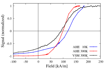
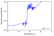
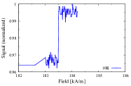
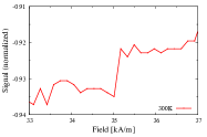
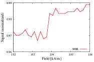
Figure 10: Top: Upward branch of AHE hysteresis curves at room temperature and $10\text{\,}\mathrm{K}$ of an array of $80$ islands, compared to a VSM hysteresis curve of a $8$$\times$$8\text{\,}\mathrm{m}\mathrm{m}$ sample with almost $200$ million islands at room temperature. Bottom: In the AHE measurements, switching of individual islands can be observed. We compared weak islands, that switch at low fields, to strong islands switching at high fields.

IV.2 Temperature dependence of the thermal switching field distribution

Figure 11 shows the thermally activated switching field distribution at $10\text{\,}\mathrm{K}$ and $300\text{\,}\mathrm{K}$ for one of the first islands that switches (weak) and one of the last islands (strong) when ramping the field from -$H_{\text{sat}}$ to $H_{\text{sat}}$. During cooling, two effects occur. In the first place, the average switching field increases. Secondly, the width of the distribution decreases dramatically. We can quantify this by dividing the full width at half maximum of the distributions ($\Delta H$) by the field at which the maximum in the distribution occurs ($H_{\text{M}}$). These values are tabulated in Table 2 for the measurements on both the strong and weak island. The relative distribution width $\Delta H/H_{\text{M}}$ drops by one order of magnitude when the temperature is decreased to $10\text{\,}\mathrm{K}$, which illustrates that the origin of the variation in switching fields is indeed thermal fluctuation. The same observation has been made for $75\text{\,}\mathrm{n}\mathrm{m}$ diameter Co/Ni multilayered islands Gopman et al. (2013).

Table 2: Values for the full width at half maximum ($\Delta H$) divided by the field with the highest occurence ($H_{\text{M}})$) as a measure for the thermal switching field distribution.

		$10\text{\,}\mathrm{K}$	$300\text{\,}\mathrm{K}$
Weak	$\Delta H$ [$\mathrm{k}\mathrm{A}\mathrm{/}\mathrm{m}$]	0.29	1.97
	$H_{\text{M}}$ [$\mathrm{k}\mathrm{A}\mathrm{/}\mathrm{m}$]	84.7	34.7
	$\Delta H$/$H_{M}$	0.0034	0.057
Strong	$\Delta H$ [$\mathrm{k}\mathrm{A}\mathrm{/}\mathrm{m}$]	0.23	1.60
	$H_{\text{M}}$ [$\mathrm{k}\mathrm{A}\mathrm{/}\mathrm{m}$]	184	153
	$\Delta H$/$H_{M}$	0.0012	0.010

The distributions are fitted to Equation 4, with $\Delta U_{0}$ and $H_{\text{n}}^{0}$ as fitting parameters. The results of the fit are given in Table 3 under the caption “Statistical fit”. When decreasing the temperature from 300 to $10\text{\,}\mathrm{K}$, the switching field in the absence of thermal activation $H_{\text{n}}^{0}$ increases. The increase is more substantial for the weak island (40%) than for the strong island (9%). The observed increase in the average switching field in Figure 11 is therefore not only caused by a reduction of thermal energy, other effects must also be taking place.

For both weak and strong islands, the energy barrier $\Delta U_{0}$ decreases upon cooling (by a factor of 2.7 and 3.7 respectively). From the values of $\Delta U_{0}$ and $H_{\text{n}}^{0}$, we can calculate the domain wall energy $\sigma_{0}$ and the width of the region of reduced domain wall energy $w$, using the diamond model for reversal (Equations 23 and 24). The substantial decrease in the energy barrier seems to be caused by a strong decrease in $w$ (a factor of two), with its ensuing decrease in the switching volume ($w^{2}t$), and, but much less so, by a decrease in the domain wall energy (20% to 50% respectively).

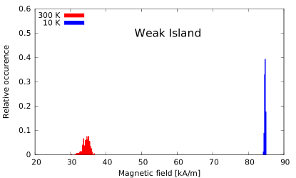
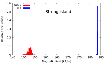
Figure 11: Histograms of the switching field of over 150 reversal incidents of a weak and strong island measured at 10.0(1) K and 300.0(1) K. The bins are normalised to the total amount of reversals, so that the integral under the curves equals one. The width of each bin in the histogram is $0.16\text{\,}\mathrm{kA}\text{\,}{\mathrm{m}}^{-1}$.

Table 3: Switching field H${}_{\text{n}}^{0}$ and energy barrier $\Delta U_{0}$ in the absence of thermal fluctuations determined from the fits to the thermal dependence of the switching field (in Figure 12) and from fitting the statistical measurements of the reversal of a weak and a strong island at $10\text{\,}\mathrm{K}$ and $300\text{\,}\mathrm{K}$ (Figure 11). From these values we can estimate the domain wall energy $\sigma_{0}$ and the width of the reduced domain wall energy region $w$ (Figure 7). The values in parentheses show the $95\text{\,}\mathrm{\char 37\relax}$ confidence intervals obtained from the fit (H${}_{\text{n}}^{0}$ and $\Delta U_{0}$) and combined measurement parameter errors ($w$ and $\sigma_{0}$).

	Temperature fit		Statistical fit
Weak	I	II	10 K	300 K
H${}_{\text{n}}^{0}$ [$\mathrm{k}\mathrm{A}\mathrm{/}\mathrm{m}$]	75.08(2)	93.14(1)	87.28(3)	53.6(1)
$\Delta U_{0}$ [$\mathrm{eV}$]	1.28(1)	2.0(7)	0.65(1)	1.74(1))
$w$ [$\mathrm{n}\mathrm{m}$]	7.9(3)	9(2)	5.2(3)	11.0(5)
$\sigma_{0}$ [$\mathrm{m}\mathrm{J}\mathrm{/}\mathrm{m}^{2}$]	0.65(1)	0.9(2)	0.50(2)	0.64(4)
Strong		I	10 K	300 K
H${}_{\text{n}}^{0}$ [$\mathrm{k}\mathrm{A}\mathrm{/}\mathrm{m}$]		183(2)	185.52(2)	168.24(8)
$\Delta U_{0}$ [$\mathrm{eV}$]		2.7(4)	1.78(1)	6.74(3))
$w$ [$\mathrm{n}\mathrm{m}$]		7.4(9)	6.0(3)	12.2(5)
$\sigma_{0}$ [$\mathrm{m}\mathrm{J}\mathrm{/}\mathrm{m}^{2}$]		1.5(2)	1.20(5)	2.22(9)

IV.3 Temperature dependence of average switching field

In addition to distributions at 10 and $300\text{\,}\mathrm{K}$, we used the anomalous Hall effect to estimate the average switching field from single hystersis loops. Figure 12 shows the temperature dependence of the average switching field of one strong and two weak islands. The measurements are fitted to the theory from Equation 4, using the energy barriers for the diamond model (Equation 19) and under the restriction that the fitting parameters do not change with temperature. The figure shows that the actual temperature dependence of the strong island is slightly lower than predicted by the model, whereas that of the weak islands is slightly higher. This is an indication that assuming the temperature independence of the material parameters is incorrect.

The fitting parameters $H_{n}^{0}$ and $\Delta U_{0}$ are tabulated in Table 3 under the caption “Temperature Fit”. The values of $H_{\text{n}}^{0}$ agree well with those obtained from the distributions at $10\text{\,}\mathrm{K}$, but are higher than those obtained at $300\text{\,}\mathrm{K}$. The energy barrier estimated from the temperature dependence of the average switching field is, however, much larger than that obtained from the distribution at $10\text{\,}\mathrm{K}$. This again clearly demonstrates that assuming temperature independent material parameters leads to incorrect conclusions about the thermal stability of the islands. The value of the energy barrier of the strongest island is in agreement with that estimated by Kikuchi et al Kikuchi et al. (2011) ($5.5\text{\,}\mathrm{e}\mathrm{V}$) on a $300\text{\,}\mathrm{n}\mathrm{m}$ diameter island prepared from a [Co($0.9\text{\,}\mathrm{n}\mathrm{m}$)/Pt($2\text{\,}\mathrm{n}\mathrm{m}$)]₃ multilayer. The estimate for the nucleation field in the absence of thermal fluctuations is $0.4\text{\,}\mathrm{M}\mathrm{A}\mathrm{/}\mathrm{m}$, which is higher by a factor of two than that in our experiment. The difference could be caused by the better defined interfaces, due to the thicker Co layer, and the reduced number of bilayers. One should however also take into consideration that in their work, a coherent rotation model was assumed, which leads to higher values for the estimate of the energy barrier and the switching field Engelen et al. (2010).

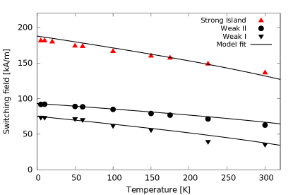
Figure 12: Temperature dependent average switching field for a weak and a strong island using temperature dependent AHE measurements. The lines are fitted using Equation 4 with the energy barriers given by Equation 19 , under the condition that the switching volume $V_{\text{sw}}$ (Equation 25) is independent of temperature.

IV.4 Temperature dependence of the material parameters

To gain insight into the temperature dependence of the material parameters, we measured VSM hysteresis loops from $170\text{\,}\mathrm{K}$ up to room temperature. From these loops the saturation magnetisation and anisotropy are estimated.

IV.4.1 Temperature dependence of the saturation magnetisation

Figure 13 shows that indeed the saturation magnetisation decreases slightly with increasing temperature. The curve is fitted to the Brillouin function (Equations 26 and 27), with fitting parameters the Curie temperature ($T_{\text{c}}$) and the saturation magnetisation at 0 K ($M_{\text{s}}(0)$). The Curie temperature is estimated to be $684(58)\text{\,}\mathrm{K}$, which is in agreement with previous studies of Co/Pt multilayers Meng (1996); van Kesteren and Zeper (1993). The value of $M_{\text{s}}(0)$ is estimated to be $888(9)\text{\,}\mathrm{k}\mathrm{A}\mathrm{/}\mathrm{m}$. To estimate the errors of the fit, a Monte Carlo method is used, where we assumed $\sigma_{T}$=$7\text{\,}\mathrm{K}$ and $\sigma_{M_{\text{s}}(T)}$=$10\text{\,}\mathrm{kA}\text{\,}{\mathrm{m}}^{-1}$.

From the fit we can conclude that the saturation magnetisation decreases by about 7% when increasing the temperature from 10 to $300\text{\,}\mathrm{K}$. By itself, this is not sufficient to explain the large variation in $H_{\text{n}}^{0}$. Shan et al. Shan et al. (1994) report a much stronger decrease in magnetisation, by 22%, for a similar Co layer thickness, but much thicker Pt thickness ($1.5\text{\,}\mathrm{n}\mathrm{m}$). The dependence they measured however does not resemble a Brillouin function.

It any case, it is clear that the magnetisation changes, and we may expect that other material parameters change as well. Therefore, we also estimated the anisotropy from the VSM hysteresis loops.

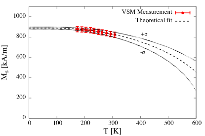
Figure 13: Temperature dependence of $M_{\text{s}}$ from temperature dependent VSM measurements on the continuous film and a fit using Equations 26 and 27. The $\sigma$ lines indicate the 68.2% confidence intervals.

IV.4.2 Temperature dependence of the anisotropy

Figure 14 shows the anisotropy of the continuous film as a function of the temperature, obtained by VSM, using a room temperature torque measurement for calibration. Equation 28 is fitted to the measured $K_{\text{eff}}(T)$ with the fitted parameters $T_{\text{c}}$, $M_{\text{s}}(0)$ and $K_{\text{u}}(0)$, where the value of the exponent $n$ is either of the two extremes. Given the uncertainty in the estimate of the anisotropy, and the limited temperature range, it is impossible to determine which exponent is correct. Table 4 shows the fitted parameters for both cases. To obtain an estimate of the measurement errors in the fitted parameters, again a Monte Carlo method is used, for which we assumed the uncertainty in the temperature to have a standard deviation of $3.5\text{\,}\mathrm{K}$, and $6\text{\,}\mathrm{k}\mathrm{J}\mathrm{/}\mathrm{m}^{3}$ in the values of $K_{\text{eff}}$.

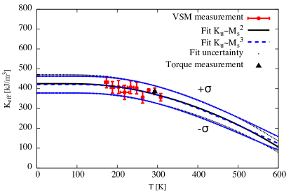
Figure 14: Temperature dependent anisotropy VSM measurements and torque measurement at room temperature on the continuous film. The theoretical fits are created using Equation 28 for exponent $n$=2 or 3. The $\sigma$ lines indicate the 68.2% confidence intervals of the fits.

Table 4: Fitted parameters for the temperature dependence of the effective anisotropy (Figure 14), assuming the effective anisotropy is proportional to $M_{\text{s}}^{2}$ or $M_{\text{s}}^{3}$.

	$n$=2	$n$=3
$K_{\text{u}}$ [$\mathrm{M}\mathrm{J}\mathrm{/}\mathrm{m}^{3}$]	$0.91(2)\text{\,}$	$0.89(2)\text{\,}$
$M_{\text{s}}$ [$\mathrm{M}\mathrm{A}\mathrm{/}\mathrm{m}$]	$0.89(2)\text{\,}$	$0.86(2)\text{\,}$
$T_{\text{c}}$ [$\mathrm{K}$]	$679(15)\text{\,}$	$872(20)\text{\,}$

The exact value of the exponent in Equation 28 has very little effect on the estimate of the anisotropy and magnetisation of the film. Assuming the exponent to lie somewhere between the two extrema, the fitted value of $M_{\text{s}}(0)$=$0.87(4)\text{\,}\mathrm{M}\mathrm{A}\mathrm{/}\mathrm{m}$ is equal, within the estimation error, to the value found from extrapolation of the $M_{\text{s}}(T)$ curve ($0.888(9)\text{\,}\mathrm{M}\mathrm{A}\mathrm{/}\mathrm{m}$, see Figure 13). The similarly estimated value of $K_{\text{u}}(0)$ is $0.90(3)\text{\,}\mathrm{M}\mathrm{J}\mathrm{m}^{-3}$.

The value of the exponent does however have a significant effect on the estimate for the Curie temperature $T_{\text{c}}$. The estimated Curie temperature for $n$=2 is, within the measurement error, equal to the estimate we obtained from the temperature dependence of the magnetisation ($684(58)\text{\,}\mathrm{K}$), which is in agreement with previous studies. This suggests that the intrinsic anisotropy in the film ($K_{\text{u}}$) is rather more proportional to $M_{\text{s}}^{2}$ than to $M_{\text{s}}^{3}$. This seems to indicate that the origin of the perpendicular anisotropy is not only due to interface anisotropy. A wider temperature range might help to narrow down the estimates, but it should be noted that at temperatures above $500\text{\,}\mathrm{K}$, the Co/Pt interfaces start to mix.

V Discussion

When we apply the diamond model to the measured thermally activated switching field distributions, we conclude that difference between islands is primarily caused by a difference in wall energy $\sigma_{0}$, and much less due to a difference in transition region $w$. Why the domain wall energy varies between islands cannot be determined from Anomalous Hall measurements only. A possible cause for a reduction in wall energy might be edge damage caused by the ion beam etching process, leading to mixing between the Co and Pt layers and loss of interface anisotropy. Also edge roughness caused by the lithography might play a role, since it will strongly influence the way the domain wall enters the island.

Based on previous reports and our observations, we can conclude that both the magnetisation and anisotropy decrease with increasing temperature. It is very unlikely that the exchange constant $A$ increases, since it generally decreases with magnetisation Goll et al. (2004). Since the wall energy is proportional to $\sqrt{AK_{\text{u}}}$, it should decrease as the temperature increases. This is in contradiction with the fit to the distributions, from which we conclude that the wall energy increases by 20% to 50%. The origin of this apparent discrepancy should be the subject of further study.

In addition to a moderate increase in the domain wall energy, our simple diamond model predicts a strong increase of the switching volume with increasing temperature. If the region of reduced wall energy $w$ is somehow related to the wall thickness (proportional to $\sqrt{\nicefrac{{A}}{{K_{\text{u}}}}}$), we would also expect a large variation in the wall energy (proportional to $\sqrt{AK_{\text{u}}}$). However, this is not the case. If $w$ is due to etch damage during the fabrication process or edge roughness, there is a possibility that the temperature dependency remains, or even increases. This point also deserves further investigation.

The interpretation of the thermally activated distributions depends on having good models for the thermal stability (Equation (4)) and the relation between the energy barrier and the strength of the applied field (Equation (19)). Since the model for thermal stability is well established, and fits almost perfectly to the distributions, we assume that it is correct. Our diamond model is simple, but a more elaborate micromagnetic model, along the lines of Adam Adam et al. (2012), will not resolve the above contradictions since it is based on the same assumptions and differs only in a more realistic island shape and anisotropy distribution. For furher refinement, one might have to include the possibility that reversal can take place over multiple pathways Roy and Kumar (2017), each of which can have a different temperature dependence.

It is without doubt, however, that the temperature dependence of the material parameters is substantial. Determining the energy barrier from the distribution of the switching fields of the individual islands at the temperature of interest is therefore to be preferred.

VI Conclusion

By means of the very sensitive anomalous Hall effect, we have been able to measure the reversal of individual magnetic islands of diameter $220\text{\,}\mathrm{n}\mathrm{m}$ in an array of approximately eighty islands with a centre-to-centre pitch of $600\text{\,}\mathrm{n}\mathrm{m}$. By traversing the hysteresis loop more than 150 times, we have observed that the switching field of an individual island fluctuates by about $10\text{\,}\mathrm{k}\mathrm{A}\mathrm{/}\mathrm{m}$. When reducing the temperature, this variation for a single island decreases significantly, which proves that the cause of the fluctuations is thermal energy in the system.

From the distribution in switching fields of a single island, we can estimate the switching field in the absence of thermal fluctuations, $H_{n}^{0}$, and the energy barrier at zero field, $\Delta U_{0}$. This estimate requires a model that relates the decrease in the energy barrier with an increase in the externally applied field. We developed a simple “diamond” model, based on creation and the subsequent propagation of a domain wall. Reasonable nucleation fields can only be achieved if we assume the domain wall energy to increase from zero as the wall enters the island, up to a maximum value after a certain distance $w$ from the edge of the island.

From the model fit to the thermal switching field distributions, we estimate that $H_{n}^{0}$ decreases when the temperature increases from 10 to $300\text{\,}\mathrm{K}$. The temperature dependence is more prominent for weak islands (approximately 40%), than for strong islands (approximately 10%). The energy barrier on the other hand has a much stronger dependence (it increases by a factor of three to four). Translated to the parameters of the diamond model, the increase in the energy barrier is mainly due to an increase in the switching volume ($w^{2}t$), which increases by a factor of two, and much less due to an increase in the domain wall energy ($\sigma_{0}$), which increases by 20% to 50%.

The switching field in the absence of thermal energy, $H_{n}^{0}$, does not necessarily have to be identical to the switching field measured at $0\text{\,}\mathrm{K}$, since the material parameters will vary with temperature. When we extrapolate the switching field to $0\text{\,}\mathrm{K}$, we find values that are almost identical to $H_{n}^{0}$ measured at $10\text{\,}\mathrm{K}$, which is substantially higher than the $H_{n}^{0}$ measured at $300\text{\,}\mathrm{K}$. The energy barrier determined from the dependence of the switching field on temperature is also strongly overestimated, by at least a factor of two for the weakest island and 30% for the strongest compared to the measurement at $10\text{\,}\mathrm{K}$.

That the material parameters do vary with temperature is illustrated by temperature dependent VSM measurements, which show that the magnetisation decreases by $7\text{\,}\mathrm{\char 37\relax}$ and anisotropy by $16\text{\,}\mathrm{\char 37\relax}$ when increasing the temperature from 10 to $300\text{\,}\mathrm{K}$.

However, whichever method is used, the value of $w$ is similar for weak and strong islands and varies from 5 to $12\text{\,}\mathrm{n}\mathrm{m}$. The domain wall energy for weak islands (0.5 to $1\text{\,}\mathrm{m}\mathrm{J}\mathrm{/}\mathrm{m}^{2}$) is clearly lower than that for strong islands (1.2 to $2.3\text{\,}\mathrm{m}\mathrm{J}\mathrm{/}\mathrm{m}^{2}$). Within the framework of our model, we must therefore conclude that the variation in the switching fields between islands must be caused by variations in domain wall energy.

Our work demonstrates that detailed observations of the fluctuations in the switching fields of individual islands allows us to determine the basic parameters of the energy barrier between magnetisation states, such as the height of the energy barrier (important for thermal stability) and the field required to overcome this barrier in the absence of thermal fluctuations (important for ultra-fast switching). In contrast to temperature dependent measurements, which rely on the assumption that the material parameters are temperature independent, our method allows us to determine these parameters at any temperature. This is important, for instance, for applications working at room temperature, such as data storage in bit patterned media, magnetic random access memories, and magnetic logic circuits.

References

- Schuh et al. (2001) D. Schuh, J. Biberger, A. Bauer, W. Breuer, and D. Weiss, IEEE Trans. Magn. 37, 2091 (2001), doi:10.1109/20.951063.
- Wernsdorfer et al. (1997) W. Wernsdorfer, E. Bonet Orozco, K. Hasselbach, A. Benoit, B. Barbara, N. Demoncy, A. Loiseau, H. Pascard, and D. Mailly, Phys. Rev. Lett. 78, 1791 (1997), doi:10.1103/PhysRevLett.78.1791.
- Wierenga et al. (2000) H. A. Wierenga, E. Janssen, S. E. Stupp, and J. P. C. Bernards, J. Magn. Magn. Mater. 210, 35 (2000), doi:10.1016/S0304-8853(99)00626-5.
- Sharrock (1994) M. P. Sharrock, J. Appl. Phys. 76, 6413 (1994), doi:10.1063/1.358282.
- Victora (1989) R. H. Victora, Phys. Rev. Lett. 63, 457 (1989), doi:10.1103/PhysRevLett.63.457.
- Sharrock and McKinney (1981) M. P. Sharrock and J. T. McKinney, IEEE Trans. Magn. 17, 3020 (1981), doi:10.1109/TMAG.1981.1061755.
- Collocott and Neu (2012) S. Collocott and V. Neu, Journal of Physics D: Applied Physics 45 (2012), doi:10.1088/0022-3727/45/3/035002.
- Ito et al. (2008) A. Ito, N. Kikuchi, S. Okamoto, and O. Kitakami, IEEE Transactions on Magnetics 44, 3446 (2008), doi:10.1109/TMAG.2008.2002630.
- Engelen et al. (2010) J. B. C. Engelen, M. Delalande, A. J. le Fèbre, T. Bolhuis, T. Shimatsu, N. Kikuchi, L. Abelmann, and J. C. Lodder, Nanotechnol. 21, 035703 (2010), doi:10.1088/0957-4484/21/3/035703.
- de Vries et al. (2013) J. de Vries, T. Bolhuis, and L. Abelmann, J. Appl. Phys. 113, 17B910 (2013), doi:10.1063/1.4801399.
- Yun et al. (2014) S.-J. Yun, S.-C. Yoo, S.-B. Choe, and B.-C. Min, Journal of the Korean Physical Society 65, 1607 (2014), doi:10.3938/jkps.65.1607.
- Chen et al. (2010) Y. Chen, J. Ding, J. Deng, T. Huang, S. Leong, J. Shi, B. Zong, H. Ko, C. Au, S. Hu, et al., IEEE Transactions on Magnetics 46, 1990 (2010), doi:10.1109/TMAG.2010.2043064.
- Thomson et al. (2006) T. Thomson, G. Hu, and B. D. Terris, Phys. Rev. Lett. 96, 257204 (2006), doi:10.1103/PhysRevLett.96.257204.
- Shaw et al. (2007) J. M. Shaw, W. H. Rippard, S. E. Russek, T. Reith, and C. M. Falco, J. Appl. Phys. 101, 023909 (2007), doi:10.1063/1.2431399.
- Breitkreutz et al. (2015) S. Breitkreutz, A. Fischer, S. Kaffah, S. Weigl, I. Eichwald, G. Ziemys, D. Schmitt-Landsiedel, and M. Becherer, Journal of Applied Physics 117 (2015), doi:10.1063/1.4906440.
- Wang et al. (2004) H.-T. Wang, S. T. Chui, A. Oriade, and J. Shi, Phys. Rev. B 69, 064417 (2004), doi:10.1103/PhysRevB.69.064417.
- Wang et al. (2008) X. Wang, Y. Zheng, H. Xi, and D. Dimitrov, Journal of Applied Physics 103 (2008), doi:10.1063/1.2837800.
- Banholzer et al. (2011) A. Banholzer, R. Narkowicz, C. Hassel, R. Meckenstock, S. Stienen, O. Posth, D. Suter, M. Farle, and J. Lindner, Nanotechnology 22 (2011), doi:10.1088/0957-4484/22/29/295713.
- Stoner and Wohlfarth (1991) E. Stoner and E. Wohlfarth, IEEE Transactions on Magnetics 27, 3475 (1991), doi:10.1109/TMAG.1991.1183750.
- Hu et al. (2005) G. Hu, T. Thomson, C. T. Rettner, and B. D. Terris, IEEE Trans. Magn. 41, 3589 (2005), doi:10.1109/TMAG.2005.854733.
- Lau et al. (2011) J. Lau, X. Liu, R. Boling, and J. Shaw, Physical Review B - Condensed Matter and Materials Physics 84 (2011), doi:10.1103/PhysRevB.84.214427.
- Delalande et al. (2012) M. Delalande, J. de Vries, L. Abelmann, and J. C. Lodder, J. Magn. Magn. Mater. 324, 1277 (2012), doi:10.1016/j.jmmm.2011.09.037.
- Adam et al. (2012) J.-P. Adam, S. Rohart, J.-P. Jamet, J. Ferré, A. Mougin, R. Weil, H. Bernas, and G. Faini, Phys. Rev. B 85, 214417 (2012), doi:10.1103/PhysRevB.85.214417.
- Coey (2010) J. M. D. Coey, Magnetism and magnetic materials (Cambridge University Press, 2010).
- Staunton et al. (2006) J. Staunton, L. Szunyogh, A. Buruzs, B. Gyorffy, S. Ostanin, and L. Udvardi, Physical Review B - Condensed Matter and Materials Physics 74 (2006), doi:10.1103/PhysRevB.74.144411.
- Asselin et al. (2010) P. Asselin, R. F. L. Evans, J. Barker, R. W. Chantrell, R. Yanes, O. Chubykalo-Fesenko, D. Hinzke, and U. Nowak, Phys. Rev. B 82, 054415 (2010), doi:10.1103/PhysRevB.82.054415.
- Gopman et al. (2013) D. Gopman, D. Bedau, G. Wolf, S. Mangin, E. Fullerton, J. Katine, and A. Kent, Physical Review B - Condensed Matter and Materials Physics 88 (2013), doi:10.1103/PhysRevB.88.100401.
- Kikuchi et al. (2011) N. Kikuchi, Y. Suyama, S. Okamoto, and O. Kitakami, Journal of Applied Physics 109 (2011), doi:10.1063/1.3540405.
- Meng (1996) Q. Meng, Ph.D. thesis, University of Twente (1996).
- van Kesteren and Zeper (1993) H. W. van Kesteren and W. B. Zeper, J. Magn. Magn. Mater. 120, 271 (1993), doi:10.1016/0304-8853(93)91339-9.
- Shan et al. (1994) Z. S. Shan, J. X. Shen, R. D. Kirby, D. J. Sellmyer, and Y. J. Wang, J. Appl. Phys. 75, 6418 (1994), doi:10.1063/1.355370.
- Goll et al. (2004) D. Goll, H. Kronmüller, and H. Stadelmaier, Journal of Applied Physics 96, 6534 (2004), doi:10.1063/1.1809250.
- Roy and Kumar (2017) A. Roy and P. Kumar, Journal of Magnetism and Magnetic Materials 424, 69 (2017), doi:10.1016/j.jmmm.2016.09.070.