Imprint of non-linear effects on HI intensity mapping on large scales

Abstract

Intensity mapping of the HI brightness temperature provides a unique way of tracing large-scale structures of the Universe up to the largest possible scales. This is achieved by using a low angular resolution radio telescopes to detect emission line from cosmic neutral Hydrogen in the post-reionization Universe. We use general relativistic perturbation theory techniques to derive for the first time the full expression for the HI brightness temperature up to third order in perturbation theory without making any plane-parallel approximation. We use this result and the renormalization prescription for biased tracers to study the impact of nonlinear effects on the power spectrum of HI brightness temperature both in real and redshift space. We show how mode coupling at nonlinear order due to nonlinear bias parameters and redshift space distortion terms modulate the power spectrum on large scales. The large scale modulation may be understood to be due to the effective bias parameter and effective shot noise.

I Introduction

It is common in cosmology to assume that only linear perturbation theory is needed for a sufficient description of clustering of Large Scale Structures (LSS) on large scalesBull:2014rha ; Fonseca:2015laa ; Alonso:2015uua ; Alonso:2015sfa . This is motivated by the inference drawn from the imprints of LSS on the Cosmic Microwave Background (CMB) radiationSmoot:1992td . There is no evidence yet, to suggest that fluctuations of observed tracers of the underlying matter density field on large scales is only a linear map of the matter density field. Rather, evidence from large-scale N-body simulations suggests that simple linear parametrization of the bias parameter is too simplistic and insufficient to describe clustering of biased tracersNishimichi:2011jm . Semi-analytic treatment of halo clustering also supports this. It shows that the relationship between haloes and dark matter density field can be nonlinear, stochastic and even non-localChan:2012jj ; Pollack:2013alj . Similarly, it has been shownTaruya:2010mx that for an accurate description of damping of Baryon Acoustic Oscillation (BAO) seen in N-body simulations, nonlinear corrections due to the Redshift Space Distortions, (RSD) must be taken into account.

At the linear order, modes evolve independently, which allows splitting of the RSD effect(especially the part due to gravitationally-induced peculiar velocity) into large-scale Kaiser effect and small scale Finger of God (FoG) effectKaiser:1984ApJ . Beyond the linear order in cosmological perturbation theory, both long and short wavelength modes of the peculiar velocity are coupledAssassi:2014fva . The mode coupling leads to a modulation of the amplitude of the long wavelength modes by the short wavelength modes Assassi:2014fva . This paper investigates the consequences of this coupling on the clustering of HI on large scales.

We illustrate in figure 1, how nonlinearity in the bias and RSD affect clustering of observed fluctuations of the HI brightness temperature and galaxy number count. Our treatment of these effects is based on general relativistic perturbation theory, which we use to derive for the first time the expression for the HI brightness temperature up to third order in perturbation theory. The expression we found includes all important general relativistic corrections at the linear order, RSD and weak gravitational lensing corrections at higher orders. We then explore in detail how nonlinearity in the bias and RSD contribute to the power spectrum on large scales. We show that for the HI power spectrum at one-loop level, nonlinear effects in the local bias model introduce stochasticity in the correlation between HI density fluctuation and the underlying matter density field. And that it could lead to a spurious scale-dependence in the effective bias parameter on large scales if it isn’t properly accounted for. Also, we quantify the error associated with using the linear theory prediction for the HI power spectrum to analyse observation on large scales

Recent work in this direction includes Umeh:2015gza , where it was pointed out that nonlinearity in the bias parameter modulates the power spectrum of the HI brightness temperature on ultra-large scales. The study was not conclusive because third order perturbation of the HI brightness temperature was not captured in the study, hence not all important one-loop terms were consistently included. The modification of the galaxy power spectrum on large scales by nonlinear bias parameters in real space was studied in Heavens:1998es and steps on how the bias parameters could be re-organized to take into account the effect of mode coupling were discussed in McDonald:2006mx ; McDonald:2009dh . This approach was extended in Assassi:2014fva to include other two-loop terms. Scoccimarro (2004) Scoccimarro:2004tg discussed extensively the validity limits of the standard perturbation theory techniques. He showed that the prediction of the standard perturbation theory in redshift space cannot be trusted below the nonlinear scale. Here, we focus attention on scales larger than nonlinear scale, where the suitability of perturbation theory techniques is not under any debate.

Figure 1: This is a tree diagram showing how observed tracers of the underlying matter density field relate to the initial condition of the universe. A comparison is made with the CMB to illustrate the level of complexity involved. The red boxes on the sides indicate the level of analysis technique required to sufficiently describe the underlying physical effect. At the top of the tree is the state of the initial condition that we hope to understand. The CMB and fluctuations in the dark matter density field probe the initial conditions directly and on large scales, the linear theory does capture the underlying physics with sufficient accuracy. The link between the perturbation in dark matter density field and fluctuations of the observed tracers, for example, number count of galaxies or HI brightness temperature, involves two distinct physical processes (i.e halo/galaxy/HI bias and RSD) which cannot be described sufficiently within the linear theory on any scale.

Our fiducial model is determined by the Planck 2015 best-fit values Ade:2015xua ; in particular, $h=H_{0}/100=0.678$, $\Omega_{m0}=1-\Omega_{\Lambda 0}=0.308$. A busy reader can skip section II which covers general relativistic perturbation theory. Details on how we compute the power spectrum of the HI brightness temperature in redshift space are given section III. The key results are presented and discussed in sectionIV. We conclude in section V. We have three sections in the appendix: In appendix A, we discuss how to split perturbations into components parallel to the line-of-sight (LOS) and transverse to the LOS. We review details of statistics of dark matter perturbation in Appendix B and explain how we obtain HI bias parameters from halo bias parameters in Appendix C.

II Perturbation of HI brightness temperature

Intensity mapping (IM) of HI brightness temperature is a novel technique capable of mapping the large-scale structures of the universe in three dimensions. This is achieved by measuring the intensity of the redshifted 21cm neutral Hydrogen (HI) line over the sky within a determined redshift range without having to resolve individual galaxies that contain them. At low redshift, after re-ionization, most of the HI are resident in dense gas clouds in galaxies. These clouds of HI emit a unique intensity at a particular frequency determined by the quantum mechanics of electron spin. The brightness temperature ($T^{\rm obs}$) associated with the HI intensity assuming a blackbody radiation is given by Hall:2012wd ; Alonso:2015uua

$$T^{\rm obs}({z},{{\bf{n}}}) = \frac{3\pi^{2}}{4}\frac{\hbar^{3}A_{10}}{k_{B}E_{21}}\,n_{\text{\tiny{HI}}}({z},{{\bf{n}}})\bigg{|}\frac{\mbox{d}{\lambda}}{\mbox{d}{z}}\bigg{|}\,,$$ (1)

where $z$ is the redshift of the source, $\lambda$ is the affine parameter distance to the source of the HI signal, ${{\bf{n}}}$ is the direction of the source, $E_{21}$ is the proper energy of the emitted photons, $A_{10}=2.869\times 10^{-15}{\rm s}^{-1}$ is the emission rate and $n_{\text{\tiny{HI}}}$ is the number density of the HI atoms. In real space, expanding the $T^{\rm obs}$ in perturbation theory, simply corresponds to expanding only the number density in perturbation theory, since the redshift Jacobian, $J\sim\big{|}{\mbox{d}{\lambda}}/{\mbox{d}{z}}\big{|}$ is fully determined by the background model:

$$n_{\text{\tiny{HI}}}({z},{{\bf{n}}})=\bar{n}_{\text{\tiny{HI}}}({z})\left[1+\delta_{\text{\tiny{HI}}}^{\text{\tiny({1})}}({z},{{\bf{n}}})+\frac{1}{2}\delta^{\text{\tiny({{2}})}}_{\text{\tiny{HI}}}({z},{{\bf{n}}})+\frac{1}{3!}\delta^{\text{\tiny({{3})}}}_{\text{\tiny{HI}}}({z},{{\bf{n}}})+\mathcal{O}(\epsilon^{4})\right]\,,$$ (2)

where $\delta_{\text{\tiny{HI}}}=(n_{\text{\tiny{HI}}}-\bar{n}_{\text{\tiny{HI}}})/\bar{n}_{\text{\tiny{HI}}}$ is the density contrast of the HI number density and $\bar{n}_{\text{\tiny{HI}}}$ is mean number density. Within standard cosmological perturbation theory, we normally assume that the mean number density $\langle{n}_{\text{\tiny{HI}}}\rangle(z)=\bar{n}_{\text{\tiny{HI}}}(z)=\bar{n}_{\text{\tiny{HI}}}^{\text{FLRW}}(z)$, i.e we assume that $\bar{n}_{\text{\tiny{HI}}}$ is determined by the background FLRW spacetime. This assumption will be corrected when we relate $\delta_{\text{\tiny{HI}}}$ to the underlying matter density field at nonlinear order. We have truncated the perturbation theory expansion at the third order since it is all that we will need to be able to calculate the power spectrum at the one-loop level consistently. In redshift space, equation (2) is not enough, we need to also expand $J$ in perturbation theory as well because the observed redshift of a source cannot be accounted for entirely by the Hubble flow. We use $\delta z$ to denote the perturbation in the redshift of the source. The perturbation is mainly due to the Doppler effect, the relative gravitational potential between the observer and the source, the integrated effect due to varying gravitational potential wells along the line of sight and other special relativistic effects. $\delta z$ may be expanded in perturbation theory:

$$(1+z_{obs})=(1+z_{\text{true}})\left[1+\delta z\right]=(1+z_{\text{true}})\left[1+\delta^{\text{\tiny({1})}}z+\frac{1}{2}\delta^{\text{\tiny({{2}})}}z+\frac{1}{3!}\delta^{\text{\tiny({{3})}}}z\right]\,.$$ (3)

Using equation (3) we could derive an expression describing how the real space position of the source is distorted due to these gravitationally induced effects

$$s^{i}({z},{{\bf{n}}}) = x^{i}({z})+\frac{n^{i}}{\mathcal{H}}\bigg{\{}\delta^{\text{\tiny({1})}}z+\frac{1}{2}\left[\delta^{\text{\tiny({{2}})}}z-(\delta^{\text{\tiny({1})}}z)^{2}\left(1+\frac{\mathcal{H}^{\prime}_{s}}{\mathcal{H}^{2}_{s}}\right)\right]$$

$$+\frac{1}{3!}\left[\delta^{\text{\tiny({{3})}}}z-3{\delta^{\text{\tiny({1})}}z\delta^{\text{\tiny({{2}})}}z}\left(1+\frac{\mathcal{H}^{\prime}}{\mathcal{H}^{2}}\right)+{(\delta^{\text{\tiny({1})}}z)^{3}}\left(2+3\frac{\mathcal{H}^{\prime}}{\mathcal{H}^{2}}\left(1+\frac{\mathcal{H}^{\prime}}{\mathcal{H}^{2}}\right)-\frac{\mathcal{H}^{\prime\prime}}{\mathcal{H}^{3}}\right)\right]\bigg{\}}\,,$$

where $\mathcal{H}$ is the Hubble parameter in the conformal time coordinate system and ^′ denotes derivatives wrt to the conformal time. Beyond linear order in perturbation theory, we shall focus only on the contribution due to Doppler effects(i.e gravitationally induces peculiar velocity $v^{i}$), since it dominates over all other effects in $\delta z$. So for $n\geq 2$, we set $\delta^{(n\geq 2)}z\approx\partial_{{\text{\tiny$\|$}}}v^{(n\geq 2)}$. From equations (II) and (3), the Jacobian of the transformation between real and redshift space becomes

$$J({z},{{\bf{n}}})=\bigg{|}\frac{\mbox{d}{\lambda}}{\mbox{d}{z}}\bigg{|} = \frac{a({z})^{3}}{\mathcal{H}({z})}\bigg{\{}1+\left[\frac{1}{\mathcal{H}_{s}}\frac{\mbox{d}\delta^{\text{\tiny({1})}}z}{\mbox{d}\lambda}\right]+\frac{1}{2}\left[\frac{1}{\mathcal{H}_{s}}\frac{\mbox{d}\delta^{\text{\tiny({{2}})}}z}{\mbox{d}\lambda}+2\left(\frac{1}{\mathcal{H}_{s}}\frac{\mbox{d}\delta^{\text{\tiny({1})}}z}{\mbox{d}\lambda}\right)^{2}\right]+\frac{1}{6}\bigg{[}\frac{1}{\mathcal{H}}\frac{\mbox{d}\delta^{\text{\tiny({{3})}}}z}{\mbox{d}\lambda}+6\left(\frac{1}{\mathcal{H}}\frac{\mbox{d}\delta^{\text{\tiny({1})}}z}{\mbox{d}\lambda}\right)^{3}$$

$$+\frac{3}{\mathcal{H}}\frac{\mbox{d}\delta^{\text{\tiny({{2}})}}z}{\mbox{d}\lambda}\left(\frac{2}{\mathcal{H}}\frac{\mbox{d}\delta^{\text{\tiny({1})}}z}{\mbox{d}\lambda}\right)\bigg{]}\bigg{\}}\,.$$

Putting equations (II) and (2) in equation (1) leads to

$$T^{\rm obs}(z,{{\bf{n}}}) = \bar{T}(z)\Big{[}1+\Delta_{T}^{\text{\tiny({1})}}(z,{{\bf{n}}})+\frac{1}{2}\Delta^{\text{\tiny({{2}})}}_{T}(z,{{\bf{n}}})+\frac{1}{6}\Delta^{\text{\tiny({{3})}}}_{T}(z,{{\bf{n}}})\Big{]}\,,$$ (6)

where $\bar{T}$ is the mean HI brightness temperature. On an FLRW background space-time, it is given by

$$\bar{T}(z) = \frac{3\pi^{2}}{4}\frac{\hbar^{3}A_{10}}{k_{B}E_{21}}\,\frac{\bar{n}_{\text{\tiny{HI}}}(z)a(z)^{3}}{\mathcal{H}(z)}\approx 566h\frac{\Omega_{\text{\tiny{HI}}}(z)}{0.003}(1+z)^{2}\frac{H_{0}}{\mathcal{H}(z)}\,\,\mu{\rm K}\,.$$ (7)

Here $\Omega_{\text{\tiny{HI}}}$ is the comoving HI mass density in units of the current critical density and $H_{0}$ is the Hubble constant today. The perturbation of the HI brightness temperature $\Delta_{T}$ is given by

$$\Delta_{T}^{\text{\tiny({1})}}(z,{{\bf{n}}}) = \delta_{\text{\tiny{HI}}}^{\text{\tiny({1})}}+\frac{1}{\mathcal{H}}\frac{\mbox{d}\delta^{\text{\tiny({1})}}z}{\mbox{d}\lambda}\,,$$ (8)

$$\Delta_{T}^{\text{\tiny({{2}})}}(z,{{\bf{n}}}) = \delta_{\text{\tiny{HI}}}^{\text{\tiny({{2}})}}+\frac{1}{\mathcal{H}}\frac{\mbox{d}\delta^{\text{\tiny({{2}})}}z}{\mbox{d}\lambda}+2\left(\frac{1}{\mathcal{H}}\frac{\mbox{d}\delta^{\text{\tiny({1})}}z}{\mbox{d}\lambda}\right)^{2}+2\delta_{\text{\tiny{HI}}}^{\text{\tiny({1})}}\left(\frac{1}{\mathcal{H}}\frac{\mbox{d}\delta^{\text{\tiny({1})}}z}{\mbox{d}\lambda}\right)+2\Delta^{\text{\tiny({1})}}x^{a}\nabla_{a}\delta T^{\text{\tiny({1})}}\,,$$ (9)

$$\Delta_{T}^{\text{\tiny({{3})}}}(z,{{\bf{n}}}) = \delta_{\text{\tiny{HI}}}^{\text{\tiny({{3})}}}+\frac{1}{\mathcal{H}}\frac{\mbox{d}\delta^{\text{\tiny({{3})}}}z}{\mbox{d}\lambda}+6\left(\frac{1}{\mathcal{H}}\frac{\mbox{d}\delta^{\text{\tiny({1})}}z}{\mbox{d}\lambda}\right)^{3}+3\delta^{\text{\tiny({{2}})}}_{\text{\tiny{HI}}}\left(\frac{1}{\mathcal{H}}\frac{\mbox{d}\delta^{\text{\tiny({1})}}z}{\mbox{d}\lambda}\right)+\delta^{\text{\tiny({1})}}_{\text{\tiny{HI}}}\left[6\left(\frac{1}{\mathcal{H}}\frac{\mbox{d}\delta^{\text{\tiny({1})}}z}{\mbox{d}\lambda}\right)^{2}+\frac{3}{\mathcal{H}}\frac{\mbox{d}\delta^{\text{\tiny({{2}})}}z}{\mbox{d}\lambda}\right]$$

$$+\frac{6}{\mathcal{H}}\frac{\mbox{d}\delta^{\text{\tiny({1})}}z}{\mbox{d}\lambda}\left[\frac{1}{\mathcal{H}}\frac{\mbox{d}\delta^{\text{\tiny({{2}})}}z}{\mbox{d}\lambda}\right]+3\Delta^{\text{\tiny({1})}}x^{a}\nabla_{a}\delta^{\text{\tiny({{2}})}}T+3\left(\Delta^{\text{\tiny({{2}})}}x^{a}\nabla_{a}\delta^{\text{\tiny({1})}}T+\Delta^{\text{\tiny({1})}}x^{a}\Delta^{\text{\tiny({1})}}x^{b}\nabla_{a}\nabla_{b}\delta^{\text{\tiny({1})}}T\right)\,.$$

The last term in equations (9) and last three terms in (II) appear because we have corrected for the fact that photons do not propagate on the background space-time but rather on the physical space-time and that the line of sight direction gets modified by the presence of inhomogeneities as well. This is the so-called Born and Post-Born corrections respectively. They were implemented as follows:

$$\delta^{\text{\tiny({1})}}T(\bar{x}^{a}) \rightarrow \delta^{\text{\tiny({1})}}T({x}^{a})+\Delta^{\text{\tiny({1})}}x^{a}\nabla_{a}\delta^{\text{\tiny({1})}}T+\frac{1}{2}\left(\Delta^{\text{\tiny({{2}})}}x^{a}\nabla_{a}\delta^{\text{\tiny({1})}}T+\Delta^{\text{\tiny({1})}}x^{a}\Delta^{\text{\tiny({1})}}x^{b}\nabla_{a}\nabla_{b}\delta^{\text{\tiny({1})}}T\right)$$ (11)

$$\delta^{\text{\tiny({{2}})}}T(\bar{x}^{a}) \rightarrow \delta^{\text{\tiny({{2}})}}T({x}^{a})+\Delta^{\text{\tiny({1})}}x^{a}\nabla_{a}\delta^{\text{\tiny({{2}})}}T$$ (12)

In our notation, $\delta T$ is proportional to $\Delta_{T}$ without the Born and or post-Born correction. $\nabla_{a}$ is the background covariant derivative and $\Delta x^{a}$ denotes the difference between real and redshift space. We will replace equation (8) with the general relativistic version presented in Umeh:2015gza . The contributions of the general relativistic terms at nonlinear order are sub-dominant on all scales at the power spectrum level Biern:2015tpa and also for the angular bispectrum DiDio:2015bua . They are important for the bispectrum Umeh:2016nuh but we do not consider it here. The dominant terms from the decomposition of $\nabla_{a}$ are

$$\Delta^{\text{\tiny({1})}}x^{a}\nabla_{a}\delta^{\text{\tiny({1})}}T \approx \Delta^{\text{\tiny({1})}}x_{{}_{{\text{\tiny$\|$}}}}\nabla_{{}_{{\text{\tiny$\|$}}}}\delta^{\text{\tiny({1})}}{T}+\Delta^{\text{\tiny({1})}}x_{\bot}^{i}\nabla_{\bot i}\delta^{\text{\tiny({1})}}{T}\,,$$ (13)

$$\Delta^{\text{\tiny({1})}}x^{a}\Delta^{\text{\tiny({1})}}x^{b}\nabla_{a}\nabla_{b}\delta^{\text{\tiny({1})}}T \approx (\Delta^{\text{\tiny({1})}}x_{{\text{\tiny$\|$}}})^{2}\nabla_{{\text{\tiny$\|$}}}^{2}\delta^{\text{\tiny({1})}}T+2\Delta^{\text{\tiny({1})}}x_{{\text{\tiny$\|$}}}\Delta^{\text{\tiny({1})}}{x_{\bot}}^{i}\nabla_{\bot i}\nabla_{{\text{\tiny$\|$}}}\delta^{\text{\tiny({1})}}T+\Delta^{\text{\tiny({1})}}{x_{\bot}}^{i}\Delta^{\text{\tiny({1})}}{x_{\bot}}^{j}\nabla_{\bot i}\nabla_{\bot j}{\delta^{\text{\tiny({1})}}T}\,,$$ (14)

The full version of these expressions are given in appendix A. The component of $\Delta x^{a}$ parallel to the LOS is denoted by $\Delta x_{{\text{\tiny$\|$}}}$ and the component orthogonal to the LOS is denoted by $\Delta x^{i}_{\bot}$. $\nabla_{{\text{\tiny$\|$}}}$ is the derivative along the LOS direction $\nabla_{{\text{\tiny$\|$}}}=n^{i}\nabla_{i}\,$ and $\nabla_{\bot i}$ is the screen-space projected angular derivative $\nabla_{\bot i}=N_{i}{}^{j}\nabla_{j}=\nabla_{i}-n_{i}\nabla_{{\text{\tiny$\|$}}}$, where $N_{ij}$ is the metric on the screen space. We have retained $\Delta x^{i}_{\bot}$ for completeness. In the plane-parallel limit, it is set to zero. The contribution of this component has not been considered in any study up to third order in perturbation theory. Given a metric in Poisson gauge(see appendix A for further details), we find

$$\Delta^{\text{\tiny({1})}}x^{i}_{\bot} = \int^{\chi_{s}}_{0}{(\chi-\chi_{s})}\nabla_{\bot}^{i}\Phi_{A}^{\text{\tiny({1})}}\mbox{d}\chi\,,$$ (15)

$$\Delta^{\text{\tiny({{2}})}}x_{\bot}^{i} = \int_{0}^{\chi_{s}}({\chi}-\chi_{s})\bigg{[}\nabla_{\bot}^{i}\Phi^{\text{\tiny({{2}})}}_{A}+2\nabla_{\bot j}\nabla^{i}_{\bot}\Phi_{A}^{\text{\tiny({1})}}(\chi)\Delta^{\text{\tiny({1})}}_{\bot}x^{i}(\chi)\bigg{]}\mbox{d}\chi\,,$$ (16)

where $\Phi_{A}=(\Phi+\Psi)$, $\Phi$ and $\Psi$ are the gravitational potential and scalar curvature perturbations respectively. $\chi$ is the comoving distance to the source, it is related to the affine parameter(or conformal time) on the conformal background spacetime, $\chi=\lambda_{o}-\lambda=\eta_{o}-\eta$. Equation (16) is in agreement with the argument in Nielsen:2016ldx on how to correctly implement the post-Born corrections. Equation (15) is related to the gravitational lensing bending angle at linear order, while equation (16) is the corresponding expression at second order. For the component of $\Delta x^{a}$ along $n^{a}$ we find

$$\Delta^{\text{\tiny({1})}}x_{{\text{\tiny$\|$}}} \approx \frac{1}{\mathcal{H}_{s}}\delta^{\text{\tiny({1})}}z=-\frac{1}{\mathcal{H}_{s}}\nabla_{{}_{{\text{\tiny$\|$}}}}v_{s}^{\text{\tiny({1})}}\,,$$ (17)

$$\Delta^{\text{\tiny({{2}})}}x_{{\text{\tiny$\|$}}} = -\frac{1}{\mathcal{H}_{s}}\nabla_{{}_{{\text{\tiny$\|$}}}}v_{s}^{\text{\tiny({{2}})}}+2\left[\frac{1}{\mathcal{H}_{s}^{2}}\nabla_{{}_{{\text{\tiny$\|$}}}}v_{s}^{\text{\tiny({1})}}\nabla_{{}_{{\text{\tiny$\|$}}}}^{2}v_{s}^{\text{\tiny({1})}}-\frac{1}{\mathcal{H}_{s}}\nabla_{\bot i}\nabla_{{}_{{\text{\tiny$\|$}}}}v_{s}\int^{\chi_{s}}_{0}\frac{(\chi-\chi_{s})}{\chi_{s}}\nabla_{\bot}^{i}\Phi_{A}^{\text{\tiny({1})}}\mbox{d}\chi\right]\,.$$ (18)

In addition to the approximation we made for the redshift perturbation at higher order, we shall further assume that the contribution from the LOS derivative of the peculiar velocity term is greater than its conformal time derivative($\partial{{}_{{\text{\tiny$\|$}}}}{v^{\text{\tiny({1})}}}^{\prime}\ll\partial_{{\text{\tiny$\|$}}}^{2}v^{\text{\tiny({1})}}$), hence the derivative of the redshift perturbation with respect to the affine parameter is approximated as follows ($\mbox{d}/\mbox{d}\lambda=\nabla_{\eta}-\nabla_{{\text{\tiny$\|$}}}$):

$$\frac{\mbox{d}\delta^{\text{\tiny({1})}}z}{\mbox{d}\lambda}=\partial{{}_{{\text{\tiny$\|$}}}}{v^{\text{\tiny({1})}}}^{\prime}-\partial_{{\text{\tiny$\|$}}}^{2}v^{\text{\tiny({1})}}\approx-\nabla^{2}_{{}_{{\text{\tiny$\|$}}}}v^{\text{\tiny({1})}}\,,\qquad\frac{\mbox{d}\delta^{\text{\tiny({{2}})}}z}{\mbox{d}\lambda}\approx-\nabla^{2}_{{}_{{\text{\tiny$\|$}}}}v^{\text{\tiny({{2}})}}\,,\qquad\frac{\mbox{d}\delta^{\text{\tiny({{3})}}}z}{\mbox{d}\lambda}\approx-\nabla^{2}_{{}_{{\text{\tiny$\|$}}}}v^{\text{\tiny({{3})}}}\,.$$ (19)

Putting equations (17), (18), (15) and (16) in equations (9) and (II) and performing some algebraic simplification lead to:

$$\Delta_{T}^{\text{\tiny({1})}}(z,{{\bf{n}}}) = \delta_{\text{\tiny{HI}}}^{\text{\tiny({1})}}-\frac{1}{\mathcal{H}}\nabla^{2}_{{}_{{\text{\tiny$\|$}}}}v^{\text{\tiny({1})}}+\frac{1}{\mathcal{H}}\left(b_{e}-2\mathcal{H}-\frac{\mathcal{H}^{\prime}}{\mathcal{H}}\right)\nabla_{{}_{{\text{\tiny$\|$}}}}v^{\text{\tiny({1})}}+\frac{1}{\mathcal{H}}{\Psi^{\text{\tiny({1})}}}^{\prime}-\frac{1}{\mathcal{H}}\left(b_{e}-3\mathcal{H}-\frac{\mathcal{H}^{\prime}}{\mathcal{H}}\right)\Phi^{\text{\tiny({1})}}$$

$$-\frac{1}{\mathcal{H}}\left(b_{e}-2\mathcal{H}-\frac{\mathcal{H}^{\prime}}{\mathcal{H}}\right)\int_{0}^{\chi}\mbox{d}\chi{\Phi_{A}^{\text{\tiny({1})}}}^{\prime})\,,$$

$$\Delta^{\text{\tiny({{2}})}}_{T}(z,{{\bf{n}}}) = \delta_{\text{\tiny{HI}}}^{\text{\tiny({{2}})}}-\frac{1}{\mathcal{H}}\nabla^{2}_{{}_{{\text{\tiny$\|$}}}}v^{\text{\tiny({{2}})}}-\frac{2}{\mathcal{H}}\delta_{\text{\tiny{HI}}}^{\text{\tiny({1})}}\nabla^{2}_{{}_{{\text{\tiny$\|$}}}}v^{\text{\tiny({1})}}+2\left(\frac{1}{\mathcal{H}}\nabla^{2}_{{}_{{\text{\tiny$\|$}}}}v^{\text{\tiny({1})}}\right)^{2}-\frac{2}{\mathcal{H}}\nabla_{{}_{{\text{\tiny$\|$}}}}v^{\text{\tiny({1})}}\left[\nabla_{{\text{\tiny$\|$}}}\delta_{\text{\tiny{HI}}}^{\text{\tiny({1})}}-\frac{1}{\mathcal{H}}\nabla_{{\text{\tiny$\|$}}}^{3}v^{\text{\tiny({1})}}\right]$$

$$+2\left[\nabla_{\bot i}\delta_{\text{\tiny{HI}}}^{\text{\tiny({1})}}-\frac{1}{\mathcal{H}}\nabla_{\bot i}\nabla_{{\text{\tiny$\|$}}}^{2}v^{\text{\tiny({1})}}\right]\int_{0}^{\chi}\mbox{d}\tilde{\chi}(\tilde{\chi}-\chi)\nabla^{i}_{\bot}\Phi_{A}^{\text{\tiny({1})}}\,,$$

where we have replaced the linear order result with the full general relativistic version given in Umeh:2015gza . Equations (II) and (II) were presented in Umeh:2015gza and they are in agreement with DiDio:2015bua . The evolution bias is related to the mean number density:

$$b_{e}(z)=-\mathcal{H}(z)\frac{\mbox{d}\ln[\bar{n}_{\text{\tiny{HI}}}(1+z)^{-3}]}{\mbox{d}\ln(1+z)}.$$ (22)

The third order contribution is given by

$$\Delta_{T}^{\text{\tiny({{3})}}}(z,{{\bf{n}}}) = \delta_{\text{\tiny{HI}}}^{\text{\tiny({{3})}}}-\frac{1}{\mathcal{H}}\nabla_{{\text{\tiny$\|$}}}^{2}v^{\text{\tiny({{3})}}}-6\left(\frac{1}{\mathcal{H}}\nabla_{{\text{\tiny$\|$}}}^{2}v^{\text{\tiny({1})}}\right)^{3}-3\delta^{\text{\tiny({{2}})}}_{\text{\tiny{HI}}}\left(\frac{1}{\mathcal{H}}\nabla_{{\text{\tiny$\|$}}}^{2}v^{\text{\tiny({1})}}\right)+\delta^{\text{\tiny({1})}}_{\text{\tiny{HI}}}\left[6\left(\frac{1}{\mathcal{H}}\nabla_{{\text{\tiny$\|$}}}^{2}v^{\text{\tiny({1})}}\right)^{2}-\frac{3}{\mathcal{H}}\nabla_{{\text{\tiny$\|$}}}^{2}v^{\text{\tiny({{2}})}}\right]$$

$$+\frac{6}{\mathcal{H}}\nabla_{{\text{\tiny$\|$}}}^{2}v^{\text{\tiny({1})}}\left[\frac{1}{\mathcal{H}}\nabla_{{\text{\tiny$\|$}}}^{2}v^{\text{\tiny({{2}})}}\right]-\frac{3}{\mathcal{H}}\nabla{{}_{{\text{\tiny$\|$}}}}v^{\text{\tiny({1})}}\left[\nabla_{{\text{\tiny$\|$}}}\delta^{\text{\tiny({{2}})}}_{\text{\tiny{HI}}}-\frac{1}{\mathcal{H}}\nabla^{3}_{{\text{\tiny$\|$}}}v^{\text{\tiny({{2}})}}-\frac{2}{\mathcal{H}}\nabla_{{\text{\tiny$\|$}}}\delta^{\text{\tiny({1})}}_{\text{\tiny{HI}}}\nabla^{2}_{{\text{\tiny$\|$}}}v^{\text{\tiny({1})}}-\frac{2}{\mathcal{H}}\delta^{\text{\tiny({1})}}_{\text{\tiny{HI}}}\nabla^{3}_{{\text{\tiny$\|$}}}v^{\text{\tiny({1})}}+\frac{4}{\mathcal{H}^{2}}\nabla^{2}_{{\text{\tiny$\|$}}}v^{\text{\tiny({1})}}\nabla^{3}_{{\text{\tiny$\|$}}}v^{\text{\tiny({1})}}\right]$$

$$+3\left(\frac{1}{\mathcal{H}_{s}}\nabla_{{}_{{\text{\tiny$\|$}}}}v_{s}^{\text{\tiny({1})}}\right)^{2}\nabla_{{\text{\tiny$\|$}}}^{2}\left[\delta_{\text{\tiny{HI}}}^{\text{\tiny({1})}}-\frac{1}{\mathcal{H}}\nabla^{2}_{{}_{{\text{\tiny$\|$}}}}v^{\text{\tiny({1})}}\right]-\frac{3}{\mathcal{H}_{s}}\nabla_{{}_{{\text{\tiny$\|$}}}}v_{s}^{\text{\tiny({{2}})}}\left[\nabla_{{}_{{\text{\tiny$\|$}}}}\delta_{\text{\tiny{HI}}}^{\text{\tiny({1})}}-\frac{1}{\mathcal{H}}\nabla^{3}_{{}_{{\text{\tiny$\|$}}}}v^{\text{\tiny({1})}}\right]+\frac{6}{\mathcal{H}_{s}^{2}}\nabla_{{}_{{\text{\tiny$\|$}}}}v_{s}^{\text{\tiny({1})}}\nabla_{{}_{{\text{\tiny$\|$}}}}^{2}v_{s}^{\text{\tiny({1})}}\left[\nabla_{{}_{{\text{\tiny$\|$}}}}\delta_{\text{\tiny{HI}}}^{\text{\tiny({1})}}-\frac{1}{\mathcal{H}}\nabla^{3}_{{}_{{\text{\tiny$\|$}}}}v^{\text{\tiny({1})}}\right]$$

$$+3\left[\nabla_{\bot i}\delta^{\text{\tiny({{2}})}}_{\text{\tiny{HI}}}-\frac{1}{\mathcal{H}}\nabla_{\bot i}\nabla_{{\text{\tiny$\|$}}}^{2}v^{\text{\tiny({{2}})}}-\frac{2}{\mathcal{H}}\delta^{\text{\tiny({1})}}_{\text{\tiny{HI}}}\nabla_{\bot i}\nabla_{{\text{\tiny$\|$}}}^{2}v^{\text{\tiny({1})}}-\frac{2}{\mathcal{H}}\nabla_{\bot i}\delta^{\text{\tiny({1})}}_{\text{\tiny{HI}}}\nabla_{{\text{\tiny$\|$}}}^{2}v^{\text{\tiny({1})}}+\frac{4}{\mathcal{H}^{2}}\nabla_{\bot i}\nabla_{{\text{\tiny$\|$}}}^{2}v^{\text{\tiny({1})}}\nabla_{{\text{\tiny$\|$}}}^{2}v^{\text{\tiny({1})}}\right]$$

$$\times\int_{0}^{\chi}{(\tilde{\chi}-\chi)}\nabla^{i}_{\bot}\Phi^{\text{\tiny({1})}}_{A}\mbox{d}\tilde{\chi}+3\left[\nabla_{\bot i}\delta_{\text{\tiny{HI}}}^{\text{\tiny({1})}}-\frac{1}{\mathcal{H}}\nabla_{\bot i}\nabla^{2}_{{}_{{\text{\tiny$\|$}}}}v^{\text{\tiny({1})}}\right]\int_{0}^{\chi_{s}}({\chi}-\chi_{s})\nabla_{\bot}^{i}\Phi^{\text{\tiny({{2}})}}_{A}\mbox{d}\chi$$

$$-6\left[\frac{1}{\mathcal{H}_{s}}\nabla_{\bot i}\nabla_{{}_{{\text{\tiny$\|$}}}}v_{s}^{\text{\tiny({1})}}\int^{\chi_{s}}_{0}{(\chi-\chi_{s})}\nabla_{\bot}^{i}\Phi_{A}^{\text{\tiny({1})}}\mbox{d}\chi\right]\left[\nabla_{{}_{{\text{\tiny$\|$}}}}\delta_{\text{\tiny{HI}}}^{\text{\tiny({1})}}-\frac{1}{\mathcal{H}}\nabla^{3}_{{}_{{\text{\tiny$\|$}}}}v^{\text{\tiny({1})}}\right]+6\left[\nabla_{\bot i}\delta_{\text{\tiny{HI}}}^{\text{\tiny({1})}}-\frac{1}{\mathcal{H}}\nabla_{\bot i}\nabla^{2}_{{}_{{\text{\tiny$\|$}}}}v^{\text{\tiny({1})}}\right]$$

$$\times\int_{0}^{\chi_{s}}({\chi}-\chi_{s})\bigg{[}\nabla_{\bot j}\nabla^{i}_{\bot}\Phi_{A}^{\text{\tiny({1})}}(\chi)\Delta^{\text{\tiny({1})}}_{\bot}x^{j}(\chi)\bigg{]}\mbox{d}\chi-6\frac{1}{\mathcal{H}_{s}}\nabla_{{}_{{\text{\tiny$\|$}}}}v_{s}^{\text{\tiny({1})}}\nabla_{\bot i}\nabla_{{\text{\tiny$\|$}}}\left[\delta_{\text{\tiny{HI}}}^{\text{\tiny({1})}}-\frac{1}{\mathcal{H}}\nabla^{2}_{{}_{{\text{\tiny$\|$}}}}v^{\text{\tiny({1})}}\right]\int^{\chi_{s}}_{0}{(\chi-\chi_{s})}\nabla_{\bot}^{i}\Phi_{A}^{\text{\tiny({1})}}\mbox{d}\chi$$

$$+3\nabla_{\bot i}\nabla_{\bot j}\left[\delta_{\text{\tiny{HI}}}^{\text{\tiny({1})}}-\frac{1}{\mathcal{H}}\nabla^{2}_{{}_{{\text{\tiny$\|$}}}}v^{\text{\tiny({1})}}\right]\int^{\chi_{s}}_{0}{(\chi-\chi_{s})}\nabla_{\bot}^{i}\Phi_{A}^{\text{\tiny({1})}}\mbox{d}\chi\int^{\chi_{s}}_{0}{(\chi-\chi_{s})}\nabla_{\bot}^{j}\Phi_{A}^{\text{\tiny({1})}}\mbox{d}\chi\,.$$

Equation (II) is one of the new key results of this paper. In the plane-parallel limit, equation (II) reduces to

$${\Delta_{T}^{\text{\tiny({{3})}}}}(z,{{\bf{n}}}) = \delta_{\text{\tiny{HI}}}^{\text{\tiny({{3})}}}-\frac{1}{\mathcal{H}}\nabla_{{\text{\tiny$\|$}}}^{2}v^{\text{\tiny({{3})}}}-6\left(\frac{1}{\mathcal{H}}\nabla_{{\text{\tiny$\|$}}}^{2}v^{\text{\tiny({1})}}\right)^{3}-3\delta^{\text{\tiny({{2}})}}_{\text{\tiny{HI}}}\left(\frac{1}{\mathcal{H}}\nabla_{{\text{\tiny$\|$}}}^{2}v^{\text{\tiny({1})}}\right)+\delta^{\text{\tiny({1})}}_{\text{\tiny{HI}}}\left[6\left(\frac{1}{\mathcal{H}}\nabla_{{\text{\tiny$\|$}}}^{2}v^{\text{\tiny({1})}}\right)^{2}-\frac{3}{\mathcal{H}}\nabla_{{\text{\tiny$\|$}}}^{2}v^{\text{\tiny({{2}})}}\right]$$

$$+\frac{6}{\mathcal{H}}\nabla_{{\text{\tiny$\|$}}}^{2}v^{\text{\tiny({1})}}\left[\frac{1}{\mathcal{H}}\nabla_{{\text{\tiny$\|$}}}^{2}v^{\text{\tiny({{2}})}}\right]-\frac{3}{\mathcal{H}}\nabla{{}_{{\text{\tiny$\|$}}}}v^{\text{\tiny({1})}}\left[\nabla_{{\text{\tiny$\|$}}}\delta^{\text{\tiny({{2}})}}_{\text{\tiny{HI}}}-\frac{1}{\mathcal{H}}\nabla^{3}_{{\text{\tiny$\|$}}}v^{\text{\tiny({{2}})}}-\frac{2}{\mathcal{H}}\nabla_{{\text{\tiny$\|$}}}\delta^{\text{\tiny({1})}}_{\text{\tiny{HI}}}-\nabla^{2}_{{\text{\tiny$\|$}}}v^{\text{\tiny({1})}}-\frac{2}{\mathcal{H}}\delta^{\text{\tiny({1})}}_{\text{\tiny{HI}}}\nabla^{3}_{{\text{\tiny$\|$}}}v^{\text{\tiny({1})}}\right.$$

$$\left.+\frac{4}{\mathcal{H}^{2}}\nabla^{2}_{{\text{\tiny$\|$}}}v^{\text{\tiny({1})}}\nabla^{3}_{{\text{\tiny$\|$}}}v^{\text{\tiny({1})}}\right]+3\left(\frac{1}{\mathcal{H}_{s}}\nabla_{{}_{{\text{\tiny$\|$}}}}v_{s}^{\text{\tiny({1})}}\right)^{2}\nabla_{{\text{\tiny$\|$}}}^{2}\left[\delta_{\text{\tiny{HI}}}^{\text{\tiny({1})}}-\frac{1}{\mathcal{H}}\nabla^{2}_{{}_{{\text{\tiny$\|$}}}}v^{\text{\tiny({1})}}\right]-\frac{3}{\mathcal{H}_{s}}\nabla_{{}_{{\text{\tiny$\|$}}}}v_{s}^{\text{\tiny({{2}})}}\left[\nabla_{{}_{{\text{\tiny$\|$}}}}\delta_{\text{\tiny{HI}}}^{\text{\tiny({1})}}-\frac{1}{\mathcal{H}}\nabla^{3}_{{}_{{\text{\tiny$\|$}}}}v^{\text{\tiny({1})}}\right]$$

$$+\frac{6}{\mathcal{H}_{s}^{2}}\nabla_{{}_{{\text{\tiny$\|$}}}}v_{s}^{\text{\tiny({1})}}\nabla_{{}_{{\text{\tiny$\|$}}}}^{2}v_{s}^{\text{\tiny({1})}}\left[\nabla_{{}_{{\text{\tiny$\|$}}}}\delta_{\text{\tiny{HI}}}^{\text{\tiny({1})}}-\frac{1}{\mathcal{H}}\nabla^{3}_{{}_{{\text{\tiny$\|$}}}}v^{\text{\tiny({1})}}\right]\,.$$

Equation (II) is in agreement with the results of Scoccimarro:1997st ; Heavens:1998es ; Scoccimarro:1999ApJ ; Bernardeau:2001qr for the number count of galaxies in the Newtonian limit. Finally, equation (II) is the state of the art for the perturbation of HI brightness temperature in redshift space.

III Power spectrum of the HI brightness temperature in redshift space

In this section, we compute the power spectrum of the HI brightness temperature using the results derived in section II in the plane-parallel limit. The HI density contrast that appears in equations (II), (II) and (II) is given in conformal Newtonian gauge, while the concept of bias only makes sense in the frame where the HI brightness temperature is at rest, i.e comoving synchronous gauge. Thus, we, first of all, transform $\delta_{\text{\tiny{HI}}}$ into comoving synchronous gauge and at linear order, we find

$$\delta^{\text{\tiny({1})}}_{\text{\tiny{HI}}}=\delta^{{\rm cs}(1)}_{\text{\tiny{HI}}}+(3\mathcal{H}-b_{e})v.$$ (25)

Beyond the linear order, the difference between the comoving synchronous gauge and the conformal Newtonian gauge is of the order of terms we have neglected.

A consistent bias model is needed to relate $\delta^{{\rm cs}}_{\text{\tiny{HI}}}$ to the matter over-density $\delta_{m}$. We assume that the initial perturbations are Gaussian, and use an Eulerian local bias model, applied up to third order:

$$\delta_{\text{\tiny{HI}}}({\bf{x}})=b_{1}\delta_{m}+\frac{1}{2}{b_{2}}\left[(\delta_{m})^{2}-\sigma^{2}_{k_{S}}\right]+\frac{1}{3!}b_{3}\big{(}\delta_{m}\big{)}^{3}\,,$$ (26)

where $b_{1}$, $b_{2}$ and $b_{3}$ are HI bias parameters. They are related to the derivative(s) of $n_{\text{\tiny{HI}}}$ wrt $\delta_{m}$. The effect of the tidal bias has been neglected since it is sub-dominant in the case of the power spectrumBaldauf:2012hs . We have subtracted off $b_{2}\sigma^{2}_{k_{S}}/2$ to ensure that the average of (26) vanishes:

$$\langle\delta_{\text{\tiny{HI}}}\rangle=0\,,\qquad{\rm{where}}\quad\sigma^{2}_{k_{S}}=\int_{k_{\text{min}}}^{k_{S}}{\mbox{d}^{3}k\over(2\pi)^{3}}P_{m}(k).$$ (27)

Here $\sigma^{2}_{k_{S}}$ is the variance of $\delta_{m}$, $k_{S}$ is the small-scale cut-off and $P_{m}$ is the linear matter power spectrum. At every order, we replace $\delta_{\text{\tiny{HI}}}^{(n)}$ in equations (II)-(II) with

$$\delta_{\text{\tiny{HI}}}^{\text{\tiny({1})}} = b_{1}\delta_{m}^{\text{\tiny({1})}}\,,$$ (28)

$$\delta_{\text{\tiny{HI}}}^{\text{\tiny({{2}})}} = b_{2}\left((\delta_{m}^{\text{\tiny({1})}})^{2}-\sigma^{2}_{k_{S}}\right)+b_{1}\delta_{m}^{\text{\tiny({{2}})}}\,,$$ (29)

$$\delta_{\text{\tiny{HI}}}^{\text{\tiny({{3})}}} = b_{3}(\delta_{m}^{\text{\tiny({1})}})^{3}+b_{1}\delta_{m}^{\text{\tiny({{3})}}}+3b_{2}\delta_{m}^{\text{\tiny({1})}}\delta_{m}^{\text{\tiny({{2}})}}\,.$$ (30)

We expand $\delta_{\text{m}}^{(n)}$ in Fourier space according to

$$\delta_{\text{m}}^{(n)}({\bf{k}})=\int\frac{d^{3}k_{1}}{(2\pi)^{3}}\ldots\int\frac{d^{3}k_{n}}{(2\pi)^{3}}\delta_{\text{m}}({\bf{k}}_{1})\ldots\delta_{\text{m}}({\bf{k}}_{n})F_{n}({\bf{k}}_{1},\ldots,{\bf{k}}_{n})\delta^{\text{(D)}}({\bf{k}}_{1}+\ldots+{\bf{k}}_{n}-{\bf{k}})\,,$$ (31)

where $F_{n}$ is the kernel for the matter perturbation in Fourier space, further details on it is given in the appendix. We relate the velocity field to the dark matter density field in the Newtonian limit Bernardeau:2001qr

$$v^{\text{\tiny({1})}}({\bf{k}}) = \frac{\mathcal{H}f}{k^{2}}\delta_{m}({\bf{k}})\,,$$ (32)

$$v^{\text{\tiny({{2}})}}({\bf{k}}) = \frac{\mathcal{H}}{k^{2}}f\int\frac{\mbox{d}^{3}k_{1}}{(2\pi)^{3}}\frac{\mbox{d}^{3}k_{2}}{(2\pi)^{3}}\delta_{m}({\bf{k}}_{1})\delta_{m}({\bf{k}}_{2})G_{2}({\bf{k}}_{1},{\bf{k}}_{2})(2\pi)^{3}\delta^{D}\left({\bf{k}}_{1}+{\bf{k}}_{2}-{\bf{k}}\right)\,,$$ (33)

$$v^{\text{\tiny({{3})}}}({\bf{k}}) = \frac{\mathcal{H}}{k^{2}}f\int\frac{\mbox{d}^{3}k_{1}}{(2\pi)^{3}}\frac{\mbox{d}^{3}k_{2}}{(2\pi)^{3}}\frac{\mbox{d}^{3}k_{3}}{(2\pi)^{3}}\delta_{m}({\bf{k}}_{1})\delta_{m}({\bf{k}}_{2})\delta_{m}({\bf{k}}_{3})G_{3}({\bf{k}}_{1},{\bf{k}}_{2},{\bf{k}}_{3})(2\pi)^{3}\delta^{D}\left({\bf{k}}_{1}+{\bf{k}}_{2}+{\bf{k}}_{3}-{\bf{k}}\right)\,,$$ (34)

where $f$ is the rate of growth of structures, the full expression for $G_{2}$ and $G_{3}$ are given in appendix (B). The general relativistic corrections to these terms are of the order of terms we have neglected. We relate the gravitational potential to dark matter field using the Poisson equation

$${\Phi}^{\text{\tiny({1})}}({\bf{k}}) = -\frac{3\mathcal{H}^{2}\Omega_{m}}{2k^{2}}\delta^{\text{\tiny({1})}}_{m}({\bf{k}})=-\frac{3}{2}\Omega_{m0}(1+z)\left(\frac{H_{0}}{k}\right)^{2}\delta_{m}({\bf{k}})\,.$$ (35)

And introduce the primordial non-Guassianity in the linear bias parameter only at linear order by re-mapping the linear bias parameter Dalal:2007cu ; Verde:2009hy

$$b_{1}\mapsto b_{1}+\Delta b({k})=b_{1}(k)\,,\quad\text{where}\quad\Delta b({k})=\frac{2{f}_{\text{nl}}}{\alpha({k})}\delta_{\text{c}}\left(b_{1}-1\right)\,,\quad\alpha(k)=\frac{2k^{2}c^{2}DT(k)}{3H_{0}^{2}\Omega_{\text{m}}}\frac{g(z=0)}{g(z_{\infty})}\,.$$ (36)

Here the factor ${g(z=0)}/{g(z_{\infty})}$ ensures that ${f}_{\text{nl}}$ value is given in the CMB conventionCamera:2014bwa , $\Omega_{m}$ is a dimensionless density parameter for the matter field, $D$ is the growth function for linear matter perturbation. $T(k)$ is matter transfer function and $H_{0}$ is the Hubble rate today. The observed fractional HI brightness temperature is defined as:

$$\Delta_{T}(z,{\bf{n}})=\frac{T^{\text{obs}}(z,{\bf{n}})-\langle T^{\text{obs}}\rangle(z)}{\langle T^{\text{obs}}\rangle(z)}.$$ (37)

The all sky average of $\langle\Delta_{T}\rangle$ is zero by definition, but if we assume that $\langle T^{\text{obs}}\rangle=\bar{T}^{\text{FLRW}}$, we get a non-zero value. In order to ensure that $\langle\Delta_{T}\rangle=0$, we have to renormalize the background temperature. In the observed redshift space, the average is more complicated but in the Newtonian limit, the velocity terms do not contribute, thus it reduces to an average of the physical number density

$$\langle\Delta_{T}\rangle=\frac{1}{2}\langle\Delta_{T}^{\text{\tiny({{2}})}}\rangle=\frac{1}{2}b_{2}\sigma^{2}_{k_{S}}\,,$$ (38)

In order to obtain $\langle\Delta_{T}\rangle=0$ or to ensure gauge invariance at second order, the mean temperature must be modified $\bar{T}=\bar{T}^{\rm{FLRW}}+\bar{T}^{\rm{FLRW}}\langle\Delta_{T}\rangle$ and perturbations of $\Delta_{T}$ in Fourier space then becomes

$$\Delta_{T}({\bf{k}}) = {\Delta_{T}^{\text{\tiny({1})}}}({\bf{k}})+\frac{1}{2}\left[{\Delta_{T}^{\text{\tiny({{2}})}}}({\bf{k}})-\langle\Delta_{T}^{\text{\tiny({{2}})}}\rangle\delta^{D}({\bf{k}})\right]+\frac{1}{3!}{\Delta_{T}^{\text{\tiny({{3})}}}}({\bf{k}})\,,$$ (39)

where $\Delta_{T}({\bf{k}})$ is the Fourier transform of the renormalized temperature fluctuations

$${\Delta_{T}^{\text{\tiny({1})}}}({\bf{k}}) = \mathcal{T}\int\frac{\mbox{d}^{3}k_{1}}{(2\pi)^{3}}\mathcal{Z}^{\text{\tiny({1})}}({\bf{k}}_{1})\delta_{m}({\bf{k}}_{1}){(2\pi)^{3}}\delta^{D}({\bf{k}}-{\bf{k}}_{1})\,,$$ (40)

$${\Delta_{T}^{\text{\tiny({{2}})}}}({\bf{k}}) = \mathcal{T}\int\frac{\mbox{d}^{3}k_{1}}{(2\pi)^{3}}\int\frac{\mbox{d}^{3}k_{2}}{(2\pi)^{3}}\delta_{\text{m}}({\bf{k}}_{1})\delta_{\text{m}}({\bf{k}}_{2})\mathcal{Z}^{\text{\tiny({{2}})}}({\bf{k}}_{1},{\bf{k}}_{2}){(2\pi)^{3}}\delta^{D}({\bf{k}}-{\bf{k}}_{1}-{\bf{k}}_{2})-\langle\Delta_{T}^{\text{\tiny({{2}})}}\rangle\delta^{D}({\bf{k}})\,,$$ (41)

$${\Delta_{T}^{\text{\tiny({{3})}}}}({\bf{k}}) = \mathcal{T}\int\frac{\mbox{d}^{3}k_{1}}{(2\pi)^{3}}\int\frac{\mbox{d}^{3}k_{2}}{(2\pi)^{3}}\int\frac{\mbox{d}^{3}k_{3}}{(2\pi)^{3}}\delta_{\text{m}}({\bf{k}}_{1})\delta_{\text{m}}({\bf{k}}_{2})\delta_{\text{m}}({\bf{k}}_{3})\mathcal{Z}^{\text{\tiny({{3})}}}({\bf{k}}_{1},{\bf{k}}_{2},{\bf{k}}_{3}){(2\pi)^{3}}\delta^{D}({\bf{k}}-{\bf{k}}_{1}-{\bf{k}}_{2}-{\bf{k}}_{3})\,.$$ (42)

Here $\mathcal{T}=1/(1+\langle\Delta_{T}\rangle)$ is the renormalization factor and $\mathcal{Z}^{(n)}$ are kernels in Fourier space:

• The first order kernel is given by

  $$\mathcal{Z}^{\text{\tiny({1})}}(k,\mu)=b_{1}+f\mu^{2}+i\mu\mathcal{B}\frac{\mathcal{H}}{k}+\mathcal{A}\,\frac{\mathcal{H}^{2}}{k^{2}}\,,$$ (43)

  where

  $$\mathcal{A} = {f}\left(3-\frac{b_{e}^{R}}{\mathcal{H}}-\frac{3}{2}\Omega_{m}\right)-\frac{3}{2}\left[2-\frac{b_{e}^{R}}{\mathcal{H}}+\frac{\mathcal{H}^{\prime}}{\mathcal{H}^{2}}\right]{\Omega_{m}},$$ (44)

  $$\mathcal{B} = -{f}\left(2-\frac{b_{e}^{R}}{\mathcal{H}}+\frac{\mathcal{H}^{\prime}}{\mathcal{H}^{2}}\right)\,.$$ (45)

  The evolution bias is modified due to the modification to the global HI brightness temperature via the nonlinear bias parameterUmeh:2015gza :

  $$b_{e}^{R}=b_{e}-\mathcal{H}\frac{(1+z)}{1+\langle{\Delta_{T}}\rangle}\frac{\mbox{d}\langle\Delta_{T}\rangle}{\mbox{d}z}\,.$$ (46)

  The first two terms in equation (43) correspond to the Newtonian limit of the full result, it is so-called Kaiser formulaKaiser:1984ApJ . The third term captures the Doppler effects and the last term describes the local general relativistic projection effects in the plane-parallel limit.

• The second order kernel for $T^{\text{\tiny{obs}}}$ is given by

  $$\mathcal{Z}^{\text{\tiny({{2}})}}({\bf{k}}_{1},{\bf{k}}_{2}) = b_{1}F_{2}({\bf{k}}_{1},{\bf{k}}_{2})+\mu^{2}fG_{2}({\bf{k}}_{1},{\bf{k}}_{2})+{b_{2}}+\mathcal{K}_{\text{R}}^{\text{\tiny({{2}})}}({\bf{k}}_{1},{\bf{k}}_{2})\,,$$ (47)

  where the third term is the nonlinear bias parameter. The last term in equation (47) incorporates all the nonlinear RSD terms

  $$\mathcal{K}_{\text{R}}^{\text{\tiny({{2}})}}({\bf{k}}_{1},{\bf{k}}_{2}) = (f\mu k)\left[\frac{\mu_{1}}{k_{1}}\left(b_{1}+f\mu^{2}_{2}\right)+\frac{\mu_{2}}{k_{2}}\left(b_{1}+f\mu^{2}_{1}\right)\right]\,.$$ (48)

  Equation (48) is describes the effect of the mode coupling between; (1) linear order RSD term and the linear order HI over-density, (2) two linear order RSD terms, (3) post-Born correction terms from the HI over-density field and linear order RSD term. An important feature to note in equation (48) is that it is tracer dependent.

• At third order, the kernel is given by

  $$\mathcal{Z}^{\text{\tiny({{3})}}}({\bf{k}}_{1},{\bf{k}}_{2},{\bf{k}}_{3}) = b_{1}F_{3}^{s}({\bf{k}}_{1},{\bf{k}}_{2},{\bf{k}}_{3})+\mu^{2}fG_{3}^{s}({\bf{k}}_{1},{\bf{k}}_{2},{\bf{k}}_{3})+b_{3}+3\left[b_{2}F_{2}({\bf{k}}_{1},{\bf{k}}_{2})\right]^{s}+\left[\mathcal{K}_{\text{R}}^{\text{\tiny({{3})}}}({\bf{k}}_{1},{\bf{k}}_{2},{\bf{k}}_{3})\right]^{s}\,,$$ (49)

  where the superscript ‘s’ on each of the term indicates symmetrization on all label indices. Similarly, $F_{3}$ and $G_{3}$ capture the three-point mode coupling for the density field and peculiar velocity field respectively. They represent the effect of tidal gravitational interaction, their explicit forms are given in appendix B. The third and fourth terms are due to nonlinearity in the bias parameter. The last term in equation (49) is the most interesting, it takes the form

  $$\mathcal{K}_{\text{R}}^{\text{\tiny({{3})}}}({\bf{k}}_{1},{\bf{k}}_{2},{\bf{k}}_{3}) = 3(f\mu k)\bigg{[}\left[b_{2}+b_{1}F_{2}({\bf{k}}_{1},{\bf{k}}_{2})+f\mu^{2}_{12}G_{2}({\bf{k}}_{1},{\bf{k}}_{2})\right]\frac{\mu_{3}}{k_{3}}+\left(b_{1}+\mu_{3}^{2}f\right)\bigg{[}\frac{\mu_{12}}{k_{12}}G_{2}({\bf{k}}_{1},{\bf{k}}_{2})$$

  $$+\frac{(f\mu k)}{2}\frac{\mu_{1}}{k_{1}}\frac{\mu_{2}}{k_{2}}\bigg{]}\bigg{]}\,,$$

  where $\mu\equiv{\bf{k}}\cdot{{\bf{n}}}/k$ with ${\bf{k}}={\bf{k}}_{1}+\cdots{\bf{k}}_{n}$, and $\mu_{ij}\equiv({\bf{k}}_{i}+{\bf{k}}_{j})\cdot{{\bf{n}}}/{k}_{ij}=({\mu_{i}k_{i}+\mu_{j}k_{j}})/{k}_{ij}\,,$ with $k_{ij}=|{\bf{k}}_{i}+{\bf{k}}_{j}|$. Equation (• ‣ III) is a combination of all possible nonlinear RSD effects. It includes the mode-coupling RSD effect to the nonlinear bias, density field and velocity field. The most important feature to note is that this term is bias dependent as well, hence its effective contribution is dependent on the type of tracer.

We define the full redshift space power spectrum for $T\text{\tiny{obs}}$ as

$$\langle{\Delta_{T}}({\bf{k}}){\Delta_{T}}({\bf{k}}^{\prime})\rangle = {P}_{T}({k},\mu)(2\pi)^{3}\delta^{D}({\bf{k}}+{\bf{k}}^{\prime})=\bigg{[}{P}_{T}^{11}({k},\mu)+{P}_{T}^{22}({k},\mu)+{P}_{T}^{13}({k},\mu)\bigg{]}(2\pi)^{3}\delta^{D}({\bf{k}}+{\bf{k}}^{\prime})\,,$$ (51)

where $P_{T}$ is the total power spectrum of $T\text{\tiny{obs}}$, it splits into the tree-level ${P}_{T}^{11}$ and one-loop ${P}_{T}^{22}+{P}_{T}^{13}$ components:

$${P}_{T}^{11}({k},\mu) = \bar{T}^{2}\mathcal{Z}^{\text{\tiny({1})}}(k,\mu){\mathcal{Z}^{*}}^{\text{\tiny({1})}}(k,\mu)P_{m}(k)\,,$$ (52)

$${P}_{T}^{22}({k},\mu) = \frac{\bar{T}^{2}}{2}\int\frac{\mbox{d}^{3}k_{1}}{(2\pi)^{3}}\bigg{[}b_{1}F_{2}({\bf{k}}_{1},{\bf{k}}-{\bf{k}}_{1})+\mu^{2}fG_{2}({\bf{k}}_{1},{\bf{k}}-{\bf{k}}_{1})+{b}_{2}+\mathcal{K}_{\text{R}}({\bf{k}}_{1},{\bf{k}}-{\bf{k}}_{1})\bigg{]}^{2}P_{m}(|{\bf{k}}-{\bf{k}}_{1}|)P_{m}({k}_{1})\,,$$ (53)

$${P}_{T}^{13}({k},\mu) = \bar{T}^{2}\mathcal{Z}^{\text{\tiny({1})}}(k,\mu)\left[b_{1}P^{13}_{\delta\delta}(k)+\mu^{2}fP_{\theta\theta}^{13}(k)+\left[\left(b_{3}+\frac{68}{21}b_{2}\right)\sigma^{2}_{k_{s}}+\mathcal{I}_{R}(k,\mu)\right]P_{m}(k)\right]\,,$$ (54)

where $P_{m}({k})$ is the linear power spectrum for the matter density field, $P^{13}_{\delta\delta}$ and $P_{\theta\theta}^{13}$ are parts of the one-loop component of the matter density field and velocity field respectively. They are given in appendix B. We defined an angle $\mu_{k}$ as $\mu_{k}={\bf{k}}_{1}\cdot{\bf{k}}/kk_{1}$, so that $\mu_{1}$ may be expressed in terms of $\mu_{k}$ using addition theorem in the limit where $k$ is aligned to ${{\bf{n}}}$; $\mu_{1}=\mu_{k}\mu+\sqrt{(1-\mu_{k}^{2})(1-\mu^{2})}$, we have set $\mu_{3}=\mu$. The angle $\mu_{2}$ is fixed using the momentum constraint $\mu_{2}=(k_{3}\mu-k_{1}\mu_{1})/k_{2}$. Similarly, $k_{2}$ is fixed ${\bf{k}}_{2}={\bf{k}}-{\bf{k}}_{1}$, so that $k_{2}=k\sqrt{r^{2}-2r\mu_{k}-1}=ky$, where $k_{1}=kr$, $y=\sqrt{r^{2}-2r\mu_{k}-1}$ and $k_{3}=k$. It was shown in Matsubara:2007wj ; Donghui2010 that in this limit, it is possible to simplify the $\mathcal{I}_{R}$ term in equation (54) further as follows:

$$\mathcal{I}_{R}(k,\mu) = \frac{1}{4\pi^{2}}\int\mathrm{d}k_{1}\int_{-1}^{1}\mbox{d}\mu_{k}k_{1}^{2}P_{m}(k_{1})\mathcal{K}_{\text{R}}^{\text{\tiny({{3})}}}(k,{\bf{k}}_{1},-{\bf{k}}_{1})=\sum_{m,n,i,j}\mu^{2m}f^{n}b_{1}^{i}b_{2}^{j}\frac{k^{3}}{(2\pi)^{2}}\int\mbox{d}rP_{m}(kr)B_{mnij}(r)\,,$$ (55)

where the integrands $B_{mnij}$ are given in appendix B. Without loss of generality, we dropped the imaginary part of the linear order kernel in the ${P}_{T}^{13}$ expression. In the limit where $b_{1}=1$, $b_{2}=0$, $b_{3}=0$, $\bar{T}=1$ and $b_{e}^{R}=0$, equations (52), (53) and (54) reduce to a corresponding set of equations for the matter power spectrum in redshift space.

In the limit where all the light-cone projection effects are set zero, equations (52), (53) and (54) reduce to a corresponding set of equations for the HI power spectrum in real space:

$${P}_{T}^{11}({k}) = \bar{T}^{2}b_{1}^{2}P_{m}(k)\,,$$ (56)

$${P}_{T}^{22}({k}) = \frac{\bar{T}^{2}}{2}\int\frac{\mbox{d}^{3}k_{1}}{(2\pi)^{3}}\bigg{[}b_{1}F_{2}({\bf{k}}_{1},|{\bf{k}}-{\bf{k}}_{1}|)+{b}_{2}\bigg{]}^{2}P_{m}(|{\bf{k}}-{\bf{k}}_{1}|)P_{m}(k_{1})\,,$$ (57)

$${P}_{T}^{13}({k}) = \bar{T}^{2}b_{1}\left[b_{1}P^{13}_{\delta\delta}(k)+\left(b_{3}+\frac{68}{21}b_{2}\right)\sigma^{2}_{k_{S}}P_{m}(k)\right]\,.$$ (58)

Beyond the linear order, the real space limit may also be obtained from equation (53) and (54) by setting $\mu=0$, i.e considering only the transverse component of the power spectrum. For $b_{1}=1$, $b_{2}=0$, $b_{3}=0$ and $\bar{T}=1$, we obtain the matter power spectrum in real space.

IV Results and Discussion

We now quantify the contribution of nonlinear effects to $P_{T}$. For this analysis, we use the HI bias parameters computed from a simple Sheth-Tormen halo mass functionSheth:1999mn . The details on how we obtain HI bias parameters from halo bias parameters is given in Appendix C. The convolution integral in equation (54) is not well-behaved in the UV especially through the dark matter variance $\sigma^{2}_{k_{S}}$. Thus, we insert a hard-cut off at nonlinear scale to regulate the integral $(k_{1}^{\rm min},k_{1}^{\rm max})=(10^{-4},k_{\rm{nl}})h^{-1}\,$Mpc (i.e $\sigma^{2}_{k_{S}}=\sigma^{2}_{k_{\rm{nl}}})$, where we have set $k_{\rm nl}=0.2h(1+z)^{2/(2+n_{s})}\,\text{Mpc}^{-1}$ (here $n_{s}=0.96$ is the primordial spectral index)Smith:2002dz otherwise the integral limit in the ${P}_{T}^{22}$ component is given by $(k_{1}^{\rm min},k_{1}^{\rm max})=(10^{-4},10^{4})h^{-1}\,$MpcCarlson:2009it .

IV.1 Renormalization of the HI power spectrum in real space

The HI power spectrum in real space receives corrections from nonlinear bias parameters on all scales. Most especially, the $b_{2}$ term leads to constant power on very large scales and it dominates on super-horizon scales Heavens:1998es ; McDonald:2009dh ; BeltranJimenez:2010bb :

$$k\to 0~{}\Rightarrow~{}{P}^{22}_{T}(k)\to\frac{1}{2}\left(b_{2}\bar{T}\right)^{2}\int\frac{\mbox{d}^{3}k_{1}}{(2\pi)^{3}}P_{m}^{2}({k}_{1}),$$ (59)

where $F_{2}({\bf{k}},-{\bf{k}})=0$. It is possible to renormalize the power spectrum by subtracting this constant power from both sides of (57) :

$${P}_{T}^{22}({k}) = \frac{\bar{T}^{2}}{2}\int\frac{\mbox{d}^{3}k_{1}}{(2\pi)^{3}}\bigg{[}\left(b_{1}F_{2}({\bf{k}}_{1},|{\bf{k}}-{\bf{k}}_{1}|)+{b}_{2}\right)^{2}P_{m}(|{\bf{k}}-{\bf{k}}_{1}|)-\left(b_{2}\right)^{2}P_{m}(k_{1})\bigg{]}P_{m}(k_{1})+S_{n}\,,$$ (60)

where $S_{n}$ is constant in $k$ and it behaves

$$S_{n}\equiv\frac{b^{2}_{2}\bar{T}^{2}}{2}\int\frac{\mbox{d}^{3}k_{1}}{(2\pi)^{3}}{P^{2}_{m}}({k}_{1})\,.$$ (61)

Therefore, the effective $P_{T}$ on large scales is not given by the bare linear theory prediction (i.e ${P}_{T}^{11}(k)=\bar{T}^{2}b_{1}^{2}P_{m}(k)$) rather it gets a contribution from $P_{T}^{\rm{NL}}$(one-loop correction). The contribution comes from the large scale constant power $S_{n}$ and the part of ${P}_{T}^{13}$ which do not vanish on large scales $\left(b_{3}+b_{2}{68}/{21}\right)\sigma^{2}_{\rm{knl}}P_{m}(k)$:

$${P}_{T}^{L}(k) \approx \bar{T}^{2}\left[b_{1}+\frac{1}{2}\left(b_{3}+\frac{68}{21}b_{2}\right)\sigma^{2}_{\rm{knl}}\right]^{2}P_{m}(k)+S_{n}\,,$$ (62)

where ${P}_{T}^{L}(k)$ is the renormalized tree-level power spectrum. Note that $S_{n}$ does not varnish from the HI power spectrum after renormalization, however, we shall see shortly that renormalization provides an interpretation for the term as stochastic power spectrum. $S_{n}$ does not contribute to the cross-power spectrum of the HI over-density and total matter density contrast $\delta$,

$$\langle\delta_{\text{\tiny{HI}}}({\bf{k}})\delta({\bf{k}}^{\prime})\rangle=P_{T\delta}(k)(2\pi)^{3}\delta^{D}({\bf{k}}+{\bf{k}}^{\prime})\,,$$ (63)

where $P_{T\delta}(k)$ is given by

$$P_{{T}\delta}(k) = \bar{T}\left[b_{1}+\frac{1}{2}\left(b_{3}+\frac{68}{21}b_{2}\right)\sigma^{2}_{k\rm{nl}}\right]P_{m}(k)+\bar{T}b_{1}\left[P_{\delta\delta}^{13}(k)+P_{\delta\delta}^{22}(k)\right]$$

$$\hskip 108.405pt+\bar{T}{b}_{2}\int\frac{\mbox{d}^{3}{k_{1}}}{(2\pi)^{3}}\!P_{m}^{11}(k_{1})P_{m}^{11}(|{\bf{k}-\bf{k}_{1}}|)F_{2}({\bf{k}_{1},\bf{k}-\bf{k}_{1}}).$$

On large scales, the effective or renormalized cross-power spectrum is given by

$$P_{{T}\delta}^{L}(k) \approx \bar{T}\left[b_{1}+\frac{1}{2}\left(b_{3}+\frac{68}{21}b_{2}\right)\sigma^{2}_{k\rm{nl}}\right]P_{m}(k)\,.$$ (65)

From equation (65) the effective bias parameter on large scales is simply a re-parametrization of the linear bias parameter

$$b_{\text{eff}}^{T\delta}\equiv\frac{P_{{T}\delta}^{L}(k)}{P_{\delta\delta}(k)}\approx b_{1}+\frac{1}{2}\left(b_{3}+\frac{68}{21}b_{2}\right)\sigma^{2}_{k\rm{nl}}\,.$$ (66)

However, if one naively defines the effective HI bias parameter from the auto power spectrum of the HI brightness temperature, it will lead to

$$b_{\rm{eff}}(k)\equiv\sqrt{\frac{P_{T}(k)}{P_{\delta\delta}(k)}} \approx \sqrt{\frac{P_{T}^{L}(k)}{P_{m}(k)}}\sim\bigg{\{}\left[b_{1}+\frac{1}{2}\left(b_{3}+\frac{68}{21}b_{2}\right)\sigma^{2}_{k_{\rm{nl}}}\right]^{2}+\frac{S_{n}}{P_{m}(k)}\bigg{\}}^{\frac{1}{2}}\,,$$ (67)

on large scales. Notice that the effective bias parameter inferred from $P_{T}(k)$ and the effective bias parameter inferred from $P_{{T}\delta}(k)$ differ through $S_{n}$. The difference denotes the stochasticity in the HI intensity map due to small scale fluctuationsHeavens:1998es , it is usually described by the cross-correlation coefficientHamaus:2010im and for the local bias model it may be written in this formBaumann:2012bc

$$r\equiv\frac{P_{T}(k)}{P_{\delta\delta}(k)}-\left(\frac{P_{{T}\delta}(k)}{P_{\delta\delta}(k)}\right)^{2}\approx\frac{S_{n}}{P_{m}(k)}\,,$$ (68)

where we have taken the large scale limit. This is the randomness that arises whenever a tracer is not 100% correlated with the underlying matter density field. This indicates that HI can not remain a good tracer of the dark matter density field in the regime where baryon physics plays important role in clustering. Using equation (67) as the effective bias parameter, this term introduces a spurious scale dependence in the bias parameter on large scales. This is shown in figure2.

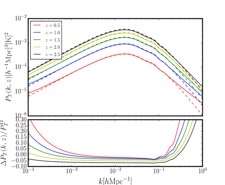
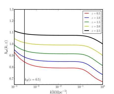
Figure 2: Left panel: Real space $P_{T}$ at five different redshifts $z=[0.5,1.0,1.5,2.0,2.5]$. Dashed lines are the linear theory result, while the thick lines include all the one-loop terms given in equations (56)-(58). In the lower left panel, we show the fractional difference (${\Delta P_{T}}/{P_{T}^{11}}={\big{[}P_{T}-P_{T}^{11}\big{]}}/{P_{T}^{11}}$). Right panel: Effective HI bias parameter from the uncorrected one-loop stochasticity in the auto power spectrum. It is defined in equation (67). We have normalized $b_{\rm{eff}}$ to remove dependence on $\bar{T}$. The dark vertical line indicates the horizon scale at $z=0.5$.

To obtain an effective HI bias parameter from $P_{T}$, one must quantify this term exactly and then subtract it off from the auto-power spectrum: $\sqrt{{(P_{T}(k)-S_{n})}/{P_{\delta\delta}(k)}}=b_{\text{eff}}^{T\delta}$ McDonald:2006mx ; McDonald:2009dh . It is only after this is done that a correspondence with the effective bias parameter from the cross-power spectrum between HI and matter over-densities(see equation (66)) agree. Figure2 shows that this spurious effect can induce a scale-dependence on the effective bias parameter that could mimic the signature of the primordial non-Gaussinity at low redshiftCamera:2013kpa .

IV.1.1 Stochastic power spectrum, shot noise and nonlinear effects

We shall now attempt to link the induced stochasticity due to nonlinear effects on small scales discussed in section IV.1 to the total noise budget for discrete tracers. We follow closely the definition of the stochastic power spectrum for any tracer given in Baldauf:2016sjb ; Baldauf:2013hka ; Hamaus:2010im . This definition assumes that on large scales, over-density is small hence linear local bias model is enough to relate a tracer to the underlying matter density field. The stochasticity in the tracer induces a power spectrum which may be defined as

$$(2\pi)^{3}\delta^{(\text{D})}\left({\bf{k}}+{\bf{k}}^{\prime}\right)C(k) = \langle\left(\delta_{\text{\tiny{HI}}}({\bf{k}})-b_{1}\delta_{m}({\bf{k}})\right)\left(\delta_{\text{\tiny{HI}}}({\bf{k}}^{\prime})-b_{1}\delta_{m}({\bf{k}}^{\prime})\right)\rangle$$ (69)

$$= (2\pi)^{3}\delta^{(\text{D})}\left({\bf{k}}+{\bf{k}}^{\prime}\right)\left[P_{T}(k)-2b_{1}P_{{}_{T\delta}}(k)+b_{1}^{2}P_{m}(k)\right]\,,$$ (70)

where $C(k)$ is the stochastic power spectrum at a given scale $k$, we have set $\bar{T}=1$ in this section in order to reduce clutter. For the local bias model, the linear bias parameter may be defined as $b_{1}=P_{T\delta}(k)/P_{m}(k)$ leading to the definition of the continuous HI power spectrum on large scales as

$$P_{T}^{\text{c}}(k) = C(k)+b_{1}^{2}P_{m}(k)\,.$$ (71)

What is observed/measured is not the continuous power spectrum given in equation (71) but the discrete tracer power spectrum(HI are resident in galaxies at low z and galaxies are discrete objects). For a finite number of discrete sources $N$, at position ${\bf{x}}$ in a finite volume $V$, the HI over-density in Fourier space is given by

$$\delta_{\text{\tiny{HI}}}({\bf{k}})=\frac{N}{V}\sum_{i}\exp\left[ikx_{i}\right]\,.$$ (72)

The power spectrum associated with the finite number of discrete sources may be defined as

$$P_{T}^{d}(k) = \frac{1}{V}\langle\delta_{\text{\tiny{HI}}}({\bf{k}})\delta_{\text{\tiny{HI}}}({\bf{k}}^{\prime})\rangle=\frac{V}{N^{2}}\left[\sum_{i=j}\langle\exp\left[ik(x_{i}-x_{j})\right]\rangle+\sum_{i\neq j}\langle\exp\left[ik(x_{i}-x_{j})\right]\rangle\right]$$ (73)

$$= P_{T}^{\text{shot}}+P_{{T}}^{\text{c}}(k)=P_{T}^{\text{shot}}+C(k)+b_{1}^{2}P_{m}(k)=S^{\rm eff}_{n}+b_{1}^{2}P_{m}(k)\,,$$ (74)

where $P_{T}^{\text{shot}}$ denotes the power spectrum associated with the shot noise and the non-zero separation part is identified with the continuous part of the discrete tracer power spectrum. In the second equality, we have replaced the continuous power spectrum with its definition given in equation(71) and in the third equality, we defined an effective noise parameter as a sum of the stochastic power spectrum and the intrinsic shot noise: $S^{\rm eff}_{n}=P_{T}^{\text{shot}}+S_{n}$. Here, $S_{n}$ is interpreted as an additional correction to the noise budget due to nonlinear mode couplingBaldauf:2016sjb . This is the rationale behind the identification of $S_{n}$ as shot noise inMcDonald:2006mx ; McDonald:2009dh .

We show in the right panel of figure 3 the effective or renormalized HI bias parameter(equation 66) assuming Sheth-Tormen model gives a fair estimate. In the left panel we show how it re-scales the power spectrum at one-loop order by computing the frame difference:

$$\Delta_{P_{T}}(k,z)=\frac{P_{T}(k,z)-S_{n}(z)-P^{11}_{T}(k,z)}{P^{11}_{T}(k,z)}\,.$$ (75)

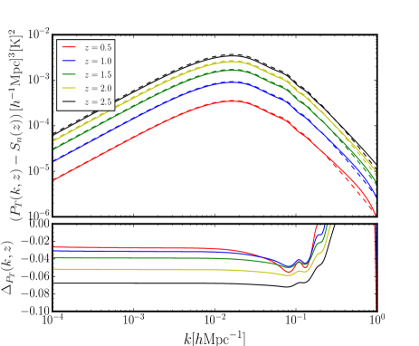
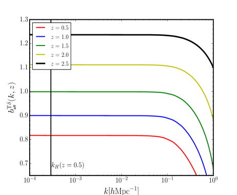
Figure 3: Left panel: Real space HI power spectrum with the stochastic power spectrum contribution subtracted off at five different redshifts $z=[0.5,1.0,1.5,2.0,2.5]$. In the lower left panel we show the fractional difference or the error associated with using the linear power spectrum instead of the full HI power spectrum. Right panel: Effective HI bias parameter defined in equation (66). We have normalized $b_{\rm{eff}}^{T\delta}$ to remove dependence on $\bar{T}$. The dark vertical line indicates the horizon scale at $z=0.5$.

There are two important consequences arising from equation (74) for $T^{\text{\tiny{obs}}}$ when nonlinear corrections are included in the analysis. These consequences are:

1. On large scales, nonlinear effects lead to an effective bias parameter which is different from the linear bias parameter estimated from the halo or HI mass function:

   $$b_{1}\mapsto b_{\text{eff}}^{T\delta}=b_{1}+\frac{1}{2}\left(b_{3}+\frac{68}{21}b_{2}\right)\sigma^{2}_{k\rm{nl}}\,,$$ (76)

   The terms in the bracket on the RHS are nonlinear bias parameters, multiplied by the matter variance. When the bias parameter is estimated from observation using the two-point correlation function, the measured value of the bias parameter will correspond to $b_{\text{eff}}^{T\delta}$ and not $b_{1}$.

2. Secondly, nonlinear effect induces a stochastic power spectrum which becomes important on large scales. The existence of the stochastic power spectrum indicates the break-down of perfect traceability by HI of the underlying matter density field.

Finally, in addition to $S_{n}^{\rm eff}$, the total power spectrum of the HI brightness temperature is also contaminated by the instrumental noise, galactic and extra-galactic foreground. However, most of the analysis of total power spectrum have so far neglected the contribution from $S_{n}^{\rm eff}$Bull:2014rha . The motivation for this is that the effect of $P_{T}^{\text{shot}}$ for the intensity mapping experiment is negligibleBull:2014rha ; Santos:2015gra ; Battye:2016qhf . It would be interesting to see whether the smallness of $P_{T}^{\text{shot}}$ also implies that $S_{n}^{\rm eff}$ is negligible. Following Bull:2014rha , $P_{T}^{\text{shot}}$ may be calculated from the comoving number density of haloes

$$P_{T}^{\text{shot}}=\left(\frac{\bar{T}(z)}{\rho_{\text{\tiny{HI}}}(z)}\right)^{2}\int_{M_{\rm{min}}}^{M_{\rm{max}}}\mbox{d}M\left[M_{\text{\tiny{HI}}}^{2}(M)n_{h}(z,M)\right]\,,$$ (77)

where $\rho_{\text{\tiny{HI}}}(z)$, $n_{h}$, $M_{\text{\tiny{HI}}}$ and the integral limits are defined in the appendix.

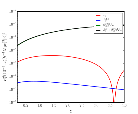
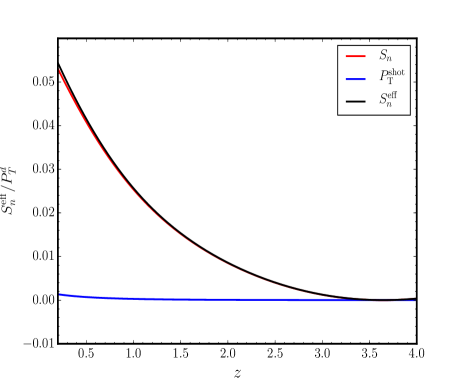
Figure 4: Left panel: Redshift evolution of the stochastic power spectrum, shot noise, the continuous power spectrum and discrete power spectrum. We set $k=10^{-3}h\rm{Mpc}^{-1}$. Right panel: The fractional contribution of the stochastic power spectrum and shot noise to the discrete power spectrum with $k$ set at $10^{-3}h\rm{Mpc}^{-1}$.

The renormalization procedure we have described provides a framework for interpreting the stochastic power spectrum as part of the total noise budget. We show in figure 4 that the contribution from $S_{n}$ is greater than that from $P_{T}^{\text{shot}}$ for the HI intensity mapping experiment. And that the effective shot noise contribution is dominated by $S_{n}$. The left panel shows that $S_{n}$ constitutes about 5% of discrete power spectrum at $z\leq 0.5$ and $k=10^{-3}h\rm{Mpc}^{-1}$. This is likely to have implications for the Fisher forecast analysis since the derivative of $S_{n}$ wrt the cosmological parameters is non-vanishing. Note that $S_{n}$ does not depend on any scale chosen to regulate the integral.

IV.2 HI power spectrum in redshift space

For the HI power spectrum in redshift space, we do not assume any phenomenological model for the FoG effect since our key interest is on the ultra-large scale features of the power spectrum. We show in figure 5 the relative contributions of ${P}_{T}^{11}$, ${P}_{T}^{22}$ and ${P}_{T}^{13}$ to the total radial power spectrum(top left panel) and transverse power spectrum(top right panel).

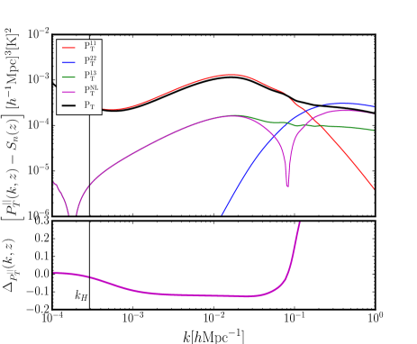
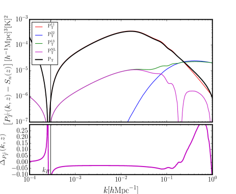
Figure 5: We show the radial ($P_{T}(k_{\parallel},z)=P^{||}_{T}(k,z)$) and transverse ($P_{T}(k_{\bot},z)=P^{\bot}_{T}(k,z)$ ) power spectrum at $z=0.5$ in the left and right panel respectively. The linear part of the transverse power spectrum goes to zero at about $k\sim k_{\mathcal{H}}$, this feature was first reported in Yoo:2010ni for the galaxy power spectrum. In the lower sections of each panel, we show the fractional difference between the total power spectrum and the linear theory prediction.

The plots show that in addition to the well-known imprint of nonlinear effects on the power spectrum on sub-horizon scales, the one-loop term gives a non-vanishing contribution on ultra-large scales, i.e $k\leq k_{\rm{eq}}$ through what may be considered as an additional correction to the bias parameter:

$$b_{\rm{eff}}^{T\delta}(k,\mu) \approx b_{1}+\frac{1}{2}\left[\left(b_{3}+\frac{68}{21}b_{2}\right)\sigma^{2}_{\Lambda}+\mathcal{I}_{R}(k,\mu)\right]\,.$$ (78)

The additional term, $\mathcal{I}_{R}$ is due to nonlinear redshift space distortions(see equation (54)). For $\mu=0$, we recover the real space effective HI bias parameter(see equation (66)). The fractional difference is weakly scale dependent in redshift space, this is due to the contribution from $\mathcal{I}_{R}$. This ultra-large scale dependent imprint of nonlinear effects is absent in the phenomenological models of the power spectrum in redshift space Scoccimarro:2004tg , since they assume a simple linear map of the galaxy over-density to the matter over-densityTaruya:2010mx .

In the lower panels of figure 5, we quantify the effective contribution of nonlinear effects to the power spectrum explicitly by computing the fractional difference. We show in the lower left panel of figure 5, that the error could be up to 12% on equality scale $k_{\rm{eq}}$. In the lower right panel of the same figure, we find about 5% correction for the orthogonal power spectrum, at $k_{\rm{eq}}$. The linear $P_{T}$ goes to zero on horizon scale, $k_{\mathcal{H}}$, this is due to vanishing of RSD and Doppler correction in the transverse direction. Therefore, the effective contribution is due to gravitational redshift term and $\delta_{\text{\tiny{HI}}}$ and the contribution from their cross correlation is negative in the neighbourhood of the horizon scales. In redshift space, the effective $P_{T}$ on large scales may be approximated by

$$P_{T}^{L}(k) \approx \bar{T}^{2}\bigg{\{}\left(b_{\rm{eff}}^{T\delta}(k,\mu)+f\mu^{2}+\mathcal{A}\,\frac{\mathcal{H}^{2}}{k^{2}}\right)^{2}+\mu^{2}\mathcal{B}^{2}\frac{\mathcal{H}^{2}}{k^{2}}\bigg{\}}P_{m}({k})+S_{n}\,.$$ (79)

Equation (79) reduces to equation (62) in the limit where all the light-cone projection effects are set to zero. On small scales, the product of two linear order RSD terms (Kaiser term) contained in $P^{22}_{T}$ is the dominant term:

$${P}_{T}^{22}({k},\mu) \approx \frac{\bar{T}^{2}}{2\pi^{2}}f^{2}\int_{k_{\rm{min}}}^{k_{\rm{max}}}{\mbox{d}k_{1}}\int_{-1}^{1}\mbox{d}\mu_{k}\bigg{[}k_{1}^{2}\bigg{|}\frac{\mu_{1}^{2}(k\mu-k_{1}\mu_{1})^{2}}{|{\bf{k}}-{\bf{k}}_{1}|^{2}}\bigg{|}^{2}P_{m}(|{\bf{k}}-{\bf{k}}_{1}|)P_{m}({k}_{1})\bigg{]}\,.$$ (80)

Equation (80) vanishes for $\mu=0$. We conclude this section by computing the monopole of the HI power spectrum

$$P^{0}_{T}(k) = (\bar{T})^{2}\bigg{[}b_{1}^{2}+\frac{2}{3}b_{1}f+\frac{1}{5}f^{2}+\frac{1}{3}\left[\mathcal{B}^{2}+2\left(3b_{1}+f\right)\mathcal{A}\right]\frac{\mathcal{H}^{2}}{k^{2}}+\mathcal{A}^{2}\frac{\mathcal{H}^{4}}{k^{4}}\bigg{]}P_{m}(k)+\frac{1}{2}\int_{-1}^{1}\mbox{d}\mu\,\left[{P}_{T}^{\rm{NL}}({k},\mu)\right]\,.$$ (81)

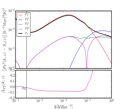
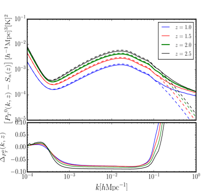
Figure 6: In the left panel, we show the monopole of the total power spectrum of the HI brightness temperature in redshift space at $z=0.5$. One the right panel, we show the monopole of the power spectrum of $T\text{\tiny{obs}}$ at $z=1.0$ (blue curve), $z=1.5$ (red curve), $z=2.0$ (green curve) and $z=2.5$ (black curve). The dashed lines indicate the linear theory prediction. The fractional difference is shown in the bottom panels.

At $z=0.5$, there is about 7% modulation in the amplitude of the monopole of $P_{T}$ by nonlinear effects on large scales. The effective contribution drops to less than 2% at the horizon scale. In the right panel of figure 6, we show the redshift dependence of nonlinear effects on the power spectrum. The magnitude of the nonlinear correction increases slightly as the redshift increases. This feature is due to the redshift evolution of the bias parameters. We summarise the imprints of nonlinear effects in the bias and nonlinear RSD on$P_{T}$ on all scales in Table 1. We did not calculate the effective HI bias in redshift space in a similar way as we did in real space, this will be pursued in a future work since it will require the monopole of the matter power spectrum in redshift space which is beyond the scope of this work.

$P_{T}(k)$	$k_{\mathcal{H}}\leq k\leq k_{\rm{eq}}$	$k_{\rm{eq}}\leq k\leq k_{\rm{BAO}}^{\rm{end}}$	$k>k_{\rm{BAO}}^{\rm{end}}$
$P_{T}^{\|}(k)$	$1\,\leq$ $\Delta\leq\,$ 12	12 $\leq$ $\Delta\leq\,30$	$\Delta>30$
$P_{T}^{\bot}(k)$	$10$ $\leq$ $\Delta\leq\,$5	5 $\leq$ $\Delta\leq\,$5	$\Delta>10$
$P_{T}^{0}(k)$	$1\,\leq$ $\Delta\leq\,7$	$7\leq$ $\Delta\leq\,30$	$\Delta>30$

Table 1: Summary of the imprint of nonlinear effects in the bias and nonlinear RSD on HI power spectrum in redshift space at $z=0.5$. $\Delta$ corresponds to the percentage error associated with using linear theory approximation to calculate the HI power spectrum. We defined $k_{\rm{BAO}}^{\rm{end}}\approx 0.3\,h\rm{Mpc}^{-1}$. Predictions of the standard perturbation theory at one-loop level may not be trusted beyond $k_{\rm{BAO}}$ at $z=0.5$.

V Conclusion

In this paper, we have studied in detail, how nonlinearity in the bias and peculiar velocity could modulate clustering of HI brightness temperature on large scales. We approached the problem by using the general relativistic perturbation theory techniques to derive for the first time, the full nonlinear expression for the HI brightness temperature up to third order in perturbation theory in the post-re-ionization universe. The full expression we derived, describes how weak gravitational lensing, redshift space distortions induced by the peculiar velocity, gravitational redshift, ISW and HI bias affect the clustering of the HI brightness temperature. When we take the plane-parallel approximation, we recover exactly the previous results that made use of a different technique to derive the corresponding expression for the galaxy number count in the Newtonian limitBernardeau:2001qr ; Heavens:1998es .

Our expression for the perturbed HI brightness temperature includes contributions from: the Sachs-Wolfe effect(gravitational redshift correction), Integrated Sachs-Wolfe effects(contribution due to evolving gravitational potential along the line of sight), Doppler effects(effect due to relative motion of the source and the observer), Kaiser effect(linear RSD), nonlinear RSD (FoG effect) and weak gravitational lensing. We introduced the HI bias after transforming the HI over-density to the comoving synchronous gauge, then use simple local Eulerian bias model expanded up to third order in perturbation theory to relate it to the underlying dark matter density field. The HI bias parameters were calculated from the halo model using Sheth-Torman halo mass functionSheth:2001dp . We allowed non-Gaussianity in the bias only in the linear order perturbation of HI number density, since its influence on the bias is sub-dominant at one-loop level. The signal from non-Gaussianity in the matter density field is also sub-dominant at power spectrum level, hence we neglected it as well.

We calculate the real space power spectrum of the HI brightness temperature at four different redshift points. We use a bias renormalization prescription presented in McDonald:2009dh to renormalize FLRW background number density of HI atoms and the brightness temperature. The auto power spectrum of the HI bias parameter at second order leads to a white noise-like contribution on large scales, this contribution may be treated as part of the effective shot noise contribution. We also calculate the redshift space power spectrum of the HI brightness temperature. We show that, in addition to nonlinear effects contributing significantly to the power spectrum on small scales, it also modulates the power spectrum on large scales due to mode coupling at nonlinear order. We show that on scales $k\leq k_{\rm{eq}}$, $P_{T}$ receives a cut-off dependent correction from nonlinear effects in the bias and nonlinear RSD.

Finally, all the results we presented on modulation of the HI power spectrum on large scales by nonlinear effects is dependent on the cut-off chosen to regulate the convolution integrals in $P^{13}_{T}$. We adopted a simple regularisation technique which suppresses modes greater than $k_{\rm{nl}}$. This cut-off is chosen to ensure that we remain within the regime of validity of the cosmological perturbation theorySmith:2002dz . A more rigorous treatment will involve adopting a renormalization procedure that could eliminate the dependence of the result on a cut-off scaleBaldauf:2014qfa . Also, we used a simple Sheth-Tormen halo mass functionSheth:1999mn and a polynomial fit for the HI mass profile to estimate all the HI bias parameters. A more accurate model for the HI mass would be needed for a more accurate quantitative treatmentPadmanabhan:2016fgy ; Padmanabhan:2016odj .

Appendix A Basic cosmological perturbation theory

Here we provide more details on the perturbation theory calculation up to third order, using the approach developed in Umeh:2012pn ; Umeh:2014ana . We consider a perturbed FLRW spacetime in the Poisson gauge assuming a conformally flat background metric

$$\mbox{d}s^{2}=a^{2}\left[-(1+2\Phi+\Phi^{\text{\tiny({{2}})}}+\frac{1}{3}\Phi^{\text{\tiny({{3})}}})\mbox{d}\eta^{2}+\left((1-2\Psi-\Psi^{\text{\tiny({{2}})}}-\frac{1}{3}\Psi^{\text{\tiny({{3})}}})\delta_{ij}\right)\mbox{d}x^{i}\mbox{d}x^{j}\right]\,.$$ (82)

Here the proper time is related to conformal time by $\mbox{d}t=a\mbox{d}\eta$. $\Phi$ is the first-order Newtonian gravitational potential, $\Psi$ is scalar curvature perturbation. For any tensor $S$ we expand it up to third order as

$$\hat{S}=\bar{S}+\delta^{\text{\tiny({1})}}S+\frac{1}{2}\delta^{\text{\tiny({{2}})}}S+\frac{1}{3!}\delta^{\text{\tiny({{3})}}}S\,.$$ (83)

We expand the 4-velocity $u^{a}$, of a matter field using (82) up to third order

$$u^{0} = 1-\Phi+\frac{1}{2}\left[3\Phi^{2}-\Phi^{\text{\tiny({{2}})}}+{\partial}_{i}v{\partial}^{i}v\right]+\frac{1}{3!}\bigg{[}-\Phi^{\text{\tiny({{3})}}}-15\Phi^{3}+9\Phi\Phi^{\text{\tiny({{2}})}}+3{v^{\text{\tiny({{2}})}}}^{i}{\partial}_{i}v-3\Phi{\partial}_{i}v{\partial}^{i}v$$

$$-6\Psi{\partial}_{i}v{\partial}^{i}v+3{\partial}_{i}v^{\text{\tiny({{2}})}}{\partial}^{i}v\bigg{]}\,,$$

$$u^{i} = {\partial}^{i}v+\frac{1}{2}\left[v^{i}{}^{\text{\tiny({{2}})}}+{\partial}^{i}v^{\text{\tiny({{2}})}}\right]+\frac{1}{3!}\left[v^{i}{}^{\text{\tiny({{3})}}}+{\partial}^{i}v^{\text{\tiny({{3})}}}\right]\,.$$ (85)

In cosmological perturbation theory, the map between real and redshift space is given by $s^{i}=x^{i}+\Delta^{\text{\tiny({1})}}x^{i}+\Delta^{\text{\tiny({{2}})}}x^{i}/2+\Delta^{\text{\tiny({{3})}}}x^{i}/3!$, where

$$\Delta^{\text{\tiny({1})}}x^{i} = \overbrace{\delta^{\text{\tiny({1})}}x^{i}_{\bot}}^{\Delta^{\text{\tiny({1})}}x_{\bot}}+n^{i}\overbrace{\left(\delta^{\text{\tiny({1})}}x_{{\text{\tiny$\|$}}}+\frac{\delta^{\text{\tiny({1})}}z}{\mathcal{H}_{s}}\right)}^{\Delta^{\text{\tiny({1})}}x_{{\text{\tiny$\|$}}}}\approx\delta^{\text{\tiny({1})}}x^{i}_{\bot}+n^{i}\frac{\delta^{\text{\tiny({1})}}z}{\mathcal{H}_{s}}\,.$$ (86)

Here, we have considered only the dominant terms in the second equality. In the plane-parallel limit the dominant term is given by

$$\Delta^{\text{\tiny({1})}}x^{i} \approx n^{i}\frac{\delta^{\text{\tiny({1})}}z}{\mathcal{H}_{s}}=-n^{i}\frac{1}{\mathcal{H}_{s}}\nabla_{{}_{{\text{\tiny$\|$}}}}v_{s}^{\text{\tiny({1})}}\,.$$ (87)

We have considered only the radial component of the peculiar velocity. The second order correction to the real to redshift space map is given by

$$\Delta^{\text{\tiny({{2}})}}x^{i} = \delta^{\text{\tiny({{2}})}}x^{i}_{\bot}-\frac{2}{\mathcal{H}_{s}}\delta^{\text{\tiny({1})}}x^{\prime}_{\bot}{}^{i}\delta^{\text{\tiny({1})}}z+2\Delta^{\text{\tiny({1})}}x_{{\text{\tiny$\|$}}}\nabla_{{\text{\tiny$\|$}}}\delta^{\text{\tiny({1})}}x^{i}_{\bot}+2\Delta^{\text{\tiny({1})}}x^{i}_{\bot}\nabla_{\bot j}\delta^{\text{\tiny({1})}}x^{i}_{\bot}$$

$$+n^{i}\bigg{[}\delta^{\text{\tiny({{2}})}}x_{{\text{\tiny$\|$}}}+\frac{\delta^{\text{\tiny({{2}})}}z}{\mathcal{H}_{s}}-2\frac{\delta^{\text{\tiny({1})}}z}{\mathcal{H}_{s}}\left(\delta^{\text{\tiny({1})}}x_{{\text{\tiny$\|$}}}^{\prime}+\frac{\delta^{\text{\tiny({1})}}z^{\prime}}{\mathcal{H}_{s}}\right)+2\Delta^{\text{\tiny({1})}}x_{{\text{\tiny$\|$}}}\left(\nabla_{{\text{\tiny$\|$}}}\delta^{\text{\tiny({1})}}x_{{\text{\tiny$\|$}}}+\frac{\nabla_{{\text{\tiny$\|$}}}\delta^{\text{\tiny({1})}}z}{\mathcal{H}}\right)$$

$$+2\Delta^{\text{\tiny({1})}}x^{j}_{\bot}\left(\nabla_{\bot j}\delta^{\text{\tiny({1})}}x_{{\text{\tiny$\|$}}}+\frac{\nabla_{\bot j}\delta^{\text{\tiny({1})}}z}{\mathcal{H}_{s}}\right)-\frac{2}{\chi}\delta^{\text{\tiny({1})}}x^{k}_{\bot}\Delta^{\text{\tiny({1})}}x_{\bot k}-\frac{(\delta^{\text{\tiny({1})}}z)^{2}}{\mathcal{H}_{s}}\left(1+\frac{\mathcal{H}^{\prime}_{s}}{\mathcal{H}_{s}^{2}}\right)\bigg{]}$$

$$\approx \overbrace{\delta^{\text{\tiny({{2}})}}x^{i}_{\bot}+2\Delta^{\text{\tiny({1})}}x^{j}_{\bot}\nabla_{\bot j}\delta^{\text{\tiny({1})}}x^{i}_{\bot}}^{\Delta^{\text{\tiny({{2}})}}x_{\bot}}+\frac{n^{i}}{\mathcal{H}_{s}}\overbrace{\left[\delta^{\text{\tiny({{2}})}}z+2\left(\Delta^{\text{\tiny({1})}}x_{{\text{\tiny$\|$}}}\nabla_{{\text{\tiny$\|$}}}\delta^{\text{\tiny({1})}}z+\Delta^{\text{\tiny({1})}}x^{j}_{\bot}\nabla_{\bot j}\delta^{\text{\tiny({1})}}z\right)\right]}^{\Delta^{\text{\tiny({{2}})}}x_{{\text{\tiny$\|$}}}}\,,$$ (89)

where the approximation sign shows the limit of approximation used in the paper. The radial component becomes

$$\Delta^{\text{\tiny({{2}})}}x_{{\text{\tiny$\|$}}} \approx \frac{n^{i}}{\mathcal{H}_{s}}\left[\delta^{\text{\tiny({{2}})}}z+2\left(\Delta^{\text{\tiny({1})}}x_{{\text{\tiny$\|$}}}\nabla_{{\text{\tiny$\|$}}}\delta^{\text{\tiny({1})}}z+\Delta^{\text{\tiny({1})}}x^{j}_{\bot}\nabla_{\bot j}\delta^{\text{\tiny({1})}}z\right)\right]\,,$$ (90)

$$\approx n^{i}\left[-\frac{1}{\mathcal{H}_{s}}\nabla_{{}_{{\text{\tiny$\|$}}}}v_{s}^{\text{\tiny({{2}})}}+2\left[\frac{1}{\mathcal{H}_{s}^{2}}\nabla_{{}_{{\text{\tiny$\|$}}}}v_{s}^{\text{\tiny({1})}}\nabla_{{}_{{\text{\tiny$\|$}}}}^{2}v_{s}^{\text{\tiny({1})}}-\frac{1}{\mathcal{H}_{s}}\nabla_{\bot j}\nabla_{{}_{{\text{\tiny$\|$}}}}v_{s}\int^{\chi_{s}}_{0}\frac{(\chi-\chi_{s})}{\chi_{s}}\nabla_{\bot}^{j}\Phi_{A}^{\text{\tiny({1})}}\mbox{d}\chi\right]\right]\,,$$ (91)

The terms in the square bracket in the second equality are Post-Born terms. The covariant derivatives which appear after implementing Born and Post-Born correction to the fluctuation of the HI brightness temperature are decomposed as follows:

$$\Delta^{\text{\tiny({1})}}x^{a}\nabla_{a}\delta^{\text{\tiny({1})}}T = \frac{\delta^{\text{\tiny({1})}}z}{\mathcal{H}_{s}}{\delta^{\text{\tiny({1})}}{T}}^{\prime}+\Delta^{\text{\tiny({1})}}x_{{}_{{\text{\tiny$\|$}}}}\nabla_{{}_{{\text{\tiny$\|$}}}}\delta^{\text{\tiny({1})}}{T}+\Delta^{\text{\tiny({1})}}x_{\bot}^{i}\nabla_{\bot i}\delta^{\text{\tiny({1})}}{T}\,,$$ (92)

$$\approx \Delta^{\text{\tiny({1})}}x_{{}_{{\text{\tiny$\|$}}}}\nabla_{{}_{{\text{\tiny$\|$}}}}\delta^{\text{\tiny({1})}}{T}+\Delta^{\text{\tiny({1})}}x_{\bot}^{i}\nabla_{\bot i}\delta^{\text{\tiny({1})}}{T}\,,$$ (93)

where $\Delta^{\text{\tiny({1})}}x_{{}_{{\text{\tiny$\|$}}}}$ and $\Delta^{\text{\tiny({1})}}x_{\bot}^{i}$ are given in equation (86). For double covariant derivatives we decompose as follows:

$$\Delta^{\text{\tiny({1})}}x^{a}\Delta^{\text{\tiny({1})}}x^{b}\nabla_{a}\nabla_{b}\delta^{\text{\tiny({1})}}T = (\delta^{\text{\tiny({1})}}\lambda)^{2}{\delta^{\text{\tiny({1})}}T}^{\prime\prime}-2\delta^{\text{\tiny({1})}}\lambda\Delta^{\text{\tiny({1})}}x_{{\text{\tiny$\|$}}}\nabla_{{\text{\tiny$\|$}}}{\delta^{\text{\tiny({1})}}T}^{\prime}+(\Delta^{\text{\tiny({1})}}x_{{\text{\tiny$\|$}}})^{2}{\nabla_{{\text{\tiny$\|$}}}}^{2}{\delta^{\text{\tiny({1})}}T}$$

$$+\frac{1}{\chi_{s}}\Delta^{\text{\tiny({1})}}{x_{\bot}}_{i}\Delta^{\text{\tiny({1})}}{x_{\bot}}^{i}\nabla_{{\text{\tiny$\|$}}}{\delta^{\text{\tiny({1})}}T}-\frac{2}{\chi_{s}}\Delta^{\text{\tiny({1})}}x_{{\text{\tiny$\|$}}}\Delta^{\text{\tiny({1})}}{x_{\bot}}^{i}\nabla_{\bot i}\delta^{\text{\tiny({1})}}T+2\Delta^{\text{\tiny({1})}}x_{{\text{\tiny$\|$}}}\Delta^{\text{\tiny({1})}}{x_{\bot}}^{i}\nabla_{\bot i}\nabla_{{\text{\tiny$\|$}}}\delta^{\text{\tiny({1})}}T$$

$$+2\delta^{\text{\tiny({1})}}\lambda\Delta^{\text{\tiny({1})}}{x_{\bot}}^{i}\nabla_{\bot i}{\delta^{\text{\tiny({1})}}T}^{\prime}+\Delta^{\text{\tiny({1})}}{x_{\bot}}^{i}\Delta^{\text{\tiny({1})}}{x_{\bot}}^{j}\nabla_{\bot i}\nabla_{\bot j}{\delta^{\text{\tiny({1})}}T}\,,$$

$$\approx (\Delta^{\text{\tiny({1})}}x_{{\text{\tiny$\|$}}})^{2}\nabla_{{\text{\tiny$\|$}}}^{2}\delta^{\text{\tiny({1})}}T+2\Delta^{\text{\tiny({1})}}x_{{\text{\tiny$\|$}}}\Delta^{\text{\tiny({1})}}{x_{\bot}}^{i}\nabla_{\bot i}\nabla_{{\text{\tiny$\|$}}}\delta^{\text{\tiny({1})}}T+\Delta^{\text{\tiny({1})}}{x_{\bot}}^{i}\Delta^{\text{\tiny({1})}}{x_{\bot}}^{j}\nabla_{\bot i}\nabla_{\bot j}{\delta^{\text{\tiny({1})}}T}\,,$$ (95)

where in the second equality, we have considered only the dominant part. We have twice projected screen space derivatives, we expand them in Fourier space by first expressing them in terms of the spatial derivatives

$$\nabla_{\bot}^{2} = \nabla_{i}\nabla^{i}-\nabla_{{\text{\tiny$\|$}}}^{2}-\frac{2}{\chi}\nabla_{{\text{\tiny$\|$}}}\approx\nabla_{i}\nabla^{i}-\nabla_{{\text{\tiny$\|$}}}^{2}\,,$$ (96)

$$\nabla_{\bot i}\nabla_{\bot j} = \nabla_{i}\nabla_{j}-n_{i}n_{j}\nabla^{2}_{{\text{\tiny$\|$}}}-2n_{(i}\nabla_{{\text{\tiny$\|$}}}\nabla_{\bot j)}-\frac{1}{2\chi}N_{ij}\nabla_{{\text{\tiny$\|$}}}+\frac{1}{\chi}n_{(i}\nabla_{\bot j)}\approx\nabla_{i}\nabla_{j}-n_{i}n_{j}\nabla^{2}_{{\text{\tiny$\|$}}}-2n_{(i}\nabla_{{\text{\tiny$\|$}}}\nabla_{\bot j)}\,.$$ (97)

And for once projected screen space derivative and derivative along the line of sight we have

$$\nabla_{{\text{\tiny$\|$}}}=n^{i}\nabla_{i}\,,\quad\nabla^{2}_{{\text{\tiny$\|$}}}=\nabla_{{\text{\tiny$\|$}}}\nabla_{{\text{\tiny$\|$}}}\,,\quad\nabla_{\bot i}=N_{i}{}^{j}\nabla_{j}=\nabla_{i}-n_{i}\nabla_{{\text{\tiny$\|$}}}\,,\quad\nabla_{i}n^{j}=\frac{1}{\chi}N^{j}{}_{i}$$ (98)

Appendix B Standard Dark matter perturbation theory

The solutions for the $n$-th order solution for a coupled dark matter over-density $\delta_{\text{m}}$ and velocity divergence, $\theta({\bf{k}})$ equation are given by Bernardeau:2001qr :

$$\delta_{\text{m}}({\bf{k}})=\sum_{n=1}^{\infty}\delta_{\text{m}}^{(n)}({\bf{k}}), \theta({\bf{k}})=-\mathcal{H}f\sum_{n=1}^{\infty}\theta^{(n)}({\bf{k}})\,.$$ (99)

At $n$-th order we have

$$\delta_{\text{m}}^{(n)}({\bf{k}})=\int\frac{d^{3}k_{1}}{(2\pi)^{3}}\ldots\int\frac{d^{3}k_{n}}{(2\pi)^{3}}\delta_{\text{m}}({\bf{k}}_{1})\ldots\delta_{\text{m}}({\bf{k}}_{n})F_{n}({\bf{k}}_{1},\ldots,{\bf{q}}_{n})\delta^{\text{(D)}}({\bf{q}}_{1}+\ldots+{\bf{k}}_{n}-{\bf{k}})\,,$$ (100)

$$\theta^{(n)}({\bf{k}})=\int\frac{d^{3}k_{1}}{(2\pi)^{3}}\ldots\int\frac{d^{3}k_{n}}{(2\pi)^{3}}\delta_{\text{m}}({\bf{k}}_{1})\ldots\delta_{\text{m}}({\bf{k}}_{n})G_{n}({\bf{k}}_{1},\ldots,{\bf{k}}_{n})\delta^{\text{(D)}}({\bf{k}}_{1}+\ldots+{\bf{k}}_{n}-{\bf{k}}),$$ (101)

where the coupling kernels $F_{n}$ and $G_{n}$ can be obtained using recursion relations.

$${F}_{2}({\bf{k}}_{1},{\bf{k}}_{2}) = {5\over 7}+{{\bf{k}}_{1}\cdot{\bf{k}}_{2}\over 2k_{1}k_{2}}\left({k_{1}\over k_{2}}+{k_{2}\over k_{1}}\right)+{2\over 7}\left({{\bf{k}}_{1}\cdot{\bf{k}}_{2}\over k_{1}k_{2}}\right)^{2},$$ (102)

$${G}_{2}({\bf{k}}_{1},{\bf{k}}_{2}) = {3\over 7}+{{\bf{k}}_{1}\cdot{\bf{k}}_{2}\over 2k_{1}k_{2}}\left({k_{1}\over k_{2}}+{k_{2}\over k_{1}}\right)+{4\over 7}\left({{\bf{k}}_{1}\cdot{\bf{k}}_{2}\over k_{1}k_{2}}\right)^{2},$$ (103)

$${F}_{3}^{s}({\bf{k}}_{1},{\bf{k}}_{2},{\bf{k}}_{3}) = F_{2}({\bf{k}}_{2},{\bf{k}}_{3})\left[{1\over 3}+{1\over 3}{{\bf{k}}_{1}\cdot({\bf{k}}_{2}+{\bf{k}}_{3})\over({\bf{k}}_{2}+{\bf{k}}_{3})^{2}}+{4\over 9}{{\bf{k}}\cdot{\bf{k}}_{1}\over k_{1}^{2}}{{\bf{k}}\cdot({\bf{k}}_{2}+{\bf{k}}_{3})\over({\bf{k}}_{2}+{\bf{k}}_{3})^{2}}\right]$$

$$-{2\over 9}{{\bf{k}}\cdot{\bf{k}}_{1}\over k_{1}^{2}}{{\bf{k}}\cdot({\bf{k}}_{2}+{\bf{k}}_{3})\over({\bf{k}}_{2}+{\bf{k}}_{3})^{2}}{{\bf{k}}_{3}\cdot({\bf{k}}_{2}+{\bf{k}}_{3})\over k_{3}^{2}}+{1\over 9}{{\bf{k}}\cdot{\bf{k}}_{2}\over k_{2}^{2}}{{\bf{k}}\cdot{\bf{k}}_{3}\over k_{3}^{2}}\,,$$

$${G}_{3}^{s}({\bf{k}}_{1},{\bf{k}}_{2},{\bf{k}}_{3}) = 3F_{3}^{s}({\bf{k}}_{1},{\bf{k}}_{2},{\bf{k}}_{3})-{{\bf{k}}\cdot{\bf{k}}_{1}\over k_{1}^{2}}F_{2}({\bf{k}}_{2},{\bf{k}}_{3})-{{\bf{k}}\cdot({\bf{k}}_{1}+{\bf{k}}_{2})\over({\bf{k}}_{1}+{\bf{k}}_{2})^{2}}G_{2}({\bf{k}}_{1},{\bf{k}}_{2}),$$ (105)

with ${\bf{k}}={\bf{k}}_{1}+{\bf{k}}_{2}+{\bf{k}}_{3}$ in the last two expressions. The subscript $S$ indicates that the expression has been made symmetric w.r.t. any permutation of the arguments. We normalized the dark matter kernels appropriately to agree with the coefficient of our Taylor expansion. The matter power spectrum up to one-loop correction is given by

$${P}_{\delta\delta}(k) = P_{m}(k)+P^{22}_{\delta\delta}(k)+P^{13}_{\delta\delta}(k)\,,$$ (106)

where $P_{m}(k)$ is the standard linear dark matter power spectrum and other one-loop correction terms are given by

$$P^{22}_{\delta\delta}(k) = \frac{1}{2}\int\frac{\mathrm{d}^{3}k_{1}}{(2\pi)^{3}}P_{m}(k_{1})P_{m}(\left|{\bf{k}}-{\bf{k}}_{1}\right|)\left|F_{2}({\bf{k}}_{1},{\bf{k}}-{\bf{k}}_{1})\right|^{2}\,,$$ (107)

$$P^{13}_{\delta\delta}(k) = \frac{1}{252}\frac{k^{3}}{4\pi^{2}}P_{m}(k)\int_{0}^{\infty}dr~{}P_{m}(kr)\left[\frac{12}{r^{2}}-158+100r^{2}-42r^{4}+\frac{3}{r^{3}}(r^{2}-1)^{3}(7r^{2}+2)\ln\left|\frac{1+r}{1-r}\right|\right]\,.$$ (108)

Similarly, for the peculiar velocity term, we have

$${P}_{\theta\theta}(k) = P_{m}(k)+P^{22}_{\theta\theta}(k)+P^{13}_{\theta\theta}(k)\,,$$ (109)

where $P^{22}_{\theta\theta}(k)$ and $P^{13}_{\theta\theta}(k)$ take similar forms as in equation (107).

$$P^{22}_{\theta\theta}(k) = \frac{1}{2}\int\frac{\mathrm{d}^{3}k_{1}}{(2\pi)^{3}}P_{m}(k_{1})P_{m}^{11}(\left|{\bf{k}}-{\bf{k}}_{1}\right|)\left|G_{2}({\bf{k}}_{1},{\bf{k}}-{\bf{k}}_{1})\right|^{2}\,,$$ (110)

$$P^{13}_{\theta\theta}(k) = \frac{1}{84}\frac{k^{3}}{4\pi^{2}}P_{m}(k)\int_{0}^{\infty}dr~{}P_{m}(kr)\left[\frac{12}{r^{2}}-82+4r^{2}-6r^{4}+\frac{3}{r^{3}}(r^{2}-1)^{3}(r^{2}+2)\ln\left|\frac{1+r}{1-r}\right|\right]\,.$$ (111)

The integrands introduced in equation (55) are Matsubara:2007wj ; Donghui2010

$$B_{1101}(r) = \frac{1}{2}\ ,$$ (112)

$$B_{1110}(r) = \frac{1}{84}\left[-2\left(9r^{4}-24r^{2}+19\right)+\frac{9}{r}\left(r^{2}-1\right)^{3}\ln\left(\frac{1+r}{|1-r|}\right)\right]\,,$$ (113)

$$B_{1210}(r) = -\frac{1}{3}\,,$$ (114)

$$B_{1200}(r) = -\frac{1}{336r^{3}}\left[2\left(-9r^{7}+33r^{5}+33r^{3}-9r\right)+9\left(r^{2}-1\right)^{4}\ln\left(\frac{1+r}{|1-r|}\right)\right]\,,$$ (115)

$$B_{2220}(r) = \frac{1}{336r^{3}}\left[2r\left(-27r^{6}+63r^{4}-109r^{2}+9\right)+9\left(3r^{2}+1\right)\left(r^{2}-1\right)^{3}\ln\left(\frac{1+r}{|1-r|}\right)\right]\,,$$ (116)

$$B_{2300}(r) = -\frac{1}{3}\,.$$ (117)

Appendix C How we obtain HI bias from halo bias

We calculate the bias parameters from a simple Sheth-Torman halos mass function for a spherical collpase model Sheth:1999mn :

$$n_{h}(M)=\nu f(\nu)\frac{\bar{\rho}}{M^{2}}\frac{\mbox{d}\ln\nu}{\mbox{d}\ln M},$$ (118)

where the peak height $\nu$ is related to the variance in dark matter density field, $\sigma^{2}$, $\nu=(\delta_{c}/\sigma_{nG})^{2}$ and $\delta_{c}=1.686$ is the critical threshold for a spherical collapse at the current epoch obtained from linear perturbation theory. A halo of mass $M=\bar{\rho}V$ is formed when the walk first crosses a barrier $f(\nu)$:

$$\nu f(\nu)=A(p)\left(1+\frac{1}{(q\nu)^{p}}\right)\sqrt{\frac{q\nu}{2\pi}}\left[-\frac{q\nu}{2}\right],$$ (119)

where $q=0.707$ and $p=0.3$ are obtained from a fit to numerical simulations. A similar model exists for ellipsoidal collapse Sheth:2001dp .

$$b_{1} = 1+\left\langle\frac{(q\nu-1)}{\delta_{c}}+\frac{2p}{\delta_{c}\left(1+(q\nu)^{p}\right)}\right\rangle_{\tiny{\text{M}}}\,,$$ (120)

$$b_{2} = \frac{8}{21}\left(b_{1}-1\right)+\left\langle\frac{4\left(p^{2}+\nu pq\right)-(q\nu-1)\left(1+(q\nu)^{p}\right)-2p}{\delta^{2}_{c}\left(1+(q\nu)^{p}\right)}+\frac{1}{\delta_{c}^{2}}\left((q\nu)^{2}-2q\nu-1\right)\right\rangle_{\tiny{\text{M}}}\,$$ (121)

$$b_{3} = -\frac{236}{189}\left(b_{1}-1\right)-\frac{13}{7}\left(b_{2}-\frac{8}{21}\left(b_{1}-1\right)\right)+\bigg{<}-\frac{\left(3+3\nu q+3\nu^{2}q^{2}-\nu^{3}q^{3}\right)}{\delta_{c}^{3}}$$

$$+\frac{\left(8p^{3}+12p^{2}\left(1+\nu q\right)+p\left(6\nu^{2}q^{2}-2\right)\right)}{\delta_{c}^{3}\left(1+1+(\nu q)^{p}\right)}+6\frac{\left(1+2\nu q-\nu^{2}q^{2}\right)}{\delta_{c}^{3}}-24\frac{\left(p^{2}+\nu pq\right)}{\delta_{c}^{3}\left(1+(\nu q)^{p}\right)}$$

$$-4\frac{(1-\nu q)}{\delta_{c}^{3}}+8\frac{p}{\delta_{c}^{3}\left(1+(q\nu)^{p}\right)}\bigg{>}_{\rm M}\,,$$

The HI bias parameters used in the paper were obtained by averaging over the halo bias parameters according to

$$X(z,{\bf{x}})=\left\langle X_{h}(z,{\bf{x}})\right\rangle_{\tiny{\text{M}}}=\frac{\int_{M_{\rm{min}}}^{M_{\rm{max}}}\mbox{d}M\left[X_{h}(z,{\bf{x}},M)M_{\text{\tiny{HI}}}(M)n_{h}(z,{\bf{x}},M)\right]}{\int_{M_{\rm{min}}}^{M_{\rm{max}}}\mbox{d}M\left[M_{\text{\tiny{HI}}}(M)n_{h}(z,{\bf{x}},M)\right],}$$ (123)

where $M_{\rm{min}}$ and $M_{\rm{max}}$ are the lower and upper limits of masses, which are related to the limits of circular velocity of galaxies that could house HI. These are obtained from the circular velocity constraint

$$v_{\text{circ}}=30\sqrt{1+z}\left(\frac{M}{10^{10}M_{\odot}}\right)^{1/3}~{}{\rm km\,s}^{-1}\,,$$ (124)

We assumed that only halos with circular velocities between $30-200\,$kms^-1 are able to host HI. This range of circular velocity is motivated by observation Bull:2014rha . We adopt a simple polynomial fitting function for the HI mass function. This choice is based on the results from an N-body simulation for the HI mass function Santos:2015gra

$$M_{\text{\tiny{HI}}}(M)=CM^{0.6}\,,$$ (125)

Here, the normalization factor is chosen to match the measurement of $\Omega_{\text{\tiny{HI}}}$ at $z=0.8$ Switzer:2013ewa . We compute each of the bias parameters in figure 7.

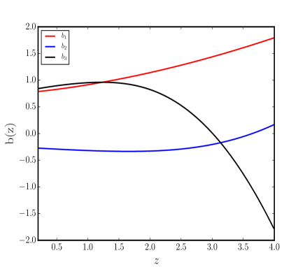
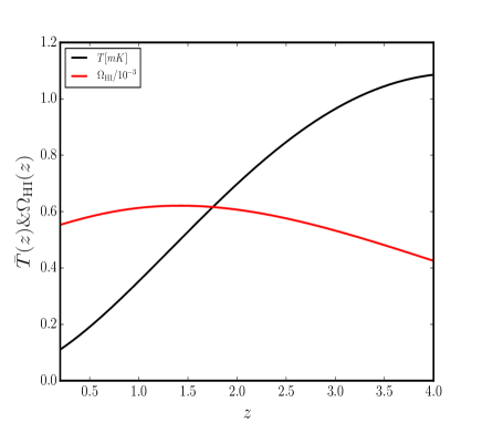
Figure 7: Left panel: The HI bias parameters constructed from Sheth-Torman halos mass function. Right panel: Redshift evolution of the mean HI brightness temperature and HI density parameter.

The $\Omega_{\text{\tiny{HI}}}$ at any redshift may also be obtained from the halo model

$$\Omega_{\text{\tiny{HI}}}(z)\equiv\dfrac{1}{(1+z)^{2}}\frac{\rho_{\text{\tiny{HI}}}(z)}{\rho_{c,0}}\,,$$ (126)

where $\rho_{c,0}$ is the homogeneous matter density today and $\rho_{\text{\tiny{HI}}}$ is the density of the HI atoms

$$\rho_{\text{\tiny{HI}}}(z)=\int_{M_{\rm{min}}}^{M_{\rm{max}}}\mbox{d}M\left[M_{\text{\tiny{HI}}}(M)n_{h}(z,M)\right]\,.$$ (127)

References

• (1) P. Bull, P. G. Ferreira, P. Patel, and M. G. Santos, Late-time cosmology with 21cm intensity mapping experiments, arXiv:1405.1452.
• (2) J. Fonseca, S. Camera, M. Santos, and R. Maartens, Hunting down horizon-scale effects with multi-wavelength surveys, arXiv:1507.0460.
• (3) D. Alonso, P. Bull, P. G. Ferreira, R. Maartens, and M. G. Santos, Ultra-large scale cosmology with next-generation experiments, arXiv:1505.0759.
• (4) D. Alonso and P. G. Ferreira, Constraining ultra large-scale cosmology with multiple tracers in optical and radio surveys, arXiv:1507.0355.
• (5) G. F. Smoot, C. Bennett, A. Kogut, E. Wright, J. Aymon, et. al., Structure in the COBE differential microwave radiometer first year maps, Astrophys.J. 396 (1992) L1–L5.
• (6) T. Nishimichi and A. Taruya, Baryon Acoustic Oscillations in 2D II: Redshift-space halo clustering in N-body simulations, Phys. Rev. D84 (2011) 043526, [arXiv:1106.4562].
• (7) K. C. Chan, R. Scoccimarro, and R. K. Sheth, Gravity and Large-Scale Non-local Bias, Phys.Rev. D85 (2012) 083509, [arXiv:1201.3614].
• (8) J. E. Pollack, R. E. Smith, and C. Porciani, A new method to measure galaxy bias, Mon.Not.Roy.Astron.Soc. 440 (2014) 555, [arXiv:1309.0504].
• (9) A. Taruya, T. Nishimichi, and S. Saito, Baryon Acoustic Oscillations in 2D: Modeling Redshift-space Power Spectrum from Perturbation Theory, Phys. Rev. D82 (2010) 063522, [arXiv:1006.0699].
• (10) N. Kaiser, On the spatial correlations of Abell clusters, apjl 284 (Sept., 1984) L9–L12.
• (11) V. Assassi, D. Baumann, D. Green, and M. Zaldarriaga, Renormalized Halo Bias, JCAP 1408 (2014) 056, [arXiv:1402.5916].
• (12) O. Umeh, R. Maartens, and M. Santos, Nonlinear modulation of the HI power spectrum on ultra-large scales. I, JCAP 1603 (2016), no. 03 061, [arXiv:1509.0378].
• (13) A. Heavens, S. Matarrese, and L. Verde, The Nonlinear redshift-space power spectrum of galaxies, Mon.Not.Roy.Astron.Soc. 301 (1998) 797–808, [astro-ph/9808016].
• (14) P. McDonald, Clustering of dark matter tracers: Renormalizing the bias parameters, Phys.Rev. D74 (2006) 103512, [astro-ph/0609413].
• (15) P. McDonald and A. Roy, Clustering of dark matter tracers: generalizing bias for the coming era of precision LSS, JCAP 0908 (2009) 020, [arXiv:0902.0991].
• (16) R. Scoccimarro, Redshift-space distortions, pairwise velocities and nonlinearities, Phys. Rev. D70 (2004) 083007, [astro-ph/0407214].
• (17) Planck Collaboration, P. A. R. Ade et. al., Planck 2015 results. XIII. Cosmological parameters, arXiv:1502.0158.
• (18) A. Hall, C. Bonvin, and A. Challinor, Testing General Relativity with 21-cm intensity mapping, Phys. Rev. D87 (2013), no. 6 064026, [arXiv:1212.0728].
• (19) S. G. Biern and J.-O. Gong, Dark energy and non-linear power spectrum, arXiv:1505.0297.
• (20) E. Di Dio, R. Durrer, G. Marozzi, and F. Montanari, The bispectrum of relativistic galaxy number counts, JCAP 1601 (2016) 016, [arXiv:1510.0420].
• (21) O. Umeh, S. Jolicoeur, R. Maartens, and C. Clarkson, A general relativistic signature in the galaxy bispectrum, arXiv:1610.0335.
• (22) J. T. Nielsen and R. Durrer, Higher order relativistic galaxy number counts: dominating terms, arXiv:1606.0211.
• (23) R. Scoccimarro, S. Colombi, J. N. Fry, J. A. Frieman, E. Hivon, et. al., Nonlinear evolution of the bispectrum of cosmological perturbations, Astrophys.J. 496 (1998) 586, [astro-ph/9704075].
• (24) R. Scoccimarro, H. M. P. Couchman, and J. A. Frieman, The Bispectrum as a Signature of Gravitational Instability in Redshift Space, Astrophys. J.  517 (June, 1999) 531–540, [astro-ph/9808305].
• (25) F. Bernardeau, S. Colombi, E. Gaztanaga, and R. Scoccimarro, Large scale structure of the universe and cosmological perturbation theory, Phys.Rept. 367 (2002) 1–248, [astro-ph/0112551].
• (26) T. Baldauf, U. Seljak, V. Desjacques, and P. McDonald, Evidence for Quadratic Tidal Tensor Bias from the Halo Bispectrum, Phys. Rev. D86 (2012) 083540, [arXiv:1201.4827].
• (27) N. Dalal, O. Dore, D. Huterer, and A. Shirokov, The imprints of primordial non-gaussianities on large-scale structure: scale dependent bias and abundance of virialized objects, Phys.Rev. D77 (2008) 123514, [arXiv:0710.4560].
• (28) L. Verde and S. Matarrese, Detectability of the effect of Inflationary non-Gaussianity on halo bias, Astrophys.J. 706 (2009) L91–L95, [arXiv:0909.3224].
• (29) S. Camera, M. G. Santos, and R. Maartens, Probing primordial non-Gaussianity with SKA galaxy redshift surveys: a fully relativistic analysis, Mon.Not.Roy.Astron.Soc. 448 (2015), no. 2 1035–1043, [arXiv:1409.8286].
• (30) T. Matsubara, Resumming Cosmological Perturbations via the Lagrangian Picture: One-loop Results in Real Space and in Redshift Space, Phys. Rev. D77 (2008) 063530, [arXiv:0711.2521].
• (31) J. Donghui, Cosmology with high $(z>1)$ redshift galaxy surveys. PhD thesis, The University of Texas at Austin, 2010.
• (32) R. K. Sheth and G. Tormen, Large scale bias and the peak background split, Mon.Not.Roy.Astron.Soc. 308 (1999) 119, [astro-ph/9901122].
• (33) VIRGO Consortium Collaboration, R. E. Smith, J. A. Peacock, A. Jenkins, S. D. M. White, C. S. Frenk, F. R. Pearce, P. A. Thomas, G. Efstathiou, and H. M. P. Couchmann, Stable clustering, the halo model and nonlinear cosmological power spectra, Mon. Not. Roy. Astron. Soc. 341 (2003) 1311, [astro-ph/0207664].
• (34) J. Carlson, M. White, and N. Padmanabhan, A critical look at cosmological perturbation theory techniques, Phys. Rev. D80 (2009) 043531, [arXiv:0905.0479].
• (35) J. Beltran Jimenez and R. Durrer, Effects of biasing on the matter power spectrum at large scales, Phys. Rev. D83 (2011) 103509, [arXiv:1006.2343].
• (36) N. Hamaus, U. Seljak, V. Desjacques, R. E. Smith, and T. Baldauf, Minimizing the Stochasticity of Halos in Large-Scale Structure Surveys, Phys. Rev. D82 (2010) 043515, [arXiv:1004.5377].
• (37) D. Baumann, S. Ferraro, D. Green, and K. M. Smith, Stochastic Bias from Non-Gaussian Initial Conditions, JCAP 1305 (2013) 001, [arXiv:1209.2173].
• (38) S. Camera, M. G. Santos, P. G. Ferreira, and L. Ferramacho, Cosmology on Ultra-Large Scales with HI Intensity Mapping: Limits on Primordial non-Gaussianity, Phys. Rev. Lett. 111 (2013) 171302, [arXiv:1305.6928].
• (39) T. Baldauf, M. Mirbabayi, M. Simonović, and M. Zaldarriaga, LSS constraints with controlled theoretical uncertainties, arXiv:1602.0067.
• (40) T. Baldauf, U. Seljak, R. E. Smith, N. Hamaus, and V. Desjacques, Halo stochasticity from exclusion and nonlinear clustering, Phys. Rev. D88 (2013), no. 8 083507, [arXiv:1305.2917].
• (41) M. G. Santos et. al., Cosmology with a SKA HI intensity mapping survey, arXiv:1501.0398.
• (42) R. Battye et. al., Update on the BINGO 21cm intensity mapping experiment, 2016. arXiv:1610.0682.
• (43) J. Yoo, General Relativistic Description of the Observed Galaxy Power Spectrum: Do We Understand What We Measure?, Phys. Rev. D82 (2010) 083508, [arXiv:1009.3021].
• (44) R. K. Sheth and G. Tormen, An Excursion set model of hierarchical clustering : Ellipsoidal collapse and the moving barrier, Mon. Not. Roy. Astron. Soc. 329 (2002) 61, [astro-ph/0105113].
• (45) T. Baldauf, L. Mercolli, M. Mirbabayi, and E. Pajer, The Bispectrum in the Effective Field Theory of Large Scale Structure, JCAP 1505 (2015), no. 05 007, [arXiv:1406.4135].
• (46) H. Padmanabhan, A. Refregier, and A. Amara, A halo model for cosmological neutral hydrogen : abundances and clustering, arXiv:1611.0623.
• (47) H. Padmanabhan and A. Refregier, Constraining a halo model for cosmological neutral hydrogen, arXiv:1607.0102.
• (48) C. Pitrou, X. Roy, and O. Umeh, xPand: An algorithm for perturbing homogeneous cosmologies, arXiv:1302.6174.
• (49) O. Umeh, C. Clarkson, and R. Maartens, Nonlinear relativistic corrections to cosmological distances, redshift and gravitational lensing magnification: I. Key results, Class. Quantum Grav. 31 (2012) 202001, [arXiv:1207.2109].
• (50) O. Umeh, C. Clarkson, and R. Maartens, Nonlinear relativistic corrections to cosmological distances, redshift and gravitational lensing magnification. II - Derivation, arXiv:1402.1933.
• (51) E. R. Switzer et. al., Determination of z 0.8 neutral hydrogen fluctuations using the 21 cm intensity mapping auto-correlation, Mon. Not. Roy. Astron. Soc. 434 (2013) L46, [arXiv:1304.3712].