Wave-function approach to Master equations for quantum transport and measurement
Abstract
This paper presents a comprehensive review of the wave-function approach for derivation of the number-resolved Master equations, used for description of transport and measurement in mesoscopic systems. The review contains important amendments, clarifying subtle points in derivation of the Master equations and their validity. This completes the earlier works on the subject. It is demonstrated that the derivation does not assume weak coupling with the environment and reservoirs, but needs only high bias condition. This condition is very essential for validity of the Markovian Master equations, widely used for a phenomenological description of different physical processes.
pacs:
73.50.-h, 73.23.-b, 03.67.LxI Introduction
Quantum transport through mesoscopic systems is one of the most extensively investigated areas of theoretical physics data . Typically, the transport takes place when a mesoscopic system, characterized by isolated energy levels, is connected with reservoirs, which energy spectrum is continuous (very dense). In addition, the system is interacting with the environment, like with phonon (photon) reservoirs with continuous energy spectrum. As a results, the transport trough mesoscopic systems would display an interplay of quantum and classical features.
For evaluation of current through the mesoscopic system (or other related quantities), one needs to trace over infinite number of the environmental and reservoirs states that are not directly observed. Such a procedure should be carried out in the density matrix of an entire system, , where and denote all variables of the mesoscopic system and the environment and reservoirs, respectively. As a result we obtain the reduced density matrix of the mesocopic system, that determines its behavior and bears all effects of the environment and reservoirs. Our goal, therefore is to derive the Master equations for the reduced density-matrix .
In the case of transport through single quantum dot, phenomenological “classical” rate equations has been used long ago glaz ; ak ; been ; glp ; Davies4603 . These included only the diagonal density-matrix elements. The situation becomes different for coupled wells (dots) with aligned levels. The quantum transport through these devices goes on via quantum superposition between the states in adjacent wells. As a result, non-diagonal density matrix elements should appear in the equations of motion. These terms have no classical counterparts, and therefore the classical rate equations have to be modified. A plausible phenomenological modification of master equations for some particular cases of the resonance tunneling through double-dot structures has been proposed in naz ; glp1 by using an analogy to the optical Bloch equationsbloch .
Since then the Master equations approach to quantum transport has been extensively developed gp ; 2 ; weimin ; xinqi . However, most of the derivations were based on the second order perturbative expansion of the total density matrix, . As an alternative, we proposed a different approach based on derivation of the Master equations, from the Schrödinger equation for the total many-body wave-function, gp ; g ; g1 . In such framework, all approximations are applied to the wave-function. The latter is used to build up the density matrix, which finally is traced over the environmental and reservoir states. This technique allow us to obtain the Master equations of motion for different physical problems in a most simple way. The resulting equation is obtained in a form of generalized Lidndblad lind equation, which in addition describes a back-action on the environment. This would allow us to use this equation to study the counting statistics and the continuous measurement process.
This paper is a comprehensive review of the original papers Refs. [gp, ; g, ; g1, ; eg2, ; xq2, ; g2, ], with some amendments and corrections. These are elaborating subtle points of derivations, which were not properly addressed in earlier publications. The paper is organized as follows. Sec. II-VI present detailed derivation of Master equations for different mesoscopic structures. Sec. VII presents extension of the previous results to general case of multi-dot systems. Sec. VIII-IX consider application of the Master equations approach to a description of the continuous measurement process, without an explicit use of the Projection postulate. Sec. X deals with continuous measurement of tunneling to non-Markovian reservoirs in a relation with the quantum Zeno effect. Last Section contains concluding remarks.
II Single-well structure
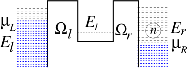
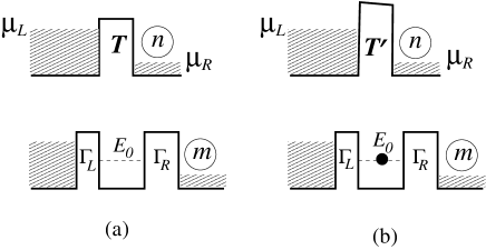
Let us consider a mesoscopic “device” consisting of a quantum well (dot), coupled to two separate electron reservoirs. The density of states in the reservoirs is very high (continuum). The dot, however, contains only isolated levels. We first demonstrate how to achieve the reduction of many-body Schroedinger equation to the rate equation in the simplest example, Fig. 1, with only one level, , inside the dot. We also ignore the Coulomb electron-electron interaction inside the well and the spin degrees of freedom. Hence, only one electron may occupy the well.
With the stand simplifications, the tunneling Hamiltonian of the entire system in the occupation number representation is
| (1) |
.
where and are the creation operators for the electron in the dot and in the left (right) reservoirs. The subscripts and enumerate correspondingly the levels in the left (emitter) and right (collector) reservoirs. The tunneling couplings of the dots to the leads, , are weakly dependent of energy (wide-band limit) and can be chosen to be real in the absence of magnetic field.
For simplicity, we restrict ourselves to the zero temperature in the reservoirs. All the levels in the emitter and the collector are initially filled with electrons up to the Fermi energy and , respectively. This situation will be treated as the “vacuum” state .
This vacuum state is unstable; the Hamiltonian Eq. (1) requires it to decay exponentially to a continuum state having the form with an electron in the level and a hole in the emitter continuum. These continuum states are also unstable and decay to states having a particle in the collector continuum as well as a hole in the emitter continuum, and no electron in the level . The latter, in turn, are decaying into the states and so on. The evolution of the whole system is described by the many-particle wave function, which is represented as
| (2) |
where are the time-dependent probability amplitudes to find the system in the corresponding states described above with the initial condition , and all the other ’s being zeros. Substituting Eq. (2) into in the Schrödinger equation , results in an infinite set of coupled linear differential equations for the amplitudes . Applying the Laplace transform
| (3) |
and taking account of the initial conditions, we transform the linear differential equations for into an infinite set of algebraic equations for the amplitudes ,
| (4a) | |||
| (4b) | |||
| (4c) | |||
| (4d) | |||
Note that in the Laplace transform , where plays a role of energy in the scattering theory.
Equations (4) can be substantially simplified. Let us replace the amplitude in the term of each of the equations by its expression obtained from the subsequent equation. For example, substitute from Eq. (4b) into Eq. (4a). We obtain
| (5) |
Since the states in the reservoirs are very dense (continuum), one can replace the sums over and by integrals, for instance , where is the density of states in the emitter. We assume that it is independent of the (wide band limit), and the same for the density of state of the collector, . Also the tunneling couplings are considered as the energy independent, . Then the first sum in Eq. (5) becomes an integral
| (6) |
where is a cut-off and is a partial width of the level due to its coupling to the emitter. (The corresponding partial width due to tunneling to the collector is ).
Now we consider the case of , corresponding to the energy level is deeply inside the bias, , (large bias limit). Then the last term of Eq. (6) vanishes in the limit of as (or ). We then obtain
| (7) |
Consider now the second sum in Eq. (5).
| (8) |
In contrast with the first term of Eq. (5), the amplitude is not factorized out the integral (8). We refer to this type of terms as “cross-terms”. Fortunately, all “cross-terms” vanish in the limit of large bias. This greatly simplifies the problem and is very crucial for a transformation of the Schrödinger to the Master equations. The reason is that the poles of the integrand in the -variable in the “cross-terms” are on the same side of the integration contour. One can find it by using a perturbation series the amplitudes in powers of . For instance, from iterations of Eqs. (4) one finds
| (9) |
The higher order powers of have the same structure. Since in the Laplace transform, all poles of the amplitude in the -variable are below the real axis. In this case, substituting Eq. (9) into Eq. (8) we find in the limit ,
| (10) |
Thus, in the large bias limit.
Applying analogous considerations to the other equations of the system (4), we finally arrive at the following set of equations:
| (11a) | |||
| (11b) | |||
| (11c) | |||
| (11d) | |||
Now we introduce the (reduced) density matrix of the “device”. The Fock space of the quantum well consists of only two possible states, namely: – the level is empty, and – the level is occupied. In this basis, the diagonal elements of the density matrix of the “device”, and , give the probabilities of the resonant level being empty or occupied, respectively. In our notation, these probabilities are represented as follows:
| (12a) | ||||
| (12b) | ||||
where the index in denotes the number of electrons in the collector, Fig. 1. The current flowing through the system is , where is the number of electrons accumulated in the collector, i.e.
| (13) |
In the following we adopt the units where the electron charge is unity.
The density submatrix elements are directly related to the amplitudes through the inverse Laplace transform,
| (14) |
By means of this equation one can transform Eqs. (11)) for the amplitudes into differential equations directly to the density matrix , where denote the state of the SET with an unoccupied or occupied dot and denotes the number of electrons which have arrived at the collector by time , Fig. 1. In fact, as follows from our derivation, the diagonal density-matrix elements, and , form a closed system in the case of resonant tunneling through one level. The off-diagonal elements, , appear in the equation of motion whenever more than one discrete level of the system carry the transport (see in following). Therefore we concentrate below on the diagonal density-matrix elements only, and . Applying the inverse Laplace transform on finds
| (15a) | |||||
| (15b) | |||||
Consider, for instance, the term . Multiplying Eq. (11b) by and then subtracting the complex conjugated equation with the interchange we obtain
| (16) |
Using Eq. (15b) one easily finds that the first integral in Eq. (16) equals to . Next, substituting
| (17) |
from Eq. (11b) into the second term of Eq. (16), and replacing a sum by an integral, one can perform the -integration in the large bias limit, , . Then using again Eq. (15b) one reduces the second term of Eq. (16) to . Finally, Eq. (16) reads .
The same algebra can be applied for all other amplitudes . For instance, by using Eq. (15a) one easily finds that Eq. (11c) is converted to the following rate equation . With respect to the states involving more than one electron (hole) in the reservoirs (the amplitudes like and so on), the corresponding equations contain the Pauli exchange terms. By converting these equations into those for the density matrix using our procedure, one finds the “cross terms”, like , generated by Eq. (11d). Yet, these terms vanish after an integration over in the large bias limit, as the second term in Eq. (5). The rest of the algebra remains the same, so one obtains . Finally we arrive to the following infinite system of the chain equations for the diagonal elements, and , of the density matrix,
| (18a) | |||
| (18b) | |||
| (18c) | |||
| (18d) | |||
Summing up these equations, one easily obtains differential equations for the total probabilities and :
| (19a) | ||||
| (19b) | ||||
which should be supplemented with the initial conditions
| (20) |
Using Eqs. (13), (18) we obtain the total current
| (21) |
Thus the current is directly proportional to the charge density in the well. Solving Eqs. (19) and substituting into Eq. (21), we obtain (for ) the standard formula for the dc resonant current,
| (22) |
Notice that whereas the time-behavior of the current depends on the initial condition, the stationary current , Eq. (22), does not.
Equations (19), derived from the many-body Schrödinger equation, coincide with the classical rate equations in the sequential picture for the resonant tunneling. However, as shows our derivation these equations can be valid only when the resonance energy is inside the bias, and (large bias limit). If the resonance is near the Fermi energy of a reservoir, the time-dependent Scrödinger equation cannot be reduced to the rate equations (19).
III Coulomb blockade
Now we extend the approach of Sect. II to include the effects of Coulomb interaction. Consider again the quantum well in Fig. 1, taking into account the spin degrees of freedom (). In this case the tunneling Hamiltonian (1) becomes
| (23) |
where , and is the Coulomb repulsion energy.
Writing down the many-body wave function, , in the occupation number representation, just as in Eq. (2), and then substituting it into the Schrödinger equation , we find a system of coupled equations for the amplitudes
| (24a) | |||
| (24b) | |||
| (24c) | |||
| (24d) | |||
In order to shorten notations we eliminated the index (1) of the level in the amplitudes , so that denotes the probability amplitude to find one electron inside the well with spin up (down), and the amplitude is the probability amplitude to find two electrons inside the well.
Equations (24) can be simplified by using the same procedure as described in the previous section. For instance, by substituting from Eq. (24c) and from Eq. (24d) into Eq. (24b), and neglecting the “cross terms” on the grounds of the same arguments as in the analysis of Eq. (5)), we obtain
| (25) |
where . Since , the singular parts of the integrals in (25) are respectively and , where
| (26) |
Here is the spin up or spin down density of states in the emitter (collector), . As in the previous section, we assume the resonance level being deeply inside the bias, . If, in addition, , the theta-function in the singular parts of the integrals in (25) can be replaced by one. In the opposite case, , the corresponding singular part is zero.
Proceeding this way with the other equations of the system (24), we finally obtain
| (27a) | |||
| (27b) | |||
| (27c) | |||
| (27d) | |||
Equations (27) can be transformed into equations for the density matrix of the “device” by using the method of the previous section. Since the algebra remains essentially the same, we give only the final equations for the diagonal density matrix elements , , and . These are the probabilities to find: a) no electrons inside the well; b) one electron with spin up (down) inside the well, and c) two electrons inside the well, respectively. The index denotes the number of electrons accumulated in the collector. We obtain
| (28a) | ||||
| (28b) | ||||
| (28c) | ||||
| (28d) | ||||
These rate equations look as a generalization of the rate equations (18), if one allows the well to be occupied by two electrons. The Coulomb repulsion leads merely to a modification of the corresponding rates , due to increase of the two electron energy.
Summing up the partial probabilities we obtain for the total probabilities, , the following equations:
| (29a) | |||
| (29b) | |||
| (29c) | |||
| (29d) | |||
It follows from Eq. (29) that . Respectively one finds for the current
| (30) |
Equations (29), (30) can be solved most easily for dc current, . In this case , and Eqs. (29) turn into the system of linear algebraic equations. Finally we obtain
| (31) |
so that dc current does not depend on the initial conditions.
If , one finds from Eq. (25) that , so that the state with two electrons inside the well is not available. In this case one obtains from Eq. (31) for the dc current
| (32) |
It is interesting to note that this result is different from Eq. (22), although in both cases only one electron can occupy the well. However, if the Coulomb repulsion effect is small, i.e. , Eq. (31) does produce the same result as Eq. (22), provided the density of states is doubled due to the spin degrees of freedom.
One can also consider the case when the Fermi level in the right reservoir lies above the resonance level , but below , so that , Eq. (25). Then the resonant transitions of electrons from the left to the right reservoirs can go only through the state with two electrons inside the well. Using Eq. (31) one finds for the dc current
| (33) |
which coincides with the result found by Glazmann and Matveevglaz .
IV Double-well structure
IV.1 Non-interacting electrons.
Now we turn to the coherent case of resonant tunneling. Let us consider the coupled-well structure, shown in Fig. 2. We assume that both levels are inside the bias, i.e. . In order to make our derivation as clear as possible, we begin with the case of no spin degrees of freedom and no Coulomb interaction.
.
The tunneling Hamiltonian for this system is
| (34) |
where , are creation and annihilation operators for an electron in the first or the second well, respectively. All the other notations are taken from Sect. II. The many-body wave function describing this system can be written in the occupation number representation as
| (35) |
Substituting Eq. (35) into the Shrödinger equation with the Hamiltonian (34) and performing the Laplace transform, we obtain an infinite set of the coupled equations for the amplitudes :
| (36a) | |||
| (36b) | |||
| (36c) | |||
| (36d) | |||
Using exactly the same procedure as in the previous sections, Eqs. (5)-(10), we transform Eqs. (36) into the following set of equations:
| (37a) | |||
| (37b) | |||
| (37c) | |||
| (37d) | |||
The amplitudes determine the density submatrix of the system, , in the corresponding Fock space: – the levels are empty, – the level is occupied, – the level is occupied, – the both level are occupied; the index denotes the number of electrons in the collector. The matrix elements of the density matrix of the “device” can be written as
| (38a) | |||
| (38b) | |||
| (38c) | |||
| (38d) | |||
| (38e) | |||
Now we transform Eqs. (37) into differential equations for . Consider for instance the term , Eq. (38b), where the amplitudes are determined by Eq. (37b). Multiplying Eq. (37b) by and subtracting the complex conjugate equation with , we find
| (39) |
After applying the inverse Laplace transform, Eqs. (14),(15) the first term in this equation becomes . Next, substituting
| (40) |
from Eq. (37b) into the second term of Eq. (39), and replacing the sum by an integral over , we reduce this term to . After the inverse Laplace transform it becomes . Notice that in the large bias limit, the “cross term”, , does not contribute to the integral over , since the poles of the integrand in the -variable lie on one side of the integration contour (cf. with Eq. (10)). The third term of Eq. (39) turns to be , after the inverse Laplace transform. Finally we obtain a differential equation for the density submatrix element ,
| (41) |
In contrast to the rate equations of the previous sections, the diagonal matrix element is coupled with the off-diagonal density matrix element .
The corresponding differential equation for can be easily obtained by multiplying Eq. (37b) by with subsequent subtracting the complex conjugated Eq. (37c), multiplied by . Then by integrating over we obtain
| (42) |
Eventually we arrive to the following set of equations for
| (43a) | ||||
| (43b) | ||||
| (43c) | ||||
| (43d) | ||||
| (43e) | ||||
Using Eqs. (43) we can find the charge accumulated in the collector, , and subsequently, the total current, , as given by
| (44) |
As in the previous examples, the current is proportional to the total probability of finding an electron in the well adjacent to the right reservoir. The off-diagonal elements of the density matrix do not appear in Eq. (44).
Summing up over in Eqs. (43), we obtain the system of differential equations for the density matrix elements of the device
| (45a) | |||
| (45b) | |||
| (45c) | |||
| (45d) | |||
| (45e) | |||
Eqs. (45)) resemble the optical Bloch equationsbloch . Note that the coupling with the reservoirs produces purely negative contribution into the non-diagonal matrix element’s dynamic equation, Eq. (45e), thus causing damping of this matrix element.
IV.2 Coulomb blockade.
The extension of the rate equations (45) for the case of spin and Coulomb interaction is done exactly in the same way as in Sec. III. Here also the rate equations for the device density matrix are obtained only for being inside or outside the bias, but not close to the bias edges ( or ). Eventually we arrive to the rate equations of type Eqs. (45), but with the number of the available states of the device changed due to additional (spin) degrees of freedom and Coulomb blockade restrictions. The Coulomb repulsion manifests itself also in a modification of the transition amplitude and the rates ’s, Eq. (26).
In the case of large Coulomb repulsion, some of electron states of the device are outside the bias (the Coulomb blockade). As a result, the number of the equations is reduced. Consider, for instance, the situation where the Coulomb interaction of two electrons in the same well so large that , but the Coulomb repulsion of two electrons in different wells, , is much smaller, so that . Then the state of two electrons in the same well is not available, but two electrons can occupy different wells. In this case the rate equations for the corresponding density matrix elements of the device are
| (47a) | |||
| (47b) | |||
| (47c) | |||
| (47d) | |||
| (47e) | |||
where . Here for the shortness we wrote only the equations for the “spin up” component of the density matrix. The same equations are obtained for the “spin down” components of the density matrix. The total current is
| (48) |
It is quite clear that the “spin up” and “spin down” components of the density matrix are equal, i.e. , the same holding for , components. Therefore Eqs. (47), (48) can be rewritten as
| (49a) | ||||
| (49b) | ||||
| (49c) | ||||
| (49d) | ||||
| (49e) | ||||
and
| (50) |
Using we obtain for the dc current
| (51) |
where . Notice that the current (51) differs from that given by Eq. (46) even for and , despite the fact that in the both cases only one electron can occupy each of the wells.
It is interesting to compare our result with that of Stoof and Nazarovnaz1 for the case of strong Coulomb repulsion between two electrons in different wells (), where only one electron can be found inside the system. It corresponds to . In this case the dc current given by Eq. (51) is
| (52) |
This result is slightly different from that obtained by Stoof and Nazarov (by the factor two in front of ). The difference stems from the account of spin components in the rate equations, which has not been done innaz1 .
V Inelastic processes
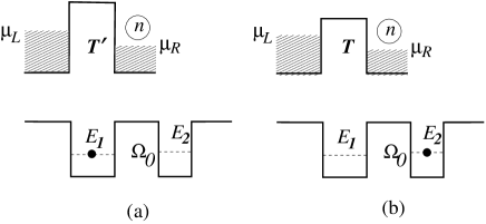
As an example of a system with coherent tunneling accompanied by inelastic scattering, let us consider the coupled-dot structure shown in Fig. 3. In this system a resonant current flows due to inelastic transition from the upper to the lower level in the left well. For simplicity, we restrict ourselves to non-interacting spin-less electrons. The Coulomb interaction and the spin effects can be accounted for precisely in the same way as we did in the previous sections.
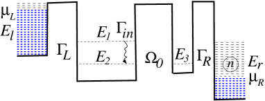
The tunneling Hamiltonian of the system has the following structure
| (53) |
Here the subscript enumerates the states in the phonon bath and is the corresponding coupling. The many particle time-dependent wave function of the system is
| (54) |
Repeating the procedure of the previous sections we find the following set of equations for the Laplace transformed amplitudes, :
| (55a) | |||
| (55b) | |||
| (55c) | |||
| (55d) | |||
| (55e) | |||
| (55f) | |||
where is the partial width of the level due to phonon emission and is the density of phonon states.
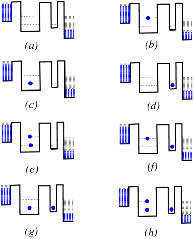
The density matrix elements of the device is , where , are related to the amplitudes via Eqs. (14), (15) All possible electron states of the device are shown in Fig. 4.
Using the previous section procedure for diagonal matrix elements we obtain master equations analogous to Eq. (45), in which transitions between isolated levels and take place through the coupling with non-diagonal matrix elements. These equations have the appearance of the optical Bloch equationbloch . However, the master equation for the non-diagonal matrix element (coherences) contains an additional term. Therefore, we present the derivation of the master equations for “coherences” and in some detail.
Consider for example the non-diagonal density submatrix elements and . The differential equation for can be obtained by multiplying Eq. (55c) by with subsequent subtraction of the complex conjugated Eq. (55d), multiplied by . Then using Eq. (14), (15) we obtain
| (56) |
Similarly, multiplying Eq. (55e) by and Eq. (55f) by , we find the differential equation for
| (57) |
where
| (58) |
Substituting the amplitudes from Eq. (55e) and from Eq. (55f) into Eq. (58), and replacing the sum over by the corresponding integral, we find . It implies that the non-diagonal density matrix given by Eq. (57), is coupled with via a single electron transition from the emitter to the left well. Obviously, such a term does not appear in the Bloch equations, which deal with two-level systems.
Summing up over in the rate equations for the density submatrix we obtain the set of rate equations for the density matrix of the device
| (59a) | ||||
| (59b) | ||||
| (59c) | ||||
| (59d) | ||||
| (59e) | ||||
| (59f) | ||||
| (59g) | ||||
| (59h) | ||||
| (59i) | ||||
| (59j) | ||||
and the resonant current flowing through this system is .
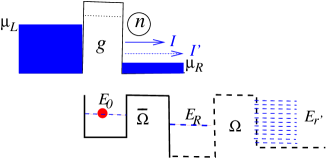
VI Master equations for two wells separated by continuum
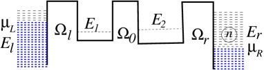
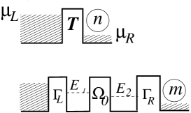
Let us consider quantum transport through two quantum wells (quantum dots). separated by a ballistic channel, as shown schematically in Fig. 5.

The dots contain only isolated levels, whereas the density of states in the ballistic channel and in the emitter and the detector is very high (continuum). This system can be described by the tunneling Hamiltonian
| (60) |
where . The subscripts , and enumerate correspondingly the levels in the left reservoir, in the (middle) ballistic channel and in the right reservoir. The spin degrees of freedom were omitted.
In order to simplify the derivation we assumed that the intradot charging energy is large, . Thus only one electron can occupy each of the dots. However, the interdot charging energy is much smaller, so it does not prevent simultaneous occupation of the two dots. The same is assumed for the Coulomb repulsion between electrons inside the dots and the ballistic channel. Although we did not include this interaction in the Hamiltonian (60), it can be treated in the same way as the interdot interaction . As in the previous case we restrict ourselves to the zero temperature case, even though the results are valid for a finite temperature, as would be clear from the derivation.
Let us assume that all the levels in the emitter, in the ballistic channel and in the collector are initially filled up to the Fermi energies , and respectively. We call it as the “vacuum” state, . (In the following we consider the case of large bias, so that ). The many-body wave function describing this system can be written in the occupation number representation as
| (61) |
where are the time-dependent probability amplitudes to find the system in the corresponding states described above. These amplitudes are obtained from the Shrödinger equation , supplemented with the initial condition (, and all the other ’s being zeros). Using the amplitudes we can find the density-matrix of the quantum dots, , by tracing out the continuum states of the reservoirs and the ballistic channel. Here the subscript indices in denote four states of the dots: , where – the levels are empty, – the level is occupied, – the level is occupied, – the both level are occupied, and the superscript indices denote the number of electrons accumulated in the ballistic channel and in the collector respectively at time , Fig. 6,

One finds
| (62a) | |||
| (62b) | |||
| (62c) | |||
The rate of electrons arriving to the collector determines the electron current in the system. Therefore the current operator is , where is the operator for the total number of electrons accumulated in the right reservoir. Using Eqs. (60), (61), (62) we find that the current flowing through the system is
| (63) |
As expected, is the time derivative of the total charge accumulated in the collector. Thus the current flowing through this system is expressed in terms of the diagonal elements of the density-matrix . In order to find the differential equations for we need to sum over the states of the reservoirs and the ballistic channel, Eqs. (62).
As in previous sections, we use the Laplace transform for the Shrödinger equation, . Then the amplitudes in the wave function (61) are replaced by their Laplace transform, , Eq. (3). Substituting Eq. (61) into the Shrödinger equation we obtain an infinite set of coupled equations for the amplitudes :
| (64a) | |||
| (64b) | |||
| (64c) | |||
| (64d) | |||
| (64e) | |||
Note that due to the Pauli principle an electron can return back only into unoccupied states of the emitter. As a result, the summation over the emitter states does not appear in the corresponding terms of Eqs. (64) (in the second term of Eq. (64b), in the second and the third terms of Eq. (64c), and so on).
Now we replace the amplitude in the term of each of the equations (64) by its expression obtained from the subsequent equation. For example, substitute from Eq. (64b) into Eq. (64a). We obtain
| (65) |
where and . In the wide-band limit, this expression is treated exactly in the same way as Eq. (5). Namely, we replace the sums over and by integrals, like , where is the density of states in the emitter. Then the first sum in Eq. (65) becomes an integral which can be split into a sum of the singular and principal value parts. The singular part yields , where is the level partial width due to coupling to the emitter. In the large bias limit, , the integration over -variables can be extended to . As a result, the theta-function can be replaced by one, whereas the principal p[art vanishes (see Eqs. (6), (7)). The second sum (integral) in Eq. (65) vanishes as well, since the poles of the integrand in the -variable are on one side of the integration contour (c.f. with Eqs. (8)-(10)). In general, any terms of the type , whenever the integration over the -variable can be extended to . We shall imply this property in all subsequent derivations. Notice that these results are valid also for non-zero temperature, providing that .
Now we apply analogous considerations to the other equations of the system (64). However, in order to be able to carry it, we need to impose some restriction on a geometry of the ballistic channel, separated two wells, Fig. 5. This already appears by treating the last term of Eq. (64b), which we denote as . Substituting the amplitude , obtained from Eq. (64c) into this term and replacing the sum by integral, we find
| (66) |
In the large band limit, the spectral functions and are weakly dependent of energy . However the relative sign of and can strongly oscillate with .
Indeed the tunneling couplings are given by the overlap of localized wave functions, belonging to the dot states, , with an extended wave function, belonging to the reservoir state . Since the latter belongs to continuum, the corresponding wave function would oscillate inside the middle reservoir. Then the sign[] will oscillate as well with a frequency , where is a length of the reservoir. This creates a problem of how to make the product of the both couplings energy independent. in order to perform the -integration in the same way, as we did in Eqs. (5), (65).
The problem can be avoided by coupling two quantum dots to a common reservoir (ballistic channel) at close points, similar to the setup in Refs. [wolf, ; xq1, ; xq2, ] and shown in Fig. 7.

This would make the product independent of the energy in the wide-band limit. Thus , so that the integration in Eq. (66) and in similar terms can be performed as in Eqs. (6), (7), finally arriving at the following set of equations:
| (67a) | |||
| (67b) | |||
| (67c) | |||
| (67d) | |||
| (67e) | |||
where and are the partial widths of the levels and , respectively due to coupling to the ballistic channel with the density of states , and are partial widths due to coupling to the emitter and collector. The Coulomb interdot repulsion just shifts the energy of the corresponding dot, as in Eq. (67e). In the case of Coulomb blockade, , the corresponding amplitude vanishes (c.f. with Eqs. (27)).
The density matrix elements, Eqs. (62), are directly related to the amplitudes through the inverse Laplace transform, Eqs. (14), (15). Using this equation one can transform Eqs. (67) for the amplitudes into differential equations for the probabilities . Consider, for instance, the term , Eq. (62b). Multiplying Eq. (67b) by and then subtracting the complex conjugated equation with the interchange we obtain
| (68) |
Substituting
| (69) |
into Eq. (68) we can carry out the -integrations thus obtaining
| (70) |
Applying the same procedure to each of equations (67c), we obtain the following Bloch-type rate equations for the matrix elements of the density-submatrix :
| (71a) | |||
| (71b) | |||
| (71c) | |||
| (71d) | |||
| (71e) | |||
Equations (71) have clear physical interpretation. Consider for instance Eq. (71a) for the probability rate of finding the system in the state with electrons in the ballistic channel and electrons in the right reservoir (Fig. 6a). This state decays with the rate into the state (Fig. 6b) whenever an electron enters the first dot from the left reservoir. This process is described by the first term in Eq. (71a). On the other hand, the states and (Figs. 6b,c) with electrons in the ballistic channel decay into the state with electrons in the ballistic channel. It takes place due to one-electron tunneling from the quantum dots into the ballistic channel with the rates and respectively. This process is described by the second and the third terms in Eq. (71a). Also the state (Fig. 6c) with electrons in the right reservoir can decay into the state due to tunneling to the right reservoir with the rate (the fourth term in Eq. (71a)). The last term in this equation describes the decay of coherent superposition of the states and into the state . It takes place due to single electron tunneling from the first and the second dots into the same state of the ballistic channel with the amplitudes and , respectively. Obviously, this process has no classical analogy, since classical particle cannot simultaneously occupy two dots.
Equations (71b), (71c) and (71d) describe the probability rate of finding the system in the states where one of the dots or both dots are occupied. In the first case an electron can jump into unoccupied dot via continuum states of the ballistic channel. As a result, the states and can decay into linear superposition of the states and . This process is described by the last terms in Eqs. (71b), (71c). Obviously, if the both dots are occupied, such a process cannot take a place. Therefore is not coupled with the nondiagonal density-matrix elements, Eq. (71d). The last equation, (71e) describes the time-dependence of the nondiagonal density matrix element. It has the same interpretation as all previous equations.
Equations (71) for the reduced density matrix were derived starting from the wave function , Eq. (61), where all the levels of the reservoirs are occupied up to the corresponding Fermi energies. In fact, at finite temperature, the system is not initially in a pure state, but in incoherent superposition of different pure state, weighted by the corresponding Fermi function. The final answer therefore should be averaged over this distribution. In our case, however, it is not relevant, since we consider the large bias limit. Then energy levels of the dots are far away from the Fermi-levels, such that (). Thus, the reservoir levels that carry the current () are deeply inside the Fermi sea, so they can be considered as fully occupied. Hence, one would arrive to the same Eqs. (71).
Using Eqs. (71) one finds for the total current, Eq. (63)
| (72) |
where are the total “probabilities”. We can easily understand this result by taken into account that is the total probability for occupation of the second dot and is the rate of electron transitions from this dot to the (adjacent) right reservoir.
In order to find differential equations for we sum over in Eqs. (71). Then we obtain the following Bloch-type equations, which describe the time-dependence of the density-matrix for separated dots xq3
| (73a) | |||
| (73b) | |||
| (73c) | |||
| (73d) | |||
| (73e) | |||
where . Note that , since the amplitudes , can be of the opposite signs due to different parity of the dots localized states parity .
The stationary (dc) current Eq. (72) can be easily obtained from Eqs. (73) by taken into account that for . As a result, Eqs. (73) turn into a system of linear algebraic equations, supplemented by a probability conservation condition . Consider, for example, the case of the same of . Solving Eqs. (72), (73) one finds for dc current xq3
| (74) |
where .
Similar to the coupled-dot case, Eq. (46), dc current in separated dots displays the Lorentzian shape resonance as a function of and the same peculiar dependence on the coupling with the collector. Indeed, contrary to expectations, the current vanishes when . The latter manifests the quantum-coherence effects in double-dot and separated dot systems xq3 .
VII General case
The (number resolved) rate equations (71), describing electron transport in separated dots, can be extended to any multi-dot system. By applying the same technique of integrating out the reservoir states discussed above, we arrive to the rate equations for the density-matrix of the multi-dot system, where denote the number of electrons, arriving to corresponding reservoirs. Tracing over , these equations can be written in a general form as xq3 ; gm
| (75) |
where denote all discrete states of the multi-dot system in the occupation number representation, and denotes one-electron hopping amplitude that generates -transition. We distinguish between the amplitudes and of one-electron hopping among isolated states and among isolated and continuum states, respectively. The latter transitions are of the second order in the hopping amplitude . These transition are produced by two consecutive hoppings of an electron across continuum states with the density of states . The first of these terms arises from “loss” processes and the second from “gain” processes (borrowing the terminology of the classical Boltzmann equation). is the Pauli factor: in transitions involving two electrons, +1 otherwise.
Applying these rules, it is rather easy to verify that Eqs. (75) coincide with Eqs. (73) for , which are the states of the separated dot system, shown in Fig. 6. In addition, Eqs. (75) have the same form for the number-resolved density matrix, . One only needs to take into account that the number of electron indicated in each of the term in the rhs of this equation is the same as in the lhs, if the electron returns to the same reservoir, or it is less by one, if a new electron arrives to the another reservoir, (see Eqs. (28),(43),(71)).
It is easy to realize that Eq. (75) has precisely a form of the Lindblad equation lind , which for the -dimensional system reads
| (76) |
where is the system Hamiltonian, is the Lindblad operator and . However, one should emphasize, that the necessary conditions for derivation of Eq. (75) are the Markovian environment and reservoirs (energy independent spectral density function) and large bias limit.
VIII Description of measurement by rate equations
VIII.1 Ballistic point-contact detector
Consider the measurement of electron occupation of a semiconductor quantum dot by means of a separate measuring circuit in close proximitypep ; buks3 . A ballistic one-dimensional point-contact is used as a “detector” that resistance is very sensitive to the electrostatic field generated by an electron occupying the measured quantum dot. Such a set up is shown schematically in Fig. 8, where the detector is represented by a barrier, connected with two reservoirs at the chemical potentials and respectively. The transmission probability of the barrier varies from to , depending on whether or not the quantum dot is occupied by an electron, Fig. 8(a,b).
Initially all the levels in the reservoirs are filled up to the corresponding Fermi energies and the quantum dot is empty. (For simplicity we consider the reservoirs at zero temperature). The time-evolution of the entire system can be described by the following master (rate) equations. which we derive in next subsections
| (77a) | ||||
| (77b) | ||||
where and are probabilities of finding the entire system in the states and corresponding to empty or occupied dot Fig. 8(a,b), and and are the number of electrons penetrated to the right reservoirs of the measured system and the detector, respectively. are the transition rates for an electron tunneling from the left reservoir to the dot and from the dot to the right reservoir respectively, and is the rate of electron hopping from the right to the left reservoir through the point-contact (the Landauer formula).
The accumulated charge in the right reservoirs of the detector () and of the measured system () is given by
| (78a) | ||||
| (78b) | ||||
The currents flowing in the detector and in the measured system are and . Using Eqs. (77) and (78) we obtain
| (79a) | ||||
| (79b) | ||||
where and are the total probabilities of finding the dot empty or occupied. Obviously , where . Performing the summation over in Eqs. (77) we obtain the following rate equation for the quantum dot occupation probability
| (80) |
If the point-contact and the quantum dot are decoupled, the detector current is . Hence, the occupation of the quantum dot can be measured through the variation of the detector current . One readily obtains from Eq. (79b) that
| (81) |
where is the voltage bias, and . Thus, the point contact is indeed the measurement device. In fact, Eq. (81) is a self-evident one. Indeed, the variation of the point-contact current is and is the probability for such a variation.
VIII.2 Derivation of the rate equations for a point-contact detector
We present here the microscopic derivation of the rate equations describing electron transport through the point contact. The latter is considered as a barrier, separated two reservoirs (the emitter and the collector), Fig. 8. The system is described by the tunneling Hamiltonian
| (82) |
where and are the creation (annihilation) operators in the left and the right reservoirs, respectively, and is the hopping amplitude between the states and in the right and the left reservoirs. (We choose the the gauge where is real).
Consider all the levels in the emitter and the collector are initially filled up to the Fermi energies and respectively, Fig. 8. We call it as the “vacuum” state, . The Hamiltonian Eq. (82) requires the vacuum state to decay to continuum states having the form: with an electron in the collector continuum and a hole in the emitter continuum; with two electrons in the collector continuum and two holes in the emitter continuum, and so on. The many-body wave function describing this system can be written in the occupation number representation as
| (83) |
where are the time-dependent probability amplitudes to find the system in the corresponding states with the initial condition , and all the other ’s being zeros. Substituting Eq. (83) into the Shrödinger equation and performing the Laplace transform , Eq. (3), we obtain an infinite set of the coupled equations for the amplitudes :
| (84a) | |||
| (84b) | |||
| (84c) | |||
Eqs. (84) can be substantially simplified by replacing the amplitude in the term of each of the equations by its expression obtained from the subsequent equation (c.f. Eqs. (5), (65)). For example, substituting from Eq. (84b) into Eq. (84a), one obtains
| (85) |
where we assumed that the hopping amplitudes are weakly dependent functions on the energies (wide-band limit). Since the states in the reservoirs are very dense (continuum), one can replace the sums over and by integrals, for instance , where are the density of states in the emitter and collector. Then the first sum in Eq. (85) becomes an integral which can be split into a sum of the singular and principal value parts. The singular part yields , whereas the principal value part can be neglected in the large bias limit, Eqs. (6), (7). The second sum in Eq. (85) can be neglected either. Indeed, by replacing and the sums by the integrals we find that the integrand has the poles on the same sides of the integration contours. It implies that the corresponding integral vanishes (c.f. with Eqs. (8), (10)).
Applying analogous considerations to the other equations of the system (84), we finally arrive to the following set of equations:
| (86a) | |||
| (86b) | |||
| (86c) | |||
where .
The charge accumulated in the collector at time is
| (87) |
where
| (88) |
are the probabilities to find electrons in the collector. These probabilities are directly related to the amplitudes through the inverse Laplace transform,
| (89) |
Using Eq. (89) one can transform Eqs. (86) into the rate equations for . We find
| (90a) | |||
| (90b) | |||
| (90c) | |||
VIII.3 Transmission coefficient of the point-contact.
Now we relate the coupling of the tunneling Hamiltonian (82) to the transmission coefficient of the point-contact. The latter determines probability of penetration of a single electron from the left to the right lead at . For this reason we consider single-electron motion from the emitter to collector.
A single-electron wave-function in the basis of the reservoir states, (, ) can be written as
| (93) |
where the index denotes the electron initial state, occupying a level in the left reservoir. Substituting (93) in the Schrödinger equations, , we find
| (94) |
In order to solve these equations we apply the Laplace transform, , Eq. (3). Then Eqs. (94) become
| (95) |
Let us introduce and . Then Eqs. (95) can be rewritten as
| (96) |
where
| (97) |
In the continuous limit one obtains (c.f. Eqs. (6), (7))
| (98) |
where the cutoff . Then solving Eqs. (96) one easily finds
| (99) |
and finally
| (100) |
The probability of finding the electron in the right lead at time is given by , where
| (101) |
Then using Eq. (100) we obtain in the continuous limit
| (102) |
where .
Let us evaluate the electric current in the left reservoir, . One finds
| (103) |
We consider the initial electron state as given by incoherent superposition of different states with a distribution . In the case we obtain
| (104) |
This in fact represents the Landauer formula
| (105) |
where
| (106) |
represents a relation between transmission coefficient and coupling in the tunneling Hamiltonian.
IX Detection of electron oscillations in coupled-dots
A well-known manifestation of quantum coherence is the oscillation of a particle in a double-well (double-dot) potential. The origin of these oscillations is the interference between the probability amplitudes of finding a particle in different wells. Hence, one can expect that the disclosure of a particle (electron) in one of wells would generate the “dephasing” that eventually destroys these oscillations.
Let us investigate the mechanism of this process by taking for detector a noninvasive point-contact. A possible set up is shown in Fig. 10.
We assume that the transmission probability of the point-contact is when an electron occupies the right well, and it is when an electron occupies the left well. Here since the right well is away from the point contact.
Now we apply the quantum-rate equations to the whole system. However, in the distinction with the previous case, the electron transitions in the measured system take place between the isolated states inside the dots. As a result the diagonal density-matrix elements are coupled with the off-diagonal elements, so that the corresponding rate equations are the Bloch-type equations Eqs. (43).
We first start with the case of the double-well detached from the point-contact detector. The Bloch equations describing the time evolution of the electron density-matrix have the following form
| (107a) | ||||
| (107b) | ||||
| (107c) | ||||
where and is the coupling between the left and the right wells. Here and are the probabilities of finding the electron in the left and the right well respectively, and are the off-diagonal density-matrix elements (“coherences”)bloch .
Solving these equations for the initial conditions and and we obtain
| (108) |
where . As expected the electron initially localized in the first well oscillates between the wells with the frequency . Notice that the amplitude of these oscillations is . Thus the electron remains localized in the first well if the level displacement is large, .
Now we consider the electron oscillations in the presence of the point contact detector, Fig. 10. The corresponding Bloch equations for the entire system have the following form, see Eq. (75) (detailed microscopic derivation of these equations is given below)
| (109a) | |||
| (109b) | |||
| (109c) | |||
Here the index denotes the number of electrons arriving to the collector at time , and is the transition rate of an electron hopping from the left to the right detector reservoirs, , Eqs. (86). Notice that the presence of the detector results in additional terms in the rate equations in comparison with Eqs. (107). These terms are generated by transitions of an electron from the left to the right detector reservoirs with the rates and respectively. The equation for the non-diagonal density-matrix elements , Eq. (109c), is different from the standard Bloch equations due to the last term, which describes transition between different coherences, and . This term appears in the Bloch equations for coherences whenever the same hopping () takes place in the both states of the off-diagonal density-matrix element ( and ), Eq. (75). The rate of such transitions is determined by a product of the corresponding amplitudes ( and ).
It follows from Eqs. (79), (109) that the variation of the point-contact current measures directly the charge in the first dot. Indeed, one obtains for the detector current
| (110) |
where . Therefore is given by Eq. (81), where .
In order to determine the influence of the detector on the double-well system we trace out the detector states in Eqs. (109) thus obtaining
| (111a) | ||||
| (111b) | ||||
| (111c) | ||||
where , and are two values of the Point-Contact current, corresponding to the occupied right or left dot in Fig. (10).
Equations (111) coincide with Eqs. (107), describing the electron oscillations without detector, except for the last term in Eq. (111c). The latter generates the exponential damping of the non-diagonal density-matrix element with the “dephasing” rate
| (112) |
It implies that for . We can check it by looking for the stationary solutions of Eqs. (111) in the limit . In this case and Eqs. (111) become linear algebraic equations, which can be easily solved. One finds that the electron density-matrix becomes the statistical mixture.
| (113) |
Notice that the damping of the nondiagonal density matrix elements is coming entirely from the possibility of disclosing the electron in one of the wells. Indeed, if the detector does not distinguish which of the wells is occupied, i.e. , then .
The Bloch equations (109), (111) display explicitly the mechanism of dephasing during a noninvasive measurement, i.e. that which does not distort the energy levels of the measured system. The dephasing appears in the reduced density matrix as the “dissipative” term in the nondiagonal density matrix elements only, as a result of tracing out the detector variables. All other terms related to the detector are canceled after tracing out the detector variables.
IX.1 Continuous measurement and Zeno effect
The most surprising phenomenon which displays Eq. (113) is that the transition to the statistical mixture takes place even for a large displacement of the energy levels, , irrespectively of the initial conditions. It means that an electron initially localized in one of the wells would be always delocalized at . It would happened even if the electron was initially localized at the lower level. (Of course it does not violate the energy conservation, since the double-well is not isolated). Such a behavior is not expectable because the amplitude of electron oscillations is very small for large level displacement, Eq. (108). Thus, the electron should stay localized in one of the wells. One could expect that the continuous observation of this electron by a detector could only increase its localization. It can be inferred from so called Zeno effectzeno . The latter tells us that repeated observation of the system slow down transitions between quantum states due to the collapse of the wave function into the observed state. Since in our case the change of the detector current, monitors in the left well, Eqs. (81), (110), it represents the continuous measurement of the charge in this well. Nevertheless the effects is just opposite – the continuous measurement delocalizes the system (so-called, anti-Zeno effect anzeno ).
However, our results for small are in an agreement with the Zeno effect, even so we have not explicitly implied the projection postulate. For instance, Fig. 11 a shows the time-dependence of the probability to find an electron in the left dot, as obtained from the solution of Eqs. (111) for the aligned levels (), and (dashed curve), (dot-dashed curve) and (solid curve). One finds that for small the rate of transition from the left to the right well decreases with the increase of .

The same slowing down of the transition rate for small enough we find for the disaligned levels () in Fig. 11 b. However, with increase of , the continuous measurement leads to the electron delocalization (the anti-Zeno effect anzeno ; eg2 ), whereas in the absence of detector an electron would stay localized in the left well (the dashed curve in Fig. 11 b)
IX.2 Derivation of Master equations, describing double-dot under continuous measurement.
Although the rate equations (109) is a particular case of general Master equations (75), it is desirable to present a microscopic derivation of Eqs. (109) by using our wave-function approach. We start with the many-body Schrödinger equation, for the entire system. Here is the total Hamiltonian, which can be written as . Here is the Hamiltonian for the point-contact detector, Eq. (82); is the Hamiltonian for the measured double-dot system,
| (114) |
and describes the interaction between the detector and the measured system. Since the presence of an electron in the left well results in an effective increase of the point-contact barrier (), we can represent the interaction term as
| (115) |
The many-body wave function for the entire system can be written as
| (116) |
where are the probability amplitudes to find the entire system in the states defined by the corresponding creation and annihilation operators. Notice that Eq. (116) has the same form as Eq. (83), where only the probability amplitudes acquire an additional index (’1’ or ’2’) that denotes the well, occupied by an electron. Proceeding in the same way as in Sec. VIII B, we arrive to an infinite set of the coupled equations for the amplitudes , which are the Laplace transform (3) of the amplitudes
| (117a) | |||
| (117b) | |||
| (117c) | |||
| (117d) | |||
The same algebra as that used before allows us to simplify these equations, which then become
| (118a) | |||
| (118b) | |||
| (118c) | |||
| (118d) | |||
where .
Using the inverse Laplace transform (89) we can transform Eqs. (118) into differential equations for the density-matrix elements (=1,2)
| (119) |
where denotes the number of electrons accumulated in the collector. Consider, for instance the off-diagonal density-matrix element . The corresponding differential equation for this term can by obtained by multiplying Eq. (118c) by and subtracting the complex conjugated Eq. (118d) multiplied by . We then obtain
| (120) |
One easily finds that the first term in this equation equals to and the third term equals to . In order to evaluate the second term in Eq. (120) we replace by the integrals and substitute
| (121) |
obtained from Eqs. (118c), (118d), into Eq. (120). Then integrating over we find that the second term in Eq. (120) becomes . Thus Eq. (120) can be rewritten as
| (122) |
which coincides Eq. (109c) for and , , . Applying the same procedure to each of the equations (118) we arrive to Eqs. (109) for density matrix elements .
IX.3 Measurement of resonant current through a double-dot.
Measurement of decoherence rate, , generated by a measurement device, is a very important issue in quantum computation. It can be done via direct monitoring of damping rate of the single-electron oscillations in coupled-dots, Figs. 10, 11. However, the same can be extracted from the steady-state current, flowing through the double-dot. It is shown schematically in Fig. 12, where the coupled-dot is connected to two reservoirs (emitter and collector). For the sake of simplicity we assume strong inner and inter-dot Coulomb repulsion, so only one electron can occupy this system. Then there are only three available states of the coupled-dot system: the dots are empty (), the first dot is occupied () and the second dot is occupied (). Using Eq, (75), we write the following rate equations for the density matrix describing the entire system (c.f. with Eqs. (77), (109))
| (123a) | |||
| (123b) | |||
| (123c) | |||
| (123d) | |||
where the indices and denote the number of electrons arrived at time to the upper and the lower collector reservoir, respectively. Here , are the rates of electron transitions from the left reservoir to the first dot and from the second dot to the right reservoir, and is the amplitude of hopping between two dots.
The currents in the double-dot system () and in the detector () are given by Eqs. (79):
| (124a) | |||
| (124b) | |||
where . It follows from Eq. (124b) that the variation of the detector current is given by Eq. (81), where .
Performing summation in Eqs. (123) over the number of electrons arrived to the collectors (), we obtain the following Bloch-type equations for the reduced density-matrix of the double-dot system:
| (125a) | |||
| (125b) | |||
| (125c) | |||
| (125d) | |||
where is the dephasing rate generated by the detector, Eq. (112). Solving these equations in the limit we find the following expression for the current , Eq. (124a), flowing through the double-dot system
| (126) |
By analyzing Eq. (126) one finds that the decoherence rate, , Eq. (112), generated by the measurement, would affect the resonant current, . As an example, we display it in Fig. 13 for three values of decoherence rate: , and . We find that for small the current decreases with , while for large the average distribution of an electron in the dots remains the same. However, for larger values of the current increases with . It reflects electron delocalization in a double-well system, Fig. 11 b, due to continuous monitoring of the charge in the left dot. Thus, by measure the resonant current for different values of or (and) , one can extract the desirable decoherence rate,

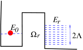
X Continuous measurement of decay to a non-Markovian reservoir
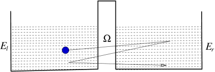
X.1 Tunneling to continuum.
Consider tunneling of a particle (electron) from a potential well (quantum dot) to a reservoir, Fig. 14. The system is described by the following Hamiltonian
| (127) |
Here is a localized state in the well and denotes extended states of the reservoir.
The tunneling of a particle to the reservoir is described by the Schrödiger equation,
| (128) |
where can be written as
| (129) |
Here is probability amplitude for finding the particle at the state inside the well and is the same for the state inside the reservoir. Substituting Eq. (129) into Eq. (128) and performing the Laplace transform, Eq. (3) we can rewrite Eq. (128) as
| (130a) | |||
| (130b) | |||
where the right-hand-side corresponds to the initial conditions.
Solving Eqs. (130) in the continuous limit, , where is the density of state, we find
| (131) |
with . In the case of Markovian reservoir (wide-band limit, ), the density of states and the coupling are independent of . Then integration over in Eq. (131) can be easily performed, thus obtaining
| (132) |
where . Note that for infinite reservoir, the density of states , where is the reservoir’s size, but , so the product (spectral density function) remains finite.
The amplitude is obtained from via the inverse Laplace transform,
| (133) |
As a result, probability of finding a particle inside the well (survival probability) . Thus in the wide-band limit, the particle initially localized inside the quantum well, decays exponentially to the reservoir.
Consider now a (non-Markovian) reservoir of a finite band-width, Fig. 14. It corresponds to a periodic one-dimensional chain of quantum wells, with the nearest-neighbor coupling , shown in Fig. 15 and describing by the following Hamiltonian
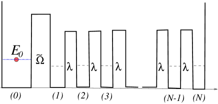
| (134) |
The state of the quantum well is coupled with the first site of the chain by coupling , so the total Hamiltonian is . By diagonalizing one arrives to Eq. (127) with
| (135a) | ||||
| (135b) | ||||
so that , and the corresponding spectral function is
| (136) |
where is the density of states and . Here the band-center . The Markovian case (wide-band limit) corresponds to . We assume that remains finite in this limit, which requires .
In our calculations we approximate the spectral function (136) by the Lorentzian
| (137) |
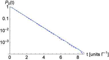
where is the Lorentzian center, and , providing the same curvature at the band-center that of Eq.(136). Such approximation allows us to treat the problem analytically without loosing its main physical features. For instance, Fig. 16 shows survival probability , obtained from Eqs. (130) and (135) for , and (dashed line) in comparison with the Lorentzian spectral function, Eq. (137), (solid line). One finds that both curves almost coincide. This confirms that the Lorentzian (137) is a very good approximation for finite band-width reservoirs, Eq.(136).
Substituting Eq. (137) in Eq. (131), we can evaluate the integral by closing the integration contour into lower complex -plane. As a result, Eq. (131) becomes
| (138) |
(In the following we choose .) Using the inverse Laplace transform, Eq. (133), we obtain
| (139) |
where and . In the limit we return to the Markovian case by reproducing the exponential decay, Eq. (133), whereas for finite , Eq. (139) reproduces two-exponential decay. The difference with Markovian case is mostly significant for small times . Indeed, the probability of decay to the Markovian reservoir, Eq. (133), reveals the irreversible dynamics, , whereas for the non-Markovian case, Eq. (139) the dynamics is reversible,
| (140) |
This makes a crucial importance for the quantum Zeno effect in continuous monitoring of decay to the non-Markovian reservoir. For a most effective treatment of this problem, we introduce a new basis for states of the non-Markovian reservoir.
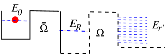
X.2 New basis of the reservoir’s states.
Consider Eq. (138) for the amplitude . Let us introduce the auxiliary amplitude (c.f. with Ref. [eg2, ])
| (141) |
where
| (142) |
Then Eqs. (138), (141) can be rewritten as
| (143a) | |||
| (143b) | |||
Let us demonstrate that Eqs. (143) describe the particle in a double-well, shown in Fig. 17, where the second well is a fictitious one, coupled with a fictitious Markovian reservoir, with the coupling and density of states , such that . This system is described by the Hamiltonian
| (144) |
Comparing (144) with the original Hamiltonian, Eqs. (127), we find that the reservoir’s (extended) states are split into the two components
| (145) |
where represent the extended states of the fictitious Markovian reservoir.
Now the particle wave function can be written in this new basis as
| (146) |
Substituting it in the Schrödinger equation we find
| (147a) | |||
| (147b) | |||
| (147c) | |||
Resolving Eq. (147c) and substituting it into Eq. (147b), we obtain in the continuous limit, ,
| (148a) | |||
| (148b) | |||
After the Laplace transform, these equations coincide with Eqs. (143).
X.3 Continuous monitoring with point-contact detector.
Consider now the continuous monitoring of the decay to a non-Markovian reservoir of a finite band width, by placing the Point-Contact (PC) detector in close proximity to the quantum well, Fig. 18. Then the opening of PC decreases due repulsive electrostatic field of the electron, occupying the quantum dot. This results in increase of the barrier hight, and therefore in decrease on the electric current (), flowing through the PC. However, when the electron tunnels to the reservoir (to the fictitious well of Fig. 17), its electric field near the PC decreases and the corresponding electric current increases, in Fig. 18. Thus one can monitor the electron decay to continuum via the PC current.
The entire system is described by the following Hamiltonian , where is given Eq. (144), describes the PC detector, and is the interaction term. We use
| (149) |
where the operators corresponds to the creation (annihilation) of electron in the state , belonging to the left (right) lead and is tunneling coupling between these states. The quantity represents variation of the point contact hopping amplitude, when the dot is occupied by the electron.
The entire system undergoes continues Schrödinger evolution, describing by the time-dependent Schrödinger , where is the total many-particle wave-function including the PC detector. The initial condition, , corresponds to the occupied quantum dot when the leads are filled up to the Fermi levels and , Fig. 18. The probability of finding the dot occupied at time time is , where the tracing takes place over all variables of the system. Solving the time-dependent Schrödinger equation one can evaluate .
The problem can be solved analytically in the large bias limit, , by using a new basis of the reservoir’s states, Eq. (145). Then in the large bias limit the many-body Schrödinger equation for can be transformed to master equations for the reduced density matrix , where , and is the number of electrons, arriving the right lead at time , with is the average PC current. Using Eq. (75), one finds (c.f. with Eqs.(44a)-(44c) of Ref. [eg2, ])
| (150a) | |||
| (150b) | |||
| (150c) | |||
where , Eq. (142) and . Here is a current though the PC, when the quantum dot is occupied. Respectively, is is the same for the empty dot.
The reduced density-matrix describes both the tunneling electron and the PC current. By tracing it over , we find probability of the dot’s occupation, . Performing this procedure in Eqs. (150) we obtain (c.f. with Eqs.(45a)-(45c) of Ref. [eg2, ])
| (151a) | |||
| (151b) | |||
| (151c) | |||
where and , Eq. (112). These equations are of the Lindbladt (Bloch)-type Master equations and have a clear physical meaning. Indeed, in the case of no interaction with the PC detector ( and therefore ), one easily obtains Eqs. (151) directly from Eqs. (148), taking into account that . Hence, the interaction with the PC detector generates an additional damping (decoherence) rate () in Eq. (151c) for the off-diagonal density-matrix element, .
It order to solve Eqs. (151) it is useful to apply Laplace transform, , Eq. (3), thus obtaining
| (152a) | |||
| (152b) | |||
| (152c) | |||
Let us analyze Eqs. (152) in the limit of large decoherence, , corresponding to “strong” measurement. In parallel, we also take the limit of , while their ratio, is keeping constant. Solving Eqs. (152) in this limit, we find
| (153) |
Performing the inverse Laplace transform, Eq. (133), by closing the contour of integration over the pole of , we finally obtain
| (154) |
This result is very remarkable, since it displays the influence of continuous measurement for the both Markovian and non-Markovian environments. Indeed, for Markovian reservoir, and respectively, . As a result, . It implies that there is no measurement effect on decay to Markovian reservoir. However, in the opposite case, of very strong continuous measurement, , and is finite, corresponding to ,, one finds from Eq. (154) that . This implies no decay to continuum (quantum Zeno effect).
On the first sight, the Zeno effect looks very paradoxical, since large decorerence rate implies large energy fluctuation of the system due to interaction with the PC detector. One could expect that these fluctuations would destabilize the system, instead of freezing, as predicted by Eq. (154). However, it is not the case xq2 . Indeed, for a finite reservoir band, there are no available reservoir states with such large energies. As a result, the system cannot decay to continuum, despite large energy fluctuation, generated by the detector. On the other hand, the spectral density function of Markovian reservoir is constant. Therefore, the energy fluctuations of the dot level are irrelevant for transition rates. As a result, one expects no Zeno effect at all, as predicted by Eq. (154) in the Markoviam limit, .
XI Concluding remarks
In this paper we investigated a reduction of the many-body Schrödinger equation to the Lindblad-type Master equation for quantum transport, with no assumption on weak coupling to the environment. As a result of such reduction we arrived to the particle-number resolved Master equations. Here we mainly concentrated on derivation and validity of the resulting Master equations. In particular, we demonstrated that the Markovian Master equations can be valid only in the high bias limit (strong non-equilibrium condition). Otherwise, such equations would not be Markovian.
A possible application of the wave-function approach for treatment of quantum transport in not restricted by the Master equations, discussed in this paper. For instance, one can use a different basis for the many-body wave-function, as in a recently proposed single-electron approach g0 . The latter based on the single-electron Ansatz for the many-electron wave-function, yields simple expressions for the tunneling currents in the presence of fluctuating environment gae . In contrast with the Master equation approach, the single-electron approach is applicable to any bias, including linear response. A possible combination of the single-electron approach with that discussed in the present paper is a topic of current research. It could allow us to obtain non-Markovian Master equations valid for small bias. To achieve this goal, would be very important for different applications and for better understanding of quantum-classical transition.
Acknowledgements.
The author is very grateful to his collaborators in the original papers constitute this review, in particular to Yakov Prager, Brahim Elattari and Xin-Qi Li.References
- (1) S. Datta, Electronic Transport in Mesoscopic Systems (Cambridge University Press, New York, 1995); Y. Imry, Introduction to Mesoscopic Physics (Oxford University Press, Oxford, 1997); Y. V. Nazarov and Y. M. Blanter, Quantum Transport: Introduction to Nanoscience (Cambridge University Press, Cambridge, UK, 2009).
- (2) F.R. Waugh, M.J. Berry, D.J. Mar, R.M. Westervelt, K.L. Campman and A.C. Gossard, Phys. Rev. Lett. 75, 4702 (1995).
- (3) L.I. Glazman and K.A. Matveev, Pis’ma Zh. Eksp. Theor. Fiz. 48, 403 (1988) [JETP Lett. 48, 445 (1988)].
- (4) D.V. Averin and A.N. Korotkov, Zh. Eksp. Teor. Fiz. 97, 1661 (1990) [Sov. Phys.–JETP 70, 937 (1990)].
- (5) C.W.J. Beenakker, Phys. Rev. B 44,1646 (1991).
- (6) S.A. Gurvitz, H.J. Lipkin, and Ya.S. Prager, Mod. Phys. Lett. B 8, 1377 (1994).
- (7) J. H. Davies, S. Hershfield, P. Hyldgaard, and J. W. Wilkins, Phys. Rev. B 47, 4603 (1993).
- (8) Yu.V. Nazarov, Physica B 189, 57 (1993).
- (9) S.A. Gurvitz, H.J. Lipkin, and Ya.S. Prager, Phys. Lett. A212, 91 (1996).
- (10) C. Cohen-Tannoudji, J. Dupont-Roc, and G. Grynberg, Atom-Photon Interactions: Basic Processes and Applications (Wiley, New York, 1992).
- (11) S. A. Gurvitz and Ya. S. Prager, Phys. Rev. B53, 15932 (1996).
- (12) S. Kohler, J. Lehmann and P. Hänggi, Phys. Rep. 406, 379 (2005); V.May and O. Kühn, Phys. Rev. B 77, 115439 (2008).
- (13) M. W. -Y. Tu and W. -M. Zhang, Phys. Rev. B 78, 235311 (2008).
- (14) X.Q. Li, Front. Phys. 11, 110307 (2016), and references therein.
- (15) G. Lindblad, Commun. Math. Phys. 48, 119 (1976).
- (16) S. A. Gurvitz, Phys. Rev. B56, 15 215 (1997).
- (17) S. A. Gurvitz, Phys. Rev. 57, 6602 (1998).
- (18) B. Elattari and S.A. Gurvitz, Phys. Rev. A62, 032102 (2000).
- (19) L. Xu, Y. Cao, X.Q. Li, Y.J. Yan, and S. Gurvitz, Phys. Rev. A90, 022108 (2014).
- (20) S, Gurvitz, Fortschr. Phys., in press (arXiv:1605.05553).
- (21) T.H. Stoof and Yu.V. Nazarov, Phys. Rev. B 55, 1050 (1996).
- (22) A. Wolf, G. De Chiara, E. Kajari, E. Lutz and G. Morigi, Europhys. Lett. 95, 60008 (2011).
- (23) J.Ping, Y. Ye, X.Q. Li, Y.J. Yan, and S. Gurvitz, Phys. Lett. A377, 676 (2013).
- (24) Y. Ye, Yu. Cao, X.Q. Li, and S. Gurvitz, Phys. Rev. B84, 245311 (2011).
- (25) S.A. Gurvitz, Phys. Rev. B77, 201302(R) (2008).
- (26) S.A. Gurvitz and D. Mozyrsky, Phys. Rev. B 77, 075325 (2008).
- (27) S.A. Gurvitz, IEEE Transactions on Nanotechnology, 4, 45 (2005); S.A. Gurvitz, D. Mozyrsky and G.P. Berman, Phys.Rev. B72, 205341 (2005).
- (28) M. Field et al., Phys. Rev. Lett. 70, 1311 (1993).
- (29) E. Buks, R. Shuster, M. Heiblum, D. Mahalu, and V. Umansky, NATURE 391, 871 (1998).
- (30) B. Misra and E.C.G. Sudarshan, J. Math. Phys. 18, 756 (1977); C. Presilla, R. Onofrio and U. Tambini, Ann. of Phys. 248, 95 (1966).
- (31) A. G. Kofman and G. Kurizki, Phys. Rev. A54, R3750 (1996); A. G. Kofman and G. Kurizki, Nature (London) 405, 546 (2000).
- (32) S. Gurvitz, Phys. Scr. T165, 014013 (2015).
- (33) S. Gurvitz, A. Aharony and O. Entin-Wohlman, Phys. Rev. 94, 075437 (2016).