Interplay between electron pairing and Dicke effect in triple quantum dot structures

Abstract

We study the influence of the proximity-induced pairing on electronic version of the Dicke effect in a heterostructure, comprising three quantum dots vertically coupled between the metallic and superconducting leads. We discuss a feasible experimental procedure for detecting the narrow/broad (subradiant/superradiant) contributions by means of the subgap Andreev spectroscopy. In the Kondo regime and for small energy level detuning the Dicke effect is manifested in the differential conductance.

I Introduction

Triple quantum dots coupled to the reservoirs of mobile electrons enable realization of the electronic Dicke effect Orellana2006 . The original phenomenon, known in quantum optics, manifests itself by the narrow (subradiant) and broad (superradiant) lineshapes spontaneously emitted by atoms linked on a distance smaller than a characteristic wavelength Dicke1953 . Early prototypes of its electronic counterpart have been considered by several groups Raikh1994 ; Wunsch2003 ; Vorrath2003 ; Orellana2004 ; Brandes2005 .

In nanostructures, where the central quantum dot (QD₀) with two side-attached dots (QD_±1) are arranged in a crossed bar configuration (Fig. 1), the sub- and superradiant contributions can be achieved either upon increasing the inter-dot coupling $t_{\pm 1}$ or via tuning the quantum dot energy levels $\epsilon_{\pm 1}\!\rightarrow\!\epsilon_{0}$. Such scenario has been investigated for heterojunctions with both normal (conducting) electrodes guevara2006 ; trocha2008a ; trocha2008b ; vernek2010 ; baruselli2013 ; wang2013 . In particular, an interplay between the Kondo and Dicke effects, manifested in the differential conductance, has been addressed trocha2008b ; vernek2010 . Moreover, it has been shown that the electronic Dicke effect substantially enhances the thermoelectric properties and can violate the Wiedemann-Franz law wang2013 .

Selected aspects of the electronic Dicke effect have been confronted also with superconductivity, considering the Andreev bai2010a ; bai2010 ; ye2015 ; xu2016 and Josephson-type yi2016 ; wang2016 spectroscopies. To the best of our knowledge, however, a thorough description of the relationship between the induced electron pairing, the Dicke effect and the strong correlations is missing. We address this problem here, focusing on the low-energy $|\omega|<\Delta$ (subgap) regime of the Andreev-type setup. Our main purpose is to establish knowledge on how the electron pairing and correlation effects are affected by the side-attached quantum dots, QD_±1, ranging from the interferometric (weak $t_{\pm 1}$ coupling) to the molecular (strong inter-dot coupling) limits. Our studies reveal strong redistribution of the spectral weights (although manifested differently for these extremes), suppressing the low-energy (subradiant) states. Transfer of this spectral weight has an influence on the subgap Kondo effect, which can be observed experimentally by the zero-bias Andreev conductance.

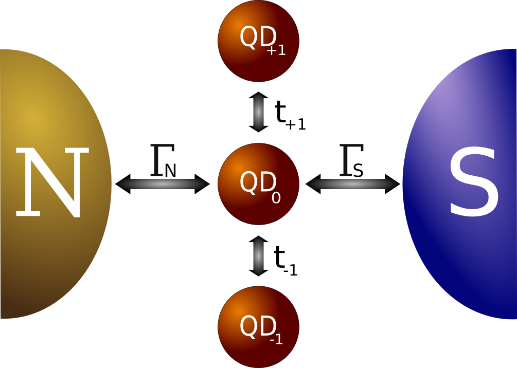
Figure 1: Schematic view of three quantum dots (QD_j) arranged vertically between the normal (N) and superconducting (S) electrodes. The central quantum dot, QD₀, is coupled by $\Gamma_{\beta}$ to the external reservoirs and by $t_{\pm 1}$ to the side-attached quantum dots, QD_±1.

The paper is organized as follows. In Sec. II we introduce the microscopic model and describe the method accounting for the induced electron pairing. Sec. III corresponds to the case of uncorrelated quantum dots in the deep subgap regime, studying evolution of the central quantum dot spectrum from the weak to strong interdot coupling. Next, in Sec. IV, we discuss the correlation effects in the subgap Kondo regime. Finally we summarize the results and present the conclusions.

II Microscopic model

The central quantum dot, QD₀, placed between the normal (N) and superconducting (S) electrodes and side-attached to the quantum dots, QD_±1, as shown in Fig. 1, can be modeled by the Anderson-type Hamiltonian

$$\hat{H}=\hat{H}_{QD}+\hat{H}_{N}+\hat{H}_{S}+\hat{H}_{QD-N}+\hat{H}_{QD-S}.$$ (1)

The set of three quantum dots can be described by

$$\hat{H}_{QD} = \sum_{\sigma,j}\epsilon_{j}\hat{d}^{\dagger}_{j\sigma}\hat{d}_{j\sigma}+\sum_{\sigma,{j=\pm 1}}\left(t_{j}\hat{d}^{\dagger}_{0\sigma}\hat{d}_{j\sigma}+\mbox{\rm h.c.}\right)$$ (2)

$$+ \sum_{j}U_{j}\hat{n}_{j\uparrow}\hat{n}_{j\downarrow},$$

where $\hat{d}_{j\sigma}^{(\dagger)}$ annihilates (creates) electron of $j$-th quantum dot with energy $\epsilon_{j}$ and spin $\sigma=\uparrow,\downarrow$. Hybridization between the quantum dots is characterized by the hopping integral $t_{\pm 1}$. We denote the number operator by $\hat{n}_{j\sigma}=\hat{d}_{j\sigma}^{\dagger}\hat{d}_{j\sigma}$ and $U_{j}$ stands for the Coulomb potential which is responsible for correlation effects.

We treat the normal (metallic) lead electrons as a free fermion gas $\hat{H}_{N}=\sum_{{\bf k},\sigma}\xi_{kN}\hat{c}^{\dagger}_{{\bf k}N\sigma}\hat{c}_{{\bf k}N\sigma}$ and describe the superconductor by the BCS model $\hat{H}_{S}=\sum_{{\bf k},\sigma}\xi_{{\bf k}S}\hat{c}^{\dagger}_{{\bf k}S\sigma}\hat{c}_{{\bf k}S\sigma}-\sum_{\bf k}\Delta\left(\hat{c}^{\dagger}_{{\bf k}S\uparrow}\hat{c}^{\dagger}_{-kS\downarrow}+{\mbox{\rm h.c.}}\right)$ with the isotropic energy gap $\Delta$. Operators $\hat{c}^{(\dagger)}_{{\bf k}\beta\sigma}$ refer to the mobile electrons of external ($\beta\!=\!N,S$) electrodes whose energies $\xi_{{\bf k}\beta}=\epsilon_{\bf k}-\mu_{\beta}$ are expressed with respect to the chemical potentials $\mu_{\beta}$. For convenience we choose $\mu_{S}=0$ as a reference level. Tunneling between the central dot and the external leads is described by $\hat{H}_{QD-\beta}=\sum_{{\bf k},\sigma}\left(V_{{\bf k}\beta}\hat{c}^{\dagger}_{{\bf k}\beta\sigma}\hat{d}_{0\sigma}+{\mbox{\rm h.c.}}\right)$, where $V_{{\bf k}\beta}$ denote the matrix elements. Focusing on the subgap quasiparticle states we apply the wide-band limit approximation, assuming the energy independent couplings $\Gamma_{\beta}=2\pi\sum_{\bf k}\left|V_{{\bf k}\beta}\right|^{2}\delta(\omega-\epsilon_{{\bf k}\beta})$.

II.1 Superconducting proximity effect

Measurable properties of our heterostructure predominantly depend on the effective spectrum of the central quantum dot, which results from: (i) the proximity induced pairing, (ii) electron correlations and (iii) influence of the side-attached quantum dots QD_±1. The superconducting proximity effect mixes the particle and hole degrees of freedom, therefore we have to introduce the matrix Green’s function

$${{\mbox{\boldmath{$G$}}}}_{j}(t,t^{\prime})=\begin{pmatrix}\langle\langle\hat{d}_{j\uparrow}(t);\hat{d}_{j\uparrow}^{\dagger}(t^{\prime})\rangle\rangle&\langle\langle\hat{d}_{j\uparrow}(t);\hat{d}_{j\downarrow}(t^{\prime})\rangle\rangle\\ \langle\langle\hat{d}_{j\downarrow}^{\dagger}(t);\hat{d}_{j\uparrow}^{\dagger}(t^{\prime})\rangle\rangle&\langle\langle\hat{d}_{j\downarrow}^{\dagger}(t);\hat{d}_{j\downarrow}(t^{\prime})\rangle\rangle\end{pmatrix},$$ (3)

where $\langle\langle\hat{A}(t);\hat{B}(t^{\prime})\rangle\rangle=-i\Theta(t\!-\!t^{\prime})\langle\left[\hat{A}(t),\hat{B}(t^{\prime})\right]\rangle$ is the retarded fermion propagator. In stationary case (for time-independent Hamiltonian) the Green’s function (3) depends on $t\!-\!t^{\prime}\equiv\tau$ and its Fourier transform ${{\mbox{\boldmath{$G$}}}}_{j}(\omega)\equiv\int d\tau e^{-i\omega\tau}{{\mbox{\boldmath{$G$}}}}_{j}(\tau)$ obeys the Dyson equation

$$\left[{{\mbox{\boldmath{$G$}}}}_{j}(\omega)\right]^{-1}=\begin{pmatrix}\omega-\epsilon_{j}&0\\ 0&\omega+\epsilon_{j}\end{pmatrix}-{{\mbox{\boldmath{$\Sigma$}}}}_{j}(\omega).$$ (4)

The selfenergy matrix ${{\mbox{\boldmath{$\Sigma$}}}}_{j}(\omega)$ describes influence of the inter-dot couplings, the external leads, and the correlations. In general, its analytic form is unknown.

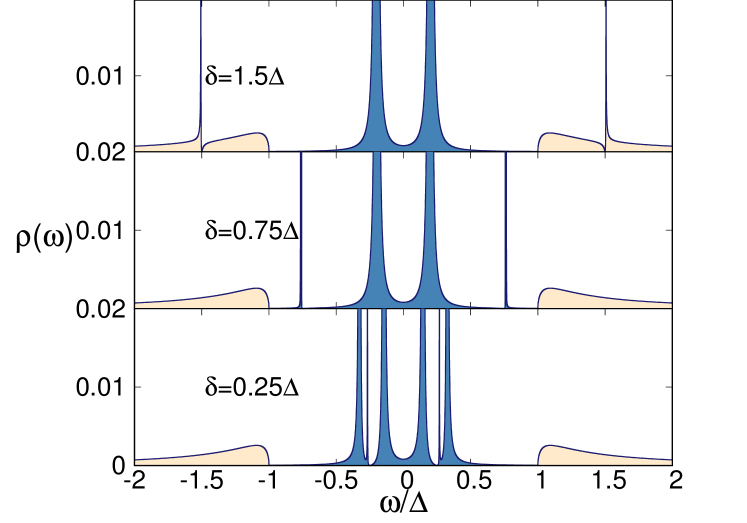
Figure 2: Spectral function $\rho(\omega)$ [in units of $\frac{2}{\pi\Gamma_{N}}$] of the central dot obtained for $\epsilon_{0}=0$, $\Gamma_{S}/\Delta=0.5$, $\Gamma_{N}/\Delta=0.01$, $U_{0}=0$, $t/\Delta=0.15$ and representative detunings: $\delta/\Delta=1.5$ (top), $0.75$ (middle), $0.25$ (bottom panel).

II.2 Features of a weak inter-dot coupling

It is instructive to analyze first how the side-attached quantum dots come along with the proximity induced electron pairing, neglecting the correlations $U_{j}=0$. The selfenergy of uncorrelated QD₀ is given by

$${{\mbox{\boldmath{$\Sigma$}}}}^{U=0}_{0}(\omega) = \begin{pmatrix}\frac{-i\Gamma_{N}}{2}-\frac{i\Gamma_{S}}{2}\tilde{\rho}(\omega)&-\frac{i\Gamma_{S}}{2}\tilde{\rho}(\omega)\frac{\Delta}{\omega}\\ -\frac{i\Gamma_{S}}{2}\tilde{\rho}(\omega)\frac{\Delta}{\omega}&\frac{-i\Gamma_{N}}{2}-\frac{i\Gamma_{S}}{2}\tilde{\rho}(\omega)\end{pmatrix}$$ (5)

$$+ \sum_{j=\pm 1}\begin{pmatrix}\frac{t_{j}^{2}}{\omega-\epsilon_{j}}&0\\ 0&\frac{t_{j}^{2}}{\omega+\epsilon_{j}}\end{pmatrix},$$

where

$$\tilde{\rho}(\omega)=\left\{\begin{array}[]{ll}\frac{\omega}{\sqrt{\Delta^{2}-\omega^{2}}}&\mbox{\rm for }|\omega|\leq\Delta,\\ \frac{i\;|\omega|}{\sqrt{\omega^{2}-\Delta^{2}}}&\mbox{\rm for }|\omega|>\Delta.\end{array}\right.$$ (6)

Let us inspect the spectral function of QD₀

$$\rho(\omega)=-\frac{1}{\pi}\;\mbox{\rm Im}\left\{G_{0,11}(\omega+i0^{+})\right\},$$ (7)

assuming the side-attached quantum dots to be weakly coupled to the central dot. Following the previous studies of three quantum dots on interface between two metallic electrodes trocha2008a ; trocha2008b ; vernek2010 we impose $t_{-1}=t_{+1}\equiv t$ and define the energy detuning $\epsilon_{+1}-\epsilon_{0}=\epsilon_{0}-\epsilon_{-1}\equiv\delta$. Figure 2 shows $\rho(\omega)$ for the asymmetric couplings $\Gamma_{S}>\Gamma_{N}$, when the quasiparticle states of the subgap regime (marked by blue color in Fig. 2) are sufficiently narrow (long-lived). For the large detuning $\delta>\Delta$ (top panel) we observe two Fano-type resonances appearing outside the superconducting gap at $\omega=\pm\delta$. For the moderate detuning $\delta=0.75\Delta$ (middle panel) there appear some features inside the superconducting gap, but they no longer resemble Fano-type lineshapes. For the very small detuning $\delta=0.25\Delta$ (bottom panel), a rather complicated subgap structure emerges. To clarify its physical origin, we explore in section III the deep subgap regime $|\omega|\ll\Delta$.

III Subgap Dicke effect vs pairing

In this part we study in more detail the extreme subgap region $|\omega|\ll\Delta$, for which the selfenergy (5) simplifies to

$$\lim_{|\omega|\ll\Delta}{{\mbox{\boldmath{$\Sigma$}}}}^{U\!=\!0}_{0}(\omega)=\begin{pmatrix}\frac{-i\Gamma_{N}}{2}+\sum_{j}\frac{t_{j}^{2}}{\omega-\epsilon_{j}}&-\frac{\Gamma_{S}}{2}\\ -\frac{\Gamma_{S}}{2}&\frac{-i\Gamma_{N}}{2}+\sum_{j}\frac{t_{j}^{2}}{\omega+\epsilon_{j}}\end{pmatrix}$$ (8)

with summation running over $j=\pm 1$. The presence of the superconducting reservoir shows up in the selfenergy (8) through the static off-diagonal terms, which can be interpreted as the induced on-dot pairing potential Bauer-2007 .

III.1 From interferometric to molecular regions

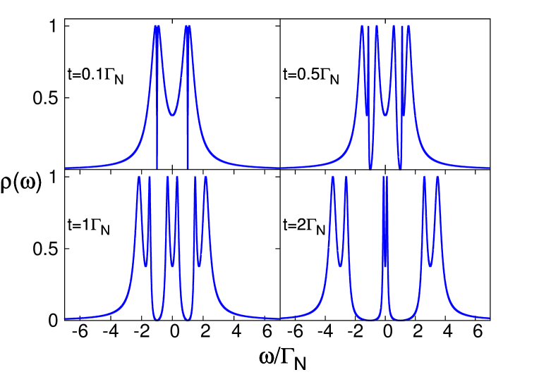
Figure 3: Electronic spectrum of QD₀ obtained for $\Gamma_{S}=2\Gamma_{N}$, $\delta=\Gamma_{N}$, $U_{j}=0$, $\varepsilon_{0}=0$ and various interdot couplings $t$.

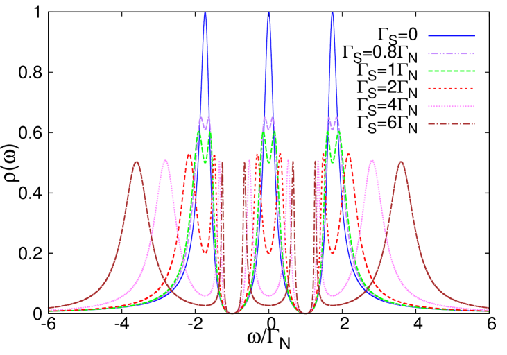
Figure 4: Spectral function $\rho(\omega)$ of the uncorrelated QD₀ obtained in the molecular region $t=\Gamma_{N}$ for $\delta=\Gamma_{N}$, $\varepsilon_{0}=0$, $U_{j}=0$ and various couplings $\Gamma_{S}$, as indicated.

Figure 3 presents the spectral function $\rho(\omega)$ obtained for $\Gamma_{S}=2\Gamma_{N}$ and several values of the interdot coupling, ranging from the interferometric (small $t$) to the molecular (large $t$) regimes. For the weak coupling $t=0.1\Gamma_{N}$ we observe the Fano-type lineshapes at $\epsilon_{\pm 1}$ appearing on top of the Andreev quasiparticles that are centered at $\pm\sqrt{\epsilon_{0}^{2}+(\Gamma_{S}/2)^{2}}$. With increasing $t$ the spectrum gradually evolves to the ‘molecular’ structure, characterized by the subradiant (narrow central) quasiparticle and superradiant (broad side-peaks) states. Similar tendency has been reported for the heterojunction with both normal leads trocha2008a ; trocha2008b ; vernek2010 . In the present case, however, we observe additional qualitative changes caused by the proximity effect. Figure 4 shows the evolution of the spectral function $\rho(\omega)$ with respect to $\Gamma_{S}$. At some critical coupling $\Gamma_{S}\approx 0.6\Gamma_{N}$ the sub- and superradiant states effectively split due to the on-dot electron pairing. We denote these splittings by $\Delta_{c}$ for the central peak and by $\Delta_{s}$ for the side peaks, respectively. Their magnitudes are displayed in Fig. 5.

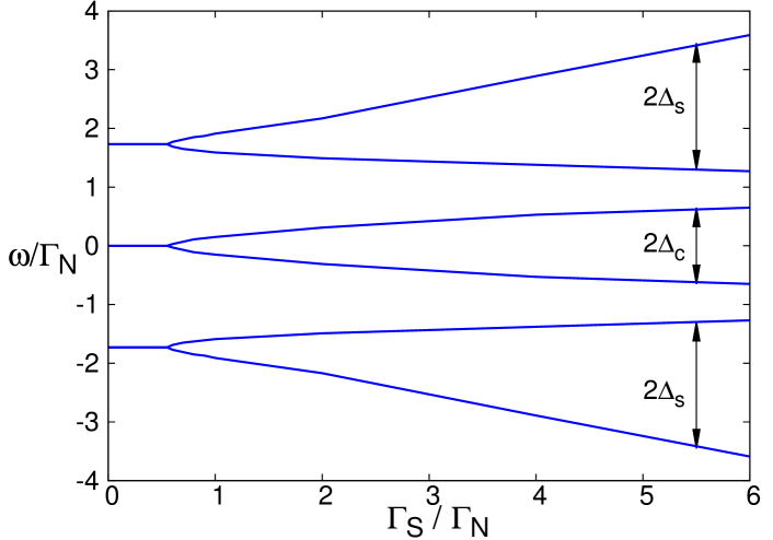
Figure 5: Splitting of the subradiant ($\Delta_{c}$) and superradiant ($\Delta_{s}$) quasiparticle states caused by the superconducting proximity effect for $t=\Gamma_{N}$, $\delta=\Gamma_{N}$, $\varepsilon_{0}=0$, $U_{j}=0$.

We notice, that particle-hole splitting of the central (subradiant) peak differs from the corresponding effect in the side (superradiant) peaks, see the upper panel of Fig. 6 which shows the spectral function of the middle quantum dot QD₀. Symmetric shape of the subradiant quasiparticle is perfectly preserved, but with increasing $\Gamma_{S}$ its internal splitting is bounded from above ($\Delta_{c}\rightarrow\delta$). Such limitation comes from the destructive quantum interference, which depletes the electronic states around $\epsilon_{\pm 1}$. On the other hand, the superradiant quasiparticle peaks are not much affected by any constraints, therefore $\Delta_{s}$ monotonously grows with increasing $\Gamma_{S}$. We observe, however, that such superradiant states acquire asymmetric shape with the narrow structure slightly outside $|\epsilon_{\pm 1}|$ and another broader peak in the high energy regime. In the extremely strong $\Gamma_{S}$ coupling limit, the high energy peaks absorb majority of the spectral weight.

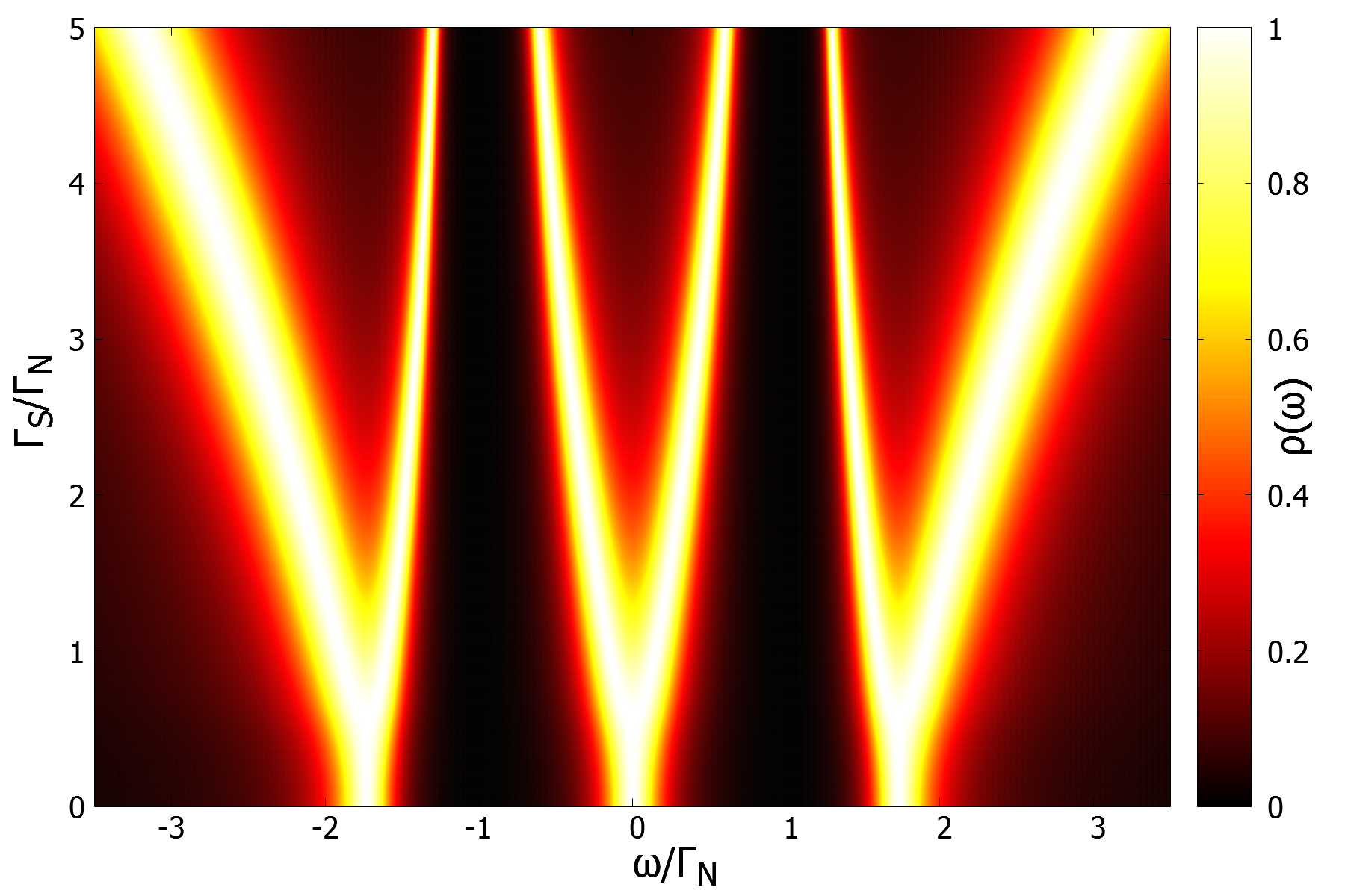
Figure 6: Electronic spectrum of the central QD₀ in the molecular $t=1\Gamma_{N}$ (upper panel) and interferometric $t=0.15\Gamma_{N}$ (bottom panel) regions obtained for $U_{j}=0$, $\varepsilon_{0}=0$, $\delta=\Gamma_{N}$.

On the other hand, in the interferometric regime (see bottom panel in Fig. 6) we observe the Andreev quasiparticle states (centered around $\pm\Gamma_{S}/2$ and their broadening equal $\Gamma_{N}$) with the Fano-type lineshapes appearing at $\omega=\epsilon_{\pm 1}$. Total spectral weight contained in the regime $\omega\in\left[\epsilon_{-1},\epsilon_{+1}\right]$ is gradually washed out with increasing $\Gamma_{S}$. Such transfer of the spectral weight for the molecular and interferometric cases is displayed in Fig. 7. In both cases the induced electron pairing depletes the low-energy quasiparticle states by transferring their spectral weight towards the higher energy quasiparticle states. Section IV shows that this process constructively affects the Kondo effect.

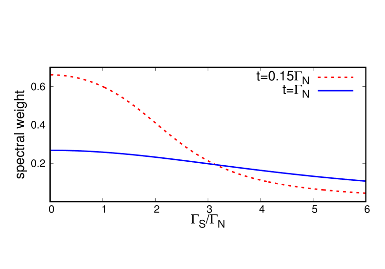
Figure 7: Spectral weight of the low energy electronic states for $\omega\in\left[\epsilon_{-1},\epsilon_{+1}\right]$ caused by the electron pairing for the interferometric (dashed line) and molecular (solid line) regions.

III.2 Subgap tunneling conductance

Any experimental verification of the subgap energy spectrum can be performed by measuring the tunneling current, induced under nonequilibrium conditions $\mu_{N}-\mu_{S}=eV$ (where $V$ is an applied voltage). At low voltage the subgap current is provided solely by the anomalous Andreev channel, when electrons are scattered back to $N$ electrode as holes, injecting the Copper pairs to superconducting electrode. Within the Landauer approach such current can be expressed by

$$I(V)=\frac{2e}{h}\int d\omega\;T_{A}(\omega)\left[f_{FD}(\omega-eV)-f_{FD}(\omega+eV)\right],$$

where $f_{FD}(\omega)=\left[1+\mbox{\rm exp}\left(\omega/k_{B}T\right)\right]^{-1}$ is the Fermi-Dirac distribution function. The Andreev transmittance $T_{A}(\omega)=\Gamma_{N}^{2}\left|{{\mbox{\boldmath{$G$}}}}_{0,12}(\omega)\right|^{2}$ is a quantitative measure of the proximity induced pairing which indirectly probes the subgap electronic spectrum, although in a symmetrized manner, because the particle and hole degrees of freedom equally contribute to such transport channel.

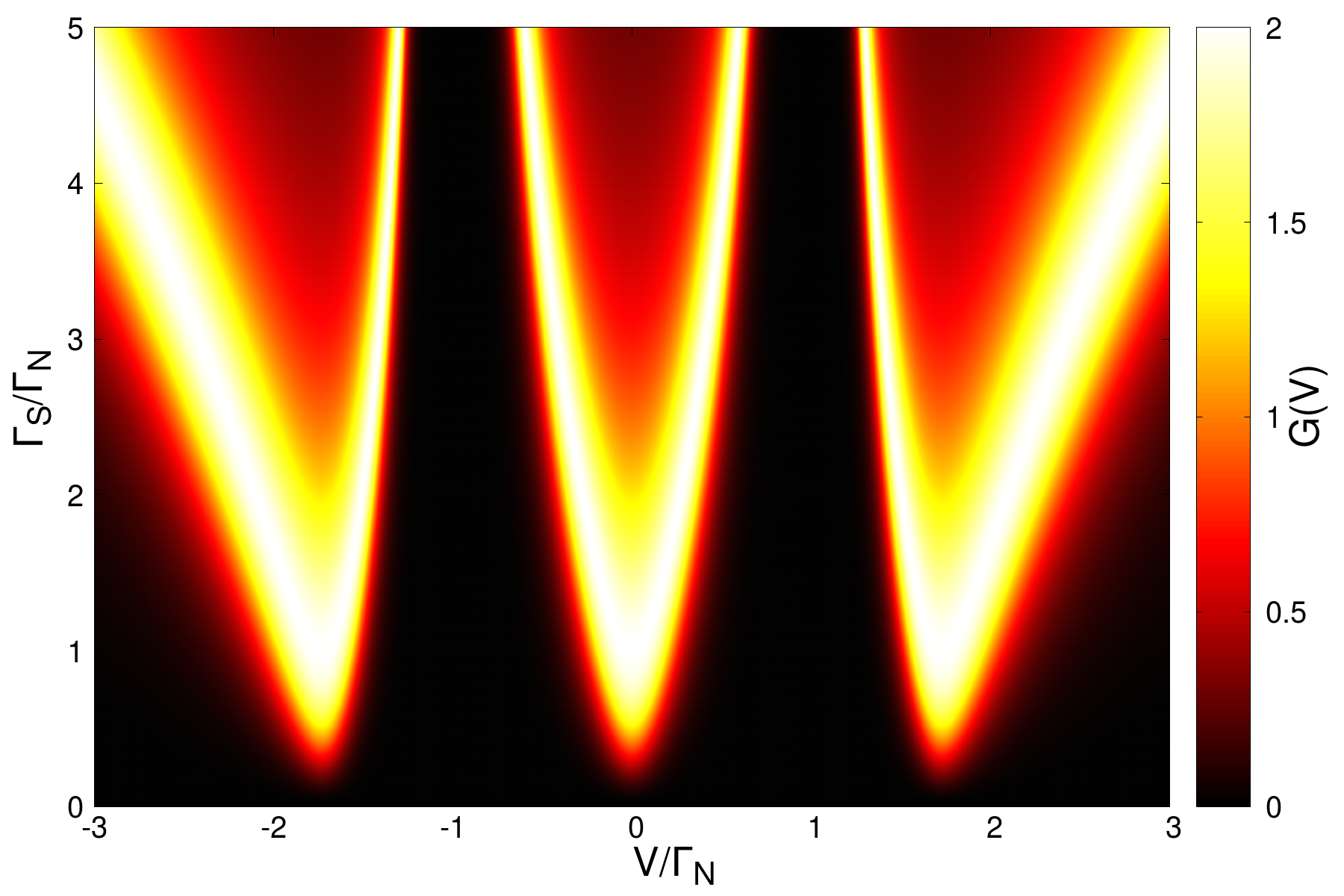
Figure 8: The differential Andreev conductance $G(V)$ [in units of $2e^{2}/h$] obtained for the same model parameters as in Fig. 6.

Figure 8 shows the differential Andreev conductance $G(V)=dI(V)/dV$ obtained for the uncorrelated quantum dots. We can notice, that the subgap transport properties are sensitive to both the quantum interference (for small $t$) or the Dicke-like effect (for the strong interdot coupling). The optimal conductance $4e^{2}/h$ occurs at such voltages $V$, which coincide with the subgap quasiparticle energies. The Andreev spectroscopy would thus be able to verify the aforementioned relationship of the interferometric and/or Dicke effect with the proximity induced electron pairing.

IV Interplay with Kondo effect

Repulsive interactions $U_{j}$ between opposite spin electrons can induce further important effects. It is convenient to describe their influence, expressing the matrix Green’s function ${{\mbox{\boldmath{$G$}}}}_{j}(\omega)$ via Bauer-2007 ; Li-2016

$${{\mbox{\boldmath{$G$}}}}_{j}(\omega)={{\mbox{\boldmath{$G$}}}}_{j}^{0}(\omega)+{{\mbox{\boldmath{$G$}}}}_{j}^{0}(\omega)\;U_{j}\;{{\mbox{\boldmath{$F$}}}}_{j}(\omega),$$ (9)

where ${{\mbox{\boldmath{$G$}}}}_{j}^{0}(\omega)$ refers to the case $U_{j}=0$, and the two-body Green’s function ${{\mbox{\boldmath{$F$}}}}_{j}(\omega)$ is defined as

$${{\mbox{\boldmath{$F$}}}}_{j}(\omega)=\begin{pmatrix}\langle\langle\hat{d}_{j\uparrow}\hat{n}_{j\downarrow};\hat{d}_{j\uparrow}^{\dagger}\rangle\rangle&\langle\langle\hat{d}_{j\uparrow}\hat{n}_{j\downarrow};\hat{d}_{j\downarrow}\rangle\rangle\\ \langle\langle-\hat{d}_{j\downarrow}^{\dagger}\hat{n}_{j\uparrow};\hat{d}_{j\uparrow}^{\dagger}\rangle\rangle&\langle\langle-\hat{d}_{j\downarrow}^{\dagger}\hat{n}_{j\uparrow};\hat{d}_{j\downarrow}\rangle\rangle\end{pmatrix}.$$ (10)

In this paper we focus on the correlation effects driven by the potential $U_{0}$, because it has the predominant influence on measurable transport properties of our system. As concerns $U_{\pm 1}$, they could merely mimic the multilevel structure of the side-coupled dots. In experimental realizations of the correlated quantum dots coupled to the superconducting electrodes deacon2010 ; lee2012 ; pillet2013 ; Zitko-2015 the Coulomb potential $U_{j}$ usually exceeds the superconducting energy gap $\Delta$ (at least by one order of magnitude). Under such circumstances the correlation effects manifest themselves in the subgap regime $|\omega|<\Delta$ in a rather peculiar way, via (i) the singlet-doublet transition (or crossover) and (ii) the subgap Kondo effect Zitko-2015 ; Domanski-2016 .

IV.1 Perturbative approach

The singlet-doublet transition can be captured already within the lowest order (Hartree-Fock-Bogoliubov) decoupling scheme

$$U_{0}{{\mbox{\boldmath{$F$}}}}_{0}(\omega)\approx\underbrace{U_{0}\begin{pmatrix}\langle\hat{n}_{0\downarrow}\rangle&\langle\hat{d}_{0\downarrow}\hat{d}_{0\uparrow}\rangle\\ \langle\hat{d}_{0\uparrow}^{\dagger}\hat{d}_{0\downarrow}^{\dagger}\rangle&-\langle\hat{n}_{0\uparrow}\rangle\end{pmatrix}}_{\Sigma_{0}^{1st}}{{\mbox{\boldmath{$G$}}}}_{0}(\omega).$$ (11)

As usually the 1-st order correction (with respect to $U_{0}$) to the selfenergy is static, therefore it can be incorporated into the renormalized energy level $\tilde{\epsilon}_{0}\equiv\epsilon_{0}+U_{0}\langle\hat{n}_{0\sigma}\rangle$ and the effective pairing potential $\tilde{\Gamma}_{S}/2\equiv\Gamma_{S}/2-U_{0}\langle\hat{d}_{0\downarrow}\hat{d}_{0\uparrow}\rangle$. Such Hartree-Fock-Bogoliubov corrections (11) imply a crossing of the subgap Andreev states when the ground state changes from the spinful to spinless configuration upon increasing the ratio of $\Gamma_{S}/U_{0}$. This effect is known to reverse the tunneling current in the Josephson junctions (so called, $0-\pi$ transition) and has been extensively studied (see Ref. [Zonda-2015, ] for a comprehensive discussion).

To describe the subgap Kondo effect it is, however, necessary to go beyond the mean field approximation (11), taking into account the higher order (dynamic) corrections

$$U_{0}{{\mbox{\boldmath{$F$}}}}_{0}(\omega)=\left[{{\mbox{\boldmath{$\Sigma$}}}}_{0}^{1st}+{{\mbox{\boldmath{$\Sigma$}}}}_{0}^{dyn}(\omega)\right]{{\mbox{\boldmath{$G$}}}}_{0}(\omega).$$ (12)

Formally, Eq. (12) can be recast into the Dyson form ${{\mbox{\boldmath{$G$}}}}_{0}(\omega)^{-1}={{\mbox{\boldmath{$G$}}}}^{0}_{0}(\omega)^{-1}-\left[{{\mbox{\boldmath{$\Sigma$}}}}_{0}^{1st}+{{\mbox{\boldmath{$\Sigma$}}}}_{0}^{dyn}(\omega)\right]$. Obviously the dynamic part ${{\mbox{\boldmath{$\Sigma$}}}}_{0}^{dyn}(\omega)$ can be estimated only approximately, because the present problem is not solvable.

In the limit $|\omega|\ll\Delta$ the diagonal and off-diagonal parts of the Green’s function ${{\mbox{\boldmath{$G$}}}}_{0}(\omega)$ are interdependent through the (exact) relation Bauer-2007

$$\left(\tilde{\omega}-\epsilon_{0}\right){{\mbox{\boldmath{$G$}}}}_{0,11}(\omega)=1-\frac{\Gamma_{S}}{2}{{\mbox{\boldmath{$G$}}}}_{0,21}(\omega)+U_{0}{{\mbox{\boldmath{$F$}}}}_{0,11}(\omega).$$ (13)

Here $\tilde{\omega}=\omega-\sum_{{\bf k}}\frac{|V_{{\bf k}N}|^{2}}{\omega\!-\!\xi_{{\bf k}N}}$, which in the wide-band limit simplifies to $\tilde{\omega}=\omega+i\Gamma_{N}/2$. We determine the two-body propagator ${{\mbox{\boldmath{$F$}}}}_{0,11}(\omega)=\langle\langle\hat{d}_{0\uparrow}\hat{n}_{0\downarrow};\hat{d}_{0\uparrow}^{\dagger}\rangle\rangle$ using the decoupling scheme within the equation of motion procedure EOM-method

$${{\mbox{\boldmath{$F$}}}}_{0,11}(\omega)\simeq\frac{\langle\hat{n}_{0\downarrow}\rangle-\gamma_{1}(\omega)\;{{\mbox{\boldmath{$G$}}}}_{0,11}(\omega)}{\tilde{\omega}-\epsilon_{0}-U_{0}-\gamma_{3}(\omega)},$$ (14)

where the auxiliary functions $\gamma_{\nu}(\omega)$ are defined as

$$\gamma_{\nu}(\omega) = \sum_{{\bf k}}\!\left[\frac{|V_{{\bf k}N}|^{2}}{\omega\!-\!\xi_{{\bf k}N}}+\frac{|V_{{\bf k}N}|^{2}}{\omega\!-\!U_{0}\!-2\varepsilon_{0}\!+\!\xi_{{\bf k}N}}\right]$$ (17)

$$\times \left\{\begin{array}[]{lc}f_{FD}(\xi_{{\bf k}N})&\mbox{\rm for }\nu=1,\\ 1&\mbox{\rm for }\nu=3.\end{array}\right.$$

This method implies the diagonal selfenergy ${{\mbox{\boldmath{$\Sigma$}}}}_{0,11}(\omega)={{\mbox{\boldmath{$\Sigma$}}}}_{0,11}^{1st}+{{\mbox{\boldmath{$\Sigma$}}}}_{0,11}^{dyn}(\omega)$ in the familiar form EOM-method

$$\frac{1}{\omega-\epsilon_{0}-{{\mbox{\boldmath{$\Sigma$}}}}_{0,11}(\omega)} = \frac{1-\langle\hat{n}_{0\downarrow}\rangle}{\tilde{\omega}-\epsilon_{0}+\frac{U_{0}\gamma_{1}(\omega)}{\tilde{\omega}-\epsilon_{0}-U_{0}-\gamma_{3}(\omega)}}$$

$$+ \frac{\langle\hat{n}_{0\downarrow}\rangle}{\tilde{\omega}-\epsilon_{0}-U_{0}+\frac{U_{0}[\gamma_{1}(\omega)-\gamma_{3}(\omega)]}{\tilde{\omega}-\epsilon_{0}-\gamma_{3}(\omega)}}.$$

The off-diagonal term ${{\mbox{\boldmath{$\Sigma$}}}}_{0,21}(\omega)$ can be obtained from Eqs. (13) and (14). Such procedure provides the qualitative insight into the Kondo effect, spectroscopically manifested by the narrow Abrikosov-Suhl peak at $\omega=\mu_{N}$.

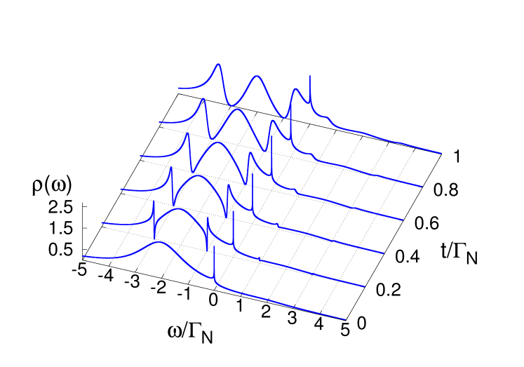
Figure 9: Evolution of the spectral function $\rho(\omega)$ obtained for the strongly correlated QD₀ in the Kondo region from the interferometric (small $t$) to molecular (large $t$) limits. Calculations have been done for $\mu_{N}=0$, $\epsilon_{0}=-2\Gamma_{N}$, $\delta=\Gamma_{N}$, $\Gamma_{S}=4\Gamma_{N}$ and $U_{0}=100\Gamma_{N}$.

We now investigate the effect of the interdot coupling on the Andreev spectroscopy, considering the interferometric and the molecular regions. Figure 9 shows the spectrum of QD₀ in the Kondo regime at temperature $T=10^{-6}\Gamma_{N}$ for $\epsilon_{0}=-2\Gamma_{N}$, $\delta=\Gamma_{N}$, $\Gamma_{S}=4\Gamma_{N}$, assuming the large Coulomb potential $U_{0}=100\Gamma_{N}$. Initially, for $t=0$, the spectral function $\rho(\omega)$ reveals: (i) the quasiparticle peak at $\omega\approx\epsilon_{0}$, (ii) its tiny particle-hole companion at $\omega\approx-\epsilon_{0}$ (let us remark that superconducting proximity effect substantially weakens upon increasing $|\epsilon_{0}|/\Gamma_{S}$) and (iii) the narrow Abrikosov-Suhl peak at $\omega=\mu_{N}$ (manifesting the Kondo effect). For the weak interdot coupling $t\ll\Gamma_{N}$, we notice appearance of the Fano-type (interferometric) features at $\omega=\epsilon_{\pm 1}$. For the stronger coupling $t$, the spectrum of QD₀ evolves to its molecular-like structure, resembling the one discussed in the preceding section. Upon increasing $t$, the subradiant quasiparticle (centered around $\epsilon_{0}$) gradually narrows, whereas the superradiant quasiparticles absorb more and more spectral weights. Such transfer of the spectral weight indirectly amplifies the Abrikosov-Suhl peak, existing on the upper superradiant quasiparticle.

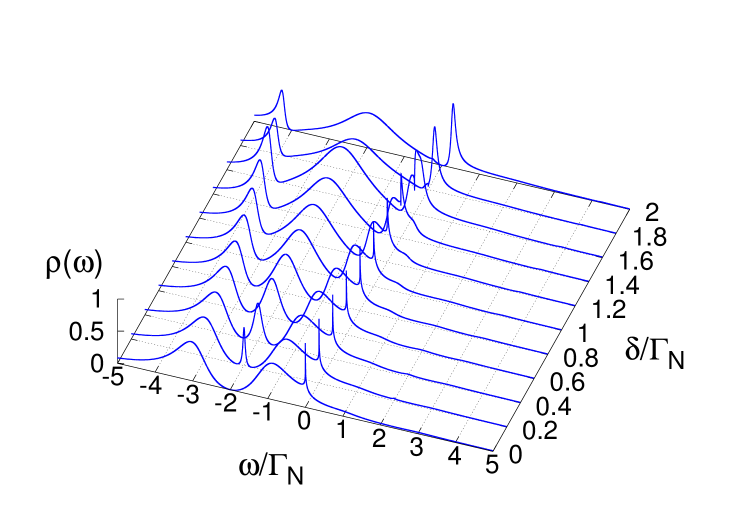
Figure 10: Spectral function of the correlated central quantum dot in the Kondo regime obtained for $t=2\Gamma_{N}$ using $\epsilon_{0}=-2\Gamma_{N}$, $\Gamma_{S}=4\Gamma_{N}$, $U_{0}=100\Gamma_{N}$.

In the discussed case the Dicke effect constructively amplifies the Abrikosov-Suhl peak, but in general the Kondo effect can depend on the detuning $\delta$. This is illustrated in Fig. 10, where upon varying $\epsilon_{\pm 1}-\epsilon_{0}$ the Abrikosov-Suhl peak is enhanced up to some critical detuning $\delta_{crit}\sim t$, at which destructive interference depletes all the electronic states near $\mu_{N}$.

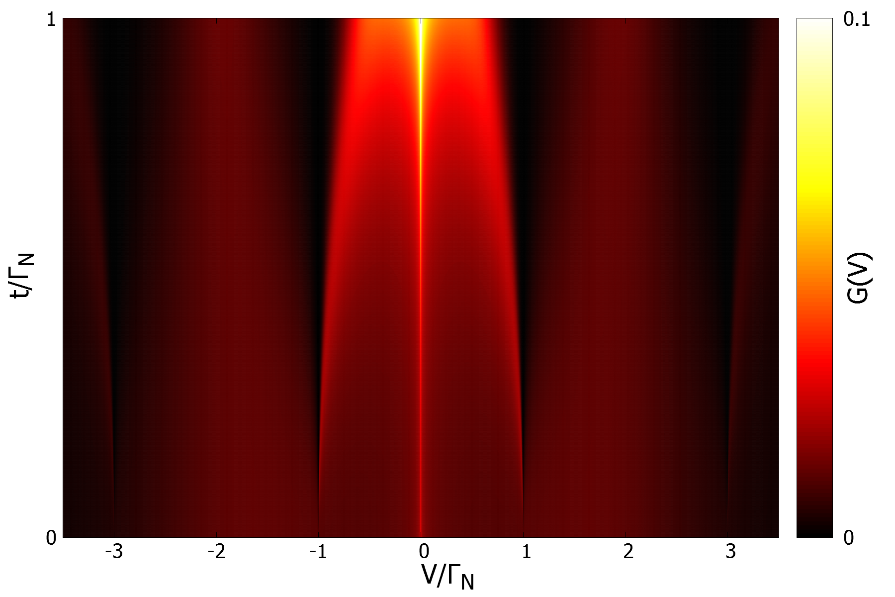
Figure 11: The differential Andreev conductance $G(V)=dI(V)/dV$ [in units $2e^{2}/h$] as a function of the interdot coupling $t$, ranging from the weak (interferometric) to molecular (Dicke) regions. Calculations have been done for the same model parameters as in Fig. 9.

In Fig. 11 we show the differential Andreev conductance obtained for our setup at temperature $T=10^{-6}\Gamma_{N}$ as a function of the voltage $V$ and the interdot coupling $t$. In the absence of the side-attached dots ($t=0$) we notice two broad maxima at $|eV|\approx\epsilon_{0}$ (corresponding to energies of the subgap quasiparticle states) and the zero-bias peak (due to the Kondo effect). For finite and weak interdot coupling $t\ll\Gamma_{N}$, the quantum interference starts to play a role as manifested by the asymmetric Fano-type resonances at $\epsilon_{\pm 1}$. With further increase of $t$ we observe development of the sub- and superradiant features, typical for the molecular regime. Transfer of the spectral weight from the subradiant to superradiant states amplifies the zero-bias conductance (bright region at $V\sim 0$).

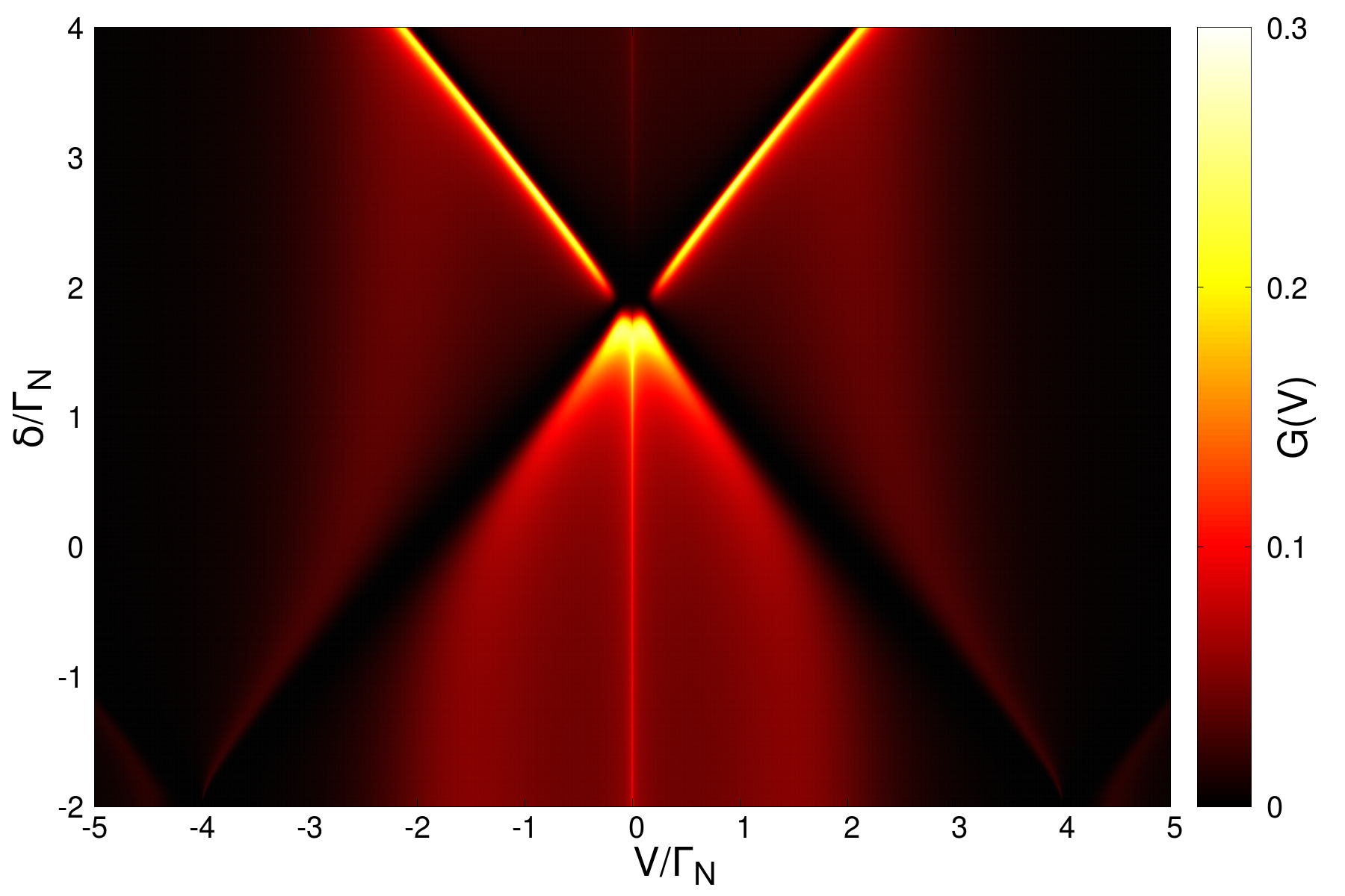
Figure 12: The differential Andreev conductance $G(V)$ versus $\delta$ obtained for the same set of parameters used in Fig. 10.

Figure 12 shows the evolution of the differential Andreev conductance with respect to $\delta$ for the same set of parameters as used in Fig. 10. Since the zero-bias conductance probes the quasiparticle states at $\omega\sim 0$, it tells us (indirectly) about behavior of the subgap Kondo effect. The ongoing redistribution of the spectral weight between the subradiant and superradiant states enhances this zero-bias conductance until the critical detuning $\delta_{c}\approx t$. Above this critical detuning, the Kondo effect is completely washed out, signaling qualitative change of the QD₀ ground state. For a better understanding of the low energy physics, we perform nonperturbative calculations based on the numerical renormalization group (NRG) technique.

IV.2 NRG results

For a reliable analysis of a subtle interplay between the correlations, the induced electron pairing, and the sub/super-radiant Dicke states we performed the numerical renormalization group calculations Wilson . Our major concern was to investigate the low energy Kondo physics appearing in the sub-gap regime due to the spin-exchange interactions between the central quantum dot and the metallic lead Domanski-2016 . In such deep subgap regime (8) the quantum dot hybridized with the superconducting reservoir can be described by the effective Hamiltonian Bauer-2007 ; RozhkovArovas

$$\hat{H}_{QD}+\hat{H}_{S}+\hat{H}_{QD-S}\rightarrow\hat{H}_{QD}-\frac{\Gamma_{S}}{2}\left(\hat{d}^{\dagger}_{0\uparrow}\hat{d}^{\dagger}_{0\downarrow}+\hat{d}_{0\downarrow}\hat{d}_{0\uparrow}\right).$$

Under such conditions the initial Hamiltonian (1) simplifies to the single-channel model, allowing for a vast reduction of computation efforts. We performed NRG calculations, using the Budapest Flexible DM-NRG code fnrg for constructing the density matrix of the systemAndersSchiller ; dm-nrg and determining the matrix Green’s function (3). During the calculations we exploited the spin SU(2) symmetry and kept $N_{\rm kept}=3000$ multiplets. We obtained the satisfactory solution within $N=50$ iterative steps, assuming a flat density of states of the normal lead with a cutoff $D=U_{0}$ and imposing the discretization parameter $\Lambda=2$. To improve the quality of the spectral data, our results were averaged over $N_{z}=4$ interleaved discretizations Z . Next, we determined the real parts of ${\mbox{\boldmath{$G$}}}(\omega)$ [needed for the Andreev transmittance] from the Kramers-Krönig relations.

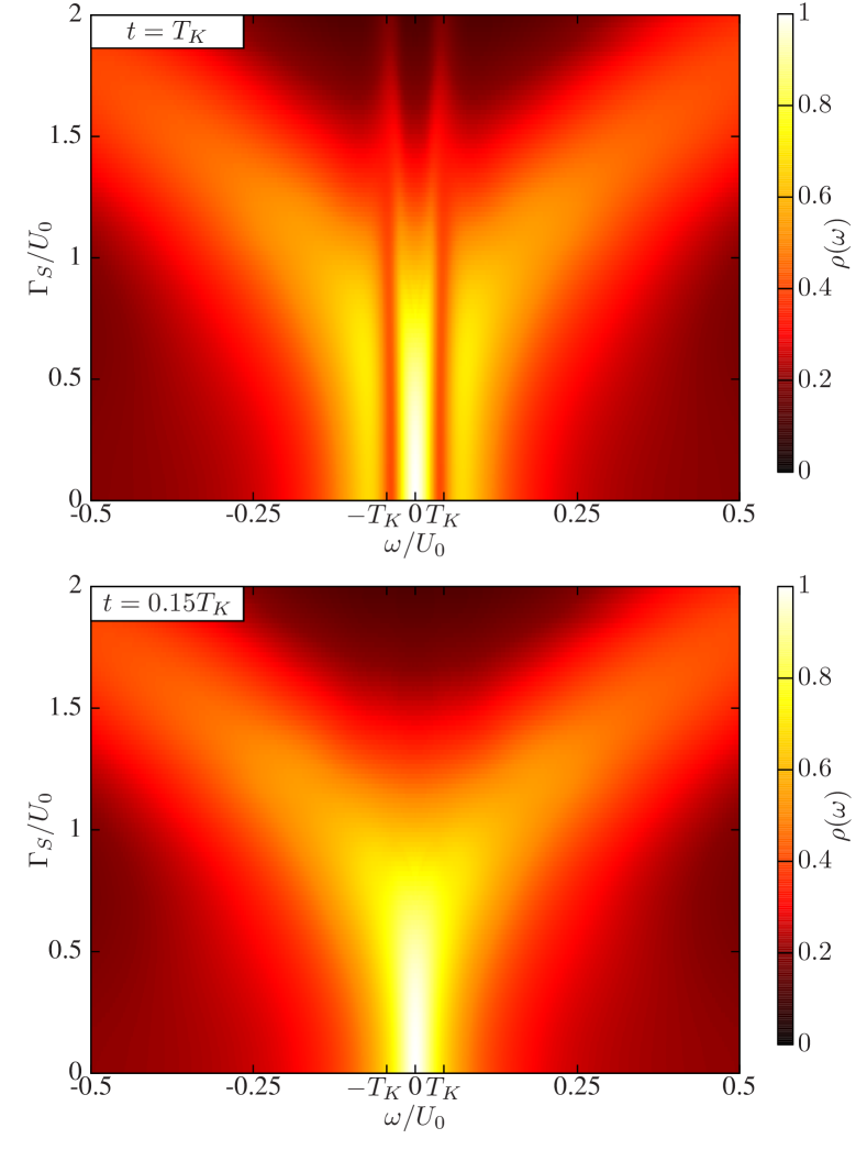
Figure 13: The spectral function of the half-filled QD₀ obtained by NRG for $\Gamma_{N}=0.4U_{0}$, $\delta=T_{K}=0.044U_{0}$, $T=0$, and $t=\delta$ (top panel) or $t=0.15\delta$ (bottom panel).

Figure 13 presents the spectral function obtained by NRG for QD₀ using $\Gamma_{N}=0.4U_{0}$ and $\delta=T_{K}=0.044U_{0}$, where the Kondo temperature $T_{K}$ is estimated with the Haldane formula Haldane in the case of $t=\Gamma_{S}=0$. For $t=\delta$, some similarities to the bottom panel of Fig. 6 can be observed. First of all, for $\Gamma_{S}=0$, the spectral function $\rho(\omega)$ exhibits a peak at $\omega=0$ and two side peaks at frequencies $\omega\approx\pm\delta$. When $\delta=T_{K}$, the side peaks are very close to the central one and are definitely less sharp than for the non-interacting case presented in Fig. 6. For $\Gamma_{S}\gtrsim U_{0}$, the Abrikosov-Suhl peak smoothly evolves into the Andreev quasiparticle states Domanski-2016 and the spectral weight is successively shifted towards the side peaks. For stronger coupling $\Gamma_{S}$, the Kondo effect is no longer present.

For $t=0.15T_{K}$, the situation is rather different (bottom panel of Fig. 13) because instead of the Dicke effect we can see only some interferometric signatures. For small $\Gamma_{S}$, the spectral function is characterized by the single Abrikosov-Suhl peak. With increasing $\Gamma_{S}$ such peak gradually broadens, and finally for $\Gamma_{S}\gtrsim U_{0}$ it splits because of a quantum phase transition from the spinful (doublet) to the spinless (singlet) configurations Bauer-2007 ; Domanski-2016 . We presume that the inter-dot coupling $t=0.15T_{K}$ is too weak to have any significant influence on the low-energy properties of our system (unlike the case considered in the bottom panel of Fig. 6). Yet, the spectral weight transfer towards the higher energies with increasing $\Gamma_{S}$ is quite evident.

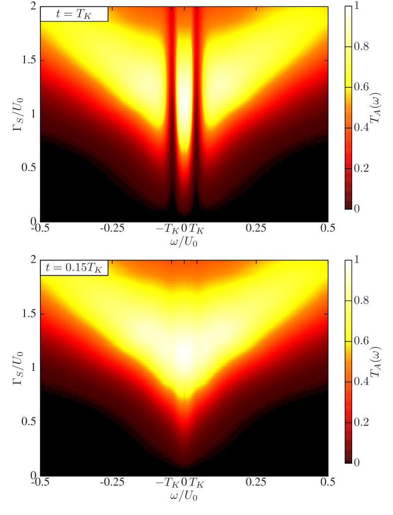
Figure 14: The Andreev transmittance $T_{A}(\omega)$ obtained by NRG for the set of model parameters corresponding to Fig. 13.

The observations shown in Fig. 13 have their consequences for the measurable transport quantities. Results for the zero-temperature Andreev transmittance $T_{A}(\omega)$ obtained by the NRG calculations are presented in Fig. 14. At zero temperature, the Andreev transmittance has a simple relationship with the differential conductance $G(V)=\frac{2e^{2}}{h}[T_{A}(\omega=eV)+T_{A}(\omega=-eV)]$. For small $\Gamma_{S}$, the energetically favorable ground state configuration of QD₀ is $\left|\sigma\right>$, therefore it is hardly affected by the superconducting proximity effect, hence the Andreev transmittance [dependent on the off-diagonal terms of the matrix Green’s function ${\mbox{\boldmath{$G$}}}_{0}(\omega)$] is negligibly small. With increasing $\Gamma_{S}$ the central quantum dot evolves to the BCS-type configuration $v\left|0\right>-u\left|\uparrow\downarrow\right>$, therefore efficiency of the pairing effects is significantly enhanced as can be seen by bright areas in Fig. 14 for $\Gamma_{S}\gtrsim U_{0}$. Such changeover of the QD₀ ground state is, however, detrimental to the Kondo effect because the spinless BCS-type configuration cannot be screened. For $\Gamma_{N}\neq 0$, this quantum phase transition is a crossover, therefore the Abrikosov-Suhl peak (present at $\omega=0$ for $\Gamma_{S}<U_{0}$) evolves in a fuzzy manner into the Andreev quasiparticles (existing at finite energies). More detailed description of this mechanism has been previously discussed (for the single quantum dot heterostructure) by several authors Bauer-2007 ; Domanski-2016 .

Let us remark that for $t=T_{K}$ (top panel in Fig. 14) the subgap transport properties can clearly distinguish between the subradiant and superradiant contributions. Since the Kondo effect is very much affected by the induced electron pairing, its interplay with the Dicke effect becomes highly nontrivial. Empirical observability of the subgap Kondo effect would be, however, feasible only when approaching the singlet to doublet crossover (i.e. when $\Gamma_{S}\sim U_{0}$). This fact is unique and it has no resemblance to the properties of triple quantum dots embedded between the normal metallic leads.

V Summary

We have studied nontrivial interplay between the proximity induced electron pairing and the Dicke-like effect in a heterojunction, comprising three quantum dots vertically coupled between the normal and superconducting leads. This setup allows for a smooth evolution from the weak inter-dot coupling regime, characterized by the Fano-type interferometric features, to the strong coupling (or ‘molecular’) region, revealing signatures of the Dicke-like effect even in absence of correlations. In the latter case the narrow (subradiant) and the broad (superradiant) contributions can be formed either by (i) increasing the interdot coupling $t$ or (ii) reducing the detuning $\delta$ of their energies trocha2008a ; trocha2008b ; vernek2010 . We have examined the electronic structure of central quantum dot, finding transfer of its spectral weights from the low- to the high-energy states caused by the induced electron pairing.

In the weak inter-dot coupling (interferometric) regime, the usual subagp quasiparticles (Andreev states) are superimposed with the Fano-type resonant lineshapes appearing at $\omega=\epsilon_{\pm 1}$. In the molecular region (for large $t$), the sub- and superradiant states undergo the splitting. Since the subradiant state is restricted to the energy region $\omega\in\left(\epsilon_{-1},\epsilon_{+1}\right)$, its splitting is bounded from above. For this reason the strong electron pairing is detrimental for it, transferring the spectral weight towards the superradiant states. Influence of the electron pairing on the subradiant state can indirectly amplify the subgap Kondo effect (provided that $\mu_{N}<\epsilon_{-1}$ or $\mu_{N}>\epsilon_{+1}$) shown by enhancement of the zero-bias Andreev conductance.

We also examined the rich interplay between the correlations, electron pairing and influence of the side-attached quantum dots by the perturbative method and using the NRG technique. In particular, we argue that the Kondo-Dicke features would be empirically observable only near the singlet-doublet quantum phase transition (crossover). Such subtle effect is caused by crossing of the subgap Andreev quasiparticles which is accompanied by qualitative changeover between the different ground state configurations. The Dicke effect is restricted exclusively to the spinful (doublet) regime, which for the half-filled central quantum dot occurs when $\Gamma_{S}\gtrsim U_{0}$. Such complicated many-body effects can be experimentally probed by the subgap Andreev spectroscopy.

Appendix A Normal heterostructures

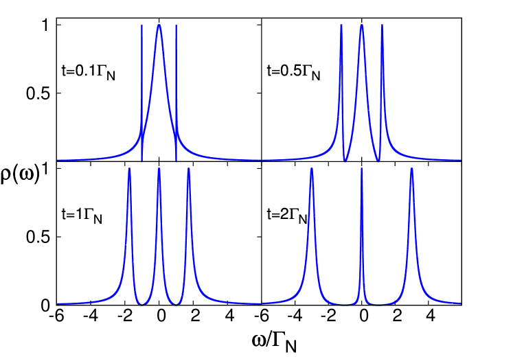
Figure 15: Evolution of the spectral function $\rho(\omega)$ for varying interdot coupling, from the interferometric (small $t$) to the molecular (large $t$) regions.

In this appendix we illustrate how the molecular (i.e. three peak structure of QD₀ spectrum) gradually emerges from the interferometric (weak interdot coupling) scenario, considering both the external electrodes to be metallic trocha2008a ; trocha2008b ; vernek2010 . For simplicity we neglect the correlations and introduce the effective coupling $\Gamma_{N}+\Gamma_{S}\rightarrow\Gamma_{N}$. The selfenergy is diagonal, therefore we can restrict our considerations only to the ‘11’ term

$${{\mbox{\boldmath{$\Sigma$}}}}^{U_{0}=0}_{0,11}(\omega)=-i\frac{\Gamma_{N}}{2}+\frac{t^{2}}{\omega-\epsilon_{+1}}+\frac{t^{2}}{\omega-\epsilon_{-1}}.$$ (19)

Figure 16: Evolution of the spectral function $\rho(\omega)$ with respect to the detuning energy $\delta$ obtained for the uncorrelated case ($U_{j}=0$) in the normal heterostructure ($\Delta=0$).

Figure 15 displays the spectral function $\rho(\omega)$ calculated for several values of $t$. For small values of the interdot coupling, the QD₀ spectrum reveals the asymmetric Fano-type lineshapes fano1961 at $\omega\epsilon_{\pm 1}$. Such structures arise when a dominant (broad) transport channel interferes with a discrete (narrow) state, and can be realized in many areas of physics miroshnichenko2010 . In our case, the Fano resonances originate by combining a ballistic transport through the central QD₀ with additional pathways to/from the adjacent QD_±1. By increasing $t$, the Fano resonances gradually smoothen, and all electronic states nearby the QD_±1 levels $\epsilon_{\pm 1}$ are effectively depleted. In consequence, this induces the three peak (molecular) structure reported in the previous studies vernek2010 . Further increase of the interdot coupling causes a transfer of the spectral weight from the central (subradiant) to the satellite (superradiant) quasiparticle states.

Appearance of the narrow (subradiant) and the broad (superradiant) quasiparticle states can be also induced for a fixed interdot coupling $t$, by reducing the detuning energy $\delta$. This behavior is shown in Fig. 16.

References

- (1) P.A. Orellana, G.A. Lara, and E.V. Anda, Kondo and Dicke effect in quantum dots side coupled to a quantum wire, Phys. Rev. B 74, 193315 (2006).
- (2) R.H. Dicke, The effect of collisions upon the Doppler width of spectral lines, Phys. Rev. 89, 472 (1953).
- (3) T.V. Shahbazyan and M.E. Raikh, Two-channel resonant tunneling, Phys. Rev. B 49, 17123 (1994).
- (4) B. Wunsch and A. Chudnovskiy, Quasistates and their relation to the Dicke effect in a mesoscopic ring coupled to a reservoir, Phys. Rev. B 68, 245317 (2003).
- (5) T. Vorrath and T. Brandes, Dicke effect in the tunnel current through two double quantum dots, Phys. Rev. B 68, 035309 (2003).
- (6) P.A. Orellana, M.L. Ladrón de Guevara, and F. Claro, Controlling Fano and Dicke effects via a magnetic flux in a two-site Anderson model, Phys. Rev. B 70, 233315 (2004).
- (7) T. Brandes, Coherent and collective quantum optical effects in mesoscopic systems, Phys. Rep. 408, 315 (2005).
- (8) M.L. de Guevara and P.A. Orellana, Electronic transport through a parallel-coupled triple quantum dot molecule: Fano resonances and bound states in the continuum, Phys. Rev. B 73, 205303 (2006).
- (9) P. Trocha and J. Barnaś, Dicke-like effect in spin-polarized transport through coupled quantum dots, J. Phys.: Condens. Matt. 20, 125220 (2008).
- (10) P. Trocha and J. Barnaś, Kondo-Dicke resonances in electronic transport through triple quantum dots, Phys. Rev. B 78, 075424 (2008).
- (11) E. Vernek, P.A. Orellana, and S.E. Ulloa, Suppression of Kondo screening by the Dicke effect in multiple quantum dots, Phys. Rev. B 82, 165304 (2010).
- (12) P.P. Baruselli, R. Requist, M. Fabrizio, and E. Tosatti, Ferromagnetic Kondo effect in a triple quantum dot system, Phys. Rev. Lett. 111, 047201 (2013).
- (13) Q. Wang, H. Xie, Y.-H. Nie, and W. Ren, Enhancement of thermoelectric efficiency in triple quantum dots by the Dicke effect, Phys. Rev. B 87, 075102 (2013).
- (14) L. Bai, R. Zhang, and C.-L. Duan, Andreev reflection tunneling through a triangular triple quantum dot system, Physica B 405, 4875 (2010).
- (15) L. Bai, Y.-J. Wu, and B. Wang, Andreev reflection in a triple quantum dot system coupled with a normal-metal and a superconductor, phys. stat. sol. (b) 247, 335 (2010).
- (16) C.-Z. Ye, W.-T. Lu, H. Jiang, and C.-T. Xu, The Andreev tunneling behaviors in the FM/QD/SC system with intradot spin-flip scattering, Physica E 74, 588 (2015).
- (17) W.-P. Xu, Y.-Y. Zhang, Q. Wang, Z.-J. Li, and Y.-H. Nie, Thermoelectric effects in triple quantum dots coupled to a normal and a superconducting leads, Phys. Lett. A 380, 958 (2016).
- (18) G.-Y. Yi, X.-Q. Wang, H.-N. Wu, and W.-J. Gong, Nonlocal magnetic configuration controlling realized in a triple-quantum-dot Josephson junction, Physica E 81, 26 (2016).
- (19) X.-Q. Wang, G.-Y. Yi, and W.-J. Gong, Dicke-Josephson effect in a cross-typed triple-quantum-dot junction, Sol. State Commun. 247, 12 (2016).
- (20) J. Bauer, A. Oguri, & A.C. Hewson, Spectral properties of locally correlated electrons in a Bardeen-Cooper-Schrieffer superconductor, J. Phys.: Condens. Matter 19, 486211 (2007).
- (21) L. Li, Z. Cao, T.-F. Fang, H.-G. Luo, and W.-Q. Chen, Kondo screening of Andreev bound states in a normal-quantum dot-superconductor system, Phys. Rev. B 94, 165144 (2016).
- (22) R.S. Deacon, Y. Tanaka, A. Oiwa, R. Sakano, K. Yoshida, K. Shibata, K. Hirakawa, and S. Tarucha, Tunneling spectroscopy of andreev energy levels in a quantum dot coupled to a superconductor, Phys. Rev. Lett. 104, 076805 (2010).
- (23) E.J.H. Lee, X. Jiang, R. Aguado, G. Katsaros, C.M. Lieber, and S. De Franceschi, Zero-bias anomaly in a nanowire quantum dot coupled to superconductors, Phys. Rev. Lett. 109, 186802 (2012).
- (24) J.-D. Pillet, P. Joyez, R Žitko, and M.F. Goffman, Tunneling spectroscopy of a single quantum dot coupled to a superconductor: from Kondo ridge to Andreev bound states, Phys. Rev. B 88, 045101 (2013).
- (25) R. Žitko, J.S. Lim, R. López, and R. Aguado, Shiba states and zero-bias anomalies in the hybrid normal-superconductor Anderson model, Phys. Rev. B 91, 045441 (2015).
- (26) T. Domański, I. Weymann, M. Barańska, and G. Górski, Constructive influence of the induced electron pairing on the Kondo state, Sci. Rep. 6, 23336 (2016).
- (27) M. Žonda, V. Pokorný, V. Janiš, & T. Novotný, Perturbation theory of a superconducting - impurity quantum phase transition, Sci. Rep. 5, 8821 (2015); T. Domański, M. Žonda, V. Pokorný, G. Górski, V. Janiš, T. Novotný, Josephson-phase-controlled interplay between the correlation effects and electron pairing in a three-terminal nanostructure Phys. Rev. B 95, 045104 (2017).
- (28) H.J.W. Haug and A.-P. Jauho, Quantum kinetics in transport and optics of semiconductors, Springer-Verlag, (Berlin, Heidelberg, New York) (2008).
- (29) K. G. Wilson, The renormalization group: Critical phenomena and the Kondo problem, Rev. Mod. Phys. 47, 773 (1975).
- (30) A.V. Rozhkov and D.P. Arovas, Interacting-impurity Josephson junction: Variational wave functions and slave-boson mean-field theory, Phys. Rev. B 62, 6687 (2000).
- (31) We use open-access Budapest Flexible DM-NRG code, http://www.phy.bme.hu/dmnrg/; O. Legeza, C. P. Moca, A. I. Tóth, I. Weymann, G. Zaránd, Manual for the Flexible DM-NRG code, arXiv:0809.3143 (2008, unpublished).
- (32) F.B. Anders and A. Schiller, Real-Time Dynamics in Quantum-Impurity Systems: A Time-Dependent Numerical Renormalization-Group Approach, Phys. Rev. Lett. 95, 196801 (2005); Spin precession and real-time dynamics in the Kondo model: Time-dependent numerical renormalization-group study, Phys. Rev. B 74, 245113 (2006).
- (33) A. Weichselbaum and J. von Delft, Sum-Rule Conserving Spectral Functions from the Numerical Renormalization Group, Phys. Rev. Lett. 99, 076402 (2007).
- (34) W.C. Oliveira and L.N. Oliveira, Generalized numerical renormalization-group method to calculate the thermodynamical properties of impurities in metals, Phys. Rev. B 49, 11986 (1994).
- (35) F.D.M. Haldane, Scaling Theory of the Asymmetric Anderson Model, Phys. Rev. Lett. 40, 416 (1978).
- (36) U. Fano, Effects of configuration interaction on intensities and phase shifts, Phys. Rev. 124, 1866 (1961).
- (37) A.E. Miroshnichenko, S. Flach, and Y.S. Kivshar, Fano resonances in nanoscale structures, Rev. Mod. Phys. 82, 2257 (2010).