When the Hotter Cools More Quickly: Mpemba Effect in Granular Fluids

Abstract

Under certain conditions, two samples of fluid at different initial temperatures present a counterintuitive behavior known as the Mpemba effect: it is the hotter system that cools sooner. Here, we show that the Mpemba effect is present in granular fluids, both in uniformly heated and in freely cooling systems. In both cases, the system remains homogeneous, and no phase transition is present. Analytical quantitative predictions are given for how differently the system must be initially prepared to observe the Mpemba effect, the theoretical predictions being confirmed by both molecular dynamics and Monte Carlo simulations. Possible implications of our analysis for other systems are also discussed.

Let us consider two identical beakers of water, initially at two different temperatures, put in contact with a thermal reservoir at subzero (on the Celsius scale) temperature. While one may intuitively expect that the initially cooler sample would freeze first, it has been observed that this is not always the case Mpemba and Osborne (1969). This paradoxical behavior named the Mpemba effect (ME) has been known since antiquity and discussed by philosophers like Aristotle, Roger Bacon, Francis Bacon, and Descartes Jeng (2006); Brownridge (2011). Nevertheless, physicists only started to analyze it in the second part of the past century, mainly in popular science or education journals Jeng (2006); Brownridge (2011); Mpemba and Osborne (1969); Kell (1969); Firth (1971); Deeson (1971); Frank (1974); Gallear (1974); Walker (1977); Osborne (1979); Freeman (1979); Kumar (1980); Hanneken (1981); Auerbach (1995); Knight (1996); Courty and Kierlik (2006); Katz (2009); Wang et al. ; Balážovič and Tomášik (2012); Sun (2015); Balážovič and Tomášik (2015); Romanovsky (2015); Ibekwe and Cullerne (2016).

There is no consensus on the underlying physical mechanisms that bring about the ME. Specifically, water evaporation Kell (1969); Firth (1971); Walker (1977); Vynnycky and Mitchell (2010), differences in the gas composition of water Freeman (1979); Wojciechowski et al. (1988); Katz (2009), natural convection Deeson (1971); Maciejewski (1996); Ibekwe and Cullerne (2016), or the influence of supercooling, either alone Auerbach (1995); Zhang et al. (2014) or combined with other causes Esposito et al. (2008); Vynnycky and Maeno (2012); Vynnycky and Kimura (2015); Jin and Goddard (2015), have been claimed to have an impact on the ME. Conversely, the own existence of the ME in water has been recently put in question Burridge and Linden (2016). Notwithstanding, Mpemba-like effects have also been observed in different physical systems, such as carbon nanotube resonators Greaney et al. (2011) or clathrate hydrates Ahn et al. (2016).

The ME requires the evolution equation for the temperature to involve other variables, which may facilitate or hinder the temperature relaxation rate. The initial values of those additional variables depend on the way the system has been prepared, i.e., “aged,” before starting the relaxation process. Typically, aging and memory effects are associated with slowly evolving systems with a complex energy landscape, such as glassy Kovacs et al. (1979); Bouchaud (1992); Prados et al. (1997); Bonilla et al. (1998); Berthier and Bouchaud (2002); Mossa and Sciortino (2004); Aquino et al. (2008); Prados and Brey ; Ruiz-García and Prados (2014) or dense granular systems Nicodemi and Coniglio (1999); Josserand et al. (2000); Brey and Prados (2001). However, these effects have also been observed in simpler systems, like granular gases Ahmad and Puri (2007); Brey et al. (2007); Prados and Trizac (2014); Trizac and Prados (2014) or, very recently, crumpled thin sheets and elastic foams Lahini et al. (2017).

In a general physical system, the study of the ME implies finding those additional variables that control the temperature relaxation and determining how different they have to be initially in order to facilitate its emergence. In order to quantify the effect with the tools of nonequilibrium statistical mechanics, a precise definition thereof is mandatory. An option is to look at the relaxation time to the final temperature as a function of the initial temperature Mpemba and Osborne (1969); Kell (1969); Firth (1971); Freeman (1979); Walker (1977); Jeng (2006); Vynnycky and Mitchell (2010); Burridge and Linden (2016); Ahn et al. (2016). Alternatively, one can analyze the relaxation curves of the temperature: if the curve for the initially hotter system crosses that of the initially cooler one and remains below it for longer times, the ME is present Walker (1977); Esposito et al. (2008); Brownridge (2011); Greaney et al. (2011); Wang et al. ; Vynnycky and Maeno (2012); Zhang et al. (2014); Sun (2015); Vynnycky and Kimura (2015).

In this Letter, we combine both alternatives above and investigate the ME in a prototypical case of intrinsically out-of-equilibrium system: a granular fluid Haff (1983); Goldhirsch (2003); Pöschel and Luding (2001); Aranson and Tsimring (2009), i.e., a (dilute or moderately dense) set of mesoscopic particles that do not preserve energy upon collision. As a consequence, the mean kinetic energy, or granular temperature $T(t)$ Goldhirsch (2003), decays monotonically in time unless an external energy input is applied. The simplicity of the granular fluid makes it an ideal benchmark for other, more complex, nonequilibrium systems. We analyze the time evolution of the granular fluid starting from different initial preparations and quantitatively investigate how the ME appears. This is done for both the homogeneous heated and freely cooling cases.

Our granular fluid is composed of smooth inelastic hard spheres. Therefore, the component of the relative velocity along the line joining the centers of the two colliding particles is reversed and shrunk by a constant factor $\alpha$ Haff (1983), the so-called coefficient of normal restitution. In addition, the particles are assumed to be subject to random forces in the form of a white-noise thermostat with variance $m^{2}\xi^{2}$, where $m$ is the mass of a particle. Thus, the velocity distribution function (VDF) $f(\bm{v},t)$ obeys an Enskog-Fokker-Planck kinetic equation van Noije and Ernst (1998); Montanero and Santos (2000); García de Soria et al. (2012).

The granular temperature and the excess kurtosis (or second Sonine coefficient) are defined as $T(t)=\frac{m}{3}\langle v^{2}(t)\rangle\equiv\frac{m}{3n}\int d\bm{v}\,v^{2}f(\bm{v},t)$ and $a_{2}=\frac{3}{5}\langle v^{4}\rangle/\langle v^{2}\rangle^{2}-1$, respectively, where $n=\int d\bm{v}f(\bm{v},t)$ is the number density. From the kinetic equation for the VDF, one readily finds van Noije and Ernst (1998)

$$\frac{dT}{dt}= -\frac{2\kappa}{3}\left(\mu_{2}T^{3/2}-\chi\right),$$ (1a)

$$\frac{d\ln(1+a_{2})}{dt}= \frac{4\kappa}{3T}\left(\mu_{2}T^{3/2}-\chi-\frac{\frac{1}{5}\mu_{4}T^{3/2}-\chi}{1+a_{2}}\right),$$ (1b)

where $\kappa\equiv 2ng(n)\sigma^{2}\sqrt{\pi/m}$, $\sigma$ and $g(n)$ are the sphere diameter and the pair correlation function at contact Carnahan and Starling (1969), respectively, $\chi\equiv\frac{3m}{2\kappa}\xi^{2}$, and $\mu_{2}$ and $\mu_{4}$ are dimensionless collisional rates.

Note that Eqs. (1) are formally exact, but (a) $T$ and $a_{2}$ are coupled, and (b) the equations are not closed in those two variables since $\mu_{n}$ are functionals of the whole VDF. However, if inelasticity is not too large, the nonlinear contributions of $a_{2}$ and the complete contributions of higher order cumulants can be neglected. This is the so-called first Sonine approximation van Noije and Ernst (1998); Santos and Montanero (2009), which yields $\mu_{n}\simeq\mu_{n}^{(0)}+\mu_{n}^{(1)}a_{2}$, with $\mu_{2}^{(0)}=1-\alpha^{2}$, $\mu_{2}^{(1)}=\frac{3}{16}\mu_{2}^{(0)}$, $\mu_{4}^{(0)}=\left(\frac{9}{2}+\alpha^{2}\right)\mu_{2}^{(0)}$, $\mu_{4}^{(1)}=(1+\alpha)\left[2+\frac{3}{32}(69+10\alpha^{2})(1-\alpha)\right]$.

Using the first Sonine approximation above in Eqs. (1), they become a closed set, but the $T$-$a_{2}$ coupling still remains. Taking into account this coupling, and since $\mu_{2}$ is an increasing function of $a_{2}$, it turns out that the relaxation of the granular temperature $T$ from an initially “cooler” (smaller $T$) sample could possibly be overtaken by that of an initially “hotter” one, if the initial excess kurtosis of the latter is larger enough. We build on and quantify the implications of this physical idea in the following.

First, we consider the uniformly heated case (i.e., $\chi\neq 0$) and prepare the granular fluid in an initial state that is close to the steady one, in the sense that Eqs. (1) can be linearized around the stationary values van Noije and Ernst (1998); Montanero and Santos (2000) $T_{\text{st}}=\left(\chi/\mu_{2}^{{\text{st}}}\right)^{\frac{2}{3}}$ and $a_{2}^{\text{st}}=[5\mu_{2}^{(0)}-\mu_{4}^{(0)}]/[\mu_{4}^{(1)}-5\mu_{2}^{(1)}]$, where $\mu_{n}^{{\text{st}}}=\mu_{n}^{(0)}+\mu_{n}^{(1)}a_{2}^{{\text{st}}}$.

Let us use a dimensionless temperature $\theta=T/T_{{\text{st}}}$ and define $\delta\theta=\theta-1$, $\delta a_{2}=a_{2}-a_{2}^{{\text{st}}}$, and $\tau=\kappa\sqrt{T_{{\text{st}}}}t$. A straightforward calculation gives

$$\frac{d}{d\tau}\begin{pmatrix}\delta\theta\\ \delta a_{2}\end{pmatrix}=-\mathsf{\Lambda}\cdot\begin{pmatrix}\delta\theta\\ \delta a_{2}\end{pmatrix},$$ (2)

where the matrix $\mathsf{\Lambda}$ has elements ${\Lambda}_{11}=\mu_{2}^{{\text{st}}}$, ${\Lambda}_{12}=\frac{2}{3}\mu_{2}^{(1)}$, ${\Lambda}_{21}=-2\mu_{2}^{{\text{st}}}a_{2}^{{\text{st}}}$, and ${\Lambda}_{22}=\frac{4}{15}[\mu_{4}^{(1)}-5\mu_{2}^{(1)}(1+a_{2}^{{\text{st}}})]$. Thus, the relaxation of the temperature reads

$$\delta\theta = \frac{1}{\gamma}\left[(\lambda_{+}-\mu_{2}^{{\text{st}}})\delta\theta_{0}-\frac{2}{3}\mu_{2}^{(1)}\delta a_{2,0}\right]e^{-\lambda_{-}\tau}$$ (3)

$$-\frac{1}{\gamma}\left[(\lambda_{-}-\mu_{2}^{{\text{st}}})\delta\theta_{0}-\frac{2}{3}\mu_{2}^{(1)}\delta a_{2,0}\right]e^{-\lambda_{+}\tau},$$

where $\lambda_{\pm}=\frac{1}{2}\left[\Lambda_{11}+\Lambda_{22}\pm\sqrt{(\Lambda_{11}-\Lambda_{22})^{2}+4\Lambda_{12}\Lambda_{21}}\right]$ are the eigenvalues of the matrix $\mathsf{\Lambda}$ and $\gamma\equiv\lambda_{+}-\lambda_{-}>0$.

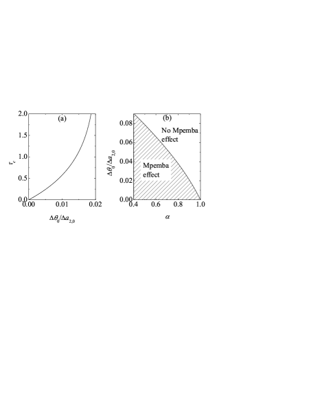
Figure 1: (a) Crossover time $\tau_{c}$ as a function of the ratio $\Delta\theta_{0}/\Delta a_{2,0}$ for $\alpha=0.9$. (b) Phase diagram in the plane $\Delta\theta_{0}/\Delta a_{2,0}$ vs $\alpha$. The regions of the plane inside which there appears or does not appear the ME are separated by the curve $(\Delta\theta_{0}/\Delta a_{2,0})_{\text{max}}$.

Let us imagine two initial states $f_{0}=f_{A}$ and $f_{B}$, with $(\theta_{0},a_{2,0})=(\theta_{A},a_{2A})$ and $(\theta_{B},a_{2B})$, respectively. We assume that $\theta_{A}>\theta_{B}$ and $a_{2A}>a_{2B}$. Both cooling ($\theta_{A}>\theta_{B}>1$) and heating ($\theta_{B}<\theta_{A}<1$) processes may be considered. From Eq. (3), the time $\tau_{c}$ for the possible crossing of the two relaxation curves satisfies

$$\tau_{c}=\frac{1}{\gamma}\ln\frac{2\mu_{2}^{(1)}-3(\lambda_{-}-\mu_{2}^{{\text{st}}})\Delta\theta_{0}/\Delta a_{2,0}}{2\mu_{2}^{(1)}-3(\lambda_{+}-\mu_{2}^{{\text{st}}})\Delta\theta_{0}/\Delta a_{2,0}},$$ (4)

where $\Delta\theta_{0}=\theta_{A}-\theta_{B}$ and $\Delta a_{2,0}=a_{2A}-a_{2B}$. For a given $\alpha$, in this simplified description the crossover time $\tau_{c}$ depends on $(\theta_{A},a_{2A})$ and $(\theta_{B},a_{2B})$ (or, more generally, on the details of the two initial VDFs $f_{A}$ and $f_{B}$) only through the single control parameter $\Delta\theta_{0}/\Delta a_{2,0}$.

Figure 1(a) displays $\tau_{c}$ as a function of the ratio $\Delta\theta_{0}/\Delta a_{2,0}$ for $\alpha=0.9$. Equation (4) implies that there is a maximum of the control parameter $\Delta\theta_{0}/\Delta a_{2,0}$ for which the ME can be observed, namely,

$$\left(\frac{\Delta\theta_{0}}{\Delta a_{2,0}}\right)_{\text{max}}=\frac{2}{3}\frac{\mu_{2}^{(1)}}{\lambda_{+}-\mu_{2}^{{\text{st}}}}.$$ (5)

This quantity determines the phase diagram for the occurrence of the ME, as shown in Fig. 1(b).

Equation (5) can be read in two alternative ways. First, it means that, for a given difference $\Delta a_{2,0}$ of the initial kurtosis, the ME appears when the difference $\Delta\theta_{0}$ of the scaled initial temperatures is below a maximum value $(\Delta\theta_{0})_{\text{max}}$, proportional to $\Delta a_{2,0}$. Second, for a given value of $\Delta\theta_{0}$, the ME is observed only for a large enough difference of the initial kurtosis, i.e., $\Delta a_{2,0}>(\Delta a_{2,0})_{\text{min}}$, with $(\Delta a_{2,0})_{\text{min}}$ proportional to $\Delta\theta_{0}$. This quantitatively measures how different the initial conditions of the system must be in order to have the ME.

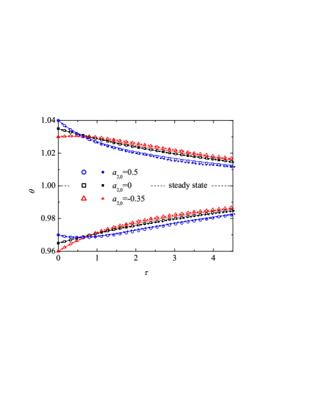
Figure 2: Relaxation of the scaled temperature to the steady state for $\alpha=0.9$. The upper and the lower curves correspond to the ME for the cooling and heating processes, respectively (see text). The direct simulation Monte Carlo (DSMC) (open symbols) and molecular dynamics (MD) (filled symbols) data show an excellent agreement with the theoretical prediction (lines).

In order to check the accuracy of our theoretical results, we compare them in Fig. 2 with MD simulations (at a density $n\sigma^{3}=0.02$) and with the numerical integration of the Enskog-Fokker-Planck equation by means of the DSMC method Bird (1994). In all our simulations, $\alpha=0.9$ and the initial VDF is assumed to have a gamma-distribution form Hogg and Craig (1978) in the variable $v^{2}$ with parameters adjusted to reproduce the chosen values of $\theta_{0}$ and $a_{2,0}$. First, three different initial conditions (A, B, and C) with temperatures above the stationary, $\theta_{A}=1.04$, $\theta_{B}=1.035$, and $\theta_{C}=1.03$, and excess kurtosis $a_{2A}=0.5$, $a_{2B}=0$, and $a_{2C}=-0.35$, are considered. The ME is clearly observed as a crossover of the relaxation curves of the temperature [see, also, Fig. 1(a)]. Second, we analyze a “heating” protocol by choosing initial temperatures below the steady value, namely, $\theta_{A}^{\prime}=0.97$, $\theta_{B}^{\prime}=0.965$, and $\theta_{C}^{\prime}=0.96$, with the same values of the excess kurtosis as in the “cooling” case. Again, a crossover in the temperature relaxation curves appears, signaling the granular analog of the inverse ME proposed in a recent work Lu and Raz (2017). It is interesting to note that the evolution curves corresponding to $\theta_{C}=1.03$ and $\theta_{A}^{\prime}=0.97$ are nonmonotonic. This peculiar behavior is predicted by Eq. (3) to take place if $-\frac{2}{3}\mu_{2}^{(1)}/\mu_{2}^{\text{st}}<\delta\theta_{0}/\delta a_{2,0}<0$.

Figure 3: Relaxation time $\tau_{\epsilon}$ (with $\epsilon=10^{-4}$) as a function of the initial scaled temperature $\theta_{0}$ for $\alpha=0.9$. Three values of the initial excess kurtosis are considered, $a_{2,0}=0.5$ (solid line), $a_{2,0}=0$ (dotted line), and $a_{2,0}=-0.35$ (dashed line). The horizontal (grey) segments join values of initial temperatures that share the same value of the relaxation time and, thus, mark the onset of either the ME ($\theta_{0}>1$) or the inverse ME ($\theta_{0}<1$).

Alternatively, we can characterize the system celerity for cooling (or heating) by defining a relaxation time $\tau_{\epsilon}$ as the time after which $|\theta(\tau_{\epsilon})-1|<\epsilon$, with $\epsilon\ll 1$. From Eq. (3),

$$\tau_{\epsilon}=\frac{1}{\lambda_{-}}\ln\left|\frac{3(\lambda_{+}-\mu_{2}^{{\text{st}}})\delta\theta_{0}-2\mu_{2}^{(1)}\delta a_{2,0}}{3\epsilon\gamma}\right|.$$ (6)

Figure 3 shows $\tau_{\epsilon}$ as a function of the initial temperature $\theta_{0}$ for $\epsilon=10^{-4}$ and the same values of the initial excess kurtosis as considered in Fig. 2. In this diagram, for a given pair of $a_{2,0}$, the range of initial temperatures for which the ME emerges is clearly visualized. Note that this range does not change if the value of the bound $\epsilon$ is changed to $\epsilon^{\prime}$, since the diagram is only shifted vertically by an amount $\frac{1}{\lambda_{-}}\ln(\epsilon/\epsilon^{\prime})$.

A relevant question is whether or not the ME keeps appearing in the zero driving limit. In the undriven case ($\chi=0$), the granular fluid relaxes to the so-called homogeneous cooling state (HCS) Haff (1983), which is the reference state for deriving the granular hydrodynamics Brey et al. (1998). If the linear relaxation picture developed above remained valid in the nonlinear relaxation regime, at least qualitatively, the answer would be negative. Note that the maximum temperature difference $(\Delta T_{0})_{\text{max}}$ would vanish in the limit as $\chi\to 0$ ($T_{{\text{st}}}\propto\chi^{2/3}\to 0$), as a consequence of $(\Delta\theta_{0})_{\text{max}}$ being independent of $\chi$. Interestingly, we show below that this simple scenario does not hold, and the ME is also observed for very small driving: indeed, $(\Delta T_{0})_{\text{max}}$ remains finite in this limit.

For very small driving, there is a wide initial time region inside which the system evolves as if it were cooling freely. Therefore, for the sake of simplicity, we now take $\chi=0$ in the evolution equations (1). While the system freely cools for all times ($\lim_{t\to\infty}T=0$), the excess kurtosis tends to a constant value van Noije and Ernst (1998); Montanero and Santos (2000) $a_{2}^{\text{HCS}}=[5\mu_{2}^{(0)}-\mu_{4}^{(0)}]/[\mu_{4}^{(1)}-\mu_{4}^{(0)}-5\mu_{2}^{(1)}]$. Since there is no natural temperature scale in the free cooling case, we can make use of dimensionless variables by scaling temperature and time with an arbitrary reference value $T_{{\text{ref}}}$, i.e., $T^{*}=T/T_{{\text{ref}}}$ and $t^{*}=\kappa\sqrt{T_{\text{ref}}}t$.

If present at all, we expect the ME to occur for relatively short times, more specifically, before $a_{2}$ has relaxed to its stationary value $a_{2}^{{\text{HCS}}}$. So as to look for a possible crossover of the cooling curves, we linearize the equations around $T^{*}=1$ (by choosing $T_{{\text{ref}}}$ such that the initial temperatures verify $|T_{0}^{*}-1|\ll 1$) and $a_{2}=a_{2}^{{\text{HCS}}}$. Therefrom, the evolution of $T^{*}$ is obtained as

$$\delta T^{*} = \left(\delta T_{0}^{*}+\frac{2}{3}-\frac{2}{3}\frac{\mu_{2}^{(1)}\delta a_{2,0}}{\lambda_{a}-\mu_{2}^{{\text{HCS}}}}\right)e^{-\mu_{2}^{{\text{HCS}}}t^{*}}$$ (7)

$$+\frac{2}{3}\frac{\mu_{2}^{(1)}\delta a_{2,0}}{\lambda_{a}-\mu_{2}^{{\text{HCS}}}}e^{-\lambda_{a}t^{*}}-\frac{2}{3},$$

where $\delta T^{*}=T^{*}-1$, $\delta{a}_{2,0}=a_{2,0}-a_{2}^{{\text{HCS}}}$, and $\lambda_{a}=\frac{4}{15}[\mu_{4}^{(1)}-5\mu_{2}^{(1)}-2\mu_{4}^{(0)}+5\mu_{2}^{(0)}]$. In turn, $a_{2}$ decays exponentially to $a_{2}^{{\text{HCS}}}$ with a characteristic time $\lambda_{a}^{-1}$.

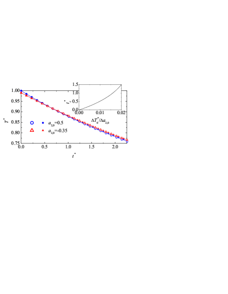
Figure 4: Evolution of the temperature in the free cooling case. Again, the agreement between the theory (lines) and both DSMC (open symbols) and MD (filled symbols) simulation data is excellent. The inset shows $t_{c}^{*}$ as a function of $\Delta T_{0}^{*}/\Delta a_{2,0}$.

Similar to the thermostatted case, we consider two initial states $(T_{0}^{*},a_{2,0})=(T_{A}^{*},a_{2A})$ and $(T_{B}^{*},a_{2B})$, with $\Delta T^{*}_{0}=T_{A}^{*}-T_{B}^{*}>0$, $\Delta a_{2,0}=a_{2A}-a_{2B}>0$. Logically, only the cooling case makes sense. In Fig. 4, we plot two relaxation curves of the temperature for $\alpha=0.9$, with $T_{A}^{*}=1$, $T_{B}^{*}=0.99$, $a_{2A}=0.5$, $a_{2B}=-0.35$, with the choice $T_{{\text{ref}}}=T_{A}$. The ME is clearly observed, and the crossover time $t_{c}^{*}$ is

$$t_{c}^{*}=\frac{1}{\lambda_{a}-\mu_{2}^{{\text{HCS}}}}\ln\left(1-\frac{3}{2}\frac{\lambda_{a}-\mu_{2}^{{\text{HCS}}}}{\mu_{2}^{(1)}}\frac{\Delta T^{*}_{0}}{\Delta a_{2,0}}\right)^{-1};$$ (8)

see inset in Fig. 4. Therefore, there is a maximum value of the ratio $\Delta T^{*}_{0}/\Delta a_{2.0}$ for which the ME appears,

$$\left(\frac{\Delta T^{*}_{0}}{\Delta a_{2,0}}\right)_{\text{max}}=\frac{2}{3}\frac{\mu_{2}^{(1)}}{\lambda_{a}-\mu_{2}^{{\text{HCS}}}}.$$ (9)

Thus, the ME actually survives in the zero driving limit. Had we considered a small value of the driving $\chi$ instead of $\chi=0$, Eqs. (7)–(9) would characterize the strongly nonlinear regime, in which the initial scaled temperature $\theta_{0}=T_{0}/T_{{\text{st}}}\gg 1$. In a first stage of the relaxation, as long as the granular temperature $T\gg T_{s}$, the driving can be neglected, the system freely cools, and the ME is observed provided that the condition (9) is fulfilled. Afterwards, the initially hotter system remains below the initially cooler one forever. When approaching the steady state, both the temperature and the excess kurtosis start to evolve towards their stationary values $T_{\text{st}}$ and $a_{2}^{\text{st}}$, but in both curves one has $a_{2,0}=a_{2}^{{\text{HCS}}}$, and Eq. (5) tells us that no further crossing of the curves takes place ($\Delta a_{2,0}=0$).

In summary, we have shown by means of a simple analytical theory that the ME naturally appears in granular fluids, as a consequence of the relevance of non-Gaussianities in the time evolution of $T$. Specifically, this allows us to (i) prove that the ME is to be expected on quite a general basis and for a wide range of systems, as long as non-Gaussianities are present and (ii) quantitatively predict the region of parameters within which the ME is present. Moreover, we have also predicted the existence of an inverse ME: when the system is heated instead of cooled, the initially cooler sample may heat sooner Lu and Raz (2017). In this way, we have provided a general theoretical framework for the understanding of the ME.

The main assumptions in our theory are: (i) the validity of the kinetic description, (ii) the system remaining homogeneous for all times, and (iii) the first Sonine approximation within the kinetic description. All these assumptions have been validated in the paper. First, the numerical integration of the Enskog equation provided by the DSMC simulations has been successfully compared with MD simulations. Second, we have also checked that the system remains homogeneous in the MD simulations, both for the heated and undriven cases. Concretely, in the latter, the system size has been chosen to be well below the clustering instability threshold Goldhirsch and Zanetti (1993); Aranson and Tsimring (2009). Third, the accuracy of the first Sonine approximation has been confirmed by the excellent agreement between our analytical results and the DSMC simulations, even for the not-so-small values of the excess kurtosis $a_{2}$ considered throughout.

Finally, we stress that non-Gaussianities may have a leading role in the emergence of the ME in other systems, even when there is no inelasticity. For example, the temperature of a molecular fluid, which is basically the mean kinetic energy per particle, does not remain constant if the system interacts with a thermal reservoir. Let us assume that the coupling with the reservoir brings about a nonlinear drag, as considered, for instance, in Refs. Klimontovich (1994); Stout et al. (1995); Fung (1998); Maggi (2013). Then, the evolution equation of the temperature would involve higher moments of the transient nonequilibrium VDF. In this quite general situation, the ME would also stem from those non-Gaussianities Lasanta et al. .