Vertical slice modelling of nonlinear Eady waves using a compatible finite element method

Abstract

A vertical slice model is developed for the Euler-Boussinesq equations with a constant temperature gradient in the direction normal to the slice (the Eady-Boussinesq model). The model is a solution of the full three-dimensional equations with no variation normal to the slice, which is an idealized problem used to study the formation and subsequent evolution of weather fronts. A compatible finite element method is used to discretise the governing equations. To extend the Charney-Phillips grid staggering in the compatible finite element framework, we use the same node locations for buoyancy as the vertical part of velocity and apply a transport scheme for a partially continuous finite element space. For the time discretisation, we solve the semi-implicit equations together with an explicit strong-stability-preserving Runge-Kutta scheme to all of the advection terms. The model reproduces several quasi-periodic lifecycles of fronts despite the presence of strong discontinuities. An asymptotic limit analysis based on the semi-geostrophic theory shows that the model solutions are converging to a solution in cross-front geostrophic balance. The results are consistent with the previous results using finite difference methods, indicating that the compatible finite element method is performing as well as finite difference methods for this test problem. We observe dissipation of kinetic energy of the cross-front velocity in the model due to the lack of resolution at the fronts, even though the energy loss is not likely to account for the large gap on the strength of the fronts between the model result and the semi-geostrophic limit solution.

keywords: mixed finite elements; frontogenesis; Eady model; asymptotic convergence; semi-geostrophic; numerical weather prediction

1 Introduction

In the last two decades, Finite element methods have become a popular discretisation approach for numerical weather prediction (NWP). The main focus has been on spectral elements or discontinuous Galerkin (DG) methods (Fournier et al., 2004; Thomas and Loft, 2005; Dennis et al., 2012; Kelly and Giraldo, 2012; Giraldo et al., 2013; Marras et al., 2013; Brdar et al., 2013; Bao et al., 2015; Marras et al., 2015). Another track of research, which we continue here, has been on compatible finite element methods (e.g. Cotter and Shipton, 2012; Staniforth et al., 2013; Cotter and Thuburn, 2014; McRae and Cotter, 2014; Natale et al., 2016). This work is motivated by the need to move away from the conventional latitude-longitude grids, whilst retaining properties of the Arakawa C-grid staggered finite difference method. The compatible finite element method is a family of mixed finite element methods where different finite element spaces are selected for different variables. Compatible finite element methods are built from finite element spaces that have differential operators such as grad and curl that map from one space to another. This embedded property makes the compatible finite element method analogous to the Arakawa C-grid staggered finite difference method (Arakawa and Lamb, 1977) with extra flexibility in the choice of discretisation to optimize the ratio between global velocity degrees of freedom (DoFs) and global pressure DoFs for the sake of avoiding spurious modes (Cotter and Shipton, 2012). In addition, it allows the use of arbitrary grids with no requirement of orthogonality.

In this study, the compatible finite element method is applied to the Euler-Boussinesq equations with a constant temperature gradient in the $y$-direction: the Eady-Boussinesq vertical slice model (Hoskins and Bretherton, 1972). The model is a solution of the full three-dimensional equations with no variation normal to the slice. As the domain of the vertical slice model consists of a two-dimensional slice, it can be run much quicker on a workstation than a full three-dimensional model. This makes the model ideal for numerical studies and test problems for NWP models. There have been many studies on this idealized problem to examine the formation and subsequent evolution of weather fronts (e.g. Williams, 1967; Nakamura and Held, 1989; Nakamura, 1994; Snyder et al., 1993; Budd et al., 2013; Visram et al., 2014; Visram, 2014). From a mathematical perspective, the connections with optimal transportation have been exposed, leading to new numerical methods and analytical insight (see Cullen (2007) for a review), whilst Cotter and Holm (2013) considered the geometric structure and conservation laws of this slice model. Visram et al. (2014) presented a framework for evaluating model error in terms of asymptotic convergence in the Eady model. The framework is based on the semi-geostrophic (SG) theory in which hydrostatic balance and geostrophic balance of the out-of-slice component of the wind are imposed to the equations. The SG equation provides a suitable limit for asymptotic convergence in the Eady model as the Rossby number decreases to zero (Cullen, 2008). We use this framework to validate the numerical implementation and assess the long term performance of the model developed using the compatible finite element method.

The main goal of this paper is to demonstrate the compatible finite element approach for NWP in the context of this frontogenesis test case. A challenge in using the compatible finite element method in NWP models is the implementation of (the finite element version of) the Charney-Philips grid staggering in the vertical direction that is used in many current operational forecasting models, such as the Met Office Unified Model (Wood et al., 2014). This requires the temperature space to be a tensor product of discontinuous functions in the horizontal direction and continuous functions in the vertical direction (Cotter and Kuzmin, 2016). Therefore we propose a new advection scheme for a partially continuous finite element space and use it to discretise the temperature equation. The other key features of the model are: i) an upwind DG method is applied for the momentum equations; ii) the semi-implicit equations are solved together with an explicit strong-stability-preserving Runge-Kutta (SSPRK) scheme to all of the advection terms; iii) a balanced initialisation is introduced to enforce hydrostatic and geostrophic balances in the initial fields.

The rest of the paper is structured as follows. Section 2 provides the model description, including formation of the Eady problem, discretisation of the governing equations in time and space, and settings of the frontogenesis experiment. In section 3, we present the results of the frontogenesis experiments using the developed model. Here we evaluate model error in terms of SG limit analysis as well as energy dynamics. Finally, in section 4 we provide a summary and outlook.

2 The incompressible Euler-Boussinesq Eady slice model

2.1 Governing equations

In this section, we describe the model equations for the vertical slice Eady problem. The equations are as described in Visram et al. (2014), but we repeat them here to establish notation. To derive a set of equations for the vertical slice Eady problem, we start from the three-dimensional incompressible Euler-Boussinesq equations with rigid-lid conditions on the upper and lower boundaries,

$$\frac{\partial\boldsymbol{u}}{\partial t}+(\boldsymbol{u}\cdot\nabla)\boldsymbol{u}+f\boldsymbol{\hat{z}}\times\boldsymbol{u} = -\frac{1}{\rho_{0}}\nabla p+\frac{g}{\theta_{0}}\theta\boldsymbol{\hat{z}},$$ (1)

$$\frac{\partial\theta}{\partial t}+(\boldsymbol{u}\cdot\nabla)\theta = 0,$$ (2)

$$\nabla\cdot\boldsymbol{u} = 0,$$ (3)

where $\boldsymbol{u}=(u,v,w)$ is the velocity vector, $\nabla=(\partial_{x},\partial_{y},\partial_{z})$ is the gradient operator, and $\boldsymbol{\hat{z}}$ is a unit vector in the $z$-direction; $p$ is the pressure, $\theta$ is the potential temperature, and $g$ is the acceleration due to gravity; $\rho_{0}$ and $\theta_{0}$ are reference density and potential temperature values at the surface, respectively. The rotation frequency $f$ is constant.

In the Eady slice model, we consider perturbations to the constant background temperature and pressure profiles, $\bar{\theta}(y,z)$ and $\bar{p}(y,z)$, respectively. All perturbation variables are then assumed to be independent of $y$, denoted with primed variables as follows,

$$\theta = \bar{\theta}(y,z)+\theta^{\prime}(x,z,t),$$ (4)

$$p = \bar{p}(y,z)+p^{\prime}(x,z,t).$$ (5)

Following Snyder et al. (1993), we select a background profile assuming the geostrophic balance:

$$\bar{\theta}(y,z) = \frac{\theta_{0}}{g}(-f\Lambda y+N^{2}z),$$ (6)

$$-\frac{1}{\rho_{0}}\frac{\partial\bar{p}}{\partial y} = f\Lambda\left(z-\frac{H}{2}\right),$$ (7)

where $\Lambda$ is the constant vertical shear, $N$ is the Brunt-Väisälä frequency, and $H$ is the height of the domain. The variation in $y$ of the background pressure is therefore written as

$$\frac{\partial\bar{p}}{\partial y} = \frac{\rho_{0}g}{\theta_{0}}\frac{\partial\bar{\theta}}{\partial y}\left(z-\frac{H}{2}\right),$$ (8)

where

$$\frac{\partial\bar{\theta}}{\partial y} = -\frac{\theta_{0}f\Lambda}{g}=\mbox{const}.$$ (9)

Similarly, the variation in $z$ of the background pressure is given by the hydrostatic balance as

$$\frac{\partial\bar{p}}{\partial z} = \frac{\rho_{0}g}{\theta_{0}}\bar{\theta}.$$ (10)

Substituting in the background profiles (8) and (10) and $\partial/\partial y=0$ for all perturbation variables, we obtain the nonhydrostatic, incompressible Euler-Boussinesq Eady equations in the vertical slice with rigid-lid conditions on the upper and lower boundaries,

$$\frac{\partial u}{\partial t}+u\frac{\partial u}{\partial x}+w\frac{\partial u}{\partial z}-fv = -\frac{1}{\rho_{0}}\frac{\partial p^{\prime}}{\partial x},$$ (11)

$$\frac{\partial v}{\partial t}+u\frac{\partial v}{\partial x}+w\frac{\partial v}{\partial z}+fu = -\frac{g}{\theta_{0}}\frac{\partial\bar{\theta}}{\partial y}\left(z-\frac{H}{2}\right),$$ (12)

$$\frac{\partial w}{\partial t}+u\frac{\partial w}{\partial x}+w\frac{\partial w}{\partial z} = -\frac{1}{\rho_{0}}\frac{\partial p^{\prime}}{\partial z}+\frac{g}{\theta_{0}}\theta^{\prime},$$ (13)

$$\frac{\partial\theta^{\prime}}{\partial t}+u\frac{\partial\theta^{\prime}}{\partial x}+w\frac{\partial\theta^{\prime}}{\partial z}+v\frac{\partial\bar{\theta}}{\partial y}+w\frac{\partial\bar{\theta}}{\partial z} = 0,$$ (14)

$$\frac{\partial u}{\partial x}+\frac{\partial w}{\partial z} = 0,$$ (15)

where all variables $u,v,w,\theta^{\prime}$ and $p^{\prime}$ are functions of $(x,z,t)$. Now, we redefine the velocity vector and the gradient operator as those in the vertical slice,

$$\boldsymbol{u}=(u,w),\ \ \ \ \nabla=(\partial_{x},\partial_{z}),$$ (16)

and introduce the in-slice buoyancy and the background buoyancy,

$$b^{\prime}=\frac{g}{\theta_{0}}\theta^{\prime},\ \ \ \ \bar{b}=\frac{g}{\theta_{0}}\bar{\theta},$$ (17)

respectively. Finally, dropping the primes gives the vector form of the Eady slice model equations as

$$\frac{\partial\boldsymbol{u}}{\partial t}+(\boldsymbol{u}\cdot\nabla)\boldsymbol{u}-fv\hat{\boldsymbol{x}} = -\frac{1}{\rho_{0}}\nabla p+b\hat{\boldsymbol{z}},$$ (18)

$$\frac{\partial v}{\partial t}+\boldsymbol{u}\cdot\nabla v+f\boldsymbol{u}\cdot\hat{\boldsymbol{x}} = -\frac{\partial\bar{b}}{\partial y}\left(z-\frac{H}{2}\right),$$ (19)

$$\frac{\partial b}{\partial t}+\boldsymbol{u}\cdot\nabla b+\frac{\partial\bar{b}}{\partial y}v+N^{2}\boldsymbol{u}\cdot\hat{\boldsymbol{z}} = 0,$$ (20)

$$\nabla\cdot\boldsymbol{u} = 0,$$ (21)

where $\boldsymbol{\hat{x}}$ is a unit vector in the $x$-direction, and in (20) we used the relationship

$$N^{2}=\frac{g}{\theta_{0}}\frac{\partial\bar{\theta}}{\partial z}=\frac{\partial\bar{b}}{\partial z},$$ (22)

obtained from (6) and (17).

The solutions to the slice model equations (18) to (21) are equivalent to a $y$-independent solution of the full three dimensional equations. The slice model conserves the total energy

$$E=K_{u}+K_{v}+P,$$ (23)

where

$$K_{u} = \rho_{0}\int_{\Omega}\frac{1}{2}|\boldsymbol{u}|^{2}\ \operatorname{d\!}x,$$ (24)

$$K_{v} = \rho_{0}\int_{\Omega}\frac{1}{2}v^{2}\ \operatorname{d\!}x,$$ (25)

$$P = -\rho_{0}\int_{\Omega}b\left(z-\frac{H}{2}\right)\ \operatorname{d\!}x,$$ (26)

are the kinetic energy from the in-slice velocity components, kinetic energy from the out-of-slice velocity component, and potential energy, respectively.

2.2 Finite element discretisation

2.2.1 Compatible finite element spaces

In this study, a compatible finite element method is used to discretise the governing equations. First we take our computational domain, denoted by $\Omega$, to be a rectangle in the vertical plane with a periodic boundary condition in the $x$-direction, and rigid-lid conditions on the upper and lower boundaries. We refer to the combination of the upper and lower boundaries as $\partial\Omega$.

Next we choose finite element spaces with the following properties:

$$\begin{CD}\underbrace{\mathbb{V}_{0}(\Omega)}_{\mbox{\small Continuous}}@>{\nabla^{\perp}}>{}>\underbrace{\mathbb{V}_{1}(\Omega)}_{\mbox{\small Continuous\ normal\ components}}@>{\nabla\cdot}>{}>\underbrace{\mathbb{V}_{2}(\Omega)}_{\mbox{\small Discontinuous}},\end{CD}$$ (27)

where $\nabla^{\perp}=(-\partial_{z},\partial_{x})$, $\mathbb{V}_{0}$ contains scalar-valued continuous functions, $\mathbb{V}_{1}$ contains vector-valued functions with continuous normal components across element boundaries, and $\mathbb{V}_{2}$ contains scalar-valued functions that are discontinuous across element boundaries. The use of these spaces may be considered as an extension of the Arakawa-C horizontal grid staggering in finite difference methods. On quadrilateral elements, Cotter and Shipton (2012) advocated the choice ($\mathbb{V}_{0}$, $\mathbb{V}_{1}$, $\mathbb{V}_{2}$) = (CG_k, RT_k-1, DG_k-1) for $k>0$, where CG_k denotes the continuous finite element space of polynomial degree $k$, RT_k denotes the quadrilateral Raviart-Thomas space of polynomial degree $k$, and DG_k denotes the discontinuous finite element space of polynomial degree $k$. This set of spaces ensures the ratio between global velocity DoFs and global pressure DoFs to be exactly 2:1, which helps to avoid spurious modes. Figure 1 provides diagrams in the vertical plane showing the nodes for the three spaces for the cases $k=1$ and $k=2$.

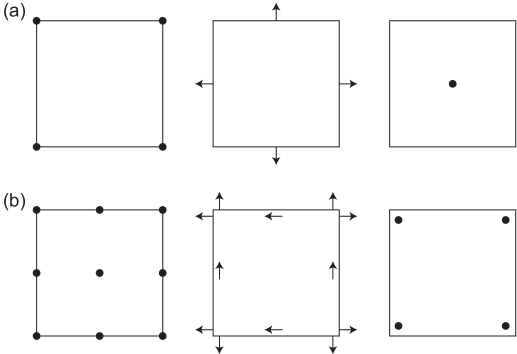
Figure 1: Diagrams showing the nodes for the finite element spaces ($\mathbb{V}_{0}$, $\mathbb{V}_{1}$, $\mathbb{V}_{2}$) = (CG_k, RT_k-1, DG_k-1) on quadrilaterals in the vertical plane. Circles denote scalar nodes, whilst arrows denote normal and tangential components of a vector. Normal components are continuous across element boundaries. Since tangential components are not required to be continuous, these values are not shared by neighbouring elements. (a) From left to right: $\mathbb{V}_{0}$, $\mathbb{V}_{1}$ and $\mathbb{V}_{2}$ with $k$ = 1. (b) From left to right: $\mathbb{V}_{0}$, $\mathbb{V}_{1}$ and $\mathbb{V}_{2}$ with $k$ = 2.

We then restrict the model variables to suitable function spaces. First the velocity and pressure are defined as

$$\quad\boldsymbol{u}\in\mathring{\mathbb{V}}_{1},\quad p\in\mathbb{V}_{2},$$ (28)

where $\mathring{\mathbb{V}}_{1}$ is the subspace defined by

$$\mathring{\mathbb{V}}_{1}=\left\{\boldsymbol{u}\in\mathbb{V}_{1}:\boldsymbol{u}\cdot\boldsymbol{n}=0\mbox{ on }\partial\Omega\right\}.$$ (29)

To be consistent with the three-dimensional Arakawa-C grid staggering, we can choose $v$ from the same space as $p$ as

$$\quad v\in\mathbb{V}_{2}.$$ (30)

There are two main options for arranging the temperature/buoyancy in finite difference models: the Lorenz grid (temperature collocated with pressure), and the Charney-Phillips grid (temperature collocated with vertical velocity). To mimic the Lorenz grid, we can simply choose $b$ from the pressure space $\mathbb{V}_{2}$. In this study, we use the Charney-Phillips grid since it avoids spurious hydrostatic pressure modes. For this purpose, we introduce a scalar space $\mathbb{V}_{b}$ which is obtained by the tensor product of the DG_k-1 space in the horizontal direction and the CG_k space in the vertical direction. As shown in Figure 2, $\mathbb{V}_{b}$ has the same node locations as the vertical part of $\mathbb{V}_{1}$. Then we choose the buoyancy as

$$\quad b\in\mathbb{V}_{b}.$$ (31)

This constructs the extension of the Charney-Phillips staggering to compatible finite element spaces. Natale et al. (2016) showed that this choice of finite element spaces leads to a one-to-one mapping between pressure and buoyancy in the hydrostatic balance equation and therefore, as in the finite difference models using the Charney-Phillips grid, avoids spurious hydrostatic pressure modes. Since the space $\mathbb{V}_{b}$ is discontinuous in the horizontal direction and continuous in the vertical direction, we need a transport scheme for a partially continuous finite element space, which we detail in the next subsection.

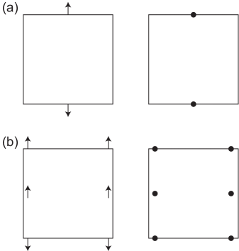
Figure 2: Diagrams showing the nodes for (a) the vertical part of $\mathbb{V}_{1}$ (left) and $\mathbb{V}_{b}$ (right) with $k$ = 1, and (b) those with $k$ = 2. Circles denote scalar nodes, whilst arrows denote normal and tangential components of a vector.

2.2.2 Spatial discretisation

We now use the compatible finite element spaces introduced above to discretise the model equations (18) to (21). Here we start with the discretisation of the in-slice velocity equation (18). First we rewrite the advection term as

$$(\boldsymbol{u}\cdot\nabla)\boldsymbol{u}=(\nabla^{\perp}\cdot\boldsymbol{u})\boldsymbol{u}^{\perp}+\frac{1}{2}\nabla|\boldsymbol{u}|^{2}.$$ (32)

Then, taking (18), dotting with a test function $\boldsymbol{w}\in\mathring{\mathbb{V}}_{1}$, and integrating over the domain gives

$$\int_{\Omega}\boldsymbol{w}\cdot\frac{\partial\boldsymbol{u}}{\partial t}\operatorname{d\!}x+\int_{\Omega}\boldsymbol{w}\cdot(\nabla^{\perp}\cdot\boldsymbol{u})\boldsymbol{u}^{\perp}\operatorname{d\!}x=\int_{\Omega}\boldsymbol{w}\cdot fv\boldsymbol{\hat{x}}\operatorname{d\!}x-\int_{\Omega}\boldsymbol{w}\cdot\nabla\left(\frac{p}{\rho_{0}}+\frac{1}{2}|\boldsymbol{u}|^{2}\right)\operatorname{d\!}x+\int_{\Omega}\boldsymbol{w}\cdot b\hat{\boldsymbol{z}}\operatorname{d\!}x,\ \ \forall\boldsymbol{w}\in\mathring{\mathbb{V}}_{1}.$$ (33)

Recalling that $\boldsymbol{u}$ is in $\mathring{\mathbb{V}}_{1}$, $\nabla^{\perp}\cdot\boldsymbol{u}$ in the second term is not generally defined, since the tangential component of $\boldsymbol{u}$ is not continuous across element boundaries in general. We resolve this by integrating the term by parts. For the contribution to the integral from each element $e$ we obtain

$$\int_{e}\boldsymbol{w}\cdot(\nabla^{\perp}\cdot\boldsymbol{u})\boldsymbol{u}^{\perp}\operatorname{d\!}x=-\int_{e}\nabla^{\perp}(\boldsymbol{w}\cdot\boldsymbol{u}^{\perp})\cdot\boldsymbol{u}\operatorname{d\!}x+\int_{\partial e}\boldsymbol{n}^{\perp}\cdot\tilde{\boldsymbol{u}}\boldsymbol{w}\cdot\boldsymbol{u}^{\perp}\operatorname{d\!}S,$$ (34)

where $\tilde{\boldsymbol{u}}$ is the upwind value of $\boldsymbol{u}$ on the element boundary $\partial e$. Summing over all elements, the advection term becomes

$$\int_{\Omega}\boldsymbol{w}\cdot(\nabla^{\perp}\cdot\boldsymbol{u})\boldsymbol{u}^{\perp}\operatorname{d\!}x=-\int_{\Omega}\nabla^{\perp}(\boldsymbol{w}\cdot\boldsymbol{u}^{\perp})\cdot\boldsymbol{u}\operatorname{d\!}x+\int_{\Gamma}\left[\!\left[\boldsymbol{w}\cdot\boldsymbol{u}^{\perp}\right]\!\right]^{\perp}\cdot\tilde{\boldsymbol{u}}\operatorname{d\!}S,$$ (35)

where $\Gamma$ is the set of interior facets in the finite element mesh with the two sides of each facet arbitrarily labelled by + and −, the jump operator is defined by

$$\left[\!\left[q\right]\!\right] = q^{+}\boldsymbol{n}^{+}+q^{-}\boldsymbol{n}^{-},$$ (36)

$$\left[\!\left[\boldsymbol{v}\right]\!\right] = \boldsymbol{v}^{+}\cdot\boldsymbol{n}^{+}+\boldsymbol{v}^{-}\cdot\boldsymbol{n}^{-},$$ (37)

for any scalar $q$ and vector $\boldsymbol{v}$, and $\tilde{\boldsymbol{u}}$ is evaluated on the upwind side as

$$\tilde{\boldsymbol{u}}=\left\{\begin{array}[]{l}\boldsymbol{u}^{+}\ \ \ \ \mbox{if}\ \boldsymbol{u}\cdot\boldsymbol{n}^{+}<0,\\ \boldsymbol{u}^{-}\ \ \ \ \mbox{otherwise.}\end{array}\right.$$ (40)

A variational derivation and numerical analysis of the discretisation of this term can be found in Natale and Cotter (2016). Turning attention to the pressure gradient term $\nabla\left(\frac{p}{\rho_{0}}+\frac{1}{2}|\boldsymbol{u}|^{2}\right)$, we also integrate by parts. The discrete form of the in-slice velocity equation becomes

$$\int_{\Omega}\boldsymbol{w}\cdot\frac{\partial\boldsymbol{u}}{\partial t}\operatorname{d\!}x = \int_{\Omega}\nabla^{\perp}(\boldsymbol{w}\cdot\boldsymbol{u}^{\perp})\cdot\boldsymbol{u}\operatorname{d\!}x+\int_{\Omega}\nabla\cdot\boldsymbol{w}\left(\frac{p}{\rho_{0}}+\frac{1}{2}|\boldsymbol{u}|^{2}\right)\operatorname{d\!}x$$ (41)

$$+ \int_{\Omega}\boldsymbol{w}\cdot fv\boldsymbol{\hat{x}}\operatorname{d\!}x+\int_{\Omega}\boldsymbol{w}\cdot b\hat{\boldsymbol{z}}\operatorname{d\!}x-\int_{\Gamma}\left[\!\left[\boldsymbol{w}\cdot\boldsymbol{u}^{\perp}\right]\!\right]^{\perp}\cdot\tilde{\boldsymbol{u}}\operatorname{d\!}S,\ \ \forall\boldsymbol{w}\in\mathring{\mathbb{V}}_{1}.$$

The out-of-slice velocity space $\mathbb{V}_{2}$ is discontinuous. An upwind DG treatment of (19) leads to

$$\int_{\Omega}\phi\frac{\partial v}{\partial t}\operatorname{d\!}x-\int_{\Omega}\nabla\cdot(\phi\boldsymbol{u})v\operatorname{d\!}x+\int_{\Gamma}\left[\!\left[\phi\boldsymbol{u}\right]\!\right]\tilde{v}\operatorname{d\!}S+\int_{\Omega}\phi f\boldsymbol{u}\cdot\hat{\boldsymbol{x}}\operatorname{d\!}x+\int_{\Omega}\phi\frac{\partial\bar{b}}{\partial y}\left(z-\frac{H}{2}\right)\operatorname{d\!}x=0,\ \ \forall\phi\in\mathbb{V}_{2},$$ (42)

where $\tilde{v}$ denotes the upwind value of $v$.

We now describe how we discretise the buoyancy equation (20). Recall that $b$ is in the finite element space $\mathbb{V}_{b}$, which is obtained by the tensor product of a discrete finite element space in the horizontal direction with a continuous finite element space in the vertical direction. Therefore we propose a blend of an upwind DG method in the horizontal direction and Streamline Upwind Petrov Galerkin (SUPG) method in the vertical direction. First, multiplying the equation (20) by a test function $\gamma\in\mathbb{V}_{b}$ and integrating it over each column $C$ gives

$$\int_{C}\gamma\frac{\partial b}{\partial t}\operatorname{d\!}x+\int_{C}\gamma\boldsymbol{u}\cdot\nabla b\operatorname{d\!}x+\int_{C}\gamma\frac{\partial\bar{b}}{\partial y}v\operatorname{d\!}x+\int_{C}\gamma N^{2}w\operatorname{d\!}x=0,\ \ \forall\gamma\in\mathbb{V}_{b}.$$ (43)

To obtain the DG formulation, we apply integration by parts in each column,

$$\int_{C}\gamma\frac{\partial b}{\partial t}\operatorname{d\!}x-\int_{C}\nabla\cdot(\gamma\boldsymbol{u})b\operatorname{d\!}x+\int_{C}\gamma\frac{\partial\bar{b}}{\partial y}v\operatorname{d\!}x+\int_{C}\gamma N^{2}w\operatorname{d\!}x+\int_{\partial C}\gamma\boldsymbol{u}\cdot\boldsymbol{n}\tilde{b}\operatorname{d\!}S=0,\ \ \forall\gamma\in\mathbb{V}_{b},$$ (44)

where $\tilde{b}$ denotes the upwind value of $b$ on the column boundary $\partial C$. Integrating by parts again gives

$$\int_{C}\gamma\frac{\partial b}{\partial t}\operatorname{d\!}x+\int_{C}\gamma\boldsymbol{u}\cdot\nabla b\operatorname{d\!}x+\int_{C}\gamma\frac{\partial\bar{b}}{\partial y}v\operatorname{d\!}x+\int_{C}\gamma N^{2}w\operatorname{d\!}x+\int_{\partial C}\gamma\boldsymbol{u}\cdot\boldsymbol{n}\tilde{b}-\gamma\boldsymbol{u}\cdot\boldsymbol{n}b\operatorname{d\!}S=0,\ \ \forall\gamma\in\mathbb{V}_{b},$$ (45)

where the new boundary term contains the value of $b$ on the interior of the column. Summing over the whole domain, we obtain

$$\int_{\Omega}\gamma\frac{\partial b}{\partial t}\operatorname{d\!}x+\int_{\Omega}\gamma\boldsymbol{u}\cdot\nabla b\operatorname{d\!}x+\int_{\Omega}\gamma\frac{\partial\bar{b}}{\partial y}v\operatorname{d\!}x+\int_{\Omega}\gamma N^{2}w\operatorname{d\!}x+\int_{\Gamma_{v}}\left[\!\left[\gamma\boldsymbol{u}\right]\!\right]\tilde{b}-\left[\!\left[\gamma\boldsymbol{u}b\right]\!\right]\operatorname{d\!}S=0,\ \ \forall\gamma\in\mathbb{V}_{b},$$ (46)

where $\Gamma_{v}$ denotes the set of vertical facets of each column. We then apply the SUPG method in the vertical direction by replacing the test function $\gamma$ with $\gamma+\tau\gamma_{z}$, where $\gamma_{z}$ denotes the vertical derivative of $\gamma$:

$$\int_{\Omega}(\gamma+\tau\gamma_{z})\frac{\partial b}{\partial t}\operatorname{d\!}x+\int_{\Omega}(\gamma+\tau\gamma_{z})\boldsymbol{u}\cdot\nabla b\operatorname{d\!}x+\int_{\Omega}\gamma\frac{\partial\bar{b}}{\partial y}v\operatorname{d\!}x+\int_{\Omega}(\gamma+\tau\gamma_{z})N^{2}w\operatorname{d\!}x$$

$$+\int_{\Gamma_{v}}\left[\!\left[(\gamma+\tau\gamma_{z})\boldsymbol{u}\right]\!\right]\tilde{b}-\left[\!\left[(\gamma+\tau\gamma_{z})\boldsymbol{u}b\right]\!\right]\operatorname{d\!}S=0,\ \ \forall\gamma\in\mathbb{V}_{b}.$$ (47)

Here $\tau$ is an upwinding coefficient

$$\tau=c\Delta t\boldsymbol{u}\cdot\hat{\boldsymbol{z}},$$ (48)

where $\Delta t$ is the time step and the constant $c$ is set at $1/15^{\frac{1}{2}}$ following Raymond and Garder (1976).

Finally we discretise the continuity equation (21). Multiplying by a test function $\sigma\in\mathbb{V}_{2}$ and integrating it over the domain $\Omega$ gives

$$\int_{\Omega}\sigma\nabla\cdot\boldsymbol{u}\operatorname{d\!}x=0,\forall\sigma\in\mathbb{V}_{2}.$$ (49)

Since $\nabla\cdot\boldsymbol{u}$ can be defined globally in $\mathbb{V}_{2}$, the projection of (49) is trivial, i.e., the incompressible condition is satisfied exactly under this discretisation.

2.2.3 Time discretisation

Now we discretise the equations (41), (42) and (47) in time using a semi-implicit time-discretisation scheme. This is most easily described as a fixed number of iterations for a Picard iteration scheme applied to a fully implicit time integration scheme.

The implicit time integration scheme is obtained by applying a (possibly off-centred) implicit time discretisation average to all of the forcing terms, as well as the advecting velocity in all of the equations. We then apply an explicit SSPRK scheme to all of the advection terms. To write down the scheme, we first define operators $L_{\boldsymbol{u}}$, $L_{v}$ and $L_{b}$ in the following implicit time-stepping formulation,

$$\int_{\Omega}\boldsymbol{w}\cdot L_{\boldsymbol{u}}\boldsymbol{u}\operatorname{d\!}x = \Delta t\int_{\Omega}\nabla^{\perp}(\boldsymbol{w}\cdot\boldsymbol{u}^{*\perp})\cdot\boldsymbol{u}\operatorname{d\!}x+\Delta t\int_{\Omega}\nabla\cdot\boldsymbol{w}\left(\frac{p^{*}}{\rho_{0}}+\frac{1}{2}|\boldsymbol{u}^{*}|^{2}\right)\operatorname{d\!}x+\Delta t\int_{\Omega}\boldsymbol{w}\cdot fv^{*}\boldsymbol{\hat{x}}\operatorname{d\!}x$$ (50)

$$+ \Delta t\int_{\Omega}\boldsymbol{w}\cdot b^{*}\hat{\boldsymbol{z}}\operatorname{d\!}x-\Delta t\int_{\Gamma}\left[\!\left[\boldsymbol{w}\cdot\boldsymbol{u}^{*\perp}\right]\!\right]^{\perp}\cdot\tilde{\boldsymbol{u}}^{*}\operatorname{d\!}S,\ \ \forall\boldsymbol{w}\in\mathring{\mathbb{V}}_{1},$$

$$\int_{\Omega}\phi L_{v}v\operatorname{d\!}x = \Delta t\int_{\Omega}\nabla\cdot(\phi\boldsymbol{u}^{*})v\operatorname{d\!}x-\Delta t\int_{\Omega}\phi f\boldsymbol{u}^{*}\cdot\hat{\boldsymbol{x}}\operatorname{d\!}x-\Delta t\int_{\Omega}\phi\frac{\partial\bar{b}}{\partial y}\left(z-\frac{H}{2}\right)\operatorname{d\!}x$$ (51)

$$- \Delta t\int_{\Gamma}\left[\!\left[\phi\boldsymbol{u}^{*}\right]\!\right]\tilde{v}^{*}\operatorname{d\!}S,\ \ \forall\phi\in\mathbb{V}_{2},$$

$$\int_{\Omega}(\gamma+\tau\gamma_{z})L_{b}b\operatorname{d\!}x = -\Delta t\int_{\Omega}(\gamma+\tau\gamma_{z})\boldsymbol{u}^{*}\cdot\nabla b\operatorname{d\!}x-\Delta t\int_{\Omega}(\gamma+\tau\gamma_{z})\frac{\partial\bar{b}}{\partial y}v^{*}\operatorname{d\!}x-\Delta t\int_{\Omega}(\gamma+\tau\gamma_{z})N^{2}w^{*}\operatorname{d\!}x$$ (52)

$$- \Delta t\int_{\Gamma_{v}}\left[\!\left[(\gamma+\tau\gamma_{z})\boldsymbol{u}^{*}\right]\!\right]\tilde{b}^{*}-\left[\!\left[(\gamma+\tau\gamma_{z})\boldsymbol{u}^{*}b^{*}\right]\!\right]\operatorname{d\!}S,\ \ \forall\gamma\in\mathbb{V}_{b},$$

where the star denotes $y^{*}=(1-\alpha)y^{n}+\alpha y^{n+1}$ with a time-centring parameter $\alpha$. A 3rd order 3 step SSPRK time-stepping method (Shu and Osher, 1988) is then applied as

$$\varphi^{1}_{y} = y^{n}+L_{y}y^{n},$$ (53)

$$\varphi^{2}_{y} = \frac{3}{4}y^{n}+\frac{1}{4}(\varphi^{1}_{y}+L_{y}\varphi^{1}_{y}),$$ (54)

$$Ay^{n} = \frac{1}{3}y^{n}+\frac{2}{3}(\varphi^{2}_{y}+L_{y}\varphi^{2}_{y}),$$ (55)

for each variable $y=\boldsymbol{u},v$ and $b$, where $A$ is the advection operator.

Finally, we solve for $\boldsymbol{u}^{n+1}$, $v^{n+1}$, $b^{n+1}$ and $p^{n+1}$ iteratively using a Picard iteration method,

$$\int_{\Omega}\boldsymbol{w}\cdot\Delta\boldsymbol{u}\operatorname{d\!}x-\alpha\Delta t\int_{\Omega}\nabla\cdot\boldsymbol{w}\left(\frac{\Delta p}{\rho_{0}}\right)\operatorname{d\!}x-\alpha\Delta t\int_{\Omega}\boldsymbol{w}\cdot f\Delta v\boldsymbol{\hat{x}}\operatorname{d\!}x$$

$$-\alpha\Delta t\int_{\Omega}\boldsymbol{w}\cdot\Delta b\hat{\boldsymbol{z}}\operatorname{d\!}x = -R_{u}[\boldsymbol{w}],\ \ \forall\boldsymbol{w}\in\mathring{\mathbb{V}}_{1},$$ (56)

$$\int_{\Omega}\phi\Delta v\operatorname{d\!}x+\alpha\Delta t\int_{\Omega}\phi f\Delta u\operatorname{d\!}x = -R_{v}[\phi],\ \ \forall\phi\in\mathbb{V}_{2},$$ (57)

$$\int_{\Omega}\gamma\Delta b\operatorname{d\!}x+\alpha\Delta t\int_{\Omega}\gamma N^{2}\Delta w\operatorname{d\!}x = -R_{b}[\gamma],\ \ \forall\gamma\in\mathbb{V}_{b},$$ (58)

$$\int_{\Omega}\sigma\nabla\cdot\Delta\boldsymbol{u}\operatorname{d\!}x = -R_{p}[\sigma],\ \ \forall\sigma\in\mathbb{V}_{2}.$$ (59)

Here $R_{\boldsymbol{u}}[\boldsymbol{w}]$, $R_{v}[\phi]$, $R_{b}[\gamma]$ and $R_{p}[\sigma]$ are the residuals for the implicit system,

$$R_{u}[\boldsymbol{w}] = \int_{\Omega}(\boldsymbol{u}^{n+1}-A\boldsymbol{u}^{n})\cdot\boldsymbol{w}\operatorname{d\!}x,\ \ \forall\boldsymbol{w}\in\mathring{\mathbb{V}}_{1},$$ (60)

$$R_{v}[\phi] = \int_{\Omega}(v^{n+1}-Av^{n})\phi\operatorname{d\!}x,\ \ \forall\phi\in\mathbb{V}_{2},$$ (61)

$$R_{b}[\gamma] = \int_{\Omega}(b^{n+1}-Ab^{n})\gamma\operatorname{d\!}x,\ \ \forall\gamma\in\mathbb{V}_{b},$$ (62)

$$R_{p}[\sigma] = \int_{\Omega}\nabla\cdot\boldsymbol{u}^{n+1}\,\sigma\operatorname{d\!}x,\ \ \forall\sigma\in\mathbb{V}_{2},$$ (63)

where $A$ is as defined in (55). After obtaining $\Delta\boldsymbol{u}$, $\Delta v$, $\Delta b$ and $\Delta p$, we replace $\boldsymbol{u}^{n+1}$, $v^{n+1}$, $b^{n+1}$ and $p^{n+1}$ with $\boldsymbol{u}^{n+1}+\Delta\boldsymbol{u}$ , $v^{n+1}+\Delta v$ , $b^{n+1}+\Delta b$ and $p^{n+1}+\Delta p$, respectively. Then we repeat the iterative procedure for a fixed number of times, which is set to 4 in this study. Figure 3 provides pseudocode for the timestepping procedure. As the 3rd order SSPRK schemes are stable for both DG and SUPG methods, the system is well conditioned for stable Courant numbers, and can be solved with a few iterations of preconditioned GMRES applied to the full coupled system of 4 variables.

$y^{n},\;y^{n+1}\leftarrow y^{0}$ $\triangleright$ initialise

for $k<k_{\mathrm{max}}$ do $\triangleright$ time step loop

     for $i<i_{\mathrm{max}}$ do $\triangleright$ Picard iteration loop

         Compute: $Ay^{n}$ $\triangleright$ advection step using (51)–(53)

         $R_{y}\leftarrow y^{n+1}-Ay^{n}$ $\triangleright$ update residual

         Solve: $J[\Delta y]=-R_{y}$ $\triangleright$ linear solve using (54) – (57)

         $y^{n+1}\leftarrow y^{n+1}+\Delta y$ $\triangleright$ update variables      

     $y^{n}\leftarrow y^{n+1}$ $\triangleright$ advance one time step

Figure 3: Pseudocode for the timestepping procedure. The variable $y$ represents the model variables $\boldsymbol{u},v,b$ and $p$, and $J[\Delta y]$ denotes the Jacobian from the linear system. The constant $i_{\mathrm{max}}$ denotes a fixed number for a Picard iteration, and $k_{\mathrm{max}}$ denotes the total number of time steps.

We use a block diagonal “Riesz-map” preconditioner (Mardal and Winther, 2011) for the GMRES iterations. This operator has an $H(\text{div})$ inner product in the velocity block and mass matrices in the other diagonal blocks; see Natale et al. (2016) for details of $H(\text{div})$ finite element spaces. Inverting the mass matrices is straightforward, requiring only a few iterations of a stationary iteration such as Jacobi; the $H(\text{div})$ block is more challenging due to the non-trivial kernel. We use an LU factorisation, provided by MUMPS – the MUltifrontal Massively Parallel sparse direct Solver (Amestoy et al., 2001, 2006) – to invert it, since we do not currently have access to a suitable preconditioner for this operator.

2.3 Experimental settings

2.3.1 Constants

In the frontogenesis experiments, the model constants are set to the values below, following Nakamura and Held (1989), Cullen (2008), Visram et al. (2014), and Visram (2014):

$$L = 1000\ \mathrm{km},\ H=10\ \mathrm{km},\ f=10^{-4}\ \mathrm{s}^{-1},\$$

$$g = 10\ \mathrm{m\ s}^{-2},\ \rho_{0}=1\ \mathrm{kg\ m}^{-3},\ \theta_{0}=300\ \mathrm{K},$$

$$\Lambda = 10^{-3}\ \mathrm{s}^{-1},\ N^{2}=2.5\times 10^{-5}\ \mathrm{s}^{-1},$$

where $L$ and $H$ determine the model domain $\Omega=[-L,L]\times[0,H]$. The $y$ component of the background buoyancy in (19) and (20) is therefore calculated as

$$\frac{\partial\bar{b}}{\partial y}=-f\Lambda=-10^{-7}\ \mathrm{s}^{-2}.$$ (64)

The Rossby and Froude numbers are given in the model as

$$\mathrm{Ro}=\frac{u_{0}}{fL}=0.05,$$ (65)

$$\mathrm{Fr}=\frac{u_{0}}{NH}=0.1,$$ (66)

where $u_{0}=5\ \mathrm{m\ s}^{-1}$ is a representative velocity. The ratio of Rossby number to the Froude number defines the Burger number,

$$\mathrm{Bu}=\mathrm{Ro}/\mathrm{Fr}=0.5,$$ (67)

which is used when initialising the model.

2.3.2 Initialisation

The model field is initialised with a small perturbation with the wavelength corresponding to the most unstable mode. In this study, the following form of the small perturbation is applied to the in-slice buoyancy,

$$b(x,z) = aN\left\{-\left[1-\frac{\mathrm{Bu}}{2}\coth\left(\frac{\mathrm{Bu}}{2}\right)\right]\sinh Z\cos\left(\frac{\pi x}{L}\right)-n\mathrm{Bu}\cosh Z\sin\left(\frac{\pi x}{L}\right)\right\},$$ (68)

which is the structure of the normal mode taken from Williams (1967). The constant $a$ corresponds to the amplitude of the perturbation, and the constant $n$ takes the form of

$$n=\frac{1}{\mathrm{Bu}}\left\{\left[\frac{\mathrm{Bu}}{2}-\tanh\left(\frac{\mathrm{Bu}}{2}\right)\right]\left[\coth\left(\frac{\mathrm{Bu}}{2}-\frac{\mathrm{Bu}}{2}\right)\right]\right\}^{\frac{1}{2}}.$$ (69)

The modified vertical coordinate $Z$ is defined as

$$Z=\mathrm{Bu}\left[\left(\frac{z}{H}-\frac{1}{2}\right)\right].$$ (70)

Next we initialise the pressure $p$. Given the $b$ in (68), we seek a pressure in hydrostatic balance,

$$\frac{\partial p}{\partial z}=\rho_{0}b.$$ (71)

Since we have rigid-lid conditions at the upper and lower boundaries, we require a symmetry condition for the pressure,

$$\int_{z=0}^{z=H}p(x,z)\operatorname{d\!}z=0,\quad\forall x.$$ (72)

This boundary condition is hard to enforce in the solver, so we first solve for a hydrostatic pressure $\hat{p}$ with a free surface boundary condition on the top,

$$\frac{\partial\hat{p}}{\partial z}-\rho_{0}b=0,\quad\hat{p}(z=H)=0.$$ (73)

The finite element approximation can be found with a test function $\gamma\in\mathbb{V}_{b}$ as

$$\int_{\Omega}\gamma\frac{\partial\hat{p}}{\partial z}\operatorname{d\!}x-\int_{\Omega}\gamma\rho_{0}b\operatorname{d\!}x=-\int_{\Omega}\frac{\partial\gamma}{\partial z}\hat{p}\operatorname{d\!}x-\int_{\Omega}\gamma\rho_{0}b\operatorname{d\!}x=0,\ \ \forall\gamma\in\mathbb{V}_{b},$$ (74)

where we have integrated the pressure gradient term by parts in the second line. We then add an arbitrary function of $x$ to the solution $\hat{p}$ to find $p$ satisfying the symmetry condition (72).

Next we initialize the out-of-slice velocity $v$ by seeking a velocity in geostrophic balance with the initialised $p$ as

$$\frac{\partial p}{\partial x}=\rho_{0}fv.$$ (75)

As $\partial p/\partial x$ is not defined in our finite element framework, first we find $\boldsymbol{s}=\nabla p$ in $\mathring{\mathbb{V}}_{1}$ as

$$\int_{\Omega}\boldsymbol{w}\cdot\boldsymbol{s}\operatorname{d\!}x=\int_{\Omega}\boldsymbol{w}\cdot\nabla p\operatorname{d\!}x=-\int_{\Omega}\nabla\cdot\boldsymbol{w}\,p\operatorname{d\!}x+\int_{\Gamma}\boldsymbol{w}\cdot\boldsymbol{n}p\operatorname{d\!}S,\ \ \forall\boldsymbol{w}\in\mathring{\mathbb{V}}_{1},$$ (76)

where we have integrated the pressure gradient term by parts in the last equality. Then we solve for the initial $v$ as

$$\int_{\Omega}\phi\rho_{0}fv\operatorname{d\!}x=\int_{\Omega}\phi\boldsymbol{s}\cdot\hat{\boldsymbol{x}}\operatorname{d\!}x,\ \ \forall\boldsymbol{\phi}\in\mathbb{V}_{2}.$$ (77)

To initialise the in-slice velocity $\boldsymbol{u}=(u,w)$, we seek a solution to the linear equations for $v$ and $b$,

$$\frac{\partial v_{g}}{\partial t} = -fu-\frac{\partial\bar{b}}{\partial y}\left(z-\frac{H}{2}\right),$$ (78)

$$\frac{\partial b_{g}}{\partial t} = -\frac{\partial\bar{b}}{\partial y}{v_{g}}-N^{2}w,$$ (79)

where we make the SG approximation that $v_{g}$ and $b_{g}$ are given by the geostrophic and hydrostatic balance. If the pressure is in geostrophic and hydrostatic balance then we have

$$\nabla p=\rho_{0}\begin{pmatrix}fv_{g}\\ b_{g}\\ \end{pmatrix},$$ (80)

and therefore we have

$$\nabla\dot{p}=\rho_{0}\begin{pmatrix}f\dot{v}_{g}\\ \dot{b}_{g}\\ \end{pmatrix}=\rho_{0}\begin{pmatrix}-f^{2}u-f\frac{\partial\bar{b}}{\partial y}\left(z-\frac{H}{2}\right)\\ -\frac{\partial\bar{b}}{\partial y}{v_{g}}-N^{2}w\\ \end{pmatrix},$$ (81)

where the dot denotes $\dot{y}=\frac{\partial y}{\partial t}$. We rewrite this in a vector form as

$$\rho_{0}\begin{pmatrix}f^{2}&0\\ 0&N^{2}\\ \end{pmatrix}\boldsymbol{u}+\nabla\dot{p}=\rho_{0}\frac{\partial\bar{b}}{\partial y}\begin{pmatrix}-f\left(z-\frac{H}{2}\right)\\ -{v_{g}}\\ \end{pmatrix}.$$ (82)

The finite element approximation is then

$$\int_{\Omega}\boldsymbol{w}\cdot\rho_{0}\begin{pmatrix}f^{2}&0\\ 0&N^{2}\\ \end{pmatrix}\boldsymbol{u}\operatorname{d\!}x-\int_{\Omega}\nabla\cdot\boldsymbol{w}\dot{p}\operatorname{d\!}x=\int_{\Omega}\boldsymbol{w}\cdot\rho_{0}\frac{\partial\bar{b}}{\partial y}\begin{pmatrix}-f\left(z-\frac{H}{2}\right)\\ -{v_{g}}\\ \end{pmatrix}\operatorname{d\!}x,\quad\forall\boldsymbol{w}\in\mathring{\mathbb{V}}_{1},$$ (83)

where we have integrated the pressure gradient term by parts in the first line. Here we introduce $\psi\in\mathbb{V}_{0}$, with $\nabla^{\perp}\psi=\boldsymbol{u}$, and choose $\boldsymbol{w}=\nabla^{\perp}\xi$, then we have

$$\int_{\Omega}\nabla\xi\cdot\begin{pmatrix}N^{2}&0\\ 0&f^{2}\\ \end{pmatrix}\nabla\psi\operatorname{d\!}x=\int_{\Omega}\nabla\xi\cdot\frac{\partial\bar{b}}{\partial y}\begin{pmatrix}-{v_{g}}\\ f\left(z-\frac{H}{2}\right)\\ \end{pmatrix}\operatorname{d\!}x,\quad\forall\xi\in\mathbb{V}_{0}.$$ (84)

With boundary conditions $\psi=0$ on top and bottom, and substituting the initialised $v$ from (77) for $v_{g}$, we obtain the balanced $\psi$. We then solve for the initial $\boldsymbol{u}$ from $\psi$ to complete the initialisation of the model field.

Finally, we introduce a breeding procedure used by Visram et al. (2014) and Visram (2014) to remove any remaining unbalanced modes in the initial condition. In the experiments performed in section 3, the model field is initialised with a small perturbation by choosing $a$ = -7.5 in (68). The simulation is then advanced for three computational days until the maximum amplitude of $v$ reaches 3 m s^-1, at which point the time is reset to zero to match the amplitude of the initial perturbation with that of Nakamura and Held (1989) and Visram et al. (2014) as closely as possible.

2.3.3 Asymptotic limit analysis

To validate the numerical implementation and assess the long term performance of the model, we introduce the asymptotic limit analysis based on the SG theory. The test outlined here follows that described in Cullen (2008), and used in Visram et al. (2014) and Visram (2014).

First we apply the SG approximation to the governing equations (18) to (21) by imposing the hydrostatic balance and the geostrophic balance of the $v$ component of the wind,

$$-fv\hat{\boldsymbol{x}} = -\frac{1}{\rho_{0}}\nabla p+b\hat{\boldsymbol{z}}.$$ (85)

The equation (85), together with the equations (19) to (21), are the SG equations of the Eady slice model. Now, the solutions of the SG equations are invariant to the changes of variables,

$$x\rightarrow\beta x,\ \ u\rightarrow\beta u,\ \ f\rightarrow\frac{f}{\beta},$$ (86)

where $\beta$ is a rescaling parameter and all other variables are invariant. Recalling the definition of the Rossby number (65), the rescaling (86) converts $\mathrm{Ro}\rightarrow\beta\mathrm{Ro}$. The SG solution therefore provides an asymptotic limit of the model as the Rossby number tends to zero.

With the rescaling parameter $\beta$, the limit of $\mathrm{Ro}\rightarrow 0$ is equivalent to $\beta\rightarrow 0$. Thus the convergence of the model to the SG solution can be tested by performing a sequence of simulations with decreasing $\beta$. Here we follow Cullen (2008) in defining the out-of-slice geostrophic imbalance as

$$\eta=v-\frac{1}{\rho_{0}f}\frac{\partial p}{\partial x},$$ (87)

which is expected to converge at a rate proportional to $\mathrm{Ro}^{2}$, i.e. $\beta^{2}$. To calculate $\eta$ in our finite element framework, first we find the vector of geostrophic and hydrostatic imbalance $\boldsymbol{q}$ in $\mathring{\mathbb{V}}_{1}$ defined as

$$\boldsymbol{q}=\rho_{0}\begin{pmatrix}fv\\ b\\ \end{pmatrix}-\nabla p.$$ (88)

where

$$\eta=\frac{1}{\rho_{0}f}\boldsymbol{q}\cdot\boldsymbol{x}.$$ (89)

The finite element approximation is obtained as

$$\int_{\Omega}\boldsymbol{w}\cdot\boldsymbol{q}\operatorname{d\!}x=\int_{\Omega}\boldsymbol{w}\cdot\rho_{0}\begin{pmatrix}fv\\ b\\ \end{pmatrix}\operatorname{d\!}x-\int_{\Omega}\boldsymbol{w}\cdot\nabla p\operatorname{d\!}x=\int_{\Omega}\boldsymbol{w}\cdot\rho_{0}\begin{pmatrix}fv\\ b\\ \end{pmatrix}\operatorname{d\!}x+\int_{\Omega}\nabla\cdot\boldsymbol{w}\,p\operatorname{d\!}x,\ \ \forall\boldsymbol{w}\in\mathring{\mathbb{V}}_{1},$$ (90)

where we have integrated the pressure gradient term by parts in the third line. We then calculate $\eta$ from $\boldsymbol{q}$ using (89) and assemble it over the domain. If the geostrophic imbalance in the model tends to zero with decreasing $\beta$, then the limit is a solution of the SG equations. This analysis is performed in section 3.2.

3 Results

In this section, we present the results of the frontogenesis experiments using the Eady vertical slice model developed in this study, with the use of the finite element code generation library Firedrake (Rathgeber et al., 2016). The constants used to set up the experiments are shown in section 2.3.1. At the beginning of each experiment, the model is initialised in the way described in section 2.3.2, then integrated for 25 days in each experiment.

The model resolution is given by

$$\Delta x=\frac{2L}{N_{x}},\ \Delta z=\frac{H}{N_{z}},$$ (91)

where $N_{x}$ and $N_{z}$ are the number of quadrilateral elements in the $x$- and $z$-directions, respectively. Unless stated otherwise, we use a resolution of $N_{x}$ = 60 and $N_{z}$ = 30, which is comparable in terms of DoFs to that used in previous work of Visram et al. (2014) and Visram (2014) : $N_{x}$ = 121 and $N_{z}$ = 61. Note that in our model the effective grid spacings are half the size of the lengths given by (91) as we used a higher-order finite element spaces with $k$ = 2, as shown in Figure 1b and Figure 2b, for all experiments. Nakamura and Held (1989) used a lower resolution of $N_{x}$ = 100 and $N_{z}$ = 20. They repeated the experiment with twice the horizontal and vertical resolution (results not shown) and found very small differences to the low-resolution results. Therefore we use their result with $N_{x}$ = 100 and $N_{z}$ = 20 as a comparable result to our control-run result in this section.

For the control run, the time-centring parameter $\alpha$ and the rescaling parameter $\beta$ are set to 0.5 and 1, respectively, and a time step of $\Delta t$ = 50 s is used based on stability requirements. In section 3.1, we investigate the general results of frontogenesis from the control run. Then the asymptotic convergence of the model to the SG limit is examined in section 3.2, by repeating the experiment with various $\beta$. We also assess the effect of off-centring on the long term performance of the model by increasing $\alpha$. Finally, we discuss the model results in terms of energy dynamics in section 3.3.

3.1 General results of frontogenesis

Figures 4(a) and 4(b) show the snapshots of the out-of-slice velocity $v$ and buoyancy $b$ fields, respectively, of the control run. At day 2, both fields show very similar structures to those from the simulation using the linearised equations in Visram (2014). It suggests that at this early stage the motion is well described by the linearised equations.

The model shows some early signs of front formation at day 4. The general shape of the $v$-field is similar to that of day 2. However, the gradient in the cyclonic region is now larger than that in the anticyclonic region, which indicates the beginning of front formation. The maximum gradient in the $v$-field is found at the upper and lower boundaries. In the $b$-field, the region of warm air occupies a smaller area at the lower boundary than it does at the upper boundary. As in the case with $v$, the $b$-field shows the largest gradients near the upper and lower boundaries.

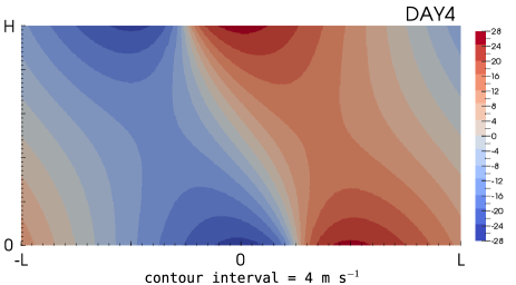
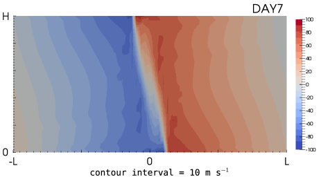
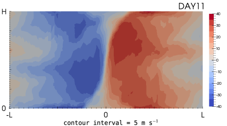
(a) Out-of-slice velocity field. The contour intervals are as specified in each panel.

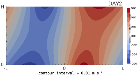
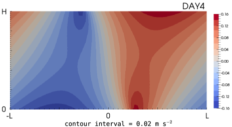
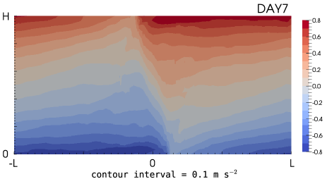
(b) In-slice buoyancy field. The contour intervals are as specified in each panel.

Figure 4: Snapshots of out-of-slice velocity and in-slice bouyancy in the control run at days 2, 4, 7, and 11.

The frontal discontinuity becomes most intense around day 7. Strong gradients are found in both $v$ and $b$ fields. The frontal zone tilts westward with height in both fields. In the $b$-field, the warm region is now lifted off the surface, showing that the front is occluded.

Day 11 corresponds to the first minimum after the initial frontogenesis. At this stage the vertical tilt in the $v$-field reverses, which is a sign of energy conversion from kinetic back to potential energy. In the $b$-field, the discontinuity vanishes and the solution looks almost vertically stratified.

Overall, these results are qualitatively consistent with the early studies (e.g. Williams, 1967; Nakamura and Held, 1989; Nakamura, 1994; Cullen, 2007; Budd et al., 2013; Visram et al., 2014; Visram, 2014). Now, as the out-of-slice velocity is the dominant source of the kinetic energy in the Eady problem, we take it as a quantity to compare the strength of the fronts reproduced in the models.

The thin solid curve in Figure 5 shows the time evolution of the root mean square of $v$ (RMSV) in our model. The result shows that the model reproduces several further quasi-periodic lifecycles after the first frontogenesis. Also shown in Figure 5 in black are the nonlinear results of Nakamura and Held (1989) and Visram et al. (2014), the linear result of Visram (2014), and the SG limit solution from Cullen (2007). All results show a good agreement up to around day 5, where the RMSV of the nonlinear results grow exponentially following the growth of the linear mode. After day 5, at which point the front is close to the grid scale, the nonlinear effects become significant and begin to reduce the growth rate.

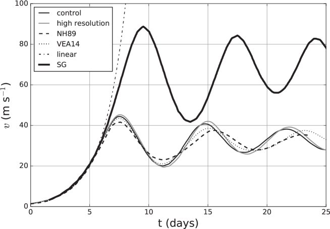
Figure 5: Comparison of the root mean square of the out-of-slice velocity in Eady models. Thin dark solid line shows the result from the control run of this study. Gray line shows the result using two times higher resolution than that of the control run. Dashed and dotted lines show the nonlinear results of Nakamura and Held (1989) and Visram et al. (2014), respectively, and the thick line shows the semi-geostrophic limit solution given by Cullen (2007), based on data from Figure 4 of Visram et al. (2014). Dot-dashed line shows the linear result of Visram (2014) based on data from Figure 5.2a of Visram (2014).

For the period of the first frontogenesis, our result is reasonably close to the result of Visram et al. (2014), who applied a finite difference method with semi-implicit time-stepping and semi-Lagrangian transport on the same governing equations as in this study. Then the two solutions diverge for the subsequent lifecycles. Compared to the result of Nakamura and Held (1989), who used hydrostatic primitive equations with a viscous Eulerian method, both our result and the result of Visram et al. (2014) show larger peak amplitudes of the fronts. However, compared to the SG limit solution given by Cullen (2007), our result, and the results of Nakamura and Held (1989) and Visram et al. (2014), are all much smaller in amplitude. We believe this to be because Cullen (2007) used a Lagrangian discretisation that resolves fronts even at very coarse resolution, and very fine resolution of the front is required to allow this additional transfer of potential to balanced kinetic energy. Visram et al. (2014) showed that the Lagrangian conservation properties were badly violated in the Eulerian calculations, even at higher resolution, concluding that Cullen (2007) is capturing the correct solution after the front is formed.

To evaluate the effect of resolution on our model result, we repeated the experiment using two times higher resolution than that of the control run: ($N_{x}$, $N_{z}$) = (120, 60). A time step of $\Delta t$ = 25 s is used for the high-resolution run. The evolution of RMSV in the high-resolution run is shown by the gray curve in Figure 5. Only a slight increase in the peak amplitudes of RMSV is found in the high-resolution run compared to that of the control run. It indicates that, due to the rapid formation of the frontal discontinuity, the front reaches the grid scale very quickly even when double the resolution is used. As a result, the use of the high resolution can only slightly delay the collapse of the fronts, and thus makes very little contribution to filling the gap between the RMSV values of the model and the SG limit. This result suggests that we would need resolution of several orders of magnitude greater than presently used to reach the RMSV of the SG limit.

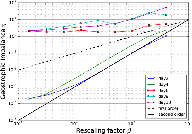
(a) $\alpha=0.5$

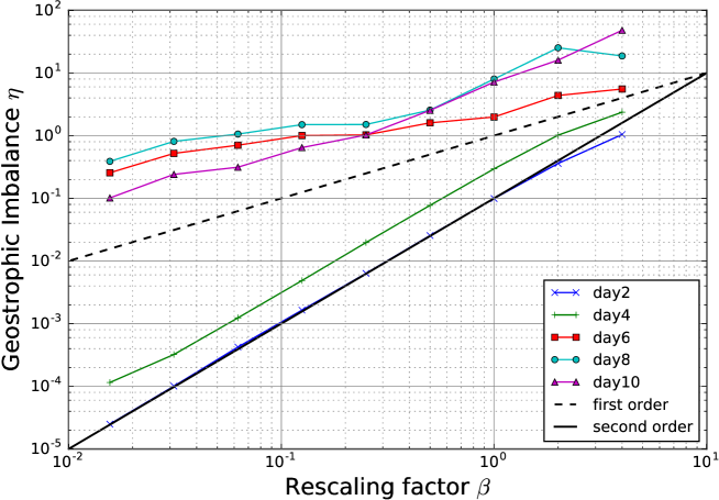
(b) $\alpha=0.55$

Figure 6: Comparison of the geostrophic imbalance in the results of the rescaling tests using (a) $\alpha$ = 0.5, and (b) $\alpha$ = 0.55. Black dashed and solid lines correspond to the first- and second-order convergence rates, respectively. Colored lines show the variations of the geostrophic imbalance with rescaling parameter $\beta$ at day 2, 4, 6, 8 and 10.

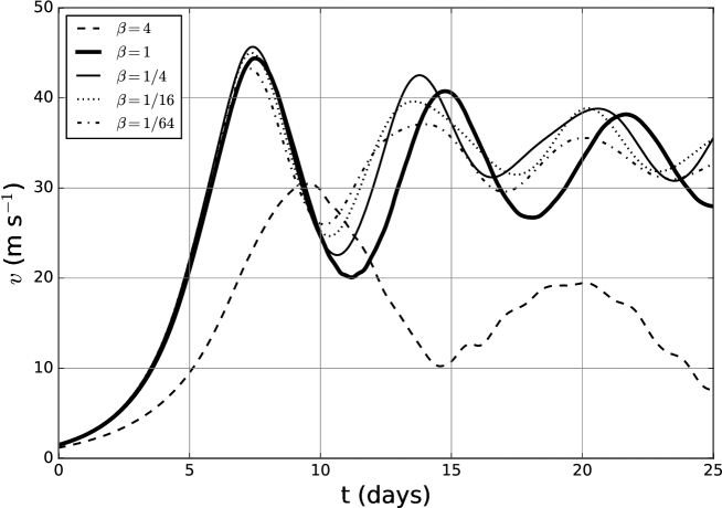
(a) $\alpha=0.5$

(b) $\alpha=0.55$

Figure 7: Comparison of the root mean square of the out-of-slice velocity in the results of the rescaling tests using (a) $\alpha$ = 0.5, and (b) $\alpha$ = 0.55. Thick lines show the results with $\beta$ = 1. The other lines show the results with different values of $\beta$ as shown in the legend.

3.2 Asymptotic convergence to the SG solution

In this section, the validation test of the asymptotic convergence outlined in section 2.3.3 is performed. First, the frontogenesis experiment is repeated using eight different values of the rescaling parameter: $\beta$ = 2², 2, 2^-1, 2^-2, 2^-3, 2^-4, 2^-5, and 2^-6. The time step $\Delta t$ is set to 50 s for the experiments using 2^-2 $\leq$ $\beta$ $\leq$ 2², 25 s for $\beta$ = 2^-3 and 2^-4, and 12.5 s for $\beta$ = 2^-5 and 2^-6. The other settings are the same as the control run. We calculated the geostrophic imbalance $\eta$ defined by (87) in each experiment. We then plotted it over the period of the initial frontogenesis, together with $\eta$ in the control run where $\beta$ is unity.

Figure 6(a) shows the variation of the geostrophic imbalance $\eta$ with rescaling parameter $\beta$ alongside the theoretical first- and second-order convergence rates. The convergence rate starts at around the second-order for $\beta\geq 2^{-3}$ and the first-order for $\beta<2^{-3}$ as shown by the slope at day 2. It improves to the second-order for $\beta\geq 2^{-5}$ at day 4. However, it doesn’t converge at all at day 6, at which point a strong discontinuity is formed in the model. After the peak of the initial frontogenesis at around day 7, the convergence rate recovers a little but stays at less than first-order at days 8 and 10.

For the results in Figure 6(a), the time-centring parameter $\alpha$ is set to 0.5 as that is in the control run. To test the effect of off-centring, the rescaling test was repeated using $\alpha$ = 0.55. This result is shown in Figure 6(b). It shows that increasing the implicitness of the solution gives more balanced solutions. In particular, a reduction of the imbalance is found throughout the initial frontogenesis for $\beta<2^{-3}$. As a result, the overall second-order convergence is achieved at day 2, and the first-order convergence is recovered at day 10 in Figure 6(b). This result is comparable to the result of Visram et al. (2014) (see their Figure 2), where $\alpha=$ 0.55 was used, indicating that the compatible finite element method is performing as well as a finite difference method for this test problem. Note that Visram et al. (2014) used the range of $2^{-3}\leq\beta\leq 2^{2}$, whereas we show the convergence of geostrophic imbalance for smaller $\beta$ as well. The result is also consistent with the results reported by Cullen (2007) with compressible equations.

Figure 7(a) and 7(b) show the evolutions of RMSV in each experiment corresponding to Figure 6(a) and 6(b), respectively. In Figure 7(b), there are some increase in the peak amplitude of fronts compared to that in Figure 7(a), especially in the second peak of the results for $\beta\leq 2^{-2}$. It indicates that damping out some of the unbalanced motion with off-centring improves the predictability of quasi-periodic lifecycles. Compared to the off-centred results of Visram et al. (2014) (see their Figure 4), which very quickly began to diverge as they decreased the Rossby number, our model shows good predictability throughout the range of $\beta$. However, in both cases of Figure 7, decreasing $\beta$ does not make a big difference in the peak amplitude of fronts, thereby leaving the large gap between the model result and the SG limit solution on the strength of the fronts regardless of the value of $\beta$.

3.3 Energy dynamics

In sections 3.1 and 3.2, we showed that our model reproduced results which are consistent with the early model studies based on finite difference methods, and showed that the model solutions converge to a solution in geostrophic balance when we decrease the Rossby number. In this section, we will again look into our result of the control run with focus on the energy dynamics.

Figure 8 shows the time evolution of the total energy $E$, the kinetic energy $K_{u}$ and $K_{v}$, and the potential energy $P$, which are defined by the equations (23) to (26). The kinetic energy $K_{v}$ reaches the maximum amplitude at around day 7, then reduces to the first minimum at around day 11 followed by smaller amplitude lifecycles, just as RMSV does in Figure 5. The time evolution of potential energy $P$ shows the same behaviour with opposite sign, which demonstrates the exchange from potential to kinetic energy over several lifecycles. The amplitude of the kinetic energy $K_{u}$ is very small compared to that of $K_{v}$ and $P$ throughout the experiment. As a result, the total energy $E$ can be interpreted as the difference of the amplitude of $K_{v}$ from that of $P$, which shows a gradual decrease with time.

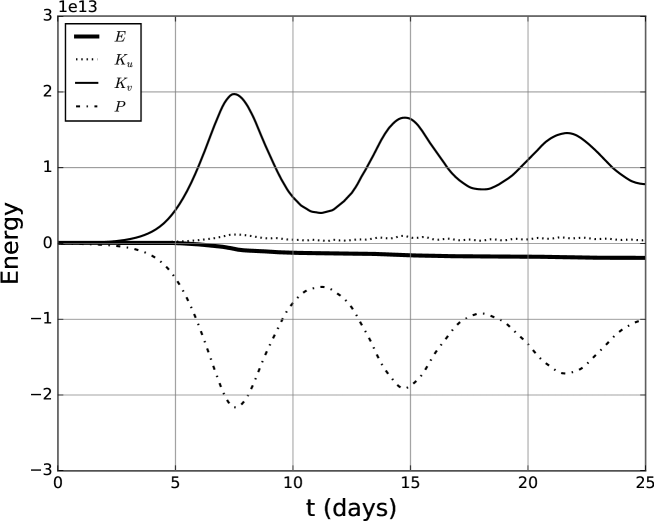
Figure 8: Time evolution of energy of the control run. Thick line represents the evolution of total energy. Dotted and solid lines represent the evolutions of in-slice and out-of-slice components of the kinetic energy. Dot-dashed line represents the evolution of potential energy.

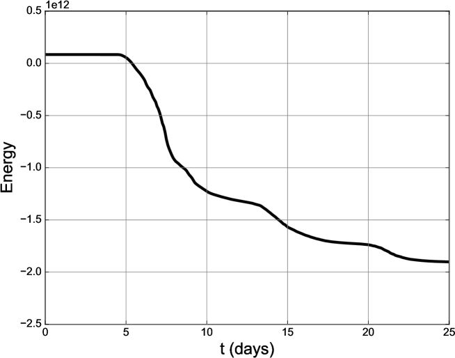
Figure 9: Enlarged view of the evolution of total energy shown in Figure 8. The vertical scale is one order of magnitude less than that of Figure 8.

Figure 9 provides an enlarged view of the time evolution of the total energy. Note that the thick lines in Figure 8 and Figure 9 show the same evolution of the total energy of the control run, and the vertical scale of Figure 9 is one order of magnitude less than that of Figure 8. The total energy stays constant up until day 5, then starts decreasing. It becomes quasi-constant from around day 10 to day 13, then decreases again. By comparing this with the lifecycles of fronts shown as the evolution of RMSV in Figure 5, it appears that the model starts losing energy every time the discontinuity reaches the grid scale. In addition, the reduction in the total energy starts at almost the same time as the RMSV of the control run diverges from the SG solution. Therefore we consider that the lack of resolution is a significant cause of the loss of energy, and it also stops the growth of RMSV too early.

Now, to estimate the potential loss in the kinetic energy $K_{v}$ caused by our advection scheme for $v$, we perform a test considering the dummy velocity $v_{d}$ which obeys the following advection-only equation,

$$\frac{\partial v_{d}}{\partial t}+\boldsymbol{u}\cdot\nabla v_{d} = 0,$$ (92)

and the dummy kinetic energy $K_{v_{d}}$ defined by

$$K_{v_{d}} = \rho_{0}\int_{\Omega}\frac{1}{2}v_{d}^{2}\ \operatorname{d\!}x.$$ (93)

In this test, we solve the equation (92) in parallel with the governing equations (18) to (21). The same experimental settings including the constants, initial and boundary conditions and the resolution as in the control run are used in this test. Here we apply the same advection scheme used for $v$ to $v_{d}$ as

$$\int_{\Omega}\phi\frac{\partial v_{d}}{\partial t}\operatorname{d\!}x-\int_{\Omega}\nabla\cdot(\phi\boldsymbol{u})v_{d}\operatorname{d\!}x+\int_{\Gamma}\left[\!\left[\phi\boldsymbol{u}\right]\!\right]\tilde{v_{d}}\operatorname{d\!}S=0,\ \ \forall\phi\in\mathbb{V}_{2},$$ (94)

and the same semi-implicit time-stepping method described in section 2.2.3 to (94). After every time step, we calculate the difference between $K_{v}$ and $K_{v_{d}}$ as

$$\epsilon=\rho_{0}\int_{\Omega}\frac{1}{2}\{(v_{d}^{n+1})^{2}-(v^{n})^{2}\}\ \operatorname{d\!}x.$$ (95)

Then we replace $v_{d}^{n+1}$ with $v^{n+1}$ and repeat the time integration. By accumulating the energy difference $\epsilon$ every time step, we can estimate the potential loss of kinetic energy caused by the discretisation of the advection term in the $v$ equation (19). This result is shown by the dashed line in Figure 10. Also shown in Figure 10 as the thick line is the loss of total energy in the control run from the initial state. The two energy values are almost identical to each other, showing that almost all the energy loss in the model is caused in the $v$ advection.

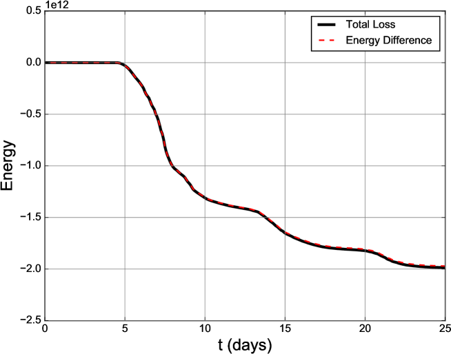
Figure 10: Result of the energy analysis using the dummy velocity. Thick line represents the loss of total energy from the initial state of the control run. Dashed line shows the accumulated difference between the kinetic energy $K_{v}$ and the dummy kinetic energy $K_{v_{d}}$.

To investigate the cause of the energy loss in the $v$ advection, we calculated the residual in the out-of-slice velocity field, which is defined as the difference between LHS and RHS of the equation (19),

$$r_{v}=\frac{\partial v}{\partial t}+\boldsymbol{u}\cdot\nabla v+f\boldsymbol{u}\cdot\hat{\boldsymbol{x}}+\frac{\partial\bar{b}}{\partial y}\left(z-\frac{H}{2}\right).$$ (96)

With $\phi\in\mathbb{V}_{2}$, we calculated $r_{v}$ by solving

$$\int_{\Omega}\phi r_{v}^{n+1}\operatorname{d\!}x=\int_{\Omega}\phi\frac{v^{n+1}-v^{n}}{\Delta t}\operatorname{d\!}x+\int_{\Omega}\phi\boldsymbol{u}^{n+\frac{1}{2}}\cdot\nabla v^{n+\frac{1}{2}}\operatorname{d\!}x+\int_{\Omega}\phi f\boldsymbol{u}^{n+\frac{1}{2}}\cdot\hat{\boldsymbol{x}}\operatorname{d\!}x+\int_{\Omega}\phi\frac{\partial\bar{b}}{\partial y}\left(z-\frac{H}{2}\right)\operatorname{d\!}x,\ \ \forall\boldsymbol{\phi}\in\mathbb{V}_{2}.$$ (97)

Figure 11 shows the residual at day 7, which is when the front reaches the first peak. Compared with the $v$-field at day 7 in Figure 4(a), we can see a large increase in the residual occurring along the frontal discontinuity. In particular, the maximum amplitude of the residual is found near the upper and lower boundaries, where the discontinuity is most intense. Figure 12 shows the time evolution of the maximum amplitude of $r_{v}$. It shows the biggest peak during the first lifecycle followed by small peaks during the second and third lifecycles. These results indicate that our advection scheme for $v$ does not converge well enough at the fronts due to the strong discontinuity. This then leads to the dissipation of the the kinetic energy $K_{v}$ in the model every time the discontinuity reaches the grid scale.

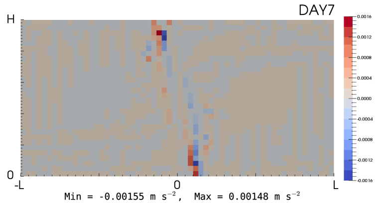
Figure 11: Residual in the out-of-slice velocity field calculated at day 7 of the control run.

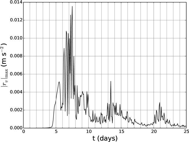
Figure 12: Time evolution of the maximum amplitude of the residual in the out-of-slice velocity field of the control run.

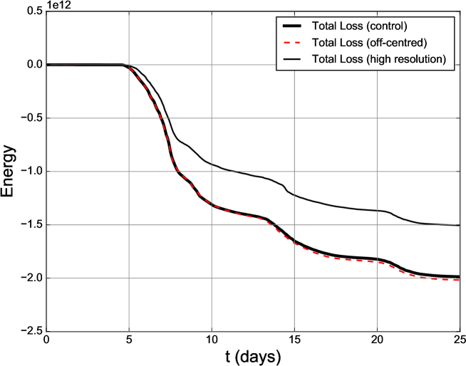
Figure 13: Comparison of the loss of total energy from the initial state in experiments with different settings. Thick line represents the same loss of total energy of the control run as in Figure 10. Dashed line shows the loss when using $\alpha$ = 0.55. Thin line represents the loss in the high-resolution run.

Finally, Figure 13 provides a comparison of the loss of total energy in the experiments performed in the previous sections. Note that with all three results shown in Figure 13 the rescaling factor $\beta$ is unity. The thick line shows the same loss of total energy from the initial state in the control run as in Figure 10. The dashed line shows the loss of the total energy in the experiment with off-centring, which is performed in section 3.2. It is shown that the use of off-centring has an insignificant effect on the loss of energy. This result, together with the results in Figures 6(b) and 7(b), suggests that off-centring does not have a big impact on the large scale dynamics but the unbalanced motion. The thin solid curve in Figure 13 represents the loss of total energy in the high-resolution run, which is performed in section 3.1. There is a clear improvement in energy conservation with the use of the high resolution; the total loss at day 25 is about 25 % less than that of the control run. It supports our assumption that the lack of resolution is a significant cause of the loss of energy. However, as shown in Figure 5, the high-resolution run gives only a slight increase in the peak amplitudes of RMSV despite the improvement in energy conservation. Therefore we have concluded that the energy loss in the model does not account for the large gap between the model result and the SG limit solution on RMSV.

4 Conclusion

A new vertical slice model of nonlinear Eady waves was developed using a compatible finite element method. To extend the Charney-Phillips grid staggering in the compatible finite element framework, the buoyancy is chosen from the function space which has the same degrees of freedom as the vertical part of the velocity space. As the buoyancy space is discontinuous in the horizontal direction and continuous in the vertical direction, we proposed a blend of an upwind DG method in the horizontal direction and SUPG method in the vertical direction.

The model reproduced several quasi-periodic lifecycles of fronts despite the presence of strong discontinuities. The general results of frontogenesis are consistent with the early studies. To validate the numerical implementation and assess the long term performance of the model, the asymptotic convergence to the SG limit solution is examined. Despite the large difference with the SG solution in RMSV, the solutions of the vertical slice model were converging to a solution in geostrophic balance as the Rossby number was reduced. With off-centring, the model showed the expected second-order convergence rate from the early stage up to the formation of the discontinuity, and showed a first-order rate for some time afterwards. This result is comparable to the previous results using a finite difference semi-implicit semi-Lagrangian method (Visram et al., 2014), indicating that the compatible finite element method is performing well for this test problem. In particular, the use of Eulerian advection schemes rather than semi-Lagrangian schemes does not degrade the results.

The energy analysis showed that the model suffers from dissipation of kinetic energy of the cross-front velocity due to the lack of resolution at the fronts in the $v$ advection scheme. However, the energy loss is very small compared to the amplitudes of potential energy and kinetic energy of the cross-front velocity, and is unlikely to account for the large gap between the RMSV values of the model and the SG limit. The large gap corresponds more likely to the fact that the lack of resolution shuts off the growth of the RMSV of the model about two days early compared to that of the SG limit. As the frontal discontinuity reaches the grid scale very quickly, we would need resolution of several orders of magnitude greater than presently used to reach the RMSV of the SG solution.

The frontogenesis test case shown in this paper demonstrates several aspects of the compatible finite element framework including the treatment of advection terms in the velocity equation, and an advection scheme for the vertically-staggered temperature space proposed here. In concurrent research we are incorporating these techniques into a discretisation of the compressible Euler equations for NWP, and the formulation and test cases will be reported in a future paper. For a scalable solution approach for the implicit linear system in (60)–(63), we are currently developing a hybridisation capability within the Firedrake package and intend to use this in future versions of the code. As an extension of the vertical slice modelling of nonlinear Eady waves, we are also considering a development of a parameterisation scheme which could prevent the model shutting off the growth of the RMSV too early, so that we could increase the peak amplitudes of the fronts without using unrealistically high resolution.

References

- Amestoy et al. (2001) Amestoy, P. R., Duff, I. S., L’Excellent, J.-Y., Koster, J., 2001. A fully asynchronous multifrontal solver using distributed dynamic scheduling. SIAM Journal on Matrix Analysis and Applications 23 (1), 15–41.
- Amestoy et al. (2006) Amestoy, P. R., Guermouche, A., L’Excellent, J.-Y., Pralet, S., 2006. Hybrid scheduling for the parallel solution of linear systems. Parallel Computing 32 (2), 136–156.
- Arakawa and Lamb (1977) Arakawa, A., Lamb, V. R., 1977. Computational design of the basic dynamical processes of the UCLA general circulation model. Methods in Computational Physics 17, 173–265.
- Bao et al. (2015) Bao, L., Klöfkorn, R., Nair, R. D., 2015. Horizontally explicit and vertically implicit (HEVI) time discretization scheme for a discontinuous Galerkin nonhydrostatic model. Monthly Weather Review 143 (3), 972–990.
- Brdar et al. (2013) Brdar, S., Baldauf, M., Dedner, A., Klöfkorn, R., 2013. Comparison of dynamical cores for NWP models: comparison of COSMO and Dune. Theoretical and Computational Fluid Dynamics 27 (3-4), 453–472.
- Budd et al. (2013) Budd, C. J., Cullen, M., Walsh, E., 2013. Monge–ampére based moving mesh methods for numerical weather prediction, with applications to the Eady problem. Journal of Computational Physics 236, 247–270.
-
COFFEE (2016)
COFFEE, Oct. 2016. COFFEE: A Compiler for Fast Expression Evaluation.
URL https://doi.org/10.5281/zenodo.161506 - Cotter and Holm (2013) Cotter, C., Holm, D., 2013. A variational formulation of vertical slice models. Proceedings of the Royal Society of London A: Mathematical, Physical and Engineering Sciences 469 (2155), 20120678.
- Cotter and Kuzmin (2016) Cotter, C., Kuzmin, D., 2016. Embedded discontinuous Galerkin transport schemes with localised limiters. Journal of Computational Physics 311, 363–373.
- Cotter and Shipton (2012) Cotter, C., Shipton, J., 2012. Mixed finite elements for numerical weather prediction. Journal of Computational Physics 231 (21), 7076–7091.
- Cotter and Thuburn (2014) Cotter, C. J., Thuburn, J., 2014. A finite element exterior calculus framework for the rotating shallow-water equations. Journal of Computational Physics 257, 1506–1526.
- Cullen (2007) Cullen, M., 2007. Modelling atmospheric flows. Acta Numerica 16, 67–154.
- Cullen (2008) Cullen, M., 2008. A comparison of numerical solutions to the Eady frontogenesis problem. Quarterly Journal of the Royal Meteorological Society 134 (637), 2143–2155.
- Dennis et al. (2012) Dennis, J. M., Edwards, J., Evans, K. J., Guba, O., Lauritzen, P. H., Mirin, A. A., St-Cyr, A., Taylor, M. A., Worley, P. H., 2012. CAM-SE: A scalable spectral element dynamical core for the Community Atmosphere Model. The International Journal of High Performance Computing Applications 26 (1), 74–89.
-
Eady (2016)
Eady, Nov. 2016. Supporting software for ”Vertical slice modelling of
nonlinear Eady waves using a compatible finite element method”.
URL https://doi.org/10.5281/zenodo.166269 -
FIAT (2016)
FIAT, Oct. 2016. FIAT: The Finite Element Automated Tabulator.
URL https://doi.org/10.5281/zenodo.161508 -
Firedrake (2016)
Firedrake, Oct. 2016. Firedrake: an automated finite element system.
URL https://doi.org/10.5281/zenodo.161510 - Fournier et al. (2004) Fournier, A., Taylor, M. A., Tribbia, J. J., 2004. The spectral element atmosphere model (SEAM): High-resolution parallel computation and localized resolution of regional dynamics. Monthly Weather Review 132 (3), 726–748.
- Giraldo et al. (2013) Giraldo, F. X., Kelly, J. F., Constantinescu, E., 2013. Implicit-explicit formulations of a three-dimensional nonhydrostatic unified model of the atmosphere (NUMA). SIAM Journal on Scientific Computing 35 (5), B1162–B1194.
- Hoskins and Bretherton (1972) Hoskins, B. J., Bretherton, F. P., 1972. Atmospheric frontogenesis models: Mathematical formulation and solution. Journal of the Atmospheric Sciences 29 (1), 11–37.
- Kelly and Giraldo (2012) Kelly, J. F., Giraldo, F. X., 2012. Continuous and discontinuous Galerkin methods for a scalable three-dimensional nonhydrostatic atmospheric model: Limited-area mode. Journal of Computational Physics 231 (24), 7988–8008.
- Mardal and Winther (2011) Mardal, K.-A., Winther, R., 2011. Preconditioning discretizations of systems of partial differential equations. Numerical Linear Algebra with Applications 18 (1), 1–40.
- Marras et al. (2015) Marras, S., Kelly, J. F., Moragues, M., Müller, A., Kopera, M. A., Vázquez, M., Giraldo, F. X., Houzeaux, G., Jorba, O., 2015. A review of element-based Galerkin methods for numerical weather prediction: Finite elements, spectral elements, and discontinuous Galerkin. Archives of Computational Methods in Engineering, 1–50.
- Marras et al. (2013) Marras, S., Moragues, M., Vázquez, M., Jorba, O., Houzeaux, G., 2013. Simulations of moist convection by a variational multiscale stabilized finite element method. Journal of Computational Physics 252, 195–218.
- McRae and Cotter (2014) McRae, A. T., Cotter, C. J., 2014. Energy-and enstrophy-conserving schemes for the shallow-water equations, based on mimetic finite elements. Quarterly Journal of the Royal Meteorological Society 140 (684), 2223–2234.
- Nakamura (1994) Nakamura, N., 1994. Nonlinear equilibration of two-dimensional Eady waves: Simulations with viscous geostrophic momentum equations. Journal of the Atmospheric Sciences 51 (7), 1023–1035.
- Nakamura and Held (1989) Nakamura, N., Held, I. M., 1989. Nonlinear equilibration of two-dimensional Eady waves. Journal of the Atmospheric Sciences 46 (19), 3055–3064.
- Natale and Cotter (2016) Natale, A., Cotter, C. J., 2016. A variational H(div) finite element discretisation for perfect incompressible fluids. arXiv preprint arXiv:1606.06199.
-
Natale et al. (2016)
Natale, A., Shipton, J., Cotter, C. J., 2016. Compatible finite element spaces
for geophysical fluid dynamics. Dynamics and Statistics of the Climate
System.
URL https://doi.org/10.1093/climsys/dzw005 -
PETSc (2016)
PETSc, Oct. 2016. PETSc: Portable, Extensible Toolkit for Scientific
Computation.
URL https://doi.org/10.5281/zenodo.161513 -
petsc4py (2016)
petsc4py, Oct. 2016. petsc4py: The Python interface to PETSc.
URL https://doi.org/10.5281/zenodo.161512 -
PyOP2 (2016)
PyOP2, Oct. 2016. PyOP2: Framework for performance-portable parallel
computations on unstructured meshes.
URL https://doi.org/10.5281/zenodo.161511 - Rathgeber et al. (2016) Rathgeber, F., Ham, D. A., Mitchell, L., Lange, M., Luporini, F., McRae, A. T., Bercea, G.-T., Markall, G. R., Kelly, P. H., 2016. Firedrake: automating the finite element method by composing abstractions. ACM Transactions on Mathematical Software (TOMS) 43 (3), 24.
- Raymond and Garder (1976) Raymond, W. H., Garder, A., 1976. Selective damping in a Galerkin method for solving wave problems with variable grids. Monthly Weather Review 104 (12), 1583–1590.
- Shu and Osher (1988) Shu, C.-W., Osher, S., 1988. Efficient implementation of essentially non-oscillatory shock-capturing schemes. Journal of Computational Physics 77 (2), 439–471.
- Snyder et al. (1993) Snyder, C., Skamarock, W. C., Rotunno, R., 1993. Frontal dynamics near and following frontal collapse. Journal of the Atmospheric Sciences 50 (18), 3194–3212.
- Staniforth et al. (2013) Staniforth, A., Melvin, T., Cotter, C., 2013. Analysis of a mixed finite-element pair proposed for an atmospheric dynamical core. Quarterly Journal of the Royal Meteorological Society 139 (674), 1239–1254.
- Thomas and Loft (2005) Thomas, S. J., Loft, R. D., 2005. The NCAR spectral element climate dynamical core: Semi-implicit Eulerian formulation. Journal of Scientific Computing 25 (1), 307–322.
-
TSFC (2016)
TSFC, Oct. 2016. TSFC: The Two Stage Form Compiler.
URL https://doi.org/10.5281/zenodo.161507 -
UFL (2016)
UFL, Oct. 2016. UFL: The Unified Form Language.
URL https://doi.org/10.5281/zenodo.161509 - Visram (2014) Visram, A., 2014. Asymptotic limit analysis for numerical models of atmospheric frontogenesis. PhD thesis, Imperial College London, 238.
- Visram et al. (2014) Visram, A., Cotter, C., Cullen, M., 2014. A framework for evaluating model error using asymptotic convergence in the Eady model. Quarterly Journal of the Royal Meteorological Society 140 (682), 1629–1639.
- Williams (1967) Williams, R., 1967. Atmospheric frontogenesis: A numerical experiment. Journal of the Atmospheric Sciences 24 (6), 627–641.
- Wood et al. (2014) Wood, N., Staniforth, A., White, A., Allen, T., Diamantakis, M., Gross, M., Melvin, T., Smith, C., Vosper, S., Zerroukat, M., et al., 2014. An inherently mass-conserving semi-implicit semi-lagrangian discretization of the deep-atmosphere global non-hydrostatic equations. Quarterly Journal of the Royal Meteorological Society 140 (682), 1505–1520.