Abstract

We propose a novel general approach to locality of lattice composite fields, which in case of QCD involves locality in both quark and gauge degrees of freedom. The method is applied to gauge operators based on the overlap Dirac matrix elements, showing for the first time their local nature on realistic path-integral backgrounds. The framework entails a method for efficient evaluation of such non-ultralocal operators, whose computational cost is volume-indepenent at fixed accuracy, and only grows logarithmically as this accuracy approaches zero. This makes computation of useful operators, such as overlap-based topological density, practical. The key notion underlying these features is that of exponential insensitivity to distant fields, made rigorous by introducing the procedure of statistical regularization. The scales associated with insensitivity property are useful characteristics of non-local continuum operators.

1 Introduction

Local quantum field theories are quantum field systems with dynamics prescribed by local action density. When such theories serve to describe particle interactions then, in addition, $n$-point correlation functions of local operators encode most of the interesting observables. The notion of a local operator is thus deeply engrained in these descriptions.

Locality is rarely viewed as problematic or subtle in formal continuum considerations. Indeed, the presence of space-time derivatives invokes confidence that field variables separated by non-zero distance are not explicitly coupled by the operator, consistently with the intuitive meaning of locality. However, the concept becomes richer once an actual definition of the theory, such as via lattice regularization which we follow here, is carried out.

A common approach to formulating lattice-regularized systems is to replace space-time field derivatives with nearest-neighbor field differences. More generally, operators that only depend on field variables within fixed lattice distance away from each other are referred to as ultralocal. However, lattice operators with couplings extending to arbitrary distances naturally arise in Wilson’s renormalization group considerations. Moreover, chirality-preserving Dirac operators of Ginsparg-Wilson type [1] are all of such non-ultralocal variety [2, 3]. Locality becomes a more subtle notion in these situations, and requires some care.

In this work, we consider non-ultralocal operators associated with overlap Dirac matrix $D\equiv\{D_{x,y}(U)\}$ [4] in the context of QCD. Here the color-spin indices are implicit and $U\equiv\{U_{x,\mu}\}$ is the SU(3) lattice gauge field. There are at least two relevant circumstances to consider. Firstly, since $\sum_{x}{\bar{\psi}}_{x}(D\psi)_{x}$ prescribes interactions of quarks and gluons, it is required to be a sum of local contributions. Operator $(D\psi)_{x}$ thus has to be local with respect to both fermionic and gauge variables. Secondly, there are interesting gauge operators based on overlap matrix elements, such as topological charge density [5, 6], gauge action density [7, 8, 9] or gauge field strength tensor [7, 10] constructed from $D_{x,x}(U)$. To be used in well-founded QCD calculations, these objects need to be local in gauge potentials.

While fermionic locality of the overlap operator was studied in some detail [11], the aspects of gauge locality have barely been considered. In fact, they were not studied at all for realistic gauge fields of lattice QCD ensembles. The theme of the present work is to examine this issue, especially in relation to the above non-ultralocal gauge operators. The novelty of our approach is that it naturally connects locality of an operator to efficiency achievable in its evaluation. Consequently, the results that follow have direct bearing on the practical use of these computationally demanding objects.

To start describing our approach, recall that the modern notion of locality for lattice-defined operators includes their exponentially decreasing sensitivity to distant field variables. Standard treatment formalizes this into exponential bound on the corresponding field derivatives. For example, fermionic locality of $(D\psi)_{x}$ then simply requires sufficiently fast decay of $D_{x,y}$ as $y$ is taken increasingly far away from $x$. Albeit less elegant due to gauge field entering in a more complicated manner, this prescription can also be followed to study gauge locality of $(D\psi)_{x}$ or locality of $D_{x,x}(U)$.

However, for our purposes it is fruitful to replace the above “differential” treatment of dependence on distant fields with a direct “integral” approach. In other words, we ask how well is it possible to know the value of a composite operator $O_{x}$ when the knowledge of fundamental fields is restricted to some neighborhood of $x$. Exponentially suppressed sensitivity to distant fields is then formalized as the existence of estimates whose precision exponentially improves with the linear extent of these neighborhoods.

To explain this in more detail, consider operators $O_{x}$ that only depend on the gauge field, such as covariant discretizations of $F\tilde{F}(x)$. The simplest ultralocal option is based on minimal gauge loops (plaquettes), but general $O_{x}(U)$ may couple fields everywhere. We will use hypercubic neighborhoods of $x$ with “radius” $r$ to define patches $U^{x,r}\subset U$ of the field, as illustrated in Fig. 1. Note that $r\!=\!ja$ is discrete at finite lattice cutoff $a$. Faced with the task of estimating $O_{x}(U)$ given an incomplete knowledge ($U^{x,r}$) of its argument, one is led to construct approximants $O_{x}^{r}(U)=O_{x}^{r}(U^{x,r})$ depending only on variables in the patch. If ${\delta}(r,U)\equiv\|O_{x}(U)-O_{x}^{r}(U)\|$ denotes the associated error, one may choose to formalize exponential insensitivity to distant fields of $O_{x}$ by requiring the existence of $O_{x}^{r}$ and finite positive constants $B$, $R$, $s$ such that

$${\delta}(r,U)\,\leq\,B\exp\left(-r/R\,\right)\quad\;,\;\quad r\geq s\quad\;,\;\quad\forall\,U$$ (1)

But the notion so construed is unnecessarily strong since violations of (1) involving configurations $U$ that are statistically irrelevant in the path integral, are inconsequential in the context of corresponding quantum theory. We thus replace condition (1) by

$${\delta}(r,p)\,\leq\,B\exp\left(-r/R\,\right)\quad\;,\;\quad r\geq s\quad\;,\;\quad\forall\,p<1$$ (2)

where ${\delta}(r,p)$ is a statistical construct representing “error with probability $p$”, effectively demanding that the bound is satisfied up to events of probabilistic measure zero. In the resulting procedure of statistical regularization, the bound is examined at fixed certainty $p$, and this cutoff is eventually lifted via the appropriate $p\!\to\!1$ limit (Sec.2). Note that tying exponential insensitivity of an operator to path integral in which it is used implies that minimal sensitivity range $R\!\to\!R_{0}$ can have non-trivial dependence on the lattice spacing. Locality then requires, among other things, that $R_{0}(a)$ vanishes in the continuum limit.

           

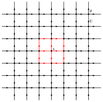
Figure 1: Gauge field patch involved in simplest gauge covariant operators $O_{x}$ (left) and the geometry of hypercubic neighborhoods with radius $r$ (right).

The notion of exponential insensitivity, outlined above, admits arbitrary $O_{x}^{r}$ to be considered in Eq. (2). However, if the property holds for $O_{x}$, the facilitating approximant is clearly not unique, and different options may involve widely varied degrees of computational complexity. In fact, albeit coupling fewer degrees of freedom, computational demands for most precise choices of $O_{x}^{r}$ can be as large or larger than those for $O_{x}$ itself. However, our goal here is not to determine the best approximation. Rather, we are interested in finding $O_{x}^{r}$ whose computational complexity scales with $r/a$ in qualitatively the same manner as that of $O_{x}$ with $L/a$. Here $L\!\gg\!r$ is the size of the system. Apart from demonstrating exponential insensitivity, the existence of such approximants would offer great computational advantage. Indeed, if the program computing $O_{x}$ has no a priori knowledge about insensitivity, then single evaluation incurs cost growing at least with the lattice 4-volume for non-ultralocal operators of interest here. This is reduced as

$$\Bigl{(}\,\frac{L}{a}\,\Bigr{)}^{4+\alpha}\quad\longrightarrow\quad\Bigl{(}\,\frac{R}{a}\,\log\frac{B}{{\delta}}\Bigr{)}^{4+\alpha^{\prime}}\quad,\quad\alpha,\alpha^{\prime}\geq 0$$ (3)

for the approximant that guarantees absolute precision ${\delta}$. Computation could thus be performed at a constant cost (independent of the volume) that only depends logarithmically on the desired precision.

Our suggestion for constructing generic and practical approximants $O_{x}^{r}$ of the above type is to treat the neighborhood containing $U^{x,r}$ as a finite system of its own. Indeed, definition of non-ultralocal $O_{x}$ implicitly involves a sequence of operators: one for each space-time lattice involved in the process of taking the infinite-volume limit. Considering $L^{4}$ lattices and making the $L$-dependence explicit for the moment ($O_{x}\rightarrow O_{x,L}$), the replacement

$$O_{x,L}(U)\quad\longrightarrow\quad O_{x,L\to 2r+a}(U^{x,r})\;\equiv\;O_{x}^{r}(U^{x,r})\,=\,O_{x}^{r}(U)$$ (4)

offers a generic scheme for obtaining candidate approximants. Note that $L/a$ is defined to count the sites and hence $2r\!+\!a$ is the “size” of the lattice system contained in hypercubic neighborhood with radius $r$. Variations on this prescription discussed in the body of the paper correspond to different treatment of boundaries in the subsystem associated with the patch. We refer to approximants of type (4) as boundary approximants since they test sensitivity to the boundary created by the restriction $U\rightarrow U^{x,r}$. If they exhibit the behavior (2), then $O_{x}$ is exponentially insensitive to distant fields, and a stronger notion of locality (boundary locality) can be built around this concept.

The paper is organized as follows. In Sec. 2 we introduce the concept of exponential insensitivity to distant fields via statistical regularization. Given its pivotal role in the present discussion, this is carried out in detail so that relevantly distinct behaviors are discerned, and the subtleties known to us are all accounted for. A notable feature of the resulting framework is that the removal of lattice and statistical cutoffs necessitates not only a non-divergent exponential range $R_{0}$, but also a non-divergent auxiliary (non-unique) scale ${\rho}_{0}$ representing the threshold distance for validity of the bound. This part concludes with connecting the locality to exponential insensitivity and defining it correspondingly. In Sec. 3 the stronger notions of boundary insensitivity and boundary locality are put forward, emphasizing their practical relevance. In particular, the consequences of this property for efficient evaluation of computable non-ultralocal operators is discussed in detail. The possibility that suitably constructed boundary approximant can also serve as a standalone ultralocal operator, interesting in its own right, is suggested here as well. In Sec. 4 we investigate the properties of basic overlap-based gauge operators in the proposed framework. Our numerical results in pure glue theory readily show the weak form of insensitivity (for any fixed statistical cutoff) at the lattice level, and the corresponding weak form of locality in the continuum. They also lend an initial support to full insensitivity (statistical cutoff removed) sufficiently close to the continuum limit, and the associated locality. To illustrate the practical aspects of exponential insensitivity, we discuss in Sec. 5 the use of boundary approximants for efficiently computing the “configurations” of overlap-based topological density. This lattice topological field was crucial for identifying the low-dimensional long-range topological structure in QCD vacuum [12]. The insensitivity properties tested here make large scale computations of this type practical since, at fixed accuracy, the cost per configuration is simply proportional to the volume, similarly to the case of generic ultralocal gauge operators.

2 Exponential Insensitivity to Distant Fields

The concept of exponential insensitivity to distant fields is central to this work, and we thus begin by working out the necessary details. The issues in need of attention arise mostly due to the quantum setting we are dealing with. To see this, consider some extended operator (functional) $O_{x}[A]$ of gauge fields $A\!\equiv\!\{A_{\mu}(y)\}$ in the continuum space-time. The analog of Eq. (1), involving spherical neighborhoods of $x$ in Euclidean space, is intended to characterize exponential insensitivity of $O_{x}$. However, the required bound may not hold, or even be meaningful, for arbitrary $A$, and yet be satisfied by a subset of fields relevant to the situation at hand. Indeed, the proper definition requires specifying the class of fields in question. Problems involving classical dynamics of $O_{x}$ naturally come with needed analytic restrictions since they deal with fields $A$ obeying classical equations of motion.

However, in field theory regularized and quantized via lattice path integral, there is no a priori restriction on the fundamental fields (“configurations”) $U$: there is only a hierarchy induced by their statistical weights. While this forces one to adopt the notion of exponential insensitivity involving all lattice fields in principle, it also makes room for the concept to be viable even when there are sufficiently improbable configurations violating any exponential bound. Indeed, we are led to a statistical approach respecting the path integral hierarchy of fields and, at the same time, facilitating the systematic separation of potential outliers in the process we refer to as statistical regularization. Its idea is to replace the sharp construct of least upper bound with the statistical “least upper bound with probability $p$”. Before defining the concept in Sec.2.3, we need to discuss some preliminaries.

2.1 The Setup

Unless stated otherwise, the position coordinates of an underlying infinite system are spanned by entire $d$-dimensional hypercubic lattice with cutoff $a$, i.e.

$${\cal H}_{\infty}\equiv\{\,x\mid\,x_{\mu}\!=\!an_{\mu}\,,\,n_{\mu}\in{\mathbb{Z}}\,,\,\mu=1,2,\ldots,d\,\}$$ (5)

The general case where infinite volume involves a subset of points in ${\cal H}_{\infty}$ is described in Appendix D, and allows e.g. for applying our methods to arbitrary spatial geometry, or to theories at finite temperature. The hypercubic neighborhood of point $x$ with radius $r$ is

$${\cal H}^{x,r}\equiv\{\;y\in{\cal H}_{\infty}\;\mid\;|x_{\mu}-y_{\mu}|\leq r\;,\;\forall\mu\;\}\qquad\qquad r\in\{\,ja\,\mid\,j=1,2,3,\ldots\,\}\equiv{\mathbb{N}}_{a}$$ (6)

We consider operator $O_{x}\!=\!O_{x}(U)$, composed of gauge field $U\!\equiv\!\{U_{y,\mu}\}$, in theory defined by $S(U)$, namely the effective gauge action after integrating out quark fields, if any. This quantum dynamics is infrared-regularized on symmetric lattices of $(L/a)^{4}$ sites centered around $x$, i.e. the center of the lattice is at $x$ for $L/a$ odd, and at $x+(a/2,\ldots,a/2)$ for $L/a$ even. Each ${\cal H}^{x,r}$ contained within given finite system is assigned a hypercubic field patch

$$U^{x,r}\equiv\{\;U_{y,\mu}\in U\;\mid\;\;y,y\!+\!{\hat{\mu}}\,\in\,{\cal H}^{x,r}\;\}\;,\qquad\;2r+a<L$$ (7)

Note that $U^{x,r}$ doesn’t include links “dangling” with respect to ${\cal H}^{x,r}$. For example, the set of red links in Fig.1 (left) is $U^{x,r=a}$. Any operator $O_{x}^{r}$ with range in the normed space of $O_{x}$ and satisfying $O_{x}^{r}(U)\!=\!O_{x}^{r}(U^{x,r})$, will be referred to as approximant of $O_{x}$ with radius $r$.

2.2 Kinematics of Exponential Bounds

Important technical aspect of the analysis that follows involves sufficiently detailed description of exponential bounds which we now discuss. Generic real-valued “error function”

$$0\leq{\delta}(r)<\infty\qquad,\qquad r\in{\mathbb{N}}_{a}$$ (8)

is said to be exponentially boundable if there are finite positive $R$, $\Delta$, $s$ such that

$${\delta}(r)\,\leq\,\Delta\,\exp\left(-\frac{r-s}{R}\,\right)\quad\;,\;\quad r\geq s\in{\mathbb{N}}_{a}$$ (9)

Note that, in this form, the prefactor $\Delta$ specifies the bound at threshold distance $s$. Our goal is to identify a region in parameter space $R\!>\!0$, $\Delta\!>\!0$, $s\!\in\!{\mathbb{N}}_{a}$, if any, where (9) holds.

Explicit solution to this problem is obtained by rewriting (9) as

$$\Delta\;\geq\;\exp\left(-s/R\right)\;\,\sup\,\{\,{\delta}(r)\,\exp\left(r/R\right)\,\mid\,r\geq s\,\}\;\equiv\;\Delta_{0}(R,s)$$ (10)

Thus, for given $(R,s)$, the indicated range of valid $\Delta$ materializes, as long as $\Delta_{0}(R,s)<\infty$. At the same time, finiteness of $\Delta_{0}(R,s)$ only depends on $R$. Indeed, $s\to s^{\prime}$ induces at most a finite change in $\Delta_{0}$ since the sets involved in suprema only differ by finite number of finite elements. Consequently, the following defines an $s$-independent object

$$R_{0}\;\equiv\;\inf\,\{\,R>0\,\mid\,\Delta_{0}(R,s)<\infty\,\}\;\geq\;0$$ (11)

namely the effective range of ${\delta}(r)$. Exponential boundability of ${\delta}(r)$ is equivalent to $R_{0}<\infty$, and the parameter domain of validity for (9) is $R>R_{0}$, $s\in{\mathbb{N}}_{a}$, $\Delta\geq\Delta_{0}(R,s)$. We will work with description of this domain in which the threshold error $\Delta$, rather than threshold distance $s$, enters as an unconstrained free parameter. Since $\Delta_{0}(R,s)$ is decreasing in $s$, and $\lim_{s\to\infty}\Delta_{0}(R,s)=0$, its “inverse” defines the desired representation, namely

$$R>R_{0}\quad\qquad\Delta>0\quad\qquad s\geq s_{0}(R,\Delta)\;\equiv\;\min\,\{\,r\,\mid\,\Delta_{0}(R,r)\leq\Delta\,\}$$ (12)

Function $s_{0}(R,\Delta)$ is a core size outside of which a bound with desired $(R,\Delta)$ sets in.

This detailed kinematics of exponential bounds acquires relevance in quantum setting, where ultraviolet and statistical regularizations produce error functions depending on associated cutoffs. It turns out that monitoring cutoff dependence of $R_{0}$ alone is not sufficient to ensure requisite bounds upon regularization removal, and information in $s_{0}$ is also needed. To that end, it is useful to treat $s_{0}$ as a continuous entity (like $R_{0}$) so that trends can be detected even for small changes in the cutoffs. We thus extend $\Delta_{0}(R,s)$ at fixed $R$, into a decreasing continuous map $\Delta_{0}(R,{\rho})$ from ${\rho}\!\in\!(0,\infty)$ onto $(0,\infty)$. Omitting the $R$-dependence, the exponential behavior of $\Delta_{0}(s)$ motivates a practical choice

$$\log\Delta_{0}({\rho})\equiv\begin{cases}\text{\tt Lin}\,\bigl{(}\,\log\Delta_{0}(s)\,,\,{\rho}\,\bigr{)}&\text{for }{\rho}\geq a\\ -1+a/{\rho}+\log\Delta_{0}(a)&\text{for }{\rho}<a\end{cases}$$ (13)

where Lin $\!(f(s),{\rho})$ denotes linear interpolation of $f(s)$ via variable ${\rho}$. The arbitrary completion for ${\rho}\!<\!a$ only serves to realize the desired range. With $\Delta_{0}(R,{\rho})$ so fixed, the associated core-size function ${\rho}_{0}(R,\Delta)$ is uniquely defined via $\Delta_{0}(R,{\rho}_{0})\!=\!\Delta$, guaranteeing that

$${\delta}(r)\,\leq\,\Delta\,\exp\left(-\frac{r-{\rho}}{R}\,\right)\quad\;\text{for}\quad\;r\geq{\rho}\quad\quad R>R_{0}\quad\quad\Delta>0\quad\quad{\rho}\geq{\rho}_{0}(R,\Delta)$$ (14)

Note that setting $R\!=\!R_{0}$ to optimize the bound at large distances is not always possible since ${\rho}_{0}(R,\Delta)$ may diverge for $R\!\to\!R_{0}^{+}$. This occurs when ${\delta}(r)$ decays as an exponential modulated by an unbounded function, e.g. ${\delta}(r)\propto r\exp(-r/R_{0})$. Such cases require $R$ in (14) that may be arbitrarily close but larger than $R_{0}$, as indicated. However, setting ${\rho}\!=\!{\rho}_{0}(R,\Delta)$, whenever finite, always produces a valid bound

$${\delta}(r)\,\leq\,\Delta\,\exp\left(-\frac{r-{\rho}_{0}(R,\Delta)}{R}\,\right)\qquad,\qquad r\geq{\rho}_{0}(R,\Delta)$$ (15)

Vice versa, when ${\rho}_{0}(R,\Delta)$ is ill-defined (infinite), there is no exponential bound involving range $R$ and threshold error $\Delta$. The core-size function is thus a master construct containing complete information on exponential bounds of ${\delta}(r)$. The bounds in 2-parameter family (15) are optimal in that they cover the maximal range of distances for given $(R,\Delta)$.

2.3 Statistical Regularization

Given a composite field $O_{x}(U)$ and its approximant $O_{x}^{r}(U)=O_{x}^{r}(U^{x,r})$, the properties of the latter are described by distribution $P_{r}({\delta})$ of its errors over the path integral ensemble. The corresponding cumulative probability function $F_{r}({\delta})$ is explicitly given by

$$F_{r}({\delta})\equiv\Big{\langle}\,H\,\Big{(}\,{\delta}-\|O_{x}(U)-O_{x}^{r}(U)\|\,\Big{)}\,\Big{\rangle}\qquad\qquad P_{r}({\delta})\equiv\frac{d}{d{\delta}}F_{r}({\delta})$$ (16)

with $H$ denoting a Heaviside step function and $\langle\ldots\rangle$ the path integral average specified by $S(U)$. This information can be recast into error bounds ${\delta}(r,p)$ satisfied by fractions $p$ of the overall population with smallest deviations by imposing

$$F_{r}\Big{(}{\delta}(r,p)\Big{)}\equiv p$$ (17)

i.e. by inverting $F_{r}({\delta})$. By construction, the meaning of ${\delta}(r,p)$ is that of an “error bound with probability $p$”: if $O_{x}^{r}$ is used to estimate $O_{x}$, the expected error is less than ${\delta}(r,p)$ with probability $p$. This family of error functions is central to the analysis proposed here.

For $O_{x}$ to exhibit exponential insensitivity to distant fields, statistically regularized by fixed $0\!<\!p\!<\!1$, we require that ${\delta}(r,p)$ decays at least exponentially at asymptotically large $r$, i.e. that it is exponentially boundable. The advertised “separation of potential outliers” is thus accomplished by fixing the degree of certainty $p$ in examining the influence of distant fields on error. Examples of measured $r$-dependencies for several overlap-based operators are shown in Fig. 2, with details described in Sec. 3. The observed behavior is clearly compatible with exponential falloff at rates depending very weakly (if at all) on $p$.

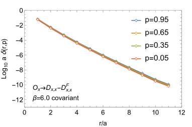
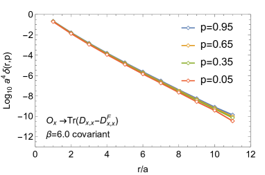
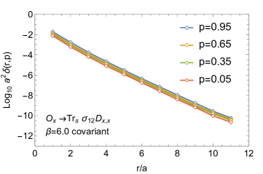
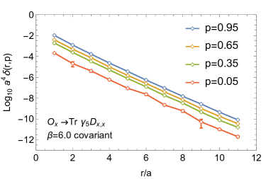
Figure 2: The behavior of ${\delta}(r,p)$ at fixed $p$ for overlap-based gauge operators (Sec. 4). Note that $\mathop{\rm Tr}\gamma_{5}D_{x,x}\propto q(x)$ (topological density) has the strongest dependence on $p$.

Exponential insensitivity at any non-zero $p$ is in itself (without $p\!\to\!1$ considerations) a notable feature of non-ultralocal lattice operator. Indeed, at minimum, it signals the existence of insensitive subpopulation in the path integral, which can be useful computationally and otherwise. We formalize this lattice concept as follows.

Definition 1 (exponential insensitivity at fixed $p$)

Let $O_{x}(U)$ be the operator with values in normed space and $S(U)$ the action of Euclidean gauge theory, both defined on hypercubic lattices of arbitrary size $L$. We say that $O_{x}$ is exponentially insensitive to distant fields with respect to $S$ at probability $p$, if there is an $r$-dependent approximant $O_{x}^{r}(U)=O_{x}^{r}(U^{x,r})$ such that

(i)

The infinite-volume limit ${\delta}(r,p)\equiv\lim_{L\to\infty}{\delta}(r,p,L)$ of its error function exists.

(ii)

${\delta}(r,p)$ is exponentially boundable.

Here $U^{x,r}$ is the patch of $U$ contained in hypercubic neighborhood of $x$ with radius $r$. $\quad\Box$

This definition categorizes lattice operators at given position in terms of their dependence on remote fields. Abbreviating exponential insensitivity to distant fields as “insensitivity”, if there is no $p\!>\!0$ at which $O_{x}$ is insensitive, then $O_{x}$ is sensitive, while in the opposite case it is said to contain an insensitive component. When the latter holds for all $p\!<\!1$ then $O_{x}$ is referred to as weakly insensitive provided that the “outliers” do not contribute finitely to $O_{x}$ in $p\!\to\!1$ limit. Weakly insensitive operator is under exponential control with any preset probability short of certainty which, among other things, can provide a powerful advantage for its evaluation. Finally, if removing statistical cutoff ($p\!\to\!1$) in weakly insensitive $O_{x}$ leaves some exponential bounds in place, we speak of insensitive operator. However, the process of cutoff removal needs to be specified and discussed in some detail.

2.4 The Removal of Statistical Cutoff

Imposing the statistical cutoff $p$ turns a quantum situation, involving path integral over fields, into classical-like setting specified by single error function ${\delta}(r,p)$. Regularized exponential insensitivity to distant fields is synonymous with its exponential boundability which, in turn, is equivalent to the associated effective range $R_{0}(p)$ being finite. It is thus tempting to conclude that $\lim_{p\to 1}R_{0}(p)\!<\!\infty$ is the proper requirement for weakly insensitive operator $O_{x}$ to be fully insensitive.

However, this cutoff-removal prescription is not sufficient because it doesn’t guarantee the existence of $p$-independent exponential bound. For example, consider the family of error functions ${\delta}(r,p)$ taking constant value $\Delta$ for $r\!\leq\!r_{0}(p)$, and decaying as pure exponential of range $R_{0}$ for $r\!>\!r_{0}(p)$. With $\Delta$ and $R_{0}$ being $p$-independent, if radius $r_{0}(p)$ of the constant core grows unbounded as the cutoff is lifted ($\lim_{p\to 1}r_{0}(p)\!=\!\infty$) then there is no exponential bound valid for all $p\!<\!1$, albeit the condition of finite limiting range is readily satisfied.

The possibility of such behavior should not be too surprising in light of our analysis in Sec. 2.2, and its result (14). Indeed, the subset of parameter space $(R,\Delta,{\rho})$ describing valid exponential bounds is determined not only by $R_{0}(p)$ but also by the core size ${\rho}_{0}(R,\Delta,p)$. Finiteness of both is needed in $p\!\to\!1$ limit, namely

$$\lim_{p\to 1}\,R_{0}(p)<\infty\qquad\quad\text{and}\qquad\quad\exists\;R>0\;,\;\Delta>0\quad:\quad\lim_{p\to 1}\,{\rho}_{0}(R,\Delta,p)<\infty$$ (18)

The example of previous paragraph violates the second condition which is, strictly speaking, alone sufficient for insensitivity since it implies finite limiting range. However, keeping both requirements explicit is more reflective of steps involved in determination of insensitivity in practice. The equivalent formal definition, given below, closely mimics this process and is tailored for the eventual step of ultraviolet cutoff removal. Instead of $(R,\Delta)$, this formulation specifies the bounds of ${\delta}(r,p)$ via relative parameters $(\kappa,\mathscr{E})$, namely

$$R=\kappa\,R_{0}(p)\;,\;\kappa>0\qquad\quad\Delta=\mathscr{E}\,\langle\,\|O_{x}\|\,\rangle\;,\;\mathscr{E}>0\qquad\quad{\rho}_{0}(R,\Delta,p)\rightarrow{\rho}_{0}(\kappa,\mathscr{E},p)$$ (19)

and monitors the finiteness of ${\rho}_{0}(\kappa,\mathscr{E},p)$ in $p\!\to\!1$ limit. At fixed $\kappa\!>\!1$, i.e. $\kappa R_{0}(p)\!>\!R_{0}(p)$, this limiting process is manifestly well-defined for weakly insensitive operator. Introduction of $\mathscr{E}$ corresponds to measuring the error in units of typical magnitude of the operator, which is inconsequential at fixed ultraviolet cutoff but essential for taking the continuum limit. Indeed, since the operator values depend on lattice spacing, a meaningful assessment of insensitivity is to be performed at fixed $\mathscr{E}$. Reparametrization (19) puts optimal bounds (15) of ${\delta}(r,p)$ into the form

$$\delta(r,p)\,\leq\,\mathscr{E}\,\langle\|O_{x}\|\rangle\,\exp\bigg{(}\!-\frac{r-{\rho}_{0}(\kappa,\mathscr{E},p)}{\kappa\,R_{0}(p)}\,\bigg{)}\qquad,\qquad r\geq{\rho}_{0}(\kappa,\mathscr{E},p)$$ (20)

and the aforementioned definition of exponential insensitivity is as follows.

Definition 2 (exponential insensitivity)

Let $O_{x}(U)$ be a weakly insensitive operator with respect to $S(U)$, implying the existence of approximants $O_{x}^{r}(U)=O_{x}^{r}(U^{x,r})$ characterized by finite length scales $R_{0}(p)$, ${\rho}_{0}(\kappa,\mathscr{E},p)$, for all $0\!<\!p\!<\!1$, $\kappa\!>\!1$, $\mathscr{E}\!>\!0$. If there is $O_{x}^{r}$ and $\kappa$, $\mathscr{E}$ for which the finite limits below exist

$$\lim_{p\to 1}\,R_{0}(p)\,\equiv\,R_{0}<\infty\qquad\;\text{and}\qquad\;\lim_{p\to 1}\,{\rho}_{0}(\kappa,\mathscr{E},p)\,\equiv\,{\rho}_{0}(\kappa,\mathscr{E})<\infty$$ (21)

we say that $O_{x}$ is exponentially insensitive with respect to $S$. $\quad\Box$

Note that the $p$-independent optimal bound for given $(\kappa,\mathscr{E})$ is obtained by inserting $R_{0}$ and ${\rho}_{0}(\kappa,\mathscr{E})$ into formula (20). There are two points regarding Definition 2 we wish to emphasize.

(i) It is shown in Appendix B that, if ${\rho}_{0}(\kappa,\mathscr{E})\!<\!\infty$, then ${\rho}_{0}(\kappa^{\prime},\mathscr{E}^{\prime})\!<\!\infty$ for all $(\kappa^{\prime},\mathscr{E}^{\prime})$ with $\mathscr{E}^{\prime}\!>\!0$ and $\kappa^{\prime}\!\geq\!\kappa$. Thus, the threshold relative error $\mathscr{E}$ remains an unconstrained free parameter to keep fixed in $p\!\to\!1$ limit: its choice is purely a matter of practical convenience. However, Appendix B also shows that finiteness of $\rho_{0}$ is not guaranteed for $1\!<\!\kappa^{\prime}\!<\!\kappa$. As a practical consequence, examining a single value ${\rho}_{0}(\kappa,\mathscr{E})$ is not always sufficient to determine insensitivity. Indeed, if ${\rho}_{0}(\kappa,\mathscr{E})$ is infinite, there may be $\kappa^{\prime}\!>\kappa$ for which ${\rho}_{0}(\kappa^{\prime},\mathscr{E})$ is finite.

(ii) As discussed in Sec. 2.2, there is a class of error functions ${\delta}(r,p)$ obeying an exponential bound with $R$ set to the effective range $R_{0}(p)$. In this case the $p\!\to\!1$ limiting procedure at $\kappa\!=\!1$ can be set up and examined. This, however, cannot be assumed in general.

2.5 The Removal of Ultraviolet Cutoff

The prescription of monitoring ${\rho}_{0}$ at fixed $(\kappa,\mathscr{E})$ as statistical cutoff is lifted ($p\!\to\!1$ limit), is directly applicable to the process of ultraviolet cutoff removal ($a\!\to\!0$ limit). Indeed, an uncontainable core can emerge in the process of continuum limit as well. The importance of fixing $\mathscr{E}$ is further underlined by the fact that $\langle\,\|O_{x}\|\,\rangle$ is $a$-dependent, making it imperative that the approximation error (and thus core size ${\rho}_{0}$) relates to this changing typical magnitude in fixed proportion.

We now formulate this precisely in order to classify continuum operators defined by arbitrary lattice prescriptions in terms of their sensitivity to distant fields. Making the dependence on lattice spacing explicit, the error function ${\delta}(r,p,a)$ assigned to the pair $O_{x}$ and $O_{x}^{r}$ depends on both cutoffs, as do the associated characteristics $R_{0}(p,a)$, ${\rho}_{0}(\kappa,\mathscr{E},p,a)$. Following the structure of our formalism at fixed ultraviolet cutoff, the first step is to define the continuum version of exponential insensitivity at fixed $p$.

Definition 3 (exponential insensitivity at fixed $p$ – continuum)

Let $O_{x}(U)$ be the lattice operator exponentially insensitive with respect to $S(U)$ at given $p$ and lattice spacings $0\!<\!a\!<\!a_{0}$ i.e. sufficiently close to the continuum limit. Thus, there exist approximants $O_{x}^{r}(U)=O_{x}^{r}(U^{x,r})$ with finite characteristics $R_{0}(p,a)$ and ${\rho}_{0}(\kappa,\mathscr{E},p,a)$ for all $0\!<\!a\!<\!a_{0}$, $\kappa\!>\!1$, $\mathscr{E}\!>\!0$. If it is possible to find $O_{x}^{r}$ and $\kappa$, $\mathscr{E}$ for which

$$\lim_{a\to 0}\,R_{0}(p,a)\,\equiv\,R_{0}^{c}(p)<\infty\qquad\;\text{and}\qquad\;\lim_{a\to 0}\,{\rho}_{0}(\kappa,\mathscr{E},p,a)\,\equiv\,{\rho}_{0}^{c}(\kappa,\mathscr{E},p)<\infty$$ (22)

we say that the continuum operator $O_{x}^{c}$ defined by $O_{x}$ is exponentially insensitive at probability $p$ in the continuum theory $S^{c}$ defined by $S$. $\quad\Box$

There are two points regarding this definition we wish to highlight.

(i) The existence of indicated $a\!\to\!0$ limits is a somewhat stronger requirement than what is sufficient to capture the concept of exponential insensitivity. Indeed, the latter only requires that the characteristics in question are bounded for $a$ sufficiently close to zero. For example, dependencies bounded on $(0,a_{0})$ where increasingly rapid oscillations near $a\!=\!0$ destroy $a\!\to\!0$ limits, still allow for exponential bound of ${\delta}(r,p,a)$ simultaneously valid for all $0\!<\!a\!<\!a_{0}$. While such behavior is not expected to occur in intended applications, Appendix C describes the adaptation of the formalism to the most general context. Note that this subtlety doesn’t arise when removing statistical cutoff at fixed $a$ because $p$-dependence is always monotonic, making boundedness and existence of finite limit interchangeable.

(ii) Similarly to the situation with statistical cutoff (see discussion point (i) following Definition 2), one can infer finiteness of generic ${\rho}_{0}^{c}(\kappa^{\prime},\mathscr{E}^{\prime},p)$ from finiteness of single ${\rho}_{0}^{c}(\kappa,\mathscr{E},p)$. In particular, ${\rho}_{0}^{c}(\kappa^{\prime},\mathscr{E}^{\prime},p)$ is guaranteed to be finite for all $\mathscr{E}^{\prime}\!>\!0$ and $\kappa^{\prime}\!\geq\!\kappa$.

Using Definition 3, continuum operators can be classified via the same scheme we used at fixed ultraviolet cutoff. In particular, if there is no $0\!<\!p\!<\!1$ such that $O_{x}^{c}$ is exponentially insensitive, then it is considered sensitive to distant fields. In the opposite case, $O_{x}^{c}$ is said to contain an insensitive component. If $O_{x}^{c}$ is insensitive for all $0\!<\!p\!<\!1$ and regularly approximated (Appendix A), it is referred to as weakly insensitive. The definition of insensitive operator then straightforwardly proceeds as follows.

Definition 4 (exponential insensitivity – continuum)

Let $O_{x}^{c}$ be weakly insensitive continuum operator in theory $S^{c}$. Thus, there are approximants $O_{x}^{r}(U^{x,r})$ of its defining lattice operator $O_{x}(U)$, with finite length scales $R_{0}^{c}(p)$ and ${\rho}_{0}^{c}(\kappa,\mathscr{E},p)$ for all $0\!<\!p\!<\!1$, $\mathscr{E}\!>\!0$ and sufficiently large $\kappa\!>\!1$. If there is $O_{x}^{r}$, $\kappa$, $\mathscr{E}$ such that

$$\lim_{p\to 1}\,R_{0}^{c}(p)\,\equiv\,R_{0}^{c}<\infty\;\qquad\qquad\;\lim_{p\to 1}\,{\rho}_{0}^{c}(\kappa,\mathscr{E},p)\,\equiv\,{\rho}_{0}^{c}(\kappa,\mathscr{E})<\infty$$ (23)

we say that $O_{x}^{c}$ is exponentially insensitive with respect to $S^{c}$. $\quad\Box$

The above leaves us with the option offering the highest degree of control over the contribution of distant fields to a non-ultralocally defined continuum operator. This can arise when lattice definition is strictly exponentially insensitive (Definition 2), thus guaranteeing $p$-independent bound (up to events of probabilistic measure zero) at successive ultraviolet cutoffs defining the continuum limit. If the associated length scales tend to finite values in this process, then both $p$ and $a$-independent bounds (at least sufficiently close to the continuum limit) can be found. We then speak of strong insensitivity as formulated below.

Definition 5 (strong exponential insensitivity)

Let $O_{x}(U)$ be the lattice operator exponentially insensitive with respect to $S(U)$ for lattice spacings $0\!<\!a\!<\!a_{0}$. Thus, there are approximants $O_{x}^{r}(U^{x,r})$ characterized by finite $R_{0}(a)$ and ${\rho}_{0}(\kappa,\mathscr{E},a)$ for $0\!<\!a\!<\!a_{0}$, $\mathscr{E}\!>\!0$ and sufficiently large $\kappa\!>\!1$. If there is $O_{x}^{r}$ and $\kappa$, $\mathscr{E}$ such that

$$\lim_{a\to 0}\,R_{0}(a)\,\equiv\,\bar{R}_{0}^{c}<\infty\;\qquad\qquad\;\lim_{a\to 0}\,{\rho}_{0}(\kappa,\mathscr{E},a)\,\equiv\,\bar{{\rho}}_{0}^{c}(\kappa,\mathscr{E})<\infty$$ (24)

we say that the continuum operator $O_{x}^{c}$ defined by $O_{x}(U)$ is strongly exponentially insensitive in theory $S^{c}$ defined by $S(U)$. $\quad\Box$

We emphasize that, although defined statistically, the bounds constructed via the process of statistical regularization are as consequential as conventional upper bounds. The convenience of strongly insensitive operators (Definition 5) is that these bounds exist, and can be taken full advantage of, even within the context of ultraviolet-regularized dynamics. Note that the difference relative to insensitive operators (Definition 4) is in the order of limits, namely

$$\lim_{p\to 1}\,\lim_{a\to 0}\lim_{L\to\infty}\quad\text{(insensitive)}\qquad\text{vs}\qquad\lim_{a\to 0}\,\lim_{p\to 1}\lim_{L\to\infty}\quad\text{(strongly insensitive)}$$ (25)

Finally, it is important that the proposed formalism of exponential insensitivity is not only relevant for the issues of locality, but also for characterizing non-local operators. Indeed, such operators are useful in field theory if they have well-defined scale(s) associated with them (e.g. a spatial Wilson loop of fixed physical size). Exponentially insensitive operators with finite effective range are natural objects of interest in this regard.

2.6 Locality

The broadest naive notion of local composite field (operator) $O_{x}^{c}$ in the continuum refers to an object that doesn’t depend on fundamental fields residing non-zero distance away from $x$. However, when the theory and $O_{x}^{c}$ are rigorously defined via lattice regularization, more detailed considerations come into play. In particular, since the naive approach is essentially classical with continuum limit involving smooth fields only, two questions arise regarding the full quantum treatment. (a) How to formulate the requirement that “$O_{x}^{c}$ doesn’t depend on fields non-zero distance away from $x$” for quantum definition involving general non-ultralocal lattice operators? (b) Given the variety of possible behaviors, do all options consistent with (a), when properly formulated, lead to acceptable definition of a local quantum $O_{x}^{c}$?

The formalism of statistical regularization and exponential insensitivity, just introduced, provides an umbrella for both of these issues. Indeed, the resolution of (a) is the requirement that the relative error function $\epsilon(r,p,a)$ defined by

$${\delta}(r,p,a)=\langle\,\|O_{x}\|\,\rangle_{a}\;\epsilon(r,p,a)$$ (26)

vanishes in $a\!\to\!0$ limit for all $r\!>\!0$ and $0\!<\!p\!<\!1$. Here $\langle\ldots\rangle_{a}$ is the expectation at lattice spacing $a$, and $O_{x}$ is the lattice operator defining $O_{x}^{c}$.

With regard to (b), the chief worry is that non-ultralocal operator may couple distant fields in a way that can mimic massless behavior in correlation functions. In other words, power law decays could be introduced by virtue of operator’s explicit couplings, rather than dynamics of fundamental fields, which can be very dangerous to the universality of quantum definition. Thus, the basic “quantum” requirement beyond the properly formulated naive one is that the influence of distant fields decays (at least) exponentially with distance in the regularized operator. In other words, locality is expected to be safely realized within the realm of exponentially insensitive operators, where vanishing contribution from fields at non-zero distances translates into vanishing of the corresponding characteristic length scales in the continuum limit. Our formalism then leads to the following hierarchy.

Definition 6 (statistical degrees of locality)

Let $O_{x}^{c}$ be a continuum operator in continuum theory $S^{c}$, both defined via the process of lattice regularization. We say that

(a) $O_{x}^{c}$ has local component with respect to $S^{c}$ if it has an exponentially insensitive component and there is $p\!<\!1$, $\kappa\!>\!1$, $\mathscr{E}\!>\!0$ for which the associated characteristics vanish

$$R_{0}^{c}(p)=0\qquad\qquad\qquad{\rho}_{0}^{c}(\kappa,\mathscr{E},p)=0$$ (27)

(b) $O_{x}^{c}$ is weakly local with respect to $S^{c}$ if it is exponentially insensitive and

$$R^{c}_{0}=0\qquad\qquad\qquad{\rho}_{0}^{c}(\kappa,\mathscr{E})=0$$ (28)

(c) $O_{x}^{c}$ is local with respect to $S^{c}$ if it is strongly exponentially insensitive and

$$\bar{R}_{0}^{c}=0\qquad\qquad\qquad\bar{{\rho}}_{0}^{c}(\kappa,\mathscr{E})=0$$ (29)

$\Box$

It should be emphasized that locality is a fairly subtle and complicated notion. Indeed, while it would be ideal to list all necessary locality-related conditions, and thus identify the maximal set of lattice operators defining single continuum dynamics, one is typically only able to formulate generic constraints expected to be sufficient. In this regard, Definition 6 is quite minimalistic in its requirements. Additional conditions can certainly be put in place, but they tend to be motivated by convenience in working with such operators rather than the notion of locality itself. For example, a well-motivated additional restriction is to demand that the relative contribution to $O_{x}$ from fields beyond distance $r$ approaches zero faster than any power of lattice spacing, i.e. faster than expected dynamical scaling violations in ultralocal operators. One can easily inspect that this is guaranteed when $R_{0}(a)$ is boundable by a positive power of $a$ sufficiently close to $a\!=\!0$.

Finally, barring certain non-generic singular cases, the property of weak locality in Definition 6 is already expected to be sufficient for universality. Nevertheless, given the qualitatively different levels of exponential control over dynamical degrees of freedom for listed cases, we find it useful to keep the corresponding statistical distinctions in place.

3 Boundary Insensitivity and Boundary Locality

Determination of exponential insensitivity for given non-ultralocal lattice operator $O_{x}(U)$ and action $S(U)$ is a computable problem if both $O_{x}(U)$ and $S(U)$ are computable. In fact, the task doesn’t require a search through possible approximants: there exists an algorithm, albeit computationally demanding, that directly evaluates $\delta^{op}(r,p)$ of the optimal approximant to arbitrary precision. However, as advertised in the Introduction, our chief goal here is to describe a version of exponential insensitivity which, albeit somewhat stronger, produces a scheme that is computationally efficient and generic in an essential way. The merit of such concept will clearly depend on whether it captures the meaning of insensitivity to distant fields in sufficiently robust physical terms.

The premise underlying our approach is that exponential insensitivity of $O_{x}(U)$, as defined in Sec. 2, should translate into exponential insensitivity to presence of a distant boundary: a concrete physical requirement. While this is expected to hold generically, it is not strictly guaranteed. At the same time, to single it out as a stronger defining feature is fruitful in that, as explained below, “boundary effects” are associated with simple approximants whose error functions just need to be computed and examined.

To explain the meaning of “boundary” in this context, recall that our infrared-regularized setup involves the sequence of triples $({\cal L}^{x}_{L},S_{L},O_{x,L})$ specifying the $L^{4}$ lattice with $x$ at its center, the theory, and the operator respectively. This means that, working at fixed $L$, the definition of the operator provides not only $O_{x}(U)\!\equiv\!O_{x,L}(U_{L})$ for gauge field $U\!\equiv\!U_{L}$ on ${\cal L}^{x}_{L}$, but also a finite sequence of values

$$O_{x}(U)\;\longrightarrow\;O_{x}^{\ell}(U)\,\equiv\,O_{x,\ell}(U_{\ell})\;,\qquad\ell<L$$ (30)

Here $U_{\ell}\subset U$ is the restriction of $U$ to a valid gauge field on ${\cal L}^{x}_{\ell}\subset{\cal L}^{x}_{L}$, namely on a congruent system of smaller size $\ell$. The operation ${\cal L}^{x}_{L}\rightarrow{\cal L}^{x}_{\ell}$, $U\rightarrow U_{\ell}$, $O_{x}\rightarrow O_{x,\ell}$ eliminates distant degrees of freedom by introducing an artificial boundary (that of ${\cal L}^{x}_{\ell}$) just to probe the operator $O_{x}(U)$. This motivates referring to $O_{x}^{\ell}(U)$ as boundary approximant of $O_{x}(U)$, although “finite-size” or “smaller-size” approximant would be equally fitting.

We propose that boundary approximants are central objects for addressing the efficiency of computations with non-ultralocal lattice operators. As such, they are interesting in their own right, and Appendix D describes them in general lattice setting. They also provide means for constructing relevant hypercubic approximants $O_{x}^{r}(U)$. The needed connection is straightforward in the symmetric lattice setup employed here. Indeed, first note that

$${\cal H}^{x,r}={\cal L}^{x}_{\ell(r)}\;\qquad U^{x,r}\subseteq U_{\ell(r)}\;\qquad\ell(r)\equiv 2r+a$$ (31)

with the second relation arising since, depending on the boundary conditions on ${\cal L}^{x}_{\ell(r)}$, field $U_{\ell(r)}$ may contain dangling links (relative to ${\cal L}^{x}_{\ell(r)}\!=\!{\cal H}^{x,r}$), while $U^{x,r}$ does not. This means that hypercubic approximant can be constructed from boundary approximant on ${\cal L}^{x}_{\ell(r)}$ by freezing dangling links of $U_{\ell(r)}$ to values independent of $U$. In particular,

$$U_{\ell(r)}\,=\,U^{x,r}\,\cup\,\{\,U_{b}\,\}\quad\longrightarrow\quad U_{\ell(r)}^{h}\,\equiv\,U^{x,r}\,\cup\,\{\,\bar{U}_{b}\,\}$$ (32)

where $\{\,U_{b}\,\}$ abbreviates the subset of dangling links and $\{\,\bar{U}_{b}\,\}$ the choice of their fixed values. The hypercubic boundary approximant associated with this $\{\,\bar{U}_{b}\,\}$ is then

$$O_{x}(U)\;\longrightarrow\;O_{x}^{r}(U)\,\equiv\,O_{x,\ell(r)}\bigl{(}U_{\ell(r)}^{h}\bigr{)}\,=\,O_{x}^{r}(U^{x,r})$$ (33)

If there is a systematic choice of $\{\,\bar{U}_{b}\,\}$, i.e. prescription specifying it as $r$ changes and $L$ scales to infinity, such that the error function $\delta(r,p)$ of the approximant (33) shows the types of exponential behavior discussed in Sec. 2, then corresponding forms of boundary insensitivity to distant fields arise. The notion of boundary locality is defined accordingly.

For practical purposes, it is useful to define standard choices of boundary approximant so that different tests of boundary insensitivity for various operators can be directly compared. To that end, we single out two simple systematic options wherein all dangling links are set to identical values.

(i) Universal Form: $\bar{U}_{b}=\mathbf{1}$ ($3\!\times\!3$ identity matrix)

Here $O_{x}^{r}(U)$ is guaranteed to be well-defined and computable if $O_{x}(U)$ is. Indeed, since $\mathbf{1}\!\in\!SU(3)$, configuration $U_{\ell(r)}^{h}$ represents a valid SU(3) field, and the above follows from the very definition and computability of $O_{x}(U)$.

(ii) Covariant Form: $\bar{U}_{b}=\mathbf{0}$ ($3\!\times\!3$ zero matrix)

Here $O_{x}^{r}(U)$ may be ill-defined for certain artificially constructed operators $O_{x}(U)$, since ${\mathbf{0}}\!\notin\!\text{SU(3)}$. For example, $O_{x,\ell(r)}$ could become singular as $U_{\ell(r)}$ is deformed to $U_{\ell(r)}^{h}$. When $O_{x}^{r}(U)$ is well-defined (a generic situation), it is also computable. Indeed, one option is to use the computer program evaluating $O_{x,\ell(r)}(U_{\ell(r)})$, and add a parallel branch that applies every operation performed on input $U_{\ell(r)}$ also on input $U_{\ell(r)}^{h}$. The output from the parallel branch is read off whenever the original branch, driving the execution of the code, halts.

If $O_{x}(U)$ admits hypercubic boundary approximant in covariant form, it is by definition its default hypercubic approximant, while the universal form is assigned otherwise. To motivate this choice, note that for operators of physical relevance, it is desirable that $O_{x}^{r}(U)$ can be treated as another valid regularized operator on ${\cal L}^{x}_{L}$, i.e. on equal footing with $O_{x}(U)$. Its transformation properties should thus match those of $O_{x}(U)$ to the largest extent possible. However, if $U_{\ell(r)}$ contains dangling links ($\{\,U_{b}\,\}\neq\emptyset\,$), such as with periodic boundary conditions, the universal $O_{x}^{r}(U)$ may not inherit gauge covariance of $O_{x}(U)$ (if any). Indeed, when $O_{x,\ell(r)}(U_{\ell(r)})$ is covariant in theory $(\,{\cal L}^{x}_{\ell(r)},S_{\ell(r)}\,)$, it only involves a combination of closed loops on ${\cal L}^{x}_{\ell(r)}$ with its periodic definition. But closed loops containing dangling links generically translate into open line segments on ${\cal L}^{x}_{L}$, thus spoiling gauge covariance of universal $O^{r}_{x}(U)$ in theory $(\,{\cal L}^{x}_{L},S_{L}\,)$. The use of covariant form, however, eliminates this issue: when a dangling link is set to zero, any closed loop that contains it becomes zero as well, and such non-covariant terms simply do not occur.

               

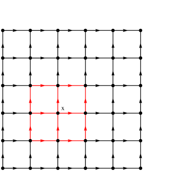
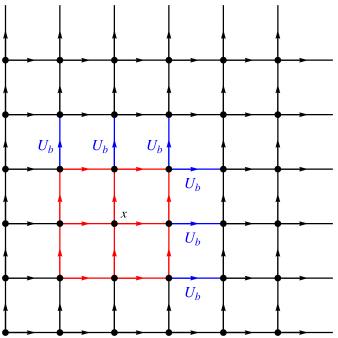
Figure 3: The lattice arrangement of gauge links for fixed “large” lattice ${\cal L}^{x}_{L}$ ($L\!=\!6$) and its “small” sublattice ${\cal L}^{x}_{\ell}$ ($\ell\!=\!3,r\!=\!1$) in case of open boundary conditions (left) and periodic boundary conditions in all directions (right).

To further exemplify the boundary approach, Fig. 3 illustrates two common situations. First, let the defining sequence of triples $({\cal L}^{x}_{L},S_{L},O_{x,L})$ be such that the prescription for action $S_{L}\!=\!S_{L}(U_{L})$ doesn’t involve any dangling links (left plot). This is the case of open boundary conditions and, since $\{\,U_{b}\,\}\!=\!\emptyset\,$, there is a single hypercubic boundary approximant $O_{x}^{r}(U)$ which is directly in covariant form. Secondly, assume that boundary conditions in $S_{L}\!=\!S_{L}(U_{L})$ are fully periodic in all directions (right plot). The subset of dangling links is now maximal as are the options for possible hypercubic boundary approximants. We emphasize that the sequence of triples $({\cal L}^{x}_{L},S_{L},O_{x,L})$ represents entire information apriori known about $O_{x}$. Given that, constructing covariant form $O_{x}^{r}(U)$ in periodic case can be viewed as extending the definition of $O_{x}(U)$ to the case with open boundary conditions.

3.1 Computational Efficiency

Important feature of the boundary approach is that it connects insensitivity to distant fields of an operator (and thus ultimately locality), to efficiency of its evaluation. More precisely, our main message in this regard is that insensitive operators generically have an efficient computer implementation provided by the boundary construction itself.

To formulate this, recall again that the operator $O_{x}(U)$ is defined via a sequence of triples $({\cal L}^{x}_{L},S_{L},O_{x,L})$, and is assumed to be computable in this section. This guarantees the existence of a program ${\cal P}$ that, given $\{L/a,U\}$, outputs $O_{x,L}$ to arbitrary accuracy. For simplicity, it is understood that the corresponding error is arranged to be much smaller than any other accuracy measure in the problem. In that sense

$${\cal P}\{L/a,U\}\,=\,O_{x,L}(U)$$ (34)

Note that we deal with a lattice situation and $a$ is not essential: with eventual continuum considerations in mind, we just chose to denote the parameter encoding the size of input field $U$ as $L/a$. Let ${\cal C}({\cal P},L/a,U)$ be the cost of running ${\cal P}\{L/a,U\}$ measured in required number of arithmetic operations. The average cost function for $O_{x}$ in realization ${\cal P}$ is then

$${\cal C}_{\cal P}(L/a)\,\equiv\,\bigl{\langle}\,{\cal C}({\cal P},L/a,U)\,\bigr{\rangle}_{S_{L}}$$ (35)

At the same time, the cost function of boundary approximant $O_{x}^{\ell}$ of Eq. (30) is

$${\cal C}_{\cal P}^{\prime}(\ell/a)\,\equiv\,\bigl{\langle}\,{\cal C}({\cal P},\ell/a,U_{\ell})\,\bigr{\rangle}_{S_{\ell}^{\prime}}$$ (36)

Here $S_{\ell}^{\prime}(U_{\ell})$ specifies the probability of fields $U_{\ell}$ on ${\cal L}^{x}_{\ell}$, arising when distribution of $U$ on ${\cal L}^{x}_{L}$ (given by $S_{L}(U)$) is marginalized via the $U\rightarrow U_{\ell}$ restriction. Thus, when replacing the operator with its boundary approximant, the cost of evaluating it via ${\cal P}$ changes as

$$O_{x}\;\longrightarrow\;O_{x}^{\ell}\qquad:\qquad\quad{\cal C}_{\cal P}(L/a)\;\longrightarrow\;{\cal C}_{\cal P}^{\prime}(\ell/a)$$ (37)

The situation is obviously analogous in case of hypercubic boundary approximants, except that $\ell\rightarrow\ell(r)$, and the action $S_{\ell(r)}^{\prime}=S_{\ell(r)}^{\prime}(U^{x,r})$ generally involves further marginalization due to the fixing of “boundary” $\{\,\bar{U}_{b}\,\}$. If $O_{x}$ is boundary insensitive, there exists hypercubic approximant $O_{x}^{r}$ and $\kappa\!>\!1$, $\mathscr{E}\!>\!0$ for which the bound (20) holds, and has $p\to 1$ limit with finite $R_{0}$ and ${\rho}_{0}(\kappa,\mathscr{E})$. The bound makes it possible to use the above default program ${\cal P}$ for computing $O_{x}(U)$ to arbitrary preset relative precision $\epsilon\!=\!\delta/\langle\|O_{x}\|\rangle$ without invoking the full volume. Indeed, it provides the minimal $r\!=\!{\cal R}_{\epsilon}$ for which $O_{x}^{r}(U)$ is guaranteed to produce error smaller than $\epsilon$, and we just feed ${\cal P}$ the input parameters $\ell({\cal R}_{\epsilon})$ and $U^{h}_{\ell({\cal R}_{\epsilon})}$. This running comes at the average computational cost

$${\cal C}_{\cal P}\left(\frac{L}{a}\right)\quad\longrightarrow\quad{\cal C}_{\cal P}^{\epsilon}\,\equiv\,{\cal C}_{\cal P}^{\prime}\left(\frac{\ell({\cal R}_{\epsilon})}{a}\right)\quad\;,\quad\;{\cal R}_{\epsilon}={\rho}_{0}+\max\left\{0,\,\kappa R_{0}\,\log\frac{\mathscr{E}}{\epsilon}\right\}$$ (38)

Note that ${\cal R}_{\epsilon}\!=\!{\rho}_{0}(\kappa,\mathscr{E})$ for all $\epsilon\!>\!\mathscr{E}$. In other words, $O_{x}^{{\rho}_{0}}$ is the “leading approximation”, with logarithmic dependence setting in for $\epsilon\leq\mathscr{E}$. There are several points to highlight.

(1) Formula (38) is universal in that it applies to arbitrary setup as described in Appendix D. Indeed, various situations only differ by the precise form of function $\ell(r)$.

(2) Using the boundary approximant in the above manner turns computation whose cost normally strongly depends on volume (l.h.s. of (38)) into one that involves a fixed-size input for given desired precision $\epsilon$, and is in that sense volume-independent. Importantly, this constant cost only depends logarithmically on $\epsilon$.

(3) Note that the formula (38) doesn’t assume anything about the nature of program ${\cal P}$. Indeed, starting from any valid ${\cal P}$, however inefficient, results in a volume-independent computation at fixed precision.

(4) It is clear that the cost functions ${\cal C}_{\cal P}(s)$ and ${\cal C}_{\cal P}^{\prime}(s)$ are not identical. However, their asymptotic behaviors ($s\rightarrow\infty$) are expected to be of the same type, with cost driven mainly by the number of field variables (input size) that have to be handled by the program as their abundance grows unbounded. Thus, if ${\cal C}_{\cal P}(s)$ grows exponentially or as a power, ${\cal C}_{\cal P}^{\prime}(s)$ generically grows in the same qualitative manner. Nevertheless, the introduction of boundary may affect the evaluation to the extent that the two cost functions are not simply asymptotically proportional. Taking the relevant case of power growth as an example, we can have

$${\cal C}_{\cal P}(s)\;\sim\;s^{d+\alpha}\qquad\qquad{\cal C}_{\cal P}^{\prime}(s)\;\sim\;s^{d+\alpha^{\prime}}\qquad\qquad s\rightarrow\infty$$ (39)

with possibly unequal $\alpha$, $\alpha^{\prime}$. For all standard ways of taking the infinite volume in zero-temperature calculations, function $\ell(r)$ is linear in $r$. For example, $\ell(r)\!=\!2r+a$ for maximally symmetric case (see Eq. (31)). With that, we have the asymptotic reduction

$$\left(\,\frac{L}{a}\,\right)^{d+\alpha}\;\xrightarrow[\scriptstyle\epsilon\to 0]{\qquad}\quad\left(\,\frac{\ell({\cal R}_{\epsilon})}{a}\,\right)^{d+\alpha^{\prime}}\quad\sim\quad\left(\,\frac{R_{0}}{a}\,\log\frac{\mathscr{E}}{\epsilon}\,\right)^{d+\alpha^{\prime}}\quad,\quad\alpha,\alpha^{\prime}\geq-d$$ (3’)

which is a generalized version of (3) in the relative error form. Note that $\alpha\!=\!\alpha^{\prime}\!=\!-d$ for ultralocal operator since the cost is constant, and one generically expects $\alpha\geq 0$ for non-ultralocal operator coupled to all field variables, such as $D_{x,x}(U)$ of overlap Dirac matrix.

(6) If the choice of input for program ${\cal P}$ was based on parameters at given statistical cutoff $p$, i.e. $R_{0}(p)$, ${\rho}_{0}(\kappa,\mathscr{E},p)$, the result of any particular run would be good to relative precision $\epsilon$ with probability at least $p$. This in itself is a powerful advantage of even weakly insensitive non-ultralocal operators, where $p$ can be set arbitrarily close to unity.

4 Overlap-Based Gauge Operators

In what follows, we apply the framework developed in Secs. 2,3 to study boundary insensitivity and locality properties of the operator

$$O_{x}(U)\,\equiv\,D_{x,x}(U)-D_{x,x}^{F}$$ (40)

where $D(U)$ is the overlap color-spin matrix and $D^{F}$ its free subtraction ($U_{y,\mu}\to\mathbf{1}$). Its relevance is that useful operators of practical interest such as topological density $q(x)$, scalar gauge density $s(x)$ and field-strength tensor $F_{\mu\nu}(x)$ are based on it, namely

$$q(x)\,\propto\,\mathop{\rm Tr}\gamma_{5}O_{x}\qquad\qquad s(x)\,\propto\,\mathop{\rm Tr}O_{x}\qquad\qquad F_{\mu\nu}(x)\,\propto\,{\mathop{\rm Tr}}_{s}\,\sigma_{\mu\nu}O_{x}$$ (41)

where $\mathop{\rm Tr}_{s}$ denotes the trace over spin indices only. Note that the free subtraction in $O_{x}$ is consequential for scalar density but not for the other two operators.

It should be remarked here that the obvious role of the above $O_{x}(U)$ as a master construct in definitions (41) is further underlined by the fact that its potential insensitivity at fixed $p$ and $a$ descends onto these derived operators of interest. This can be seen from the fact that the Frobenius matrix norm $\|M\|^{2}\equiv\mathop{\rm Tr}(M^{+}M)$, which we will use to quantify the differences of matrix-valued operators and define the error functions $\delta(r,p)$, is sub-multiplicative, i.e. $\|M_{1}M_{2}\|\leq\|M_{1}\|\|M_{2}\|$. Thus, the requisite exponential bounds for $O_{x}(U)$ can be used to produce the associated (albeit non-optimal) bounds for derived operators. Nevertheless, the concrete behavior of optimal bounds for individual operators is of practical interest since their precise form guides the efficient evaluation of these operators. In particular, the threshold distances ${\rho}_{0}$ could vary appreciably among them.

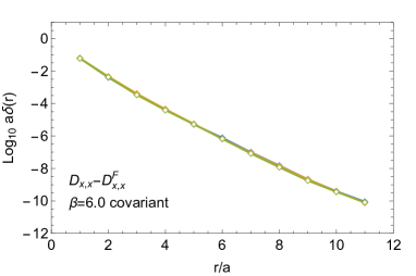
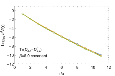
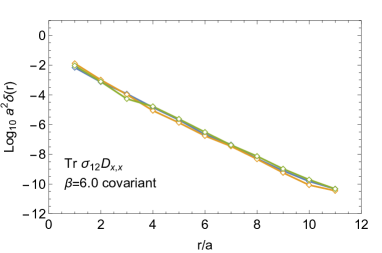
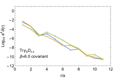
Figure 4: The behavior of $\delta(r)$ for covariant boundary approximant at three randomly chosen individual points at $\beta\!=\!6.0$.

4.1 The Setup

For our numerical work, we use the symmetric $L^{4}$ lattice geometry adopted as a template for the general discussion of Secs. 2,3. The insensitivity and locality of the above overlap-based gauge operators will be studied with respect to to pure-glue SU(3) theory with Wilson gauge action, and periodic boundary conditions for gauge fields in all directions.

The overlap Dirac operator in (40) is based on the Wilson-Dirac kernel and the parameter $\rho\in(0,2)$, specifying its negative mass, set to $\rho\!=\!1.368$ ($\kappa\!=\!0.19$). Definition of the operator is given in Appendix E. Standard boundary conditions for quarks, i.e. periodic in “space” and antiperiodic in “time”, are used although there is no fundamental preference in that regard. In fact, when the sole purpose of utilizing the overlap is to define gauge operators, one may opt for periodic boundaries in all directions to maximize hypercubic symmetries. The resulting $D_{x,x}(U)$ is gauge covariant and periodic in all directions.

With regard to the computational realization of the overlap, we follow the MinMax polynomial approach of Ref. [14] in a specific implementation discussed in Ref. [15]. Using deflation as needed, we explicitly ensured that the accuracy in evaluation of the overlap is always significantly better than any quoted error of a boundary approximant. In other words, in what follows, Eq. (34) can be assumed to be valid without further qualifications.

To study the insensitivity and locality properties of the above operators, we generated three ensembles of $L/a\!=\!24$ configurations at $\beta\!=\!6.0,6.2,6.4$. This corresponds to nominal lattice spacings of $a\!=\!0.093,0.068,0.051\,$fm respectively, based on $r_{0}\!=\!0.5$ fm. While the finest ($\beta\!=\!6.4$) lattice system is clearly quite squeezed in physical terms, this is of little consequence for the current study. Indeed, as the discussion later in this paper reveals, the finite volume effects on observables of our interest are negligible.

As expected on general grounds, the default hypercubic boundary approximant $O_{x}^{r}$ (covariant one) is well-defined, and can be computed straightforwardly by running the program designed to evaluate $O_{x}$ on input that corresponds to the boundary subsystem. For 20 configurations from each of the above ensembles, we computed $O_{x}$ as well as its approximants $O_{x}^{r}$ for all possible distances $r$, at 16 points evenly distributed on the lattice. Note that this calculation produces estimates for all derived operators (41).

To obtain a preliminary assessment of boundary approximants, we plot in Fig. 4 the dependence of error ${\delta}$ on hypercubic radius $r$ at three randomly chosen points $x$ in a given $\beta\!=\!6.0$ configuration. As can be seen quite clearly, a straightforward exponential-like decay takes place even on an individual point basis. The behavior is least orderly in case of pseudoscalar density (bottom right), but the overall trend is quite unmistakable in that case as well. A systematic investigation using statistical regularization is thus warranted.

4.2 Finite Volume

As emphasized in Sec. 2 (see Definition 1), exponential insensitivity is an infinite-volume concept. In particular, the property depends on the behavior of statistically regularized error function in asymptotically large volumes, i.e. $\delta(r,p)\!=\!\lim_{L\to\infty}\delta(r,p,L)$. However, in practice, we are bound to infer the exponential behavior from a sequence of finite, and usually limited volumes. To ensure that such estimates are reliable, it needs to be checked that $\delta(r,p,L)$ is insensitive to $L$ over the range of distances $r$ used in such calculations.

       

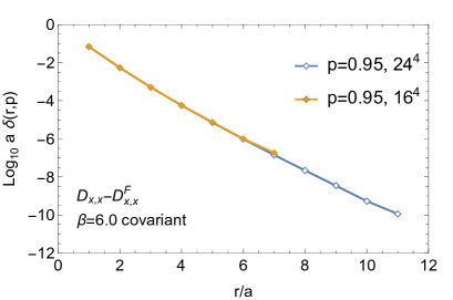
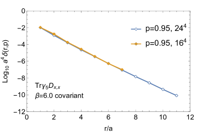
Figure 5: The volume comparison at $p\!=\!0.95$ for $O_{x}$ (left) and $\mathop{\rm Tr}\gamma_{5}O_{x}$ (right).

To examine this issue, we supplemented the $\beta\!=\!6.0$ ensemble at $L/a\!=\!24$ with one at $L/a\!=\!16$. Notice that, since $\ell(r)\!=\!2r+a$, the maximal hypercubic radius for given $L/a$ is $r_{m}/a\!=\!\mathop{\rm floor}(L/2a)$, i.e. $r_{m}\!=\!11a$ and $r_{m}\!=\!7a$ correspondingly. In Fig. 5 we compare the results on the two volumes for $O_{x}$ and the pseudoscalar density at $p\!=\!0.95$. The behavior for other operators is completely analogous. It is quite obvious that we have an excellent agreement over the range of common radii. Close to $r\!=\!r_{m}$ one expects some edge effects in principle and, to avoid the possibility of such contamination, we only extract the parameters of exponential behavior from distances up to $r\!=\!r_{m}\!-\!a$ in what follows.

4.3 Insensitivity and Weak Locality

The results of the volume study show that error functions of hypercubic boundary approximants at $p\!=\!0.95$ are exponentially boundable. Recalling the more complete results of Fig. 2, including other operators and the range of cutoffs $p$, it is quite obvious that overlap-based gauge operators are insensitive at any fixed $p\!<\!1$. Thus, within the classification of Sec. 2, they are weakly insensitive lattice operators at the ultraviolet cutoff in question ($\beta\!=\!6.0$). Results completely analogous to those of Fig. 2 were found also for the other two ensembles representing finer lattices. The question then arises whether continuum operators $O_{x}^{c}$ defined by their overlap-based constructions are themselves weakly insensitive or insensitive. This requires demonstrating the insensitivity of $O_{x}^{c}$ at any fixed $p$ (see Definition 3).

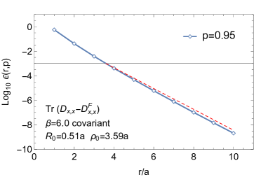
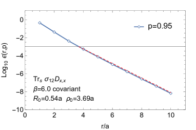
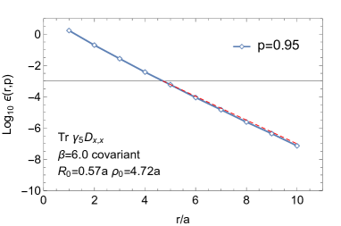
Figure 6: The behavior of $\epsilon(r)$ for covariant boundary approximant at $p\!=\!0.95$ and $\beta\!=\!6.0$. The optimal exponential bounds are shown at $\kappa\!=\!1$ and $\mathscr{E}\!=\!10^{-3}$, indicating the thresholds.

To undertake this, the relative error data has to be characterized in terms of the corresponding bound parameters, as described in Sec. 2.5. In particular, we need to monitor the scales $R_{0}(p,a)$ and ${\rho}_{0}(\kappa,\mathscr{E},p,a)$ associated with $\epsilon(r,p,a)$ (see Eq. (26)) at arbitrary but fixed $\kappa\!>\!1$ and $\mathscr{E}\!>\!0$. As seen from the representative data shown already, $R_{0}(p,a)$ can be estimated by simply fitting the measured error functions to exponentials at large distances. In what follows, we extract these effective ranges using the three largest radii smaller than $r_{m}$. Our analysis of the available data does not support the presence of unbounded modulation in asymptotically exponential decays of $\epsilon(r)$. Consequently we can, and always do, determine ${\rho}_{0}$ at $\kappa\!=\!1$. While the threshold error $\mathscr{E}$ can be set to arbitrary positive value, we use $\mathscr{E}\!=\!10^{-3}$ here, i.e. the absolute error at ${\rho}_{0}$ is one part in a thousand of the average operator magnitude. The associated bound then describes the errors for $r\!>\!{\rho}_{0}$ quite faithfully and can be used to predict the needed hypercubic radii in practical calculations. The situation for all operators of interest at statistical cutoff $p\!=\!0.95$ is shown in Fig. 6.

We are now equipped to examine the removal of ultraviolet cutoff at fixed $p$. Fig. 7 conveys the relevant data for $O_{x}$ and topological density. In particular, the top row shows $\epsilon(r,p\!=\!0.95)$ as a function of physical distance at all three ultraviolet cutoffs. The effect of gauge fields beyond fixed distance $r$ clearly decays very rapidly and there is thus no doubt that the parameters of the corresponding exponential bounds $R_{0}(p\!=\!0.95,a)$ and ${\rho}_{0}(p\!=\!0.95,a)$ are decreasing functions of $a$, and can only have finite continuum limits $R_{0}^{c}(p\!=\!0.95)$, ${\rho}_{0}^{c}(p\!=\!0.95)$. This behavior is readily present at all cutoffs $p$ accessible by our statistics, and we conclude that the corresponding continuum operators are weakly insensitive.

Making more restrictive conclusions about insensitivity, or assessing locality, requires cutoff-monitoring of the bound parameters. The bottom row of Fig. 7 shows their dependence on ultraviolet cutoff. With constant fits for $R_{0}/a$ and linear fits for ${\rho}_{0}/a$ added to guide the eye, our data conveys quite clearly that finite extrapolations in lattice units exist in both cases. This behavior is generic in $p$ and we conclude that

$$R_{0}(p,a)\propto a\qquad\quad{\rho}_{0}(p,a)\propto a\quad\;,\quad\;\forall\,p<1$$ (42)

for all operators in question. It follows that $R_{0}^{c}(p)$ and ${\rho}_{0}^{c}(p)$ are zero, which in turn implies that their $p\!\to\!1$ limits $R_{0}^{c}$ and ${\rho}_{0}^{c}$ vanish as well. In other words, the continuum gauge operators based on the overlap are exponentially insensitive to distant fields (Definition 4) and weakly local (Definition 6).

   

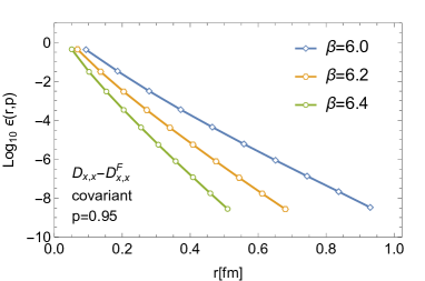
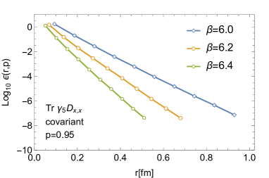
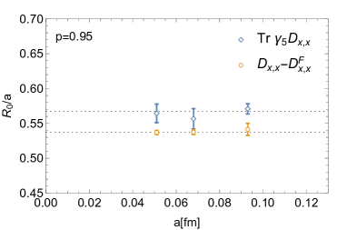
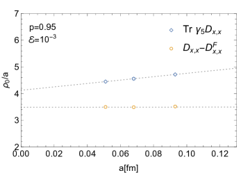
Figure 7: The behavior of $\epsilon(r,p\!=\!0.95)$ at different ultraviolet cutoffs (top) and the lattice spacing dependence of exponential bound parameters (bottom). Discussion is in the text.

4.4 Strong Insensitivity and Locality

In the formalism we adopted, weak insensitivity of defining lattice operators (sufficiently close to the continuum limit) constitutes a necessary precursor to insensitivity and weak locality in the continuum. Indeed, these concepts feature the order $\lim_{p\to 1}\lim_{a\to 0}$ in the removal of cutoffs. As discussed in the previous section, our analysis indicates that both of these properties in fact materialize in the overlap-based gauge operators.

In a similar manner, insensitivity of lattice operators (Definition 2) is a necessary precursor to continuum notions of strong insensitivity and locality, since the reverse order $\lim_{a\to 0}\lim_{p\to 1}$ of taking limits applies. Note that establishing strict lattice insensitivity can be a demanding task. Indeed, here the question whether potential outliers of a given bound form a set of measure zero enters most directly, and it is thus crucial that the statistics be sufficient to capture the nature of parameter behavior in the vicinity of $p\!=\!1$.

   

   

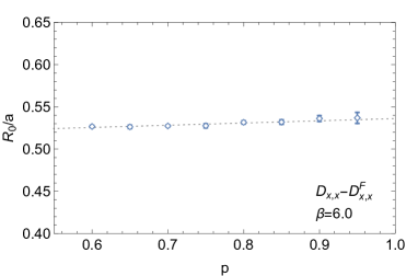
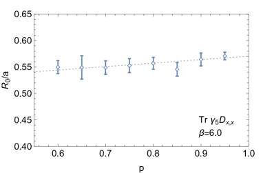
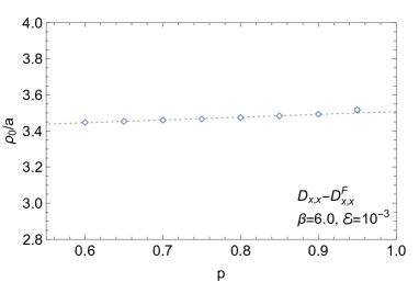
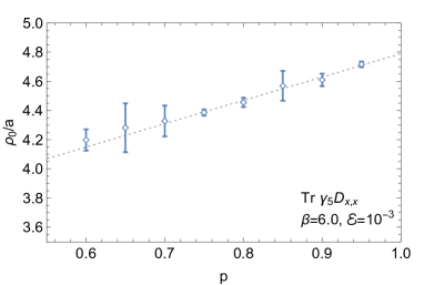
Figure 8: The $p$-dependence of exponential bound parameters for $O_{x}$ (left column) and $q(x)$ (right column) at $\beta\!=\!6.0$. See the discussion in the text.

While our statistics is rather limited in this regard, the look at the available data is revealing. In Fig. 8 we show the $p$-dependence of $R_{0}$ and ${\rho}_{0}$ in lattice units at $\beta\!=\!6.0$ for $O_{x}$ and topological density. First, one should realize that it follows from definitions of both $R_{0}$ and ${\rho}_{0}$ that they are non-decreasing functions of $p$. In case of $R_{0}$ we only observe an extremely mild trend in this regard, well described by the linear behavior fitted to guide the eye. The situation is similar for ${\rho}_{0}$, albeit the rise in case of topological density is visibly steeper than for $O_{x}$.

Assuming that the observed trends do not change dramatically closer to $p\!=\!1$, the above would suggest that finite $p\!\to\!1$ limits of parameters exists and, consequently, that the overlap-based gauge operators are exponentially insensitive at the lattice level. With that, the issues of strong insensitivity/locality in the continuum would become well-posed, and the corresponding tendencies to obtain $\bar{R}_{0}$ and $\bar{{\rho}}_{0}$ in lattice units shown in Fig. 9 (top) for topological density. Finite extrapolations to continuum limit are then readily concluded from the data, implying both of the above continuum properties.

   

   

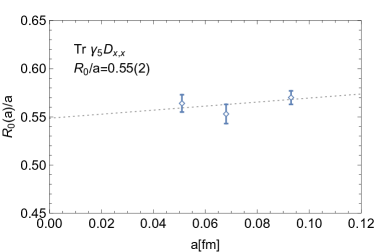
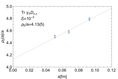
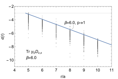
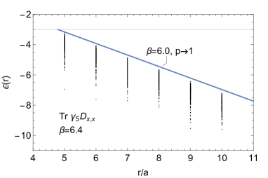
Figure 9: Top: continuum extrapolation to determine $\bar{R}_{0}/a$ and $\bar{{\rho}}_{0}/a$ (topological density). Bottom: $p\!\to\!1$ bound at $\beta\!=\!6.0$ (left) and the same bound with data at $\beta\!=\!6.4$ (right).

However, the assumption about the behavior closer to $p\!\to\!1$ does need to be scrutinized. Indeed, our statistics allows for reliable extraction of bound parameters up to $p\!=\!0.95$, but the fluctuations in error do become somewhat larger for the “outliers”. Indeed, in Fig. 9 (bottom, left) we show the $p\!\to\!1$ extrapolated bound at $\beta\!=\!6.0$ together with actual samples of approximation differences. While the bound at $p\!=\!0.95$ would leave out 16 outliers at each $r/a$, the extrapolated bound still leaves out about 4 on average, almost certainly pushing a small residual probability outside its reach. This suggests that the behavior of bound parameters is somewhat modified in the immediate vicinity of $p\!=\!1$ at $\beta\!=\!6.0$, and significantly larger statistics needs to be invoked to extrapolate reliably.

Nevertheless, even with the current data, one can make the existence of $p$-independent bound sufficiently close to the continuum limit quite plausible. Indeed, if $R_{0}(a_{0})$, ${\rho}_{0}(a_{0})$ are the $p\!\to\!1$ extrapolated bound parameters at lattice spacing $a_{0}$, let $R(a)\!=\!aR_{0}(a_{0})/a_{0}$ and ${\rho}(a)\!=\!a{\rho}_{0}(a_{0})/a_{0}$ be the parameters of a (non-optimal) bound at lattice spacing $a\!<\!a_{0}$. Thus, in lattice units, this bound is the same for all $a\!\leq\!a_{0}$. Due to the observed decreasing trend of ${\rho}_{0}(a)/a$ for $a\!\to\!0$ (top right in Fig. 9) such bound may become $p$-independent sufficiently close to the continuum limit. Associating $a_{0}$ with $\beta\!=\!6.0$ ensemble, in Fig. 9 (bottom, right) we show the relation of errors at $\beta\!=\!6.4$ to this bound and, indeed, there are no violations at our level of statistics. Needless to say though, the issue of strong insensitivity and locality in overlap-based continuum operators needs to be resolved via a direct extensive calculation.

5 Application: Topological Structure in QCD Vacuum

The computational aspect of insensitivity considerations becomes relevant in practice when the problem at hand significantly benefits from the use of non-ultralocal operators. One example is the study of QCD vacuum structure via overlap-based topological charge density $q(x)$. This stems from the fact that $q(x)$ is topological, i.e. stable under deformations of the gauge field, directly on the lattice. Indeed, this property was instrumental in finding that, when fluctuations at all scales are included, topological charge in QCD organizes into low-dimensional global structure of space-filling type [12]. The structure takes the form of a double sheet formed by topological densities of opposite sign, and is inherently global [16]. In particular, this space-spanning object cannot be broken into individual pieces without severely affecting topological susceptibility.

Computational issue hampering extensive investigations of the above type is that, since $q(x)$ needs to be evaluated on entire lattices, the use of standard overlap implementations leads to costs that scale at least as $V^{2}$. As we argued extensively, utilizing hypercubic boundary approximants effectively turns this into a generic $V$-problem with pre-factor depending only logarithmically on the desired precision. One should realize in this regard that, while boundary insensitivity guarantees eventual fast convergence in the radius of the approximant, the sufficiency criteria for this radius are problem-specific. For example, if the goal were to reliably determine the space-time structure in the sign of topological charge (see Ref. [17]), then the relevant criterion would be a sufficiently low rate of sign violations in the approximant. In Fig. 10 (left) we show such data for ensemble at $\beta\!=\!6.0$. Within the available statistics, no violations are observed already at $r\!=\!3a$. More quantitatively, the rate of violation can be estimated to be significantly better than 1% at $r\!=\!3a$, and is likely negligible for all practical purposes at $r\!=\!4a$, providing for a safe choice to fix when working at arbitrarily large volume.

       

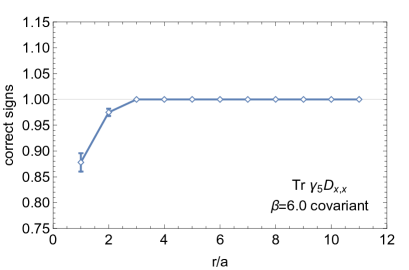
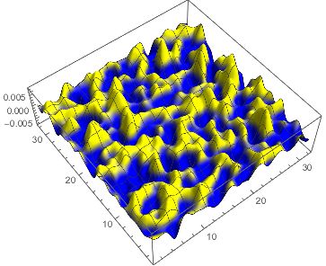
Figure 10: Left: the rate of correct sign when approximating topological density by covariant boundary approximant at $\beta\!=\!6.0$. Right: typical 2d slice through global topological structure on $32^{4}$ system, computed via boundary approximant with $r\!=\!6a$.

If the goal is to gain more detailed information on the topological structure, we can use the values of bound parameters at various statistical cutoffs $p$ to obtain needed estimates. Alternatively, one can again examine the criterion in question as a function of hypercubic radius $r$ in a preliminary study. In the context of topological charge, a suitable generic requirement is that its global integer value be reproduced to a prescribed accuracy in the approximation. To gain some quantitative feel on this and other aspects, we have computed configurations of topological charge at various couplings in pure-glue lattice gauge theory with Iwasaki gauge action. While the analysis of these results will be given elsewhere, here we point out that these computations for $24^{4}$ system at $a\!=\!0.055\,$fm yield the typical absolute error of $10^{-3}$ for global charge using $r\!=\!5a$ boundary approximant. The situation is quantitatively similar for $32^{4}$ system at $a\!=\!0.041\,$fm (same physical volume) using $r\!=\!6a$ approximant. The typical profile of topological structure on 2d slice of space-time is shown in Fig. 10 (right). The properties of the structure conform to those concluded in Ref. [12].

6 Summary and Conclusions

Locality is an important ingredient and guiding principle in describing natural phenomena via quantum fields. In this paper we reexamined this notion in the context of Euclidean field theories, such as Euclidean QCD, with quantum continuum dynamics defined via lattice-regularized path integral. While the approach is entirely general with respect to the fundamental field content, our discussion was carried out for operators composed of gauge fields. This is partially motivated by the fact that locality properties for useful non-ultralocal gauge operators have not been previously studied.

Locality is a strictly continuum notion: it is a property of continuum object $O_{x}^{c}(A)$, operationally defined via certain lattice $O_{x}(U)$ in the limiting process of driving the theory to the continuum limit. However, there is a more general concept, meaningful already on the lattice, that ushers locality into the continuum as its special case. Indeed, universality arguments suggest that such lattice precursor of locality is the exponentially weak dependence of $O_{x}(U)$ on fields residing sufficiently far from $x$. One of the main results in this paper is a novel formulation of this exponential insensitivity to distant fields.

Our approach to insensitivity is information-like in that it probes how well is it possible to know $O_{x}(U)$ when $U$ itself is only known in the neighborhood of $x$ with radius $r$, i.e. when only the patch $U^{x,r}\!\subset\!U$ of the gauge field is accessible. This can be quantified by the accuracy achievable by the approximants $O_{x}(U)\rightarrow O_{x}^{r}(U)\!=\!O_{x}^{r}(U^{x,r})$ enforcing this restriction. Exponential insensitivity to distant fields is then the ability to construct the sequence $O_{x}^{r}$ whose accuracy can be bounded by a decaying exponential in $r$.

Making this idea precise requires us to specify the measure for “accuracy” of a given approximant, with subtlety being that there is, in fact, a distribution of errors generated by the underlying path integral distribution of gauge fields for the theory in question. To have a tunable control over the scope of these deviations, and to accommodate cases where violations of exponential bound form a probabilistic set of measure zero, we introduce the procedure of statistical regularization. Here boundability relates to the fraction $p$ of the path integral population with smallest errors, which amounts to the concept of least upper bound with probability $p$. At every statistical cutoff $p$, the problem of exponential boundability is well-posed, and the general framework describing degrees of exponential insensitivity in the process of statistical ($p\!\to\!1$) and ultraviolet ($a\!\to\!0$) cutoff removals ensues. Locality, then, is simply associated with vanishing of scales describing the cutoff-removed bounds.

Classification of composite operators by degree of exponential insensitivity can in principle proceed by examining the properties of their optimal approximant [13]. However, in the realm of computable operators, the evaluation of this $O_{x}^{r,op}(U^{x,r})$ is much more expensive than that of $O_{x}(U)$ alone, except for simple ultralocal cases. At the same time, constructing any approximant with required properties demonstrates insensitivity. This motivates our proposal to consider boundary approximants, wherein the value $O_{x,L}(U)$ on the “large” system of size $L$, is replaced by the value $O_{x,2r+a}(U^{x,r})$ on the “small” system spanned by the hypercubic field patch alone. Such approximant probes insensitivity to distant fields by inserting an artificial boundary distance $r$ away from $x$, giving rise to a somewhat stronger, but physically well-motivated notion of boundary insensitivity and boundary locality.

Determining boundary insensitivity is a straightforward task for any computable $O_{x}(U)$. Moreover, if there is a program evaluating $O_{x,L}(U)$ with polynomial complexity in $L/a$ (typical case), then the property of boundary insensitivity makes it possible for $O_{x,L}(U)$ to be computed efficiently. Indeed, running the same program on input corresponding to boundary subsystem affording the desired accuracy $\epsilon$, results in volume-independent computation whose cost only grows as a power of $\log 1/\epsilon$. This connection between efficient computation and exponential insensitivity/locality is one of the main conceptual points emphasized in this paper. Its full scope and ramifications will be explored elsewhere.

1. The boundary insensitivity analysis was applied to gauge operators based on the overlap Dirac matrix, such as topological charge density or field-strength tensor. Apart from illustrating the general scheme, our goal was to examine locality properties of these useful non-ultralocal operators on realistic equilibrium backgrounds. Invoking the hierarchy developed here, our results clearly indicate that these operators are weakly insensitive at the lattice level, and weakly local in the continuum. Quantitative evidence has also been presented favoring insensitivity on the lattice, and locality in the continuum. However, putting these latter findings on a firm ground requires more extensive simulations to be performed. Overall, our analysis shows that there is little doubt that these operators follow the universal behavior in the continuum.

2. Important practical outcome of our numerical experiments with boundary approximants is that their power of exponential improvement in estimating $O_{x}(U)$ pans out already at small values of hypercubic radii. Our experience with overlap-based topological density in particular, suggests that using this technique makes extensive vacuum structure studies with such complicated operator no longer computationally prohibitive.

3. For fixed $r/a$, the approximant $O_{x}^{r}$, facilitating the insensitivity of $O_{x}$, is simply an ultralocal lattice operator that could be interesting in its own right. In case of gauge operators studied here, the covariant form of boundary $O_{x}^{r}$ (default choice) inherits all potential symmetries of $O_{x}$, making it a particularly attractive choice for standalone use.

4. The exponential insensitivity framework can be viewed as a tool to classify all lattice-defined continuum operators $O_{x}^{c}$ in terms of their reach. This is quantified by the characteristic length scales introduced, such as the range $R_{0}^{c}$ and threshold ${\rho}_{0}^{c}$. We expect such description to be useful for defining non-local operators at fixed scale.

Acknowledgments: We thank Thomas Streuer for participating in the early stages of this project. A.A. is supported in part by the National Science Foundation CAREER grant PHY-1151648 and Department of Energy grant DE-FG02-95ER40907. I.H. acknowledges the support by Department of Anesthesiology at the University of Kentucky.

Appendix A Regularity of the Approximation

The notion of exponential insensitivity aims at capturing the exponential (in distance) control over values of the composite operator. Such concept would be unsatisfactory if it admitted cases wherein the zero-measure sample set of violations contributed finitely to the statistics of $O_{x}$. To prevent such singular behaviors from being considered insensitive, we formulate here the corresponding requirement of regularity.

Strictly speaking, regularity needs to be examined in conjunction with any statistical inference wherein $O_{x}$ is replaced by its approximant $O_{x}^{r}$. Relevant situations may also involve arbitrary other operators but, as a defining property, it relates to $O_{x}$ itself. Thus, in addition to the error function ${\delta}(r,p,a)$, function ${\cal A}(r,p,a)$ is defined as a contribution to mean magnitude of $O_{x}$ due to samples whose error is larger than ${\delta}(r,p,a)$, i.e. due to “violations” at statistical cutoff $p$. If $\bar{\cal A}(r,p,a)$ is the portion governed by cutoff $p$, then

$$\langle\,\|O_{x}\|\,\rangle_{a}\,=\,\bar{\cal A}(r,p,a)\,+\,{\cal A}(r,p,a)$$ (43)

In the same way, let ${\cal A}_{\tt ap}(r,p,a)$ be the part of $\langle\,\|O_{x}^{r}\|\,\rangle_{a}$ due to violations. Approximation $O_{x}^{r}$ of lattice operator $O_{x}$ at fixed ultraviolet cutoff $a$ is regular if there exists $r_{0}$ such that

$$\lim_{p\to 1}{\cal A}(r,p,a)\,=\,0\qquad\qquad\lim_{p\to 1}{\cal A}_{\tt ap}(r,p,a)\,=\,0\qquad,\qquad\forall\,r\geq r_{0}$$ (44)

While the first condition ensures that excluding the zero-measure set of violations doesn’t lead to finite distortion, the second one ascertains that replacing it with zero-measure set of approximants doesn’t do that either. Regularity of the approximation is required for lattice operator $O_{x}$ to be weakly insensitive.

Additional care needs to be taken when examining exponential insensitivity in the continuum (Definition 4). Here $a\!\to\!0$ limit is taken at fixed $p$ first, which may lead to a finite influence in subsequent $p\!\to\!1$ limit even when lattice operator is regularly approximated at any $a$. Moreover, the contribution of outliers has to be considered relative to $a$-dependent average magnitude. In particular, the continuum regularity condition reads

$$\lim_{p\to 1}\lim_{a\to 0}\,\frac{{\cal A}(r,p,a)}{\langle\,\|O_{x}\|\,\rangle_{a}}\,=\,\lim_{p\to 1}\lim_{a\to 0}\,\frac{{\cal A}_{\tt ap}(r,p,a)}{\langle\,\|O_{x}\|\,\rangle_{a}}\,=\,0\qquad,\qquad\forall\,r\geq r_{0}$$ (45)

It is worth noting that, while lattice regularity (44) is automatically satisfied for bounded pair $O_{x}$ and $O_{x}^{r}$, lattice boundedness at any $a$ does not necessarily guarantee (45).

Appendix B Parametric Freedom in Statistical Cutoff Removal

This Appendix elaborates on point (i) of discussion in Sec. 2.4. In particular, we first aim to show that if ${\rho}_{0}(\kappa,\mathscr{E})\!<\!\infty$, then ${\rho}_{0}(\kappa,\mathscr{E}^{\prime})\!<\!\infty$ for all $\mathscr{E}^{\prime}>0$. More explicitly

$$\lim_{p\to 1}{\rho}_{0}(\kappa,\mathscr{E},p)<\infty\quad\Longrightarrow\quad\lim_{p\to 1}{\rho}_{0}(\kappa,\mathscr{E}^{\prime},p)<\infty\quad,\quad\forall\;\mathscr{E}^{\prime}>0$$ (46)

Before proceeding, it is useful to summarize the monotonicity properties of ${\rho}_{0}(\kappa,\mathscr{E},p)$. From Eqs. (10,12,13,19) it follows that ${\rho}_{0}(\kappa,\mathscr{E},p)$ is decreasing in $\mathscr{E}$ and non-increasing in $\kappa$. Moreover, since ${\delta}(r,p)$ is non-decreasing in $p$, so is $\Delta_{0}(R,{\rho},p)$, and consequently ${\rho}_{0}(\kappa,\mathscr{E},p)$.

To show (46), first assume that $\mathscr{E}^{\prime}\!>\!\mathscr{E}$, implying that ${\rho}_{0}(\kappa,\mathscr{E}^{\prime},p)\!<\!{\rho}_{0}(\kappa,\mathscr{E},p)$, $\forall\,p\!<\!1$. Given that ${\rho}_{0}$ is non-decreasing in $p$, the existence of $p\!\to\!1$ limit on the right side of this inequality implies the existence of the limit on the left side, as claimed by (46). To include the case $\mathscr{E}^{\prime}\!<\!\mathscr{E}$, first note that ${\rho}_{0}(\kappa,\mathscr{E},p)$ is a solution of the equation

$$\Delta_{0}(R,{\rho}_{0},p)\,\equiv\,B(R,{\rho}_{0},p)\exp\Bigl{(}-\frac{{\rho}_{0}}{R}\Bigr{)}\;=\;\mathscr{E}\,\langle\|O_{x}\|\rangle\qquad\text{with}\qquad R=\kappa R_{0}(p)$$ (47)

Combining this with the analogous equation for $\mathscr{E}^{\prime}$ and taking into account that function $B(R,{\rho}_{0},p)$ is non-increasing in ${\rho}_{0}$ while ${\rho}_{0}$ is itself decreasing in $\mathscr{E}$, we obtain the inequality

$${\rho}_{0}(\kappa,\mathscr{E}^{\prime},p)\,\leq\,{\rho}_{0}(\kappa,\mathscr{E},p)\,+\,\kappa R_{0}(p)\log\frac{\mathscr{E}}{\mathscr{E}^{\prime}}\qquad,\qquad\mathscr{E}^{\prime}<\mathscr{E}$$ (48)

Since ${\rho}_{0}$ is non-decreasing in $p$, and a finite $p\!\to\!1$ limit on the right side of this inequality exists, the finite limit also exists on the left side, demonstrating (46).

The second claim we aim to substantiate here is that ${\rho}_{0}(\kappa,\mathscr{E})\!<\!\infty$ implies ${\rho}_{0}(\kappa^{\prime},\mathscr{E})\!<\!\infty$ for $\kappa^{\prime}>\kappa$, but not for $1\!<\!\kappa^{\prime}\!<\!\kappa$. The former follows from monotonicity properties of ${\rho}_{0}$ in a manner analogous to that discussed in case of $\mathscr{E}$. To show the latter, it suffices to construct a possible ${\delta}(r,p)$ that exemplifies the corresponding behavior. One option is

$${\delta}(r,p)=\text{Taylor}\biggl{[}\,\exp\Bigl{(}\frac{r}{2R_{1}}\Bigr{)}\,,\,\mathop{\rm floor}\biggl{(}\frac{1}{1-p}\biggr{)}\,\biggr{]}\;\exp\Bigl{(}-\frac{r}{R_{1}}\Bigr{)}$$ (49)

where $R_{1}$ is a constant and $\text{Taylor}(f(x),n)$ the Taylor series of $f(x)$ around $x\!=\!0$ up to $n$-th order. Clearly, $\lim_{p\to 1}R_{0}(p)=\lim_{p\to 1}R_{1}=R_{1}$ and, due to the chosen $p$-deformation of the prefactor, finite ${\rho}_{0}(\kappa,\mathscr{E})$ is only obtained via $\kappa R_{0}(p)\!\geq\!2R_{1}$, i.e. with $\kappa\!\geq\!2$.

Appendix C More on the Ultraviolet Cutoff Removal

Here we elaborate on the most general form of Definition 3, specifying exponential insensitivity at fixed $p$ in the continuum, i.e. on the procedure of ultraviolet cutoff removal. This generalization requires the existence of $O_{x}^{r}$, $a_{0}\!>\!0$, $\kappa\!>\!1$ and $\mathscr{E}\!>\!0$ such that

$$\sup\,\{\,R_{0}(p,a)\,\mid\,0\!<\!a\!<\!a_{0}\,\}<\infty\qquad\ \qquad\sup\,\{\,{\rho}_{0}(\kappa,\mathscr{E},p,a)\,\mid\,0\!<\!a\!<\!a_{0}\,\}<\infty$$ (50)

Clearly, when $O_{x}(U)$ satisfies Definition 3 at given $p$, it also satisfies the above, but not vice versa. Indeed, it is possible to construct functions satisfying bounds (50), for which $a\!\to\!0$ limits (22) do not exist. While such $a$-dependences are not likely to occur for operators of practical interest, specifying a complete framework for characterizing exponential insensitivity to distant fields is clearly of conceptual interest at the very least.

The question that remains to be answered in this regard is how to assign the continuum effective range and the threshold distance to operator-approximant combinations that behave in such non-standard way. Indeed, in cases covered by Definition 3, these are the scales $R_{0}^{c}(p)$ and ${\rho}_{0}(\kappa,\mathscr{E},p)$ specified by the limiting procedure which is ill-defined in this situation. For the appropriate generalization, we denote the bounds (suprema) of (50) as $R_{b}(p,a_{0})$ and ${\rho}_{b}(\kappa,\mathscr{E},p,a_{0})$ respectively, and define

$$R_{b}^{c}(p)\,\equiv\,\lim_{a_{0}\to 0}\,R_{b}(p,a_{0})\qquad\qquad{\rho}_{b}^{c}(\kappa,\mathscr{E},p)\,\equiv\,\lim_{a_{0}\to 0}\,{\rho}_{b}(\kappa,\mathscr{E},p,a_{0})$$ (51)

Note that, since $R_{b}(p,a_{0})$ and ${\rho}_{b}(\kappa,\mathscr{E},p,a_{0})$ are non-decreasing in $a_{0}$, the existence of these limits is guaranteed by (50). Clearly, the meaning of these characteristics is that they specify the optimal exponential bounds (20) in the continuum.

Finally, we point out that the finiteness of ${\rho}_{b}^{c}(\kappa,\mathscr{E},p)$ implies finiteness of ${\rho}_{b}^{c}(\kappa^{\prime},\mathscr{E}^{\prime},p)$ for all $\mathscr{E}^{\prime}\!>\!0$ and $\kappa^{\prime}\!\geq\!\kappa$. The proof involves a straightforward modification of steps followed in Appendix B to the generalized situation described here.

Appendix D The General Case

This Appendix describes exponential insensitivity to distant fields (and its boundary counterpart) of non-ultralocal composite fields $O_{x}(U)$ in general lattice setting. Here the position variables $x_{\mu}\!=\!an_{\mu}$ label sites of an infinite hypercubic lattice ${\cal H}_{\infty}$ in $d$ dimensions, Eq. (5). Since non-ultralocality involves arbitrarily large lattice distances, the notion of “infinite volume” is implicitly present, with $x\in{\cal L}_{\infty}\subset{\cal H}_{\infty}$ denoting a connected subset of points comprising this infinite system. Note that ${\cal L}_{\infty}$ can involve arbitrary boundaries. For example, one could be interested in $O_{x}$ defined at some point $x\in{\cal L}_{\infty}=\{\,y\,\mid\,y_{\mu}\geq 0,\forall\mu\,\}$.

The definition of $O_{x}$ on ${\cal L}_{\infty}$ proceeds via infrared regularization. The procedure specifies sequence of nested finite lattices (finite connected sets of points) ${\cal L}^{x}_{k}$

$$x\in{\cal L}^{x}_{1}\,\subset\,{\cal L}^{x}_{2}\,\subset\,{\cal L}^{x}_{3}\ldots\,\subset\,{\cal L}_{\infty}$$ (52)

such that every point in ${\cal L}_{\infty}$ also belongs to ${\cal L}^{x}_{k}$ for sufficiently large values of $k$, i.e. ${\cal L}_{\infty}$ is the “infinite-volume limit” of ${\cal L}^{x}_{k}$. For every $k$ there is an action $S_{k}\!=\!S_{k}(U)$ defining a theory on ${\cal L}^{x}_{k}$, and thus probability distribution for the associated gauge fields, as well as the prescription $O_{x,k}\!=\!O_{x,k}(U)$ for the operator in question. Here “theory” is any model where $S_{k}$ is guaranteed to depend on all link variables connecting a pair of nearest neighbors from ${\cal L}^{x}_{k}$, and to not depend on link variables with both endpoints outside ${\cal L}^{x}_{k}$. Operator $O_{x,k}$ depends on the same set of variables at most. If $N_{k}$ is the number of lattice points in ${\cal L}^{x}_{k}$, the effective length scale $L_{k}$ and the associated discrete variables $L$ and $\ell$ are specified by

$$L_{k}\equiv a\,(N_{k})^{1/d}\qquad\qquad L,\ell\in\{\,L_{k}\,\mid\,k=1,2,\ldots\,\}$$ (53)

The defining sequence $({\cal L}^{x}_{k},S_{k},O_{x,k})$ can then be equivalently written e.g. as $({\cal L}^{x}_{L},S_{L},O_{x,L})$.

D.1 Exponential Insensitivity to Distant Fields

The finite-volume setup for studying exponential insensitivity involves fixing $L$, which is treated as “large”, and examining possible approximations $O_{x}^{r}(U)$ of $O_{x}(U)\!\equiv\!O_{x,L}(U)$, that only involve gauge fields $U^{x,r}$ within increasing hypercubic distance $r$ away from $x$. In this general case, the collection of link variables $U_{y,\mu}$ included in $U^{x,r}$ is defined as

$$U^{x,r}\equiv\{\;U_{y,\mu}\;\mid\;\;y,y\!+\!{\hat{\mu}}\,\in\,{\cal L}^{x}_{L}\cap{\cal H}^{x,r}\;\}$$ (54)

i.e. $U^{x,r}$ doesn’t include any links that “dangle” with respect to ${\cal L}^{x}_{L}\cap{\cal H}^{x,r}$. Note that even though $L$ is fixed, $U^{x,r}$ is formally defined for arbitrarily large $r$, and $U^{x,r}\subseteq U$ for any $r$.

With the above specifics in place, one can now proceed to investigate exponential insensitivity as described in Sec.2. In other words, for any approximant $O_{x}^{r}(U)=O_{x}^{r}(U^{x,r})$ one can compute statistically regularized error function $\delta(r,p,L)$ and its infinite-volume limit $\delta(r,p)$. Various degrees of exponential insensitivity are then uniquely defined depending on the existence of an approximant with required exponential behaviors.

D.2 Boundary Approximants

As an intermediate step toward boundary insensitivity to distant fields, we first construct specific computable approximants of $O_{x}(U)$ that are interesting in their own right. Given a configuration $U\equiv U_{L}$ on ${\cal L}^{x}_{L}$, a sequence of nested configurations

$$U_{L_{1}}\,\subset\,U_{L_{2}}\,\subset\,\ldots U_{\ell}\ldots\,\subset\,U$$ (55)

is defined by restricting $U$ to a valid field $U_{\ell}$ on ${\cal L}^{x}_{\ell}$, i.e. $\ell<L$. Note that a precise link content of $U_{\ell}$ depends not only on ${\cal L}^{x}_{\ell}$ but also on boundary conditions used in specifying $S_{\ell}$. This setup provides for a sequence of boundary approximants

$$O_{x}(U)\;\longrightarrow\;O_{x}^{\ell}(U)\,\equiv\,O_{x,\ell}(U_{\ell})\;,\qquad\ell<L$$ (30)

depending only on variables contained in $U_{\ell}$. Here “boundary” refers to the boundary of ${\cal L}^{x}_{\ell}$ in ${\cal L}^{x}_{L}$, artificially invoked by restricting ${\cal L}^{x}_{L}$ to ${\cal L}^{x}_{\ell}$ for this purpose. The existence and computability of $O_{x}^{\ell}(U)$ follow from the very definition of $O_{x}$ and its computability.

For physically relevant operator it is usually useful if its transformation properties are matched by those of the approximant. However, gauge covariance of $O_{x}(U)$, if any, will not automatically transfer to $O_{x}^{\ell}(U)$ if $U_{\ell}$ contains dangling links with respect to ${\cal L}^{x}_{\ell}$. Indeed, for covariantly defined $O_{x}(U)$, each operator $O_{x,\ell}(U_{\ell})$ is covariant in theory $(\,{\cal L}^{x}_{\ell},S_{\ell}\,)$. As such, it only involves a combination of closed loops on ${\cal L}^{x}_{\ell}$, and dangling links can participate in such loops via periodicity. However, loops with danglers generically translate into open line segments on ${\cal L}^{x}_{L}$, and spoil gauge covariance of $O^{\ell}_{x}(U)$ in theory $(\,{\cal L}^{x}_{L},S_{L}\,)$.

Given the importance of gauge covariance, we formulate the version of boundary approximant that automatically retains this feature. To that end, consider the partition of $U_{\ell}$ into non-dangling ($U_{\ell}^{nd}$) and dangling ($U_{\ell}^{d}$) subsets of links

$$U_{\ell}\,=\,U_{\ell}^{nd}\,\cup\,U_{\ell}^{d}\qquad\qquad U_{\ell}^{nd}\equiv\{\,U_{y,\mu}\,\mid\,y,y\!+\!\mu\,\in\,{\cal L}^{x}_{\ell}\,\}$$ (56)

If a given link is set to ${\mathbf{0}}$ ($3\times 3$ matrix of zero elements), then any Wilson loop containing it becomes ${\mathbf{0}}$ as well. We can thus prevent non-covariant terms from occurring in the boundary approximant by applying the replacement

$$U_{\ell}^{d}\;\longrightarrow\;\bar{U}_{\ell}^{d}\;=\;\{\,U_{y,\mu}\rightarrow\mathbf{0}\;\mid\;U_{y,\mu}\in U_{\ell}^{d}\;\}$$ (57)

in order to construct a modified “configuration” $U_{\ell}\rightarrow U_{\ell}^{c}$ on ${\cal L}^{x}_{\ell}$ via

$$U\quad\longrightarrow\quad U_{\ell}\,=\,U_{\ell}^{nd}\,\cup\,U_{\ell}^{d}\quad\longrightarrow\quad U_{\ell}^{c}\,\equiv\,U_{\ell}^{nd}\,\cup\,\bar{U}_{\ell}^{d}$$ (58)

and defining the covariant form of the boundary approximant as

$$O_{x}(U)\;\longrightarrow\;O_{x}^{\ell}(U)\,\equiv\,O_{x,\ell}(U_{\ell}^{c})\;,\qquad\ell<L$$ (30a)

Note that, while the standard form (30) of boundary approximant is apriori well-defined, the covariant form (30a) may not be since ${\mathbf{0}}\!\notin\!SU(3)$. In particular, $O_{x,\ell}$ could become singular as generic $U_{\ell}$ is deformed to $U_{\ell}^{c}$. Such operators can be constructed but are highly contrived.

D.3 Hypercubic Boundary Approximants and Insensitivity

We now use the idea of boundary approximant to arrive at the notion of boundary exponential insensitivity to distant fields in this general setting. The basic step is to introduce distance variable $r$ so that gauge fields in $U_{\ell}$ can be restricted accordingly. Thus, we define function $\ell=\ell(r)$ as the smallest $\ell$ for which ${\cal L}^{x}_{\ell}$ covers all points of ${\cal L}^{x}_{L}$ belonging to ${\cal H}^{x,r}$, namely

$$\ell(r)\,\equiv\,\min\,\{\;\ell\;\mid\;{\cal L}^{x}_{\ell}\cap{\cal H}^{x,r}={\cal L}^{x}_{L}\cap{\cal H}^{x,r}\;\}$$ (59)

This guarantees that $U^{x,r}$ defined by (54) is a subset of $U_{\ell(r)}$, thus inducing its partition

$$U_{\ell(r)}\,=\,U^{x,r}\,\cup\,U_{\ell(r)}^{b}\qquad\qquad U_{\ell(r)}^{b}\equiv U_{\ell(r)}\smallsetminus U^{x,r}$$ (60)

If non-empty, we treat entire $U_{\ell(r)}^{b}$ as a “boundary” in that its links will be frozen to values independent of underlying $U$. Each choice $\bar{U}_{\ell(r)}^{b}$ of this fixing entails the assignement

$$U\quad\longrightarrow\quad U_{\ell(r)}\,=\,U^{x,r}\,\cup\,U_{\ell(r)}^{b}\quad\longrightarrow\quad U_{\ell(r)}^{h}\,\equiv\,U^{x,r}\,\cup\,\bar{U}_{\ell(r)}^{b}$$ (61)

where the field $U_{\ell(r)}^{h}$ on ${\cal L}^{x}_{\ell(r)}$ depends on $U^{x,r}$ only, and the hypercubic boundary approximant

$$O_{x}(U)\;\longrightarrow\;O_{x}^{r}(U)\,\equiv\,O_{x,\ell(r)}\bigl{(}U_{\ell(r)}^{h}\bigr{)}\,=\,O_{x}^{r}(U^{x,r})$$ (33)

If there is a systematic choice of boundary values such that $\delta(p,r)=\lim_{L\to\infty}\delta(p,r,L)$ for the associated $O_{x}^{r}(U)$ exhibits exponential behaviors described in Sec.2, then the corresponding types of boundary insensitivity to distant fields occur. Here we wish to highlight two practical choices (constant values) to test this property.

(i) Universal Form: $\qquad\quad U_{\ell(r)}^{b}\;\longrightarrow\;\bar{U}_{\ell(r)}^{b}\;=\;\{\,U_{y,\mu}\rightarrow\mathbf{1}\;\mid\;U_{y,\mu}\in U_{\ell(r)}^{b}\;\}$

The associated hypercubic boundary approximant $O_{x}^{r}(U)$ is always well-defined and computable, but gauge covariance of $O_{x}(U)$, if any, is not automatically inherited.

(ii) Covariant Form: $\qquad\;\;U_{\ell(r)}^{b}\;\longrightarrow\;\bar{U}_{\ell(r)}^{b}\;=\;\{\,U_{y,\mu}\rightarrow\mathbf{0}\;\mid\;U_{y,\mu}\in U_{\ell(r)}^{b}\;\}$

This hypercubic boundary approximant may be ill-defined for some artificial operators since ${\mathbf{0}}\notin\text{SU(3)}$, but gauge covariance of $O_{x}(U)$, if any, transfers to $O_{x}^{r}(U)$. Whenever it exists, the covarint form is computable, and is taken to be the default approximant of $O_{x}(U)$.

This Appendix specifies the framework for studying exponential insensitivity to distant fields in arbitrary lattice hypercubic geometry. As such, it can be used to define the corresponding continuum notions, as described in Sec. 2.5. It should be remarked though that the position of $x$ within ${\cal L}^{x}_{L}$ (and ${\cal L}_{\infty}$) has to maintain its continuum geometric meaning throughout the process of ultraviolet cutoff removal. This is automatic in the symmetric setup discussed in the body of the paper, but requires some care in general case.

Finally, the notion of boundary insensitivity can be used to define boundary locality following the formalism described in Sec. 2.6

Appendix E Overlap Dirac Operator

The overlap Dirac operator used in the study of Sec. 4 is based on massless Wilson-Dirac matrix in four space-time dimensions, namely

$$(D_{W})_{x,y}\;=\;4\,\delta_{x,y}\,-\,{1\over 2}\sum_{\mu=1}^{4}\,\Bigl{[}\,(1-\gamma_{\mu})\,U_{x,\mu}\,\delta_{x+\mu,y}\,+\,(1+\gamma_{\mu})\,U_{x-\mu,\mu}^{+}\,\delta_{x-\mu,y}\,\Bigr{]}$$ (62)

The associated 1-parameter family of massless overlap Dirac operators [4] is then defined as

$$D(\rho)\;=\;\rho\,\Biggl{[}\;1\,+\,(D_{W}-\rho)\,{1\over\sqrt{(D_{W}-\rho)^{+}(D_{W}-\rho)}}\;\Biggr{]}\quad,\quad 0<\rho<2$$ (63)

Note that the interval of allowed values for negative mass parameter $\rho$ is dictated by spectral properties of $D_{W}$, and the space-time range of $D(\rho)$ has been shown to depend on it [11].

References

- [1] P. Ginsparg and K. Wilson, Phys. Rev. D25, 2649 (1982).
- [2] I. Horváth Phys. Rev. Lett. 81, 4063 (1998), arXiv:hep-lat/9808002.
-
[3]
I. Horváth, C.T. Balwe, R. Mendris,
Nucl. Phys. B599 (2001) 283, arXiv:hep-lat/0006027. - [4] H. Neuberger, Phys. Lett. B417 (1998) 141; Phys. Lett. B427 (1998) 353.
-
[5]
P. Hasenfratz, V. Laliena, F. Niedermayer,
Phys. Lett. B427 (1998) 125, arXiv:hep-lat/9801021. -
[6]
R. Narayanan and H. Neuberger,
Nucl. Phys. B443, 305 (1995), arXiv:hep-th/9411108. - [7] I. Horváth, arXiv:hep-lat/0607031.
- [8] I. Horváth, PoS Lattice 2006, 053 (2006), arXiv:hep-lat/0610121.
- [9] A. Alexandru, I. Horváth, K.F. Liu, Phys. Rev. D78, 085002 (2008), arXiv:0803.2744.
-
[10]
K.F. Liu, A. Alexandru, I. Horváth,
Phys. Lett. B659, 773 (2008), arXiv:hep-lat/0703010. - [11] P. Hernández, K. Jansen, M. Lüscher, Nucl. Phys. B552, 363 (1999).
- [12] I. Horváth, S.J. Dong, T. Draper, F.X. Lee, K.F. Liu, N. Mathur, H.B. Thacker, J.B. Zhang, Phys. Rev. D68, 114505 (2003), arXiv:hep-lat/0302009.
- [13] I. Horváth, in preparation.
-
[14]
L. Giusti, C. Hoelbling, M. Lüscher, H. Wittig,
Comput. Phys. Commun. 153:31-51, 2003, hep-lat/0212012. - [15] A. Alexandru et al, Symposium on Application Accelerators in High-Performance Computing, (2011) 123, arXiv:1106.4964.
- [16] I. Horváth, A. Alexandru, J.B. Zhang, S.J. Dong, T. Draper, F.X. Lee, K.F. Liu, N. Mathur, H.B. Thacker, Phys. Lett. B612 (2005) 21, arXiv:hep-lat/0501025.
-
[17]
I. Horváth, A. Alexandru, T. Streuer,
PoS (LATTICE 2008) (2008) 261, arXiv:0809.2834.