Dark-bright soliton interactions beyond the integrable limit

Abstract

In this work we present a systematic theoretical analysis regarding dark-bright solitons and their interactions, motivated by recent advances in atomic two-component repulsively interacting Bose-Einstein condensates. In particular, we study analytically via a two-soliton ansatz adopted within a variational formulation the interaction between two dark-bright solitons in a homogeneous environment beyond the integrable regime, by considering general inter/intra-atomic interaction coefficients. We retrieve the possibility of a fixed point in the case where the bright solitons are out of phase. As the inter-component interaction is increased, we also identify an exponential instability of the two-soliton state, associated with a subcritical pitchfork bifurcation. The latter gives rise to an asymmetric partition of the bright soliton mass and dynamically leads to spontaneous splitting of the bound pair. In the case of the in-phase bright solitons, we explain via parsing the analytical approximations and monitoring the direct dynamics why no such pair is identified, despite its prediction by the variational analysis.

I Introduction

Over the past decade, multi-component Bose-Einstein condensates (BECs) have offered a fertile ground for the examination of nonlinear wave phenomena revip . Such systems and their solitary waves were explored earlier in settings of nonlinear optics yuri1 . There, structures such as the dark-bright (DB) solitons have been ubiquitously identified in two-component systems featuring self- and cross-repulsion (or self- and cross-phase modulation). As a result, these solitary wave states were extensively studied christo ; vdbysk1 ; vddyuri ; ralak ; dbysk2 ; shepkiv ; parkshin , and pioneering experiments featuring individual DBs, as well as molecules thereof were performed seg1 ; seg2 . In the far more recent atomic realm, the possibility of exploring in ultracold gases different hyperfine states of, e.g., ⁸⁷Rb and ²³Na, has created a new and extremely controllable venue for identifying and revealing the dynamics of such DB states. Following the theoretical proposal of BA , recent experiments have, thus, examined systematically the interaction of DB solitons with each other, as well as the interplay with external traps hamburg ; pe1 ; pe2 ; pe3 ; azu . Additionally, variants thereof involving SO$(2)$ rotation in the form of dark-dark solitons have also been monitored pe4 ; pe5 .

In this context, the examination of DB soliton interactions is an especially intriguing topic. For dark one-component solitons, the interaction effect for (local) cubic nonlinearities is one of repulsion krolkiv ; markus1 . On the other hand, for bright solitons, the effect is crucially dependent on their relative phase, as has been recently experimentally also illustrated in the atomic realm in borisrh for attractive condensates. DB solitons bear both of these features and additionally exhibit interactions of the dark solitons of one component with bright ones of the other, an interaction, arguably, less explored. The theoretical and experimental work of seg2 already formulated one of the most important pieces of the relevant intuition: namely, while dark solitons repel, bright ones in self-defocusing media will attract if they are out-of-phase and repel if they are in-phase, oppositely to what is the case for self-attractive/focusing media. Hence, the combination of repulsion, mediated by the dark solitons at short distances, and attraction, mediated by the bright solitons at longer distances (see below regarding the different range of the interactions), should lead to an effective two-soliton equilibrium. Thus, this mechanism may create a genuine and potentially robust bound molecule consisting of two DB solitons. This possibility was further explored in the context of atomic BECs in pe3 also including the effect of a parabolic trap.

However, numerous questions still remain. A principal one explored here is that of the persistence of such a state under parametric variations. In particular, motivated by the tunability of interatomic interactions, by modifying the $s$-wave scattering lengths via the well established technique of Feshbach resonances fr1 ; fr2 ; chin , we revisit DB solitons and their interactions through a direct analytical and numerical investigation of their static and dynamical properties, when the integrability is broken due to unequal inter and intra-species interaction coefficients. As a case example, we fix the intra-species coefficients $g_{11}$ and $g_{22}$ to ratios of interest for ⁸⁷Rb experiments (i.e., $1$ and $0.95$ respectively halll ; see also opanchuk ) and vary the experimentally accessible inter-component interaction coefficient $g_{12}$. This leads us to identify symmetry-breaking bifurcations of the state with the anti-symmetric bright component and associated instabilities leading to travelling and redistribution of the corresponding mass. Another question concerns the fate of the case where the bright solitons are in-phase. For the latter, our numerical computations (both fixed point and dynamical ones) strongly suggest that no equilibrium configuration exists. For both cases, we employ an analytical calculation based on a variational two-soliton ansatz. Upon exploring the adequacy of the ansatz, we use it in both the in- and out-of-phase cases. For the latter, we predict the location of the equilibrium in good agreement with the full numerical results. The former also appears to identify an equilibrium, although the full numerical computation does not support it. We use this as a cautionary tale about the validity of the conclusions of the variational approximation. Additional spurious features resulting from the ansatz are also discussed. Finally, we complement the analytical investigations with direct numerical simulations corroborating our existence and stability conclusions.

The paper is organized as follows: in Section II we present our theoretical considerations. We start by introducing the physical model – a system of coupled Gross-Pitaevskii equations (GPEs) – and describe previous analytical results existing in the literature regarding single DB solitons for general inter/intra-atomic species interactions. Subsequently, we use the single DB soliton solution as a building block in order to consider two DB solitons, and study their static and dynamical properties. From the analytical side, an extension of the effective particle picture put forth in pe3 that captures the aforementioned properties for multiple DB solitons and arbitrary interatomic interaction settings is developed. The resulting effective energy landscape is presented and discussed. We show results for both in-phase (IP) and out-of-phase (OP) bright soliton components, and in both the miscible and immiscible regimes. Recall that the latter refer to the absence or presence of phase separation depending on whether or not (respectively) the condition $g_{11}g_{22}>g_{12}^{2}$ is met aochui . In Section III, we test the theoretical predictions by means of full numerical computations. Stationary states are attempted to be identified by fixed point iterations. When they are, their stability is explored by means of Bogolyubov-de Gennes (BdG) linearization analysis revip to identify the fate of small perturbations. Then, the fully nonlinear dynamics is employed in order to reveal the fate chiefly of the unstable solutions. Finally, in Section IV we summarize our findings and discuss future challenges.

II Theoretical Analysis

II.1 Basic properties of single dark-bright solitons

Our system of interest consists of a two-component elongated (along the $x$-direction) repulsive BEC, composed of two different hyperfine states of the same alkali isotope, such as ⁸⁷Rb. Assuming that the trap is highly anisotropic, with the longitudinal and transverse trapping frequencies being such that $\omega_{x}\ll\omega_{\perp}$, we may describe this system by the following two coupled GPEs stringari ; siambook :

$$i\hbar\partial_{t}\psi_{j}=\left(-\frac{\hbar^{2}}{2m}\partial_{x}^{2}+V(x)-\mu_{j}+\sum_{k=1}^{2}g_{jk}|\psi_{k}|^{2}\right)\!\psi_{j}.$$

(1)

Here, $\psi_{j}(x,t)$ ($j=1,2$) denote the mean-field wave functions of the two components normalized to the numbers of atoms $N_{j}=\int_{-\infty}^{+\infty}|\psi_{j}|^{2}dx$, $m$, and $\mu_{j}$ are the atomic mass and chemical potentials, respectively. The effective 1D coupling constants are given by $g_{jk}=2\hbar\omega_{\perp}a_{jk}$, where $a_{jk}$ denote the three $s$-wave scattering lengths (note that $a_{12}=a_{21}$) that account for collisions between atoms belonging to the same ($a_{jj}$) or different ($a_{jk},j\neq k$) species, and $V(x)$ represents the external trapping potential.

Measuring densities $|\psi_{j}|^{2}$, length, time and energy in units of $2a_{11}$, $a_{\perp}=\sqrt{\hbar/\left(m\omega_{\perp}\right)}$, $\omega_{\perp}^{-1}$ and $\hbar\omega_{\perp}$, respectively, we may cast Eqs. (1) into the following dimensionless form:

$$i\partial_{t}u_{d}= - \frac{1}{2}\partial_{x}^{2}u_{d}+V(x)u_{d}+(|u_{d}|^{2}+g_{12}|u_{b}|^{2}-\mu_{d})u_{d},$$

$$i\partial_{t}u_{b}= - \frac{1}{2}\partial_{x}^{2}u_{b}+V(x)u_{b}+(g_{12}|u_{d}|^{2}+g_{22}|u_{b}|^{2}-\mu_{b})u_{b}.$$

In the above equations, we have used the notation $\psi_{1}\equiv u_{d}$ and $\psi_{2}\equiv u_{b}$, indicating that the component $1$ ($2$) will be supporting a dark (bright) soliton. Furthermore, $\mu_{j}$, $\left(j=d,b\right)$ are the chemical potentials that characterize each component, while the interaction coefficients are normalized to the scattering length $a_{11}$, that is $g_{12}\equiv g_{12}/g_{11}$, and $g_{22}\equiv g_{22}/g_{11}$. Upon considering a standard harmonic potential confining the atoms its form in dimensionless units is given by: $V(x)=(1/2)\Omega^{2}x^{2}$, where the normalized trap strength is $\Omega=\omega_{x}/\omega_{\perp}$, thus also representing a natural small parameter of the system. In what follows, to avoid the additional complications of the trap, we will consider the simplest possible case of the homogeneous system, setting $\Omega\rightarrow 0$.

Then, rescaling space-time coordinates as $t\rightarrow\mu_{d}t$, $x\rightarrow{\sqrt{\mu_{d}}}x$, and the densities $|u_{d,b}|^{2}\rightarrow\mu_{d}^{-1}|u_{d,b}|^{2}$, the above system of coupled GPEs takes the form:

$$i\partial_{t}u_{d}+\frac{1}{2}\partial_{x}^{2}u_{d}-(|u_{d}|^{2}+g_{12}|u_{b}|^{2}-1)u_{d} = 0,$$ (4)

$$i\partial_{t}u_{b}+\frac{1}{2}\partial_{x}^{2}u_{b}-(g_{12}|u_{d}|^{2}+g_{22}|u_{b}|^{2}-\mu)u_{b} = 0,$$ (5)

where $\mu\equiv\mu_{b}/\mu_{d}$ is the rescaled chemical potential.

The above system of equations conserves the total energy:

$$E = \frac{1}{2}\int_{-\infty}^{+\infty}\mathcal{E}dx,$$

$$\mathcal{E} = |\partial_{x}u_{d}|^{2}+|\partial_{x}u_{b}|^{2}+(|u_{d}|^{2}-1)^{2}+g_{22}|u_{b}|^{4}$$ (6)

$$- 2\mu|u_{b}|^{2}+2g_{12}|u_{d}|^{2}|u_{b}|^{2},$$

as well as the number of atoms in each component $N_{d}$ and $N_{b}$ and the total number of atoms, $N=N_{d}+N_{b}=\sum_{i=d,b}\int^{\infty}_{-\infty}dx|u_{i}|^{2}$. Furthermore, in the special case where the nonlinear coefficients are all equal to each other, i.e. $g_{12}=g_{22}=1$, Eqs. (4)-(5) correspond to the integrable Manakov model Manakov . In such a case, the system admits exact single DB soliton solutions of the form:

$$\!\!\!\!\!\!u_{d}(x,t) = \left(\cos\phi\tanh\left[D(x-x_{0}(t))\right]+i\sin\phi\right),$$ (7)

$$\!\!\!\!\!\!u_{b}(x,t) = \eta{\rm sech}\left[D(x-x_{0}(t))\right]$$ (8)

$$\times \exp\left[ikx+i\theta(t)+i(\mu-1)t\right],$$

subject to the boundary conditions $|u_{d}|^{2}\rightarrow 1$, and $|u_{b}|^{2}\rightarrow 0$ for $|x|\rightarrow\infty$. In the aforementioned solutions, $\phi$ is the so-called soliton’s phase angle, while $\cos\phi$ and $\eta$ denote the amplitude of the dark and bright component respectively. Furthermore, $x_{0}(t)$ and $D$ correspond to the soliton’s center and inverse width respectively, while $k=D\tan\phi$ is the constant wave-number of the bright soliton, associated with the speed of the DB soliton, and $\theta(t)$ is its phase.

In the variational considerations that follow, we will utilize Eqs. (7)-(8) as an ansatz for the general case where the interaction coefficients are unequal. However, note in passing that substituting Eqs. (7)-(8) into the original system of Eqs. (4)-(5), leads to certain conditions that the soliton parameters must satisfy for such a solution to exist (as an exact solution). As shown in Ref. ef , the soliton parameters are connected via the following equations:

$$D^{2} = \cos^{2}\phi-g_{12}\eta^{2},$$ (9)

$$D^{2} = g_{12}\cos^{2}\phi-g_{22}\eta^{2},$$ (10)

$$\dot{x}_{0} = D\tan\phi,$$ (11)

$$\theta(t) = \frac{1}{2}(D^{2}-k^{2})t+(1-g_{12})t,$$ (12)

where $\dot{x}_{0}=dx_{0}/dt$ is the DB soliton velocity, together with the closure conditions regarding the width and amplitude of the solitons: $\eta^{2}=\cos^{2}\phi\left(g_{12}-1\right)/\left(g_{22}-g_{12}\right)$, and $D^{2}=\cos^{2}\phi\left(g_{22}-g^{2}_{12}\right)/\left(g_{22}-g_{12}\right).$ We also note that in the rescaled system, the amplitude $\eta$ of the bright soliton, as well as the inverse width parameter $D$ of the DB-soliton are connected to the number of atoms of the bright component by means of the following equation: $N_{b}\equiv\int|u_{b}|^{2}dx=2\eta^{2}/D.$ It is important to highlight that we will not rely on Eqs. (9)–(12) for the analytical considerations that follow. This is because these “restrictive” special solutions only represent particular members of the family of DB solutions that is also parametrically restricted by the conditions of positivity of $\eta^{2}$ and $D^{2}$ in the above expressions. Here we would like to consider the interaction coefficients and, in principle, also the chemical potentials as free parameters, widely varying over both the miscible and the immiscible regime. Then, generally, exact DB solitons following the profile of Eqs. (7)-(8) do not exist, but numerically we can identify similar DB states that deviate only slightly from the tanh-sech shape over a wide range of model parameters.

II.2 Interactions of two dark-bright solitons for general nonlinear coefficients

In what follows, we will attempt to generalize the findings of Refs. pe3 ; ef by considering the interaction of two DB solitons in the more general case of arbitrary interaction coefficients, thus going beyond the integrable limit. To describe a two DB soliton state in the absence of a confining potential, we will use as initial ansatz both for the analytical and the numerical considerations to be presented below, a pair of two equal-amplitude single DB solitons travelling in opposite directions and having the form:

$$u_{d}(x,t) = \left(\cos\phi\tanh X_{-}+i\sin\phi\right)$$ (13)

$$\times \left(\cos\phi\tanh X_{+}-i\sin\phi\right),$$

$$u_{b}(x,t) = \eta\,{\rm sech}X_{-}\,{\rm e}^{i\left[kx+\theta(t)+(\mu-1)t\right]}$$ (14)

$$+ \eta\,{\rm sech}X_{+}\,{\rm e}^{i\left[-kx+\theta(t)+(\mu-1)t\right]}\,{\rm e}^{i\Delta\theta}.$$

Here $X_{\pm}=D\left(x\pm x_{0}(t)\right)$, $2x_{0}$ is the relative distance between the two DB solitons, while $\Delta\theta$ is the relative phase between the bright solitons. Below we will consider both the IP, $\Delta\theta=0$, and OP, $\Delta\theta=\pi$, case. As noted above, using a tanh-sech profile for the individual DB soliton is in itself an approximation away from the integrable limit. Its validity will be discussed further in the next section.

In what follows, we will employ a Hamiltonian variational approach, where the ansatz of Eqs. (13)-(14) is substituted into the energy of Eq. (6). Furthermore, and so as to perform the relevant integrations, we assume that the soliton’s velocity is sufficiently small, thus $\cos(kx)\approx 1$, and $\sin(kx)\approx 0$. The final result for the total energy reads: $E=2E_{1}+E_{\rm dd}+E_{\rm bb}+E_{\rm db}$ using the notation of Ref. pe3 for a direct comparison of the results. Introducing $\chi=4\eta^{2}/D$ (satisfying $\chi\approx N_{b}$ if the bright solitons are sufficiently separated), the different contributions to the energy are given by the following expressions:

$$E_{1} = \frac{4}{3}D^{3}+\frac{1}{6}\chi D^{2}\left(2g_{12}+3\tan^{2}\phi+1\right)$$ (15)

$$+ \frac{1}{6}\chi^{2}D\left(g_{22}-g^{2}_{12}\right)+\chi\left(g_{12}-\mu\right),$$

$$E_{\rm dd} \approx 16\cos^{2}\phi\left[\frac{1}{3}D\cos^{2}\phi+D+2(\cos^{2}\phi-D^{2})x_{0}\right.$$ (16)

$$- \left.\frac{3+4\cos^{2}\phi}{3D}\cos^{2}\phi\right]{\rm e}^{-4Dx_{0}},$$

$$E_{\rm bb} \approx \chi\Big{[}2D\left(D\left(1-Dx_{0}\right)-k^{2}x_{0}\right)+g_{22}D\chi\Big{]}$$ (17)

$$\times \cos\Delta\theta{\rm e}^{-2Dx_{0}}$$

$$+ g_{22}D\chi^{2}\left(2Dx_{0}-1\right)\left(1+2\cos^{2}\Delta\theta\right){\rm e}^{-4Dx_{0}},$$

$$E_{\rm db} \approx -4\chi\left[Dx_{0}\left(\mu-g_{12}\right)+g_{12}\cos^{2}\phi\right]\times\cos\Delta\theta{\rm e}^{-2Dx_{0}}$$ (18)

$$+ g_{12}\chi\cos^{2}\phi\Bigg{[}\frac{16}{3}\cos^{2}\phi-16Dx_{0}+8\Bigg{]}{\rm e}^{-4Dx_{0}}.$$

The terms in the aforementioned equations correspond to: the energy of a single DB soliton $E_{1}$ (contributing twice to the total energy), a result compatible with the one found in the very recent work of Ref. ef , and the interaction energies between the two dark, the two bright and the dark and bright solitons denoted as $E_{dd}$, $E_{bb}$ and $E_{db}$ respectively. It is important to note here that the above expressions, similarly to pe3 , capture the dominant contributions of the different energies thereby removing higher order terms (e.g., proportional to $e^{-6Dx_{0}}$ and higher). This is an assumption that we will relax below.

By a direct comparison of the above results with the ones stemming from the integrable limit of the theory, obtained in Ref. pe3 , it is immediately evident that the interaction energy between the two dark solitons is identical to the expression of pe3 , a feature which is expected given our effective rescaling of the interaction coefficients by $g_{11}$. In particular, also by this comparison, it becomes evident that the difference in the total energy of the system for general $g_{ij}$ comes from the bright solitons hosted in the second component of the coupled GPEs, Eq. (5). Notice the pre-factors $g_{22}$ entering in both terms of Eq. (17), and $g_{12}$ appearing in all terms of Eq. (18). Furthermore, and even more importantly, an extra term enters in the interaction energy, $E_{db}$, between the DB solitons, i.e. the first term appearing in Eq. (18). Such a term, which was not accounted for in the respective integrable limit of the theory studied in Ref. pe3 , will significantly contribute in the final expression for the forces acting between the two DB solitons. Furthermore, and since this term is a leading order contribution to the interaction energy, it directly suggests depending on its sign, that the possibility may exist of identifying bound states even for IP bright solitons for general nonlinear coefficients.

An important improvement of the results of pe3 , in addition to evaluating the relevant formulae for general $g_{ij}$ is that we have also been able to analytically integrate the relevant expressions i.e., to obtain the “exact” rather than approximate integral results. The resulting energy forms are as follows:

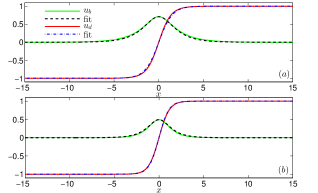
Figure 1: (Color online): Profiles of the fitted single DB solitons, where $u_{d}$ and $u_{b}$ denoted by solid lines respectively correspond to the analytical solution for the single DB case, while dashed and dashed-dotted lines refer to the fitted profiles for the bright and the dark soliton respectively, with (a) $g_{12}=0.85$, and (b) $g_{12}=1.2$. Notice the very good agreement of the fitted solutions upon passing from the miscible to the immiscible regime.

$$E_{\rm dd} = -\frac{11}{3D}\cos^{8}\phi\operatorname{csch}^{7}(2Dx_{0})\sinh(6Dx_{0})+\frac{4}{D}\cos^{4}\phi\operatorname{csch}^{2}(2Dx_{0})\Big{[}-1+2Dx_{0}\coth(2Dx_{0})\Big{]}$$ (19)

$$+ \frac{1}{3D}\cos^{8}\phi\operatorname{csch}^{7}(2Dx_{0})\Big{[}12Dx_{0}\left(9\cosh(2Dx_{0})+\cosh(6Dx_{0})\right)-27\sinh(2Dx_{0})\Big{]}$$

$$+ \frac{1}{3}D\cos^{4}\phi\operatorname{csch}^{5}(2Dx_{0})\Big{[}-24Dx_{0}\cosh(2Dx_{0})+9\sinh(2Dx_{0})+\sinh(6Dx_{0})\Big{]}$$

$$- \frac{4}{3D}\cos^{6}\phi\operatorname{csch}^{5}(2Dx_{0})\Big{[}-24Dx_{0}\cosh(2Dx_{0})+9\sinh(2Dx_{0})+\sinh(6Dx_{0})\Big{]}$$

$$+ \frac{1}{3}D\cos^{2}\phi\Big{[}-24Dx_{0}\operatorname{csch}^{3}(2Dx_{0})\cosh(2Dx_{0})+12\operatorname{csch}^{2}(2Dx_{0})\Big{]},$$

$$E_{\rm bb} = -4\eta^{2}k^{2}x_{0}\operatorname{csch}(2Dx_{0})\cos\Delta\theta+2\eta^{2}D\operatorname{csch}^{3}(2Dx_{0})\cos\Delta\theta\Big{[}-Dx_{0}\left[3+\cosh(4Dx_{0})\right]\Big{]}$$ (20)

$$+ \frac{4}{D}g_{22}\eta^{4}\operatorname{csch}^{3}(2Dx_{0})\cos\Delta\theta\Big{[}-4Dx_{0}+\sinh(4Dx_{0})\Big{]}-8\mu\eta^{2}x_{0}\operatorname{csch}(2Dx_{0})\cos\Delta\theta$$

$$+ \frac{4}{D}g_{22}\eta^{4}\operatorname{csch}^{2}(2Dx_{0})\left(1+2\cos^{2}\Delta\theta\right)\Big{[}-1+2Dx_{0}\coth(2Dx_{0})\Big{]}$$

$$+ 2\eta^{2}D\operatorname{csch}^{3}(2Dx_{0})\cos\Delta\theta\sinh(4Dx_{0}),$$

$$E_{\rm db} = 8g_{12}\eta^{2}x_{0}\operatorname{csch}(2Dx_{0})\cos\Delta\theta-\frac{8}{D}g_{12}\eta^{2}\cos^{2}\phi\operatorname{csch}^{2}(2Dx_{0})\Big{[}-1+2Dx_{0}\coth(2Dx_{0})\Big{]}$$ (21)

$$+ \frac{4}{3D}g_{12}\eta^{2}\cos^{4}\phi\operatorname{csch}^{5}(2Dx_{0})\Big{[}-24Dx_{0}\cosh(2Dx_{0})+9\sinh(2Dx_{0})+\sinh(6Dx_{0})\Big{]}$$

$$+ \frac{4}{D}g_{12}\eta^{2}\cos^{4}\phi\operatorname{csch}^{5}(2Dx_{0})\cos\Delta\theta\Big{[}4Dx_{0}\left[2+\cosh(4Dx_{0})\right]-3\sinh(4Dx_{0})\Big{]}$$

$$- \frac{4}{D}g_{12}\eta^{2}\cos^{2}\phi\operatorname{csch}^{3}(2Dx_{0})\cos\Delta\theta\Big{[}-4Dx_{0}+\sinh(4Dx_{0})\Big{]}.$$

From these equations, the asymptotic results of Eqs. (16)-(18) can be recovered by expanding with respect to $\exp(-2Dx_{0})$. A key realization is that both the bright-bright soliton energy $E_{bb}$ and the cross-component interaction energy $E_{db}$ depend on $\cos(\Delta\theta)$, i.e., on the relative phase and their contribution appears at the same order. Hence, the key underlying intuition of OP bright solitons yielding attraction that will counteract the repulsion of the dark solitons enabling the existence of equilibria may not be sufficient, in terms of providing quantitatively accurate results. The significant contribution of the interaction of the dark solitary waves of one component with the bright ones of the other must be factored in. On the other hand, we also see why, at least in principle, a bound state is possible. The different asymptotic rates of decay of the dark soliton interaction, i.e. faster decaying as $\exp(-4Dx_{0})$ and dominant at shorter distances [see also Eq. (16)], with the bright (and DB) interaction, more slowly decaying as $\exp(-2Dx_{0})$ and dominant at longer distances [see Eqs. (17)-(18)], may create the possibility of an equilibrium, especially for the OP bright soliton scenario.

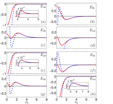
Figure 2: (Color online): Comparison between the exact (solid red lines) and the approximate (dashed blue lines) expressions, within the Hamiltonian variational formulation, for the individual interaction energies [see Eqs. (19)-(21) and Eqs. (16)-(18)] for IP bright soliton components. From top left to bottom right shown are $E_{dd}$, $E_{bb}$, $E_{db}$ and $E_{tot}$ respectively. $(a)$-$(d)$ and $(e)$-$(h)$ correspond to $g_{12}=0.85$ and $g_{12}=1.2$, respectively. In all cases the inset provides a magnified version of the respective extremum.

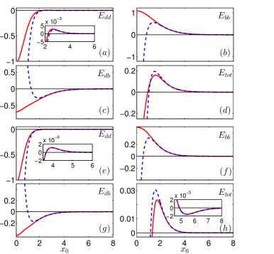
Figure 3: (Color online): Same as Fig. 2 but for OP bright soliton components.

III Numerical Results

Before we embark into an examination of the energies for the different values of the parameters, it is relevant to address the issue of how good the fit of the single DB is with respect to the analytically available expression of Eqs. (7)-(8). Recall, once again, that the expressions of Eqs. (9)-(12) are not used, hence the inverse width parameter $D$ and the bright soliton amplitude parameter $\eta$ are obtained from the exact numerical –up to the prescribed accuracy– single soliton solution upon fitting. As shown in Fig. 1, and in line with the findings of ef , the analytical expression [see Eqs. (7)-(8)] is in very good agreement with the numerically obtained solution for $g_{12}$ in the immiscible regime [see Fig. 1 $(b)$], and especially as $g_{12}$ becomes large. On the other hand, in the miscible regime for $g_{12}$, the tendency of the components to overlap deteriorates the quality of the approximation, especially for $g_{12}\ll 1$ [see Fig. 1 $(a)$]. We remind the reader that the miscibility-immiscibility threshold (after rescaling) is given by $g_{12}^{2}=g_{22}$ aochui . Hence, we expect our analytical approximation to be progressively more accurate as we go deeper into the immiscible regime and to be least adequate for ratios of inter- to intra-component interactions well below unity. Moreover, the improved quality of the fit is also assisted by the fact that upon increasing $g_{12}$ while keeping $\mu$ fixed, a steady decrease of the bright amplitude is observed (cf. also Fig. 6$(i)$ below). This acts in favor of the tanh-sech ansatz as it brings the system closer to the (integrable again) dark-only single- component limit.

We now turn to an examination of the different energy contributions for the IP case in Fig. 2 and for the OP case in Fig. 3. Focusing on stationary solutions, we choose $\phi=0$, $k=0$ and $\Delta\theta=0$ (IP) or $\Delta\theta=\pi$ (OP). The chemical potential ratio is fixed to $\mu=\frac{2}{3}$. At varying $g_{12}$ we numerically identify the single-DB profile and extract the effective values of $D$ and $\eta$ by fitting the tanh-sech ansatz to it. As in most of the cases that will follow, we provide a representative case example in the miscible regime with $g_{12}=0.85$ and another in the immiscible regime with $g_{12}=1.2$. The remaining rescaled nonlinearity coefficient has been fixed to $g_{22}=0.95$, motivated by the relevant ratios in the case of ⁸⁷Rb. Starting with the case of the dark-dark soliton interaction [Fig. 2 $(a)$, $(e)$], we observe that it looks “attractive” in the sense that a regular particle would tend towards the center, upon the imposition of such a potential energy landscape. Yet, the negative effective mass of the DB solution frantz should be factored in and in that case, indeed the interpretation is one of repulsion, as expected from the above. The top right and bottom left panels of each quartet of panels in Fig. 2, represent respectively $E_{bb}$ [Fig. 2 $(b)$, $(f)$], and $E_{db}$ [Fig. 2 $(c)$, $(g)$] confirming their opposite trend as well as their comparable value. In the IP case, at large distances, the bright-bright interaction is repulsive, while the DB is attractive. In the results shown, both the exact, Eqs. (19)-(21), and the asymptotic, Eqs. (16)-(18), forms of the energy expressions are given (denoted by solid red and dashed blue lines respectively in Figs. 2, 3). Expectedly, they coincide at large $x_{0}$ where $\exp(-2Dx_{0})$ becomes small, while at short distances the deviations can be substantial, even qualitatively. It should be borne in mind here that neither of these expressions is sufficiently good when the DB solitons are sufficiently close (distances $0<x_{0}<1.5$ typically for our results herein). There, the solitons are essentially overlapping and hence, the superposition ansatz of Eqs. (13)-(14) clearly fails.

Coming to the main conclusion of the theoretical analysis, let us examine the OP case of Fig. 3. The key panel to consider is that of the total energy [Fig. 3 $(d)$, $(h)$]. The identification of a local maximum there for both the cases of $g_{12}=0.85$ and $g_{12}=1.2$ (and for all values of $g_{12}$ in between) suggests the existence of an effective local minimum representing a stable equilibrium, at least in as far as the OP vibration of the two DBs around it is concerned. Note here that due to the translational invariance, the two-DB center of mass can always be displaced freely. This prediction can be tested against the direct numerical computations of the original PDE system of Eqs. (4)–(5). In the latter, we use a fixed point (Newton-Raphson) iteration to obtain the OP equilibrium kelley . Subsequently, we identify the location of the (coincident between the two components) soliton center and compare it to the corresponding theoretical value. The result is shown in Fig. 4 and is quite satisfactory in terms of capturing the relevant trend. The increasing tendency of the equilibrium $x_{0}$ as a function of $g_{12}$ as the miscibility threshold is crossed and as we move deeper into the immiscibility regime can be intuitively understood as follows. In the OP case, the bright-bright interaction [Fig. 2 $(b)$, $(f)$] is attractive at the tails and the DB interaction is repulsive [Fig. 2 $(c)$, $(g)$]. This becomes even more pronounced as $g_{12}$ increases as can be seen from Eq. (21) [see also Eq. (18)] and thus the equilibrium is expected to be found at larger distances due to this stronger repulsion.

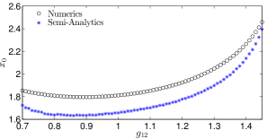
Figure 4: (Color online): Equilibrium location $x_{0}$ as a function of the nonlinear coefficient $g_{12}$ for OP bright soliton components. Black circles depict the numerically obtained two DB soliton center, while blue stars correspond to the semi-analytical prediction of the effective particle picture.

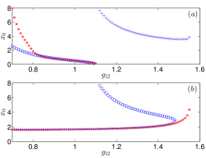
Figure 5: (Color online): Variationally predicted equilibrium positions between two DB solitons as a function of $g_{12}$. $(a)$ [$(b)$] shows the extrema for IP (OP) bright soliton components. Blue circles denote the location of the minimum of the total energy $E_{tot}$, while blue crosses correspond to the respective maxima. Red stars refer to the extrema predicted via the fully numerical evaluation of the energy (see text). The chemical potential is fixed to $\mu=2/3$.

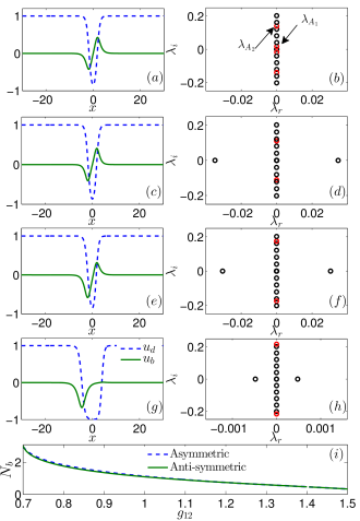
Figure 6: (Color online): Left column: $(a)$ anti-symmetric stationary DB soliton pair for $g_{12}=1.1$, $(c)$ anti-symmetric state with $g_{12}=1.3$, $(e)$ asymmetric state for $g_{12}=1.1$, and $(g)$ fully asymmetric D-DB state for $g_{12}=0.95$. Right columns [$(b)$ to $(h)$] are the associated BdG spectra, where the lowest twenty eigenvalues are shown with (black/red) circles. In all cases red circles denote the anomalous modes. $\lambda_{A_{1}}$, and $\lambda_{A_{2}}$, (indicated by black arrows) are the two modes related to the observed symmetry breaking, and the OP vibration of the 2-DB state respectively. $(i)$: $N_{b}$ as a function of $g_{12}$ for the two different branches sg .

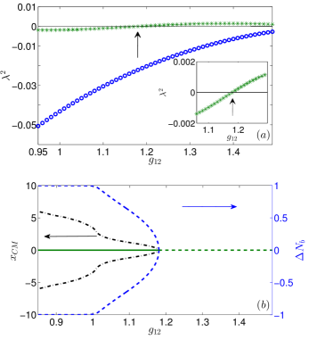
Figure 7: (Color online): $(a)$ Trajectories of the squared eigenvalues of the two anomalous modes, $\lambda^{2}$ upon varying $g_{12}$ for the anti-symmetric stationary solutions of Eqs. (4)-(5). Blue circles correspond to the trajectory of the mode related to the OP vibration of the 2-DB state. Green stars denote the trajectory of the mode responsible for the symmetry breaking bifurcation that occurs at $g_{12_{cr}}=1.18$. $(b)$ bifurcation diagram, obtained via measuring the center of mass and the mass imbalance of the bright component (see the text for the relevant definitions) as functions of $g_{12}$. The two arrows indicate the different axes used. Four branches are identified: three unstable ones (dashed-dotted black and dashed blue/green lines) and a stable branch (solid green line). Notice that the asymmetric branches exist before the critical point and are unstable, i.e. the pitchfork is subcritical.

Now, we turn to a series of spurious features that the theory may produce. By far the most significant is that if, by comparison, we examine the total energy in the bottom right panels of the quartets in Fig. 2 $(d)$, $(h)$, we will notice the existence of a local minimum, which is tantamount to an effective energy maximum, and is expected to correspond to a saddle point in the case of the IP bright solitons (within the two DBs). This is found to exist only for sufficiently small $g_{12}$’s i.e., it exists for $g_{12}=0.85$, but not for $g_{12}=1.2$ (cf. $(a)$-$(d)$ vs. $(e)$-$(h)$ quartets of panels in Fig. 2). This feature, if present, would suggest that while in the IP case the dark-dark and bright-bright interactions are both repulsive, the DB one is attractive and enough to counter both to produce an equilibrium, albeit an unstable one. However, an extensive effort to identify this feature in the PDE did not lead to fruition. While we cannot fully exclude the possibility that such an equilibrium exists, both our fixed point iteration results and the direct numerical simulations (presented below) suggest its absence. Our explanation for this “negative” result is that this equilibrium arises at relatively short distances and rapidly moves towards the origin. The relevant dependence on $g_{12}$ can be found in Fig. 5 $(a)$ denoted by blue circles. Here, we observe that the equilibrium occurs at moderate distances only for the smallest values of $g_{12}$ considered (close to $0.7$) where we know that the ansatz is the worst (within our range) as regards capturing the true waveform of the DB soliton. As $g_{12}$ increases, while the ansatz gradually improves, the equilibrium distance rapidly decreases, rendering the ansatz inadequate due to the overlap (and constructive interference in this case) between the solitons. Therefore, the individual character of the solitons is lost and hence the ansatz again fails. Thus, we intend this part as a cautionary tale about the potential inadequacies of the variational ansatz, either due to the failure of the profile of Eqs. (7)-(8) or because of the failure of the two-soliton waveform.

An additional feature that we have identified when taking the Hamiltonian variational formulation at face value can be seen in the insets of Figs. 2 and 3, when looking at sufficiently large distances in the case of $g_{12}=1.2$. Examining the total energy plots at the bottom right panel of each of the aforementioned figures [Fig. 2 $(h)$ and Fig. 3 $(h)$], we find that an additional extremum appears to arise. The trajectory of this extremum (in both cases) is illustrated in Fig. 5 $(a)$ (blue crosses) for the IP and in Fig. 5 $(b)$ (blue circles) for the OP case. A careful inspection of the relevant energy scales of Figs. 2 and 3 confirms that this is a miniscule effect of the order of $10^{-5}$, in this case example. Again, an extensive search for corresponding stationary solutions on the PDE level remained unsuccessful, which suggests that the miniscule large-$x_{0}$ extrema of the $E_{tot}$ energy curves may be artifacts of the variational approach that are absent in the true dynamics.

In fact, in an attempt to explore these spurious extrema further and to disentangle the errors stemming from the single-DB fitting process and its concomitant identification of $D$ and $\eta$ on the one hand and the two-DB ansatz in Eqs. (13)-(14) on the other hand, we also attempted a “purely numerical” construction of the energy. That is, upon identifying the single-DB waveform, we numerically constructed the 2-DB profile, multiplying two darks and adding (for the IP case) two brights centered at varying distances, i.e. in the spirit of Eqs. (13)-(14) but avoiding the tanh-sech fit. Then, we numerically evaluated the resulting energy by numerically integrating the expression of Eq. (6). This side-steps the inadequacies of the single soliton ansatz, yet it does not avoid the issues of the two soliton ansatz upon close proximity of the bright solitons. Within this latter approach, we do not find the miniscule large-$x_{0}$ maximum in $E_{tot}$ for the IP case, suggesting that this is a spurious feature induced by the imperfect tanh-sech fit. In contrast, the more substantial in-phase energy minimum for $g_{12}\lesssim 1.1$ qualitatively persists even without performing this fit [see red stars in Fig. 5 $(a)$]. Its predicted quantitative position, however, is shifted to considerably larger values of $x_{0}$ for small $g_{12}$. This discrepancy highlights the inaccuracies of the fit in the miscible regime, but the existence of the spurious IP minimum itself seems to be induced not by the imperfect single-DB fit but by the construction of the two-DB ansatz. Finally, in the OP case the fully numerical variational approach predicts a bond length of the DB pair that agrees well with that from the tanh-sech fit approach, underlining the robustness of this key result. The fit-based method also predicts a local minimum in $E_{tot}$ which annihilates the bound-state maximum in a saddle-center bifurcation at $g_{12}=1.48$. Without the tanh-sech fit, the bound state is predicted to persist up to $g_{12}=1.55$, beyond which the bright norm is zero [see red stars in Fig. 5 $(b)$]. In the numerical variational framework we do not see a minimum in $E_{tot}$ here, but possibly the aforementioned termination of the bound-pair branch could also be caused by a saddle-center bifurcation happening at large $x_{0}$ (where all energies become extremely small and ultimately lie below our numerical resolution).

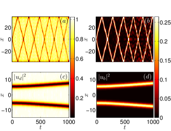
Figure 8: (Color online): Typical examples of the space-time evolution of the density of a 2-DB soliton state for IP bright solitons. $(a)$, $(b)$ densities for $g_{12}=0.85$ and equilibrium distance $x_{0}=1.37$. $(c)$, $(d)$ same as the above, but for $g_{12}=1.2$ and $x_{0}=5.45$. In both cases $(a)$, $(c)$ [$(b)$, $(d)$] refer to the evolution of the dark [bright] soliton component.

It is then clear that out of the four possible extrema presented in the in and out of phase cases, only the out of phase equilibrium is relevant for the system. Hence, we explore the latter further, before delving into the associated dynamics. To assess the stability of this fixed point, we perform a BdG analysis, linearizing around the equilibrium as follows:

$$u_{d} = u_{d}^{(eq)}+\left(a(x)e^{-i\omega t}+b^{\star}(x)e^{i\omega^{\star}t}\right),$$ (22)

$$u_{b} = u_{b}^{(eq)}+\left(c(x)e^{-i\omega t}+d^{\star}(x)e^{i\omega^{\star}t}\right).$$ (23)

The resulting linearization system for the eigenfrequencies $\omega$ (or equivalently eigenvalues $\lambda=i\omega$) and eigenfunctions $(a,b,c,d)^{T}$ is solved numerically. If modes with purely real eigenvalues (genuinely imaginary eigenfrequencies) or complex eigenvalues (eigenfrequencies) are identified, these are tantamount to the existence of an instability revip . Remarkably, indeed this is the case, as we increase $g_{12}$. An eigenvalue pair crosses the origin and becomes real, resulting in an exponential instability that we will trace soon in the dynamics as well. Presently, we inquire which mode could be responsible for such an instability. We note that in addition to 6 modes in the spectrum at $\lambda=\omega=0$ due to symmetries (the conservations of $N_{d}$ and $N_{b}$, as well as due to the momentum-conservation-inducing invariance with respect to translation), there are two additional modes of interest that are “hidden” within the continuous spectrum of the problem, see the BdG spectrum in the middle right panel of Fig. 6 where black arrows indicate the modes in question denoted by red circles. These modes are so-called anomalous or negative energy modes. They possess negative energy or negative Krein signature skryabin . The mode energy (or Krein signature) is defined as

$$K=\omega\int\Big{(}|a|^{2}-|b|^{2}+|c|^{2}-|d|^{2}\Big{)}dx,$$ (24)

in a multi-component system like the one considered herein. Our computations show that there are two such modes in the system. One is the anticipated one, related to the out-of-phase vibration of the two DB solitons ($\lambda_{A_{2}}$ in Fig. 6 $(b)$). However, as suggested by the energetics discussed previously it remains stable (pertaining to oscillations in the effective energy landscape discussed above). The second mode ($\lambda_{A_{1}}$ in Fig. 6 $(b)$) is the one associated with symmetry breaking of the bright component. I.e., adding the corresponding eigenvector to the bright component breaks its symmetry and results in two bright solitons of unequal amplitudes. It is the latter mode that destabilizes at the instability threshold of the out of phase configuration. The existence (and destabilization) of such a mode suggests the presence of a pitchfork bifurcation associated with the symmetry breaking. Indeed, we have been able to identify the asymmetric branches related to this pitchfork bifurcation. Interestingly, the branches exist before the critical point of the anti-symmetric solution destabilization and are unstable themselves. That is to say the pitchfork is subcritical. A similar, yet crucially different, bifurcation mechanism was identified in the work of et in the presence of a parabolic trap. In that setting, an effective single-component description was found to be applicable, where the two dark solitons together with the trap act as an approximately static double-well potential for the bright component. Within a two-node tight-binding approximation this then maps to the bosonic Josephson junction model which features a symmetry-breaking supercritical pitchfork bifurcation from the OP branch. Correspondingly, the emerging asymmetric modes are found to be stable in the trapped framework, while they are unstable in our present setting [see the linearization spectra in Figs. 6$(f,h)$], highlighting the fundamentally different nature of the symmetry-breaking pitchfork bifurcations in the trapped and untrapped cases, respectively.

In Fig. 6 $(a)$, an anti-symmetric solution is shown together with its linearization spectrum for $g_{12}=1.1$ [Fig. 6 $(b)$]. Two anomalous modes are identified, indicated by the arrows. The lowest of these eigenvalues, namely $\lambda_{A_{1}}$, moves towards zero with increasing $g_{12}$ and eventually crosses to the real axis, which signals the pitchfork bifurcation. In panels $(c)$-$(d)$, an example of an anti-symmetric equilibrium state is illustrated past its destabilization threshold. Furthermore, in panels $(e)$-$(h)$ asymmetric solutions are identified and shown together with their respective linearization eigenvalues manifesting their instability. In particular, $(e)$-$(f)$ correspond to an asymmetric solution for $g_{12}=1.1$, providing a straightforward comparison of its BdG spectrum with the respective spectrum of the anti-symmetric state in $(a)$-$(b)$. Notice in particular the absence of the anomalous mode $\lambda_{A_{1}}$. Moreover, in panels $(g)$-$(h)$ another example of the asymmetric state at smaller $g_{12}$ is depicted. Here, a total transfer of mass of the bright component to one of the dark solitons has occurred, resulting in a bound state of one purely dark and one dark-bright soliton. Note again the crucial difference to the self-trapped states of the bosonic Josephson junction here, since in the present setting the pitchfork bifurcation phenomenology arises in a spatially homogeneous setting. Finally, Fig. 6$(i)$ illustrates the decrease of the bright soliton norm upon increasing $g_{12}$ for both the anti-symmetric and asymmetric solitonic states.

All of the above findings are summarized in Fig. 7. In particular, Fig. 7 $(a)$ shows the trajectory of the squared eigenvalues of the two anomalous modes as $g_{12}$ increases. Notice that among these two trajectories the lowest one (blue circles) asymptotically tends to zero, and as such it remains stable for all values of $g_{12}$. This trajectory corresponds to the OP vibration of the two DB state. However, a completely different picture is painted by the trajectory of the second mode (green stars). Closely following this trajectory [see also the inset in Fig. 7 $(a)$] we see that this mode destabilizes at $g_{12_{cr}}=1.18$ (which corresponds to the eigenvalue zero crossing). This destabilization signals the bifurcation and the emergence of the upper (black dotted) branch. Note that for clarity reasons we only show values of $g_{12}$ in the vicinity of the bifurcation. The respective bifurcation diagram is shown in Fig. 7 $(b)$. To obtain this diagram we simply measure the center of mass between the two bright solitons in the second component, i.e. $x_{CM}=\int_{-\infty}^{\infty}x|u_{b}|^{2}dx/\int^{\infty}_{-\infty}|u_{b}|^{2}dx$, upon varying $g_{12}$. This way, we can identify both the stable anti-symmetric branch [solid green line in Fig. 7 $(b)$] as well as the three unstable branches, two asymmetric and one anti-symmetric [see dashed-dotted black lines and dashed-dotted green line respectively in Fig. 7 $(b)$]. Notice that the asymmetric branches exist before the critical point, verifying the subcritical pitchfork nature of the relevant bifurcation. It is also worth mentioning the “neck” in $x_{CM}$ that occurs at the immiscibility to miscibility transition. This feature is found to coincide with a change in the character of the symmetry-broken soliton configuration, i.e. the transition from a gradually asymmetric DB-DB pair as in Fig. 6 $(e)$ to a maximally asymmetric dark/dark-bright (D-DB) state as in Fig. 6$(g)$. This is seen in the relative bright imbalance defined as $\Delta N_{b}\equiv\left(\int_{-\infty}^{0}|u_{b}|^{2}dx-\int^{\infty}_{0}|u_{b}|^{2}dx\right)/\int^{\infty}_{-\infty}|u_{b}|^{2}dx$ and shown in dashed blue lines in Fig. 7$(b)$.

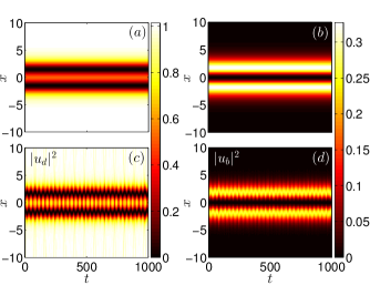
Figure 9: (Color online): Typical examples of the space-time evolution of the density of a stationary 2-DB soliton state for OP bright solitons and $g_{12}=0.85$. Evolution of the dark soliton density $(a)$, and the respective bright one $(b)$, initialized at the predicted equilibrium distance with $x_{0}=1.65$. $(c)$, $(d)$ same as the above, but slightly inside of the predicted fixed point at $x_{1}=1.45$.

Finally, we turn to direct numerical simulations corroborating the existence and stability results presented above. Firstly, in Fig. 8, we examine the (theoretically predicted, yet argued as spurious) equilibria of the theoretical energy analysis presented above. We see in the figure that both in the case of $g_{12}=0.85$ [Fig. 8 $(a)$, $(b)$] and in that of $g_{12}=1.2$ [Fig. 8 $(c)$, $(d)$], as well as in all the additional cases that we have examined (not shown here), repulsive dynamics is manifested between the two DBs. We have tried different distances, smaller as well as larger than the equilibrium one, always finding this type of repulsive behaviour. If the prediction of a saddle point was an accurate one, the solitons should have moved inward (rather than outward, i.e., featuring attraction) when initially positioned below the equilibrium distance. In fact, what we find is that at short distances the soliton repulsion is fairly dramatic. As the figure suggests, this is partially the result of constructive interference in the case of our initial conditions. I.e., while adjusting from an initial profile through a transient stage, the solitary waves emit radiative wavepackets. Some of these move outward (and do not pose concerns, provided that the integration domain is sufficiently large). However, some of these move inward, constructively interfere and exert upon return a substantial effective force which assists the solitons towards initiating their outward trajectory. Thus, our direct simulations also confirm the expectation that the variationally predicted fixed point is an artifact of the ansatz and is dynamically absent in the IP case.

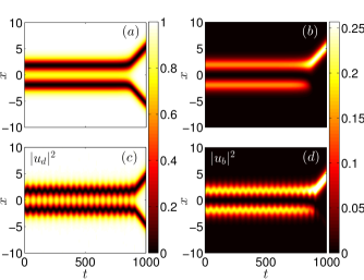
Figure 10: (Color online): Same as Fig. 9 but for $g_{12}=1.2$, i.e. well inside the immiscible regime. $(a)$, $(b)$ initialization at $x_{0}=1.78$, coinciding with the semi-analytical prediction of the stationary 2-DB state. $(c)$, $(d)$ initialization at $x_{1}=1.58$. Notice that symmetry breaking occurs towards the end of the simulation, resulting in an almost complete transfer of mass from the left bright soliton to the right one [$(b)$, $(d)$ counterpart of each doublet].

Hence, we hereafter focus on the OP case. We explore the latter both when initiated at equilibrium, as well as when initiated near equilibrium. This is done for the case of $g_{12}=0.85$ in Fig. 9, as well as for that of $g_{12}=1.2$ in Fig. 10. In the former case, our BdG stability analysis predicts that the anti-symmetric bright soliton configuration (and the whole DB pair) will be dynamically robust. Indeed, this is what we observe; when initializing at the equilibrium, [Fig. 9 $(a)$, $(b)$] the solitary waves stay put, while when initiating at slightly smaller or larger distances [Fig. 9 $(c)$, $(d)$], we simply excite the stable OP vibrational mode of the two-soliton molecule. However, a fundamentally different picture is shown in Fig. 10 for the case of $g_{12}=1.2$. Here, while for a long time the configuration appears to be quiescent eventually for times $t>800$, the bright soliton redistributes its mass dramatically [see Fig. 10 $(b)$], resulting in a strong repulsion between the ensuing single DB (with a much larger bright soliton mass) and the dark soliton (respectively, stripped of its soliton mass, Fig. 10 $(a)$). This leads to the strong separation of the solitary waves as a result of the dynamics. The same feature can be seen in the case of oscillations around the equilibrium, Fig. 10 $(c)$, $(d)$; while the solitons appear robust for many oscillation cycles, we can see them eventually redistributing the bright component [Fig. 10 $(d)$] and splitting as a result. Although the instability appears to be dramatic and instantaneous, a more careful monitoring of the system suggests otherwise. In particular in Fig. 11, we monitor the evolution of the bright density at the central point between the two solitons. Examining the relevant diagnostic in a semilog scale, we clearly infer that the instability is building over the entire horizon of the simulation, featuring a remarkable exponential growth over many orders of magnitude until eventually it produces an effect of order unity resulting in the symmetry breaking. We confirm by examining the growth rate of this exponential growth, that it is indeed occurring with the unstable eigenvalue of the two-DB state.

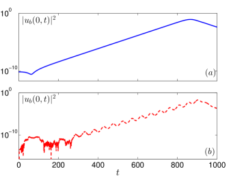
Figure 11: (Color online): Semi-logarithmic representation, showing the central bright density between the two solitons throughout the propagation depicted in Fig. 10. This way, we monitor the exponential growth of the instability, that clearly builds up from the first instant (initially hidden in the noise below our numerical accuracy threshold) and fully manifests itself when it becomes of order $\mathcal{O}(1)$ Panels $(a)$ and $(b)$ correspond to the symmetry breaking observed in panels $(b)$ and $(d)$ of Fig. 10.

IV Conclusions and Future Challenges

In the present work, the intriguing problem of DB soliton interactions has been revisited. Motivated by recent experimental studies of the problem, the relevant formulation has been extended in a number of ways. We have considered the effect of general (and beyond integrable) inter-atomic interaction coefficients and identified full analytical expressions of the variational energy-based formulation, rather than solely approximate ones, focusing on the former as being more accurate than the latter. Our aim was to explore the conclusions of the energy based calculation monoparametrically varying the inter-component scattering length. This led to the identification of key additional features in the energy such as the significant role of DB soliton interaction, often overlooked in earlier studies. We carefully considered which of the features of the variational formulation are credible for leading to accurate results and which ones should be discarded and for what reason i.e., which assumptions and approximations in the variational formulation may turn out to fail. Focusing on the predominant nontrivial feature, namely the existence of an equilibrium in the out-of-phase case, we showcased the predictive strength of the formulation and identified a subcritical pitchfork bifurcation instability-inducing scenario that had not been previously observed, to the best of our knowledge. The consequences of the instability were dynamically explored and observed to lead to the key phenomenon of mass redistribution.

There is a multitude of intriguing questions that are worth examining in future efforts. On the one hand, it would be particularly interesting to explore if the variational formulation might predict the potential for symmetry-breaking instability provided the relevant freedom. More concretely, we can utilize an ansatz for the bright solitons involving two hyperbolic secants with distinct amplitudes $\eta_{1}$ and $\eta_{2}$. An important question is: is this sufficient (as one might hope/expect based on the above description) to observe the instability at the level of the few degree of freedom system? In the context of this symmetry-breaking, it would moreover be interesting to explore the crossover from our present untrapped setting with its subcritical pitchfork bifurcation to the harmonically trapped case where in et a supercritical pitchfork bifurcation has been found to destabilize the out-of-phase mode. Extensions of the present considerations would also be worthwhile to pursue in other settings including ones involving a higher number of components, as well as higher dimensions. In the former one, solitary waves such as dark-dark-bright and dark-bright-bright ones DDB have been predicted, so it would be interesting to see how the relevant phenomenology generalizes. In the latter one, the role of dark solitons is played by vortices kody ; pola . Such “vortex-bright” solitons are quite robust and furthermore their vorticity is topologically protected, so it would be interesting to examine whether they would form similar bound states and what the stability and dynamics of the latter would be. Studies along these directions are reserved to future works.

References

- (1) P.G. Kevrekidis, D.J. Frantzeskakis, Reviews in Physics 1, 140 (2016).
- (2) Yu. S. Kivshar and G. P. Agrawal, Optical solitons: from fibers to photonic crystals (Academic Press, San Diego, 2003).
- (3) D. N. Christodoulides, Phys. Lett. A 132, 451 (1988).
- (4) V. V. Afanasjev, Yu. S. Kivshar, V. V. Konotop, and V. N. Serkin, Opt. Lett. 14, 805 (1989).
- (5) Yu. S. Kivshar and S. K. Turitsyn, Opt. Lett. 18, 337 (1993).
- (6) R. Radhakrishnan and M. Lakshmanan, J. Phys. A: Math. Gen. 28, 2683 (1995).
- (7) A. V. Buryak, Yu. S. Kivshar, and D. F. Parker, Phys. Lett. A 215, 57 (1996).
- (8) A. P. Sheppard and Yu. S. Kivshar, Phys. Rev. E 55, 4773 (1997).
- (9) Park Q. Han, and Shin H. J., Phys. Rev. E 61, 3093 (2000).
- (10) Z. Chen, M. Segev, T. H. Coskun, D. N. Christodoulides, and Yu. S. Kivshar, J. Opt. Soc. Am. B 14, 3066 (1997).
- (11) E. A. Ostrovskaya, Yu. S. Kivshar, Z. Chen, and M. Segev, Opt. Lett. 24, 327 (1999).
- (12) Th. Busch, and J. R. Anglin, Phys. Rev. Lett. 87, 010401 (2001).
- (13) C. Becker, S. Stellmer, P. Soltan-Panahi, S. Dörscher, M. Baumert, E.-M. Richter, J. Kronjäger, K. Bongs, and K. Sengstock, Nat. Phys. 4, 496 (2008).
- (14) C. Hamner, J. J. Chang, P. Engels, and M.A. Hoefer, Phys. Rev. Lett. 106, 065302 (2011).
- (15) S. Middelkamp, J. J. Chang, C. Hamner, R. Carretero-González, P. G. Kevrekidis, V. Achilleos, D. J. Frantzeskakis, P. Schmelcher, and P. Engels, Phys. Lett. A 375, 642 (2011).
- (16) D. Yan, J. J. Chang, C. Hamner, P. G. Kevrekidis, P. Engels, V. Achilleos, D. J. Frantzeskakis, R. Carretero-González, and P. Schmelcher, Phys. Rev. A 84, 053630 (2011).
- (17) A. Álvarez, J. Cuevas, F. R.. Romero, C. Hamner, J. J. Chang, P. Engels, P. G. Kevrekidis, and D. J. Frantzeskakis, J. Phys. B 46, 065302 (2013).
- (18) M.A. Hoefer, J. J. Chang, C. Hamner, and P. Engels, Phys. Rev. A 84, 041605(R) (2011).
- (19) D. Yan, J. J. Chang, C. Hamner, M. Hoefer, P. G. Kevrekidis, P. Engels, V. Achilleos, D. J. Frantzeskakis, and J. Cuevas, J. Phys. B: At. Mol. Opt. Phys. 45, 115301 (2012).
- (20) Y. S. Kivshar and W. Kro´likowski, Opt. Commun. 114, 353 (1995).
- (21) A. Weller, J. P. Ronzheimer, C. Gross, J. Esteve, M. K. Oberthaler, D. J. Frantzeskakis, G. Theocharis, and P. G. Kevrekidis, Phys. Rev. Lett. 101, 130401 (2008); G. Theocharis, A. Weller, J. P. Ronzheimer, C. Gross, M. K. Oberthaler, P. G. Kevrekidis, and D. J. Frantzeskakis, Phys. Rev. A 81, 063604 (2010).
- (22) J.H.V. Nguyen, P. Dyke, D. Luo, B.A. Malomed, R.G. Hulet, Nat. Phys. 10, 918 (2014).
- (23) S. Inouye, M. R. Andrews, J. Stenger, H.-J. Miesner D. M. Stamper-Kurn, and W. Ketterle, Nature (London) 392, 151 (1998); J. L. Roberts, N. R. Claussen, J. P. Burke, Jr., C. H. Greene, E. A. Cornell, and C. E. Wieman, Phys. Rev. Lett. 81, 5109 (1998); E. A. Donley, N. R. Claussen, S. L. Cornish, J. L. Roberts, E. A. Cornell, and C. E. Wieman, Nature (London) 412, 295 (2001).
- (24) G. Thalhammer, G. Barontini, L. De Sarlo, J. Catani, F. Minardi, and M. Inguscio, Phys. Rev. Lett. 100, 210402 (2008); S. B. Papp, J. M. Pino, and C. E. Wieman, Phys. Rev. Lett. 101, 040402 (2008).
- (25) C. Chin, R. Grimm, P. Julienne, and E. Tiesinga, Rev. Mod. Phys. 82, 1225 (2010).
- (26) K. M. Mertes, J. W. Merrill, R. Carretero-González, D. J. Frantzeskakis, P. G. Kevrekidis, and D. S. Hall, Phys. Rev. Lett. 99, 190402 (2007).
- (27) Although we use these values of and as “typical”, it is worthwhile to mention that the precise value of the coefficients is still under active investigation, with the most accurate values known presently being those of M. Egorov, B. Opanchuk, P. Drummond, B. V. Hall, P. Hannaford, and A. I. Sidorov, Phys. Rev. A 87, 053614 (2013).
- (28) P. Ao and S. T. Chui Phys. Rev. A 58, 4836 (1998)
- (29) L. P. Pitaevskii and S. Stringari, Bose-Einstein Condensation. Oxford University Press (Oxford, 2003).
- (30) P. G. Kevrekidis, D. J. Frantzeskakis, and R. Carretero-González, The Defocusing Nonlinear Schrödinger Equation, SIAM (Philadelphia, 2015).
- (31) S. V. Manakov, Zh. Eksp. Teor. Fiz. 65, 505 (1973) [Sov. Phys. JETP 38, 248 (1974)].
- (32) C. T. Kelley, Solving Nonlinear Equations with Newton’s Method (Society for Industrial and Applied Mathematics, Philadelphia, 1995).
- (33) D. Yan, F. Tsitoura, P. G. Kevrekidis, and D. J. Frantzeskakis, Phys. Rev. A 91, 023619 (2015).
- (34) D. J. Frantzeskakis, J. Phys. A 43, 213001 (2010).
- (35) Dmitry V. Skryabin, Phys. Rev. A 63, 013602 (2000).
- (36) Note that, for the numerical implementation we use hard-wall-like boundary conditions, specifically a super-Gaussian potential of the form , which introduces an unavoidable discretization of the continuous spectrum. For some parameters we numerically observe collisions of linearization modes from this discretized continuous spectrum with the anomalous modes resulting in oscillatory instability windows; these are likely to depend on the specific boundary conditions and are not explored in more detail here.
- (37) E. T. Karamatskos, J. Stockhofe, P. G. Kevrekidis, and P. Schmelcher, Phys. Rev. A 91, 043637 (2015).
- (38) H. E. Nistazakis, D. J. Frantzeskakis, P. G. Kevrekidis, B. A. Malomed, and R. Carretero-González, Phys. Rev. A 77, 033612 (2008).
- (39) K. J. H. Law, P. G. Kevrekidis, and Laurette S. Tuckerman, Phys. Rev. Lett. 105, 160405 (2010).
- (40) M. Pola, J. Stockhofe, P. Schmelcher, and P. G. Kevrekidis, Phys. Rev. A 86, 053601 (2012).