The $K$-band luminosity functions of cluster galaxies

Abstract

We derive the galaxy luminosity function in the $K_{s}$ band for galaxies in 24 clusters to provide a local reference for higher redshift studies and to analyse how and if the luminosity function varies according to environment and cluster properties. We use new, deep $K$ band imaging and match the photometry to available redshift information and to optical photometry from the SDSS or the UKST/POSS: $>80\%$ of the galaxies to $K\sim 14.5$ have measured redshifts. We derive composite luminosity functions, for the entire sample and for cluster subsamples . We consider the luminosity functions for red sequence and blue cloud galaxies. The full composite luminosity function has $K^{*}=12.79\pm 0.14$ ($M_{K}=-24.81$) and $\alpha=-1.41\pm 0.10$. We find that $K^{*}$ is largely unaffected by the environment but that the slope $\alpha$ increases towards lower mass clusters and clusters with Bautz-Morgan type $<$ II. The red sequence luminosity function seems to be approximately universal (within errors) in all environments: it has parameters $K^{*}=13.16\pm 0.15$ ($M_{K}=-24.44$) and $\alpha=-1.00\pm 0.12$ (for all galaxies). Blue galaxies do not show a good fit to a Schechter function, but the best values for its parameters are $K^{*}=13.51\pm 0.41$ ($M_{K}=-24.09$) and $\alpha=-1.60\pm 0.29$: we do not have enough statistics to consider environmental variations for these galaxies. We find some evidence that $K^{*}$ in clusters is brighter than in the field and $\alpha$ is steeper, but note this comparison is based (for the field) on 2MASS photometry, while our data are considerably deeper.

1 Introduction

The galaxy luminosity function (hereafter LF) provides a fundamental description of the gross properties of galaxy populations. The first task of theories of galaxy formation and evolution is to match the observed LF, a task that has been somewhat difficult as uncertain baryonic effects (e.g., star formation) and feedback are needed to transform the mass function of dark matter halos into observables (e.g., see Contreras et al. 2016; Narayanan 2016 and references therein).

Clusters of galaxies, as the largest virialised systems in the Universe, have played an important role in this field. The LF of cluster galaxies can be determined, even at high redshifts, via simple photometry, as the overdensity with respect to the surrounding fields allows us to correct for contamination (from non members in the foreground and background) by statistical means, without expensive redshift surveys. However, the faint end of the LF is still in dispute, even at low redshifts, as the steeply rising field counts lead to progressively more unfavourable statistics. Studies of nearby clusters have claimed that the LF consists of a Schecher function at the bright end and a steeply rising power law at the faint end (e.g., Moretti et al. 2015; Lan et al. 2016) but others have found a single Schechter function (e.g., Rines & Geller 2008; Sanchez-Janssen et al. 2016).

Ideally, the LF should be measured in a band where luminosity matches stellar mass as closely as possible, in order to better compare with the predictions of theoretical models and avoid the effects of star formation on bluer (optical) bands. The infrared $K$ band has been shown to provide a reasonable approximation to the underlying stellar mass function, and even dynamical mass (Gavazzi et al., 1996; Bell & de Jong, 2001). In addition, both evolutionary and $k$-corrections are known to be small and to vary slowly with redshift or with galaxy type. For these reasons, the $K$-band LF has been used as a probe of the evolution of galaxy populations (e.g., see Capozzi et al. 2012 and references therein).

There are relatively few local cluster LFs in the $K$-band, owing to the comparatively small size of infrared detectors until recently. In our previous work, we studied the Coma cluster using a complete spectroscopic sample for its inner $25^{\prime}$ (De Propris et al., 1998). Skelton et al. (2009) determined a LF for the Norma cluster and Merluzzi et al. (2010) derived a composite LF for galaxies in the Shapley supercluster. Previously, De Propris & Christlein (2009) presented a composite LF for 10 clusters from the 2dF sample of De Propris et al. (2003). Here we determine the LF for 24 of these clusters, with new infrared imaging and high redshift completeness. The following sections describe the data and analysis, present the results and discuss these in the context of previous work and models for galaxy formation and evolution. Here, we assume the standard cosmological parameters $\Omega_{M}=0.27$, $\Omega_{\Lambda}=0.73$ and $H_{0}=73$ km s^-1 Mpc^-1.

2 Data and Analysis

We have carried out deep $K$-band imaging for a set of 24 clusters from the sample of De Propris et al. (2003) in order to derive composite $K$ band LFs. Our data consist of 300s images in the $K_{s}$ filter obtained at the CTIO 4m telescope, with either the Infrared SidePort Imager (ISPI – Probst et al. 2003) or the NOAO Extremely Wide Field Infrared Mosaic (NEWFIRM – Autry et al. 2003) for 20 clusters, covering the clusters out to their Abell radius (1.5 $h^{-1}$ Mpc). For a few clusters (4/24) we have instead used available UKIDSS data from the Large Area Survey (Data Release 10) as we could not observe them from CTIO in the available time. Table 1 summarizes the data used and basic properties of the clusters.

We have elected not to use 2MASS (Skrutskie et al., 2006) photometry, except for purposes of calibration, as this is known to miss a considerable fraction of the flux for bright galaxies and to be incomplete for fainter ones (Andreon, 2002; Kirby et al., 2008). We confirm this by comparison with our photometry: on average, 2MASS magnitudes (we use the homogeneous $14^{\prime\prime}$ aperture for reference, which should be large enough to include all the flux) are systematically $\sim 0.3$ mag. fainter than ours. Further, some galaxies are already missing from 2MASS (or misclassified as stars) at $K>13$. However, our much deeper data (300s on a 4m class telescope, compared to the 52s exposures on a 1.3m telescope for 2MASS) should not suffer from these issues.

For ISPI and NEWFIRM imaging we observed using a five point dithering pattern. For NEWFIRM, the dithering steps were large enough to remove the $\sim 30^{\prime\prime}$ gaps between the four detectors. Where the Abell radius was larger than the size of the detector, we mosaicked to cover the entire field (this took several ISPI fields, as the field of view is only $\sim 10^{\prime}$, but only small NEWFIRM mosaics). ISPI data were reduced following the conventional pattern for infrared data: removal of flatfield with on and off dome light flats, median sky removal from neighbouring (in time) images and astrometric/distortion correction (from 2MASS stars in the field of view), followed by a median sum of the images. NEWFIRM uses a dedicated pipeline on specialised hardware; this is described in Swaters et al. (2009) and essentially carries out the infrared data reduction procedures in an automated fashion. The pipeline products are then placed in the NOAO archive for retrieval. Photometric calibration was carried out from 2MASS stars in each field.

For clusters within the UKIDSS sample, we used their photometry (Petrosian magnitudes) and star-galaxy classification. For ISPI and NEWFIRM data we carried out photometry with Sextractor (Bertin & Arnouts, 1996) using a series of parameters that were found to be appropriate for galaxies in our previous work, using Kron-style magnitudes as returned by the software (MAG$\_$AUTO). We inspected visually all detections to remove contaminants (stellar spikes, trails, bad pixels on the detector edges, etc.) and confirm that the catalog does not miss obvious sources or fragments bright ones. Star-galaxy separation was based on the Sextractor stellarity index, but we also confirmed the nature of all sources with reference to SDSS (York et al., 2000; Eisenstein et al., 2011; Alam et al., 2015) or UKST/POSS (photographic) imaging. However, we may miss compact dwarfs resembling M32, that have now been identified in significant numbers in the CLASH sample (Zhang & Bell, 2016), but may be misclassified as stars by lower resolution imaging; these may affect the slope of the luminosity function.

UKIDSS data are in good agreement with our photometry at $K>12$ – the mean difference is a few hundreds of a magnitude, which may be due to slight differences in the filter bandpasses. However, for galaxies at $K<12$ in UKIDSS there is some evidence of missing flux (at the level of $\sim 0.2$ mag.) compared to our photometry, likely from the low surface brightness envelopes of brighter galaxies: even if UKIDSS is carried out on a 4m telescope in good conditions, the exposure times are necessarily shallower than our deep pointed observations.

Finally, we also obtained $g-r$ colours (using the Model magnitudes) for galaxies within the SDSS footprint and $B_{J}-R_{F}$ colours (as provided by the WFAU SSA service) for those with UKST data. See Table 1 for details of each source. Redshifts for all our galaxies were then retrieved from the NED database, with a $3^{\prime\prime}$ matching radius. The majority of redshifts come from the SDSS and the 2dF (Colless et al., 2001) surveys, but there are significant contributions from several other sources as well. Members were identified using the ‘double gapping’ method originally proposed by Zabludoff et al. (1990) and applied to our sample in De Propris et al. (2002): galaxies were sorted in velocity space and the initial sample of cluster members isolated from the field, requiring that the next nearest galaxy be at $cz>1000$ km $s^{-1}$ (i.e., a first gap in the velocity distribution). We then computed a velocity dispersion and excluded galaxies separated by more than $1\sigma$ (second gap) to isolate a kinematically cleaned sample of cluster members. From these we then compute the mean radial velocity and velocity dispersion shown in Table 1: the values we report are in good agreement with those presented in De Propris et al. (2003).

Table 1: Sample of Clusters and properties

Cluster	RA (2000)	Dec (2000)	$cz$	$\sigma$	$K_{s}$ Source	Optical Source
	[hms]	[deg]	km/s	km/s
Abell 930	10:06:46.27	$-6$:11:18.0	17293	1033	ISPI	UKST
Abell 954	10:13:44.89	$-0$:07:13.2	28312	830	ISPI	SDSS
Abell 957	10:13:38.28	$-0$:55:31.5	13499	718	NEWFIRM	SDSS
Abell 1139	10:59:17.80	+1:09:13.0	11711	463	UKIDSS	SDSS
Abell 1189	11:10:12.03	+1:13:27.8	28780	786	ISPI	SDSS
Abell 1236	11:22:44.9	+0:27:44.0	30563	550	UKIDSS	SDSS
Abell 1238	11:22:54.3	+1:06:52.0	22145	573	UKIDSS	SDSS
Abell 1364	11:44:28.56	$-1$:50:07.6	32058	469	ISPI	SDSS
Abell 1620	12:50:03.88	$-1$:32:25.0	25644	1042	ISPI	SDSS
Abell 1663	13:03:30.7	$-2$:14:00.0	24921	751	UKIDSS	SDSS
Abell 1692	13:11:36.8	$-0$:28:59.0	22526	1073	NEWFIRM	SDSS
Abell 1750	13:31:11.07	$-1$:43:38.9	25484	1051	ISPI	SDSS
Abell 2660	23:47:25.44	$-25$:11:55.69	15919	719	NEWFIRM	UKST
Abell 2734	0:11:21.63	$-28$:51:15.55	18318	914	NEWFIRM	UKST
Abell 2780	0:30:13.51	$-29$:36:53.3	29783	990	ISPI	UKST
Abell 3094	3:11:25.01	$-26$:55:52.20	20355	804	NEWFIRM	UKST
Abell 3880	22:27:54.39	$-30$:34:32.8	17322	733	ISPI	UKST
Abell 4013	23:31:50.88	$-34$:03:19.95	16450	757	NEWFIRM	UKST
Abell 4053	23:52:44.40	$-28$:34:14.01	20195	1656	NEWFIRM	UKST
EDCC 119	22:16:20.64	$-25$:40:11.9	25400	1015	ISPI	UKST
Abell S0003	0:03:11.13	$-2$7:52:42.41	18984	939	NEWFIRM	UKST
Abell S0084	0:49:22.83	$-2$9:31:12.1	32866	905	ISPI	UKST
Abell S0166	1:34:14.70	$-3$1:38:56.09	20888	451	NEWFIRM	UKST
Abell S1043	22:33:38.52	$-2$4:45:50.97	11143	1449	NEWFIRM	UKST

3 Luminosity Functions

The individual LFs for each cluster are relatively poorly determined, because of small number statistics (we have typically 60 members per cluster), especially at the bright end, even though our redshift completeness (see below) is high. For this reason we produce a composite LF, following the methods outlined in Colless (1989) and De Propris et al. (2003) and summarised below. As this represents the average of several clusters spanning a wide range of properties, it is likely to be a better measure of the LF than those derived for single clusters, but we explore the variation of the LF according to cluster properties and for red and blue galaxies as well, to understand the role of environmental variations.

As in our previous work we derive a LF at the mean redshift of the sample $z=0.075$. The reason for doing this is that in this way we avoid the uncertainty of carrying out $e$ and $k$ corrections to $z=0$, which are somewhat poorly understood in the infrared (even though they are likely to be small, of the order of a few 1/100 of a mag.) and which of course would vary from galaxy to galaxy. As the redshift difference between our clusters and $z=0.075$ is small, we can omit these corrections as these are expected to be quite small, in a differential sense.

Our procedure is as follows: we count galaxies in 0.5 mag. bins at $z=0.075$. For each cluster we calculate the difference in distance modulus between its redshift and $z=0.075$. We then count cluster members in apparent magnitude bins corresponding to the fixed magnitude bins at $z=0.075$. For instance, in Abell 1139 ($cz=11711$ km s^-1) the magnitude interval $10.47<K<10.97$ contributes to the galaxy counts in the $12.0<K<12.5$ bin at $z=0.075$, whereas in Abell S0084 ($cz=32866$ km $s^{-1}$) counts in the apparent magnitude bin $12.8<K<13.3$ contribute to the equivalent $12.0<K<12.5$ counts at $z=0.075$. For the conventional cosmology, the distance modulus to this redshift is 37.60 mag. A similar approach is used for the SDSS LFs of Blanton et al. (2003) that are measured at $z=0.1$ and the red sequence LFs of clusters in Rudnick et al. (2009) where the reference redshift is $z=0.06$.

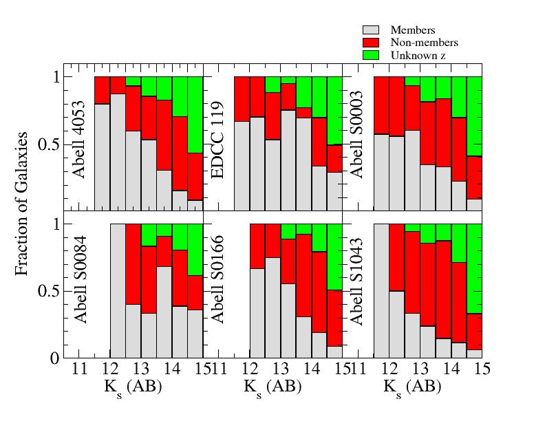
Figure 1: Continued.

In order to create a composite LF we need to correct for incompleteness. Fig. 1 shows the completeness fractions as a function of observed $K$ magnitude for all our clusters, including members, non members and objects for which no redshift is known. In general our spectroscopic completeness is well above 80%, to at least $K\sim 14$. We then correct for incompleteness and produce a composite luminosity function in the same manner as in De Propris et al. (2003). In each magnitude bin, given $N_{C}$ as the number of spectroscopically confirmed cluster members, $N_{R}$ the number of galaxies with redshifts and $N_{I}$ as the total number of objects (including objects with no redshift) we find that the number of galaxies in magnitude bin $j$ of cluster $i$ is given by:

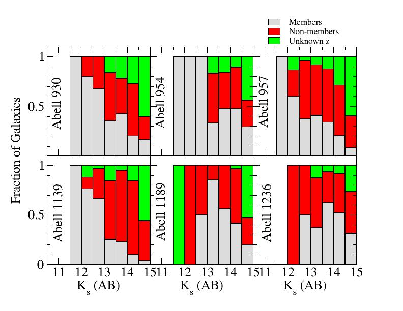
Figure 1: Redshift completeness histograms for a subset of the clusters in our sample (identified in the figure). We show members in grey, non-members in red and objects with unknown redshift in green. See Appendix (online) for all the other clusters in the sample.

$$N_{ij}={N_{C}N_{I}\over N_{R}}$$ (1)

and the corresponding error:

$$\delta N_{ij}=\sqrt{{1\over N_{C}}+{1\over N_{I}}-{1\over N_{R}}}$$ (2)

Following Colless (1989) the composite LF can be calculated by:

$$N_{cj}={N_{c0}\over m_{j}}\sum_{i}{N_{ij}\over N_{i0}}$$ (3)

where $N_{cj}$ is the number of cluster galaxies in magnitude bin $j$, and the sum is carried over the $i$ clusters and $m_{j}$ is the number of clusters contributing to magnitude bin $j$. Here $N_{i0}$ is a normalisation factor, corresponding to the (completeness corrected) number of galaxies brighter than a given magnitude (here we use $K_{s}=13$) in each cluster and

$$N_{c0}=\sum_{i}N_{i0}$$ (4)

The error is then given by:

$$\delta N_{cj}={N_{c0}\over m_{j}}\Bigg{[}\sum_{i}\Bigg{(}{\delta N_{ij}\over N_{ij}}\Bigg{)}^{2}\Bigg{]}^{1/2}$$ (5)

Note that this assumes that the redshift surveys do not select specifically for or against cluster members.

4 Results

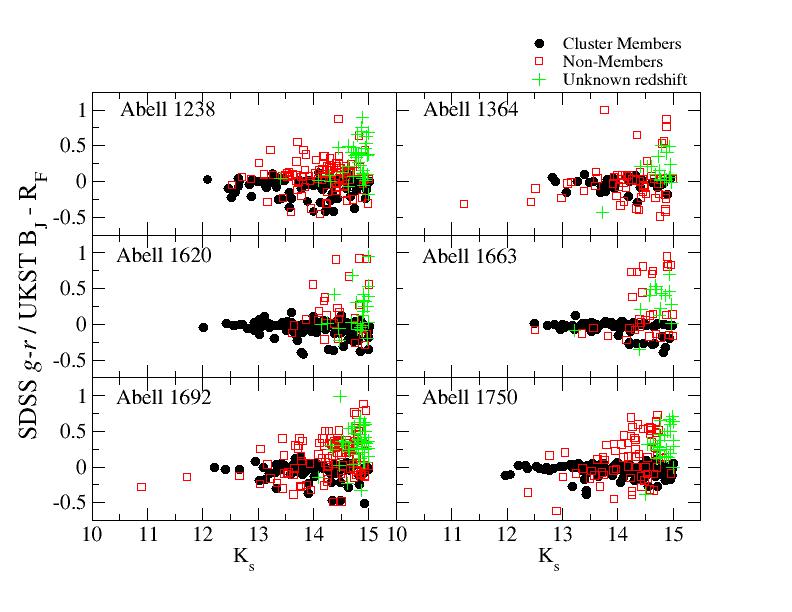
Figure 2: Colour-magnitude diagram for a subset of clusters (members, non-members and unknown redshifts as in the legend). The colours have already been corrected so that the red sequence has 0 colour. See Appendix for all other clusters in the sample

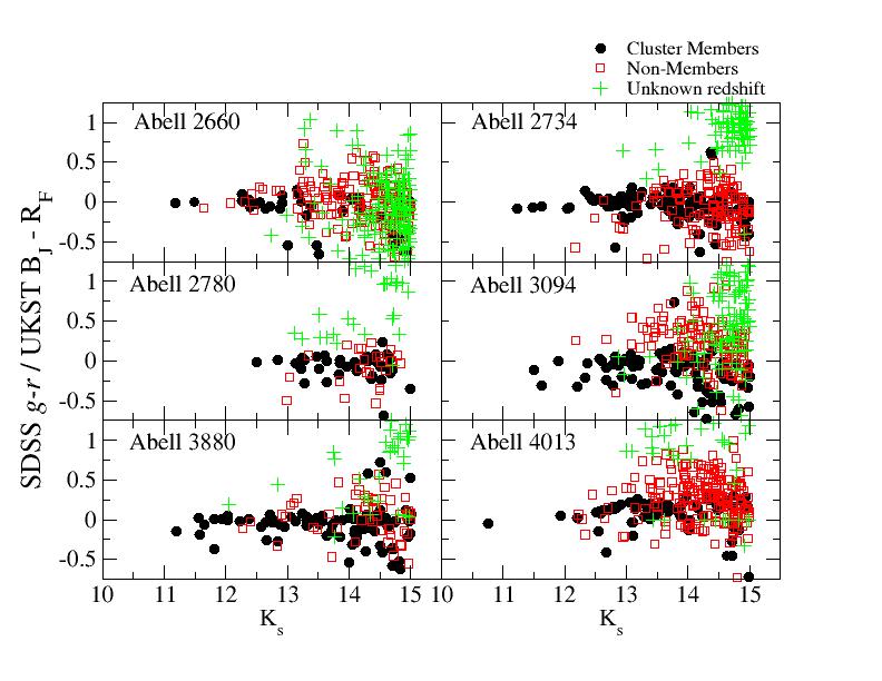
Figure 2: Continued

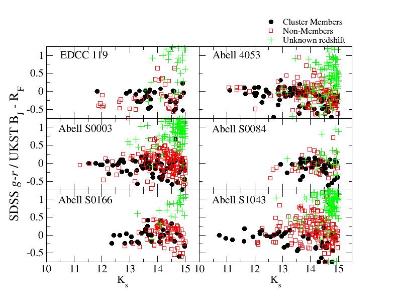
Figure 2: Continued

The best fitting composite $K$-band LF for galaxies in all 24 clusters is shown in Fig. 2, assuming a single Schechter form. The best fitting values are $K^{*}=12.79\ (M_{K}=-24.81)\ \pm 0.14$ and $\alpha=-1.41\pm 0.10$. We also show the associated error ellipse as the errors are correlated.

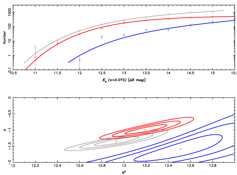
Figure 2: The luminosity functions and best fits to the data for galaxies in all 24 clusters (top panel) with the associated error ellipses (bottom panel). In grey, the total LF, in red the LF for galaxies on the red sequence and in blue the LF for galaxies in the blue cloud. Tables 2 and 3 show the parameter values.

Fig. 3 shows the colour-magnitude relation for galaxies in our clusters, where we have already removed the slope and intercept of the red sequence. Colours come from the SDSS or the UKST as indicated in Table 1 for each cluster. The slope and intercept of the colour-magnitude relation were determined by fitting a minimum absolute deviation straight line to the colour-magnitude relation of cluster members, as this minimizes the effects of interlopers on the fit (Beers et al., 1990). The distribution of colours about the red sequence for all members is shown in Fig  4. (panel (a) for clusters with SDSS data and (b) for clusters with UKST data). The spread at half maximum on the red edge of the distribution is 0.05 mag. for galaxies in clusters with SDSS data ($g-r$) and 0.07 mag. for galaxies in clusters with UKST data ($B_{J}-R_{F}$). We therefore choose to treat galaxies within $\pm 0.15$ and $\pm 0.21$ mag. of the red sequence as red sequence galaxies and the remainder as blue cluster galaxies. Note that in Fig. 3 we have not plotted galaxies redder than the red sequence (as defined above) for clarity.

We then derive a composite LF for red and blue galaxies in all 24 clusters. The red sequence LF and best fit are shown in Fig. 2. This has $K^{*}=13.16$ (–24.44) and $\alpha=-1.00$ (see Table 3). For blue galaxies the Schechter function is a poor fit. The best parameters are $K^{*}=13.51\pm 0.41$ and $\alpha=-1.60\pm 0.29$, albeit with very large errors (see Fig. 2)

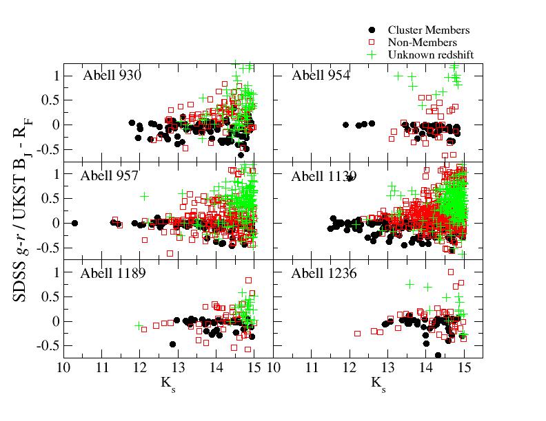
Figure 3: Colour-magnitude diagram for all galaxies in a subsample of clusters (members, non-members and unknown as in the legend). The colours have already been corrected so that the red sequence has 0 colour. Some galaxies lie beyond the axis limits in $y$. See Appendix (online) for all other clusters in the sample

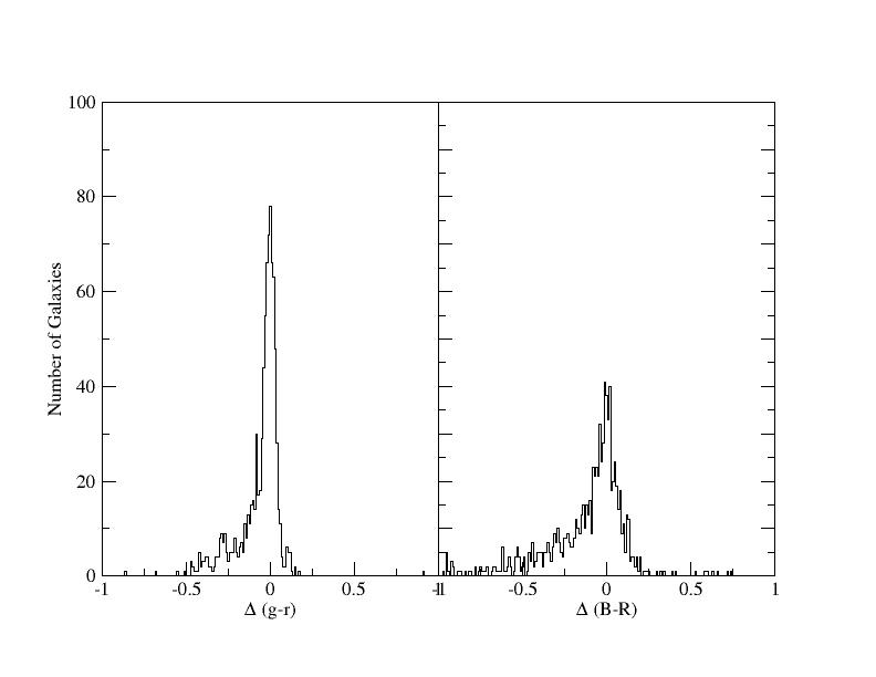
Figure 4: Colour distribution for galaxies about the red sequence, for all 11 clusters with SDSS data (in $g-r$) and 13 clusters with UKST data (in $B_{J}-R_{F}$)

We can also split our sample according to physically significant cluster properties. The velocity dispersion may be taken as an indicator of cluster mass. As in our previous paper (De Propris et al., 2003) we adopt $\sigma=800$ km $s^{-1}$ to separate massive and less massive clusters. We also create samples with Bautz-Morgan type $>II$ and $\leq II$, where the Bautz-Morgan type reflects the relative dominance of the brightest galaxies over the rest of the cluster members and may be an indicator of the degree of dynamical evolution (if the brightest cluster galaxies, for example, grow by dynamical friction and cannibalism). Figure 5 shows the derived LFs and relative error ellipses. Table 2 below shows the values of the derived parameters.

Table 2: $K$ LF parameters

Sample	$K^{*}$	$\alpha$
All	$12.79\pm 0.14$	$-1.41\pm 0.10$
$\sigma<800$ km s-1	$12.83\pm 0.25$	$-1.64\pm 0.13$
$\sigma>800$ km s-1	$12.85\pm 0.18$	$-1.12\pm 0.16$
BM $\leq$ II	$12.79\pm 0.32$	$-1.62\pm 0.19$
BM $>II$	$13.10\pm 0.17$	$-1.40\pm 0.14$

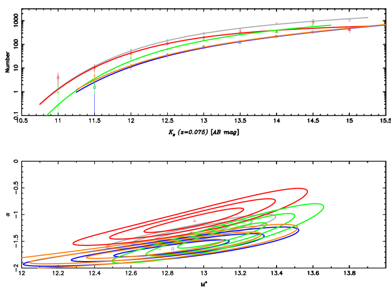
Figure 5: Composite LFs and error ellipses for galaxies in clusters with $\sigma>800$ km s^-1 (blue). $\sigma<800$ km s^-1 (red), BM type $>II$ (green) and BM type $<II$ (orange). The grey line is the total LF for all galaxies.

For red sequence galaxies, we can also consider subsamples of objects, as for the full sample above. This is not possible for the blue cluster members, as there are very few objects in the sample (see Fig. 2). The LFs are shown in Fig. 6 and the relative parameters given in Table 3.

Table 3: Red Sequence $K$ LF parameters

Sample	$K^{*}$	$\alpha$
All	$13.16\pm 0.15$	$-1.00\pm 0.12$
$\sigma<800$ km s-1	$13.30\pm 0.18$	$-0.99\pm 0.14$
$\sigma>800$ km s-1	$13.07\pm 0.24$	$-1.07\pm 0.19$
BM $\leq$ II	$13.16\pm 0.21$	$-1.06\pm 0.17$
BM $>II$	$13.38\pm 0.16$	$-0.81\pm 0.16$

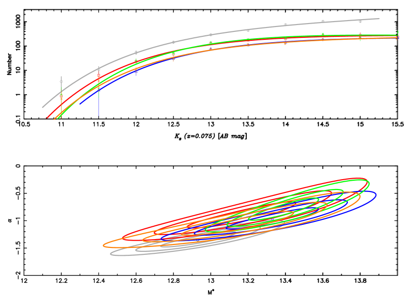
Figure 6: Composite LFs and error ellipses for red sequence galaxies in clusters with $\sigma>800$ km s^-1 (blue), $\sigma<800$ km s^-1 (red), BM type $>II$ (green) and BM type $<II$ (orange). The grey line is the total LF.

5 Discussion

5.1 Comparison with previous work

There are relatively few studies of the $K$-band LF and most of these have been limited to single or small samples of clusters, owing to the small areas of infrared detectors until recently. In the following, we have converted all previous results to the concordance cosmology and to our fiducial redshift $z=0.075$. Our work in Coma (De Propris et al., 1998) may be the closest to the approach we have carried out here, being based on a spectroscopically complete sample of galaxies with $H<14.5$ in the inner $25^{\prime}$ of the Coma cluster. Assuming $H-K=0.2$ mag. for a $\sim K^{*}$ galaxy (Eisenhardt et al., 2007), $K^{*}_{Coma}=13.57$ in De Propris et al. (1998), compared to our value of K${}^{*}=12.79$ in the present study. This is within the $2\sigma$ error ellipse shown in Fig. 2 and closer to the value we determine for red sequence galaxies (that dominate the core of the Coma cluster). Skelton et al. (2009) derive $K^{*}=12.18$, but with a very large error (0.8 mag.) for the Norma cluster. This is still consistent with our measurement. In our previous analysis of 10 2dF clusters (De Propris & Christlein, 2009) we obtained $K^{*}=12.39$ but we have considerably improved our sample, and augmented the redshift completeness, especially at the faint end. Merluzzi et al. (2010), for an ensemble of clusters within the Shapley supercluster, has $K^{*}=12.61$, closer to our value for 24 clusters here. There is considerable variation when comparing with the $K^{*}$ values for single clusters, as the small number statistics at the bright end makes fitting $K^{*}$ difficult. However, our composite LF should provide a better estimate of the LF parameters, as the sparse bright end is more populated. It is not unfortunately not very informative to carry out a comparison between the individual cluster LFs, even with our high completeness, as the errors are so large that there is no statistical power in the analysis.

The faint end slope slope we derive is in good to reasonable agreement with previous studies, especially the estimates by Skelton et al. (2009) for Norma and the Shapley supercluster in Merluzzi et al. (2010). In Coma, the slope is affected by the presence of an inflection in the LF at intermediate magnitudes, but we may remark that there is good agreement with the slope of the LF of red sequence galaxies (Table 2) - nearly all spectroscopically confirmed Coma galaxies in De Propris et al. (1998) are red sequence members. The slope we derive is also steeper than in our previous analysis for a subset of these clusters (De Propris & Christlein, 2009), although the quality of the data has improved, especially at the faint end, which might provide at least part of the explanation for the discrepancy.

5.2 Comparison with the general field

The most recent field $K$-band LF by Jones et al. (2006) has $K^{*}=13.06$ (for our cosmology and at $z=0.075$) and $\alpha=-1.16$, although the fit to a Schechter function is not good. Bell et al. (2003) has $K^{*}=13.60$ and $\alpha=-0.77$, while Cole et al. (2001) has $K^{*}=13.45$ and $\alpha=-0.96$. Despite the differences between these studies, it appears that the cluster $K$ band LF is slightly brighter (by about 30%) and somewhat steeper than in the general field. The brighter LF for cluster galaxies when compared to the field was also found in De Propris et al. (2003), among others, and is understandable if the brighter cluster members are formed from mergers within the cluster environment and/or if the richer cluster environment favours the formation of more massive systems. In order to understand which mechanism is dominant, or even if several such processes are operating, one would need to compare field and cluster LFs as a function of redshift. One caveat to this conclusion is that most previous work has been based on 2MASS photometry. As we have seen above, and as previously found by Andreon (2002) and Kirby et al. (2008), 2MASS magnitudes seem to be $\sim 0.3$ magnitudes fainter, likely because of light losses in the low surface brightness envelopes of galaxies. With this, the difference between field and cluster $K^{*}$ is much reduced and they appear to be identical within the errors. More accurate photometry for wide field surveys is needed to resolve this issue.

The existence of steeper LFs in clusters vs. field galaxies were already pointed out by Merluzzi et al. (2010) for the Shapley supercluster. This steeper slope is somewhat surprising. This may be an environmental effect, although we would expect the field LF to be steeper if the trends we observe in clusters (see below) continue. One possibility is that the 2MASS photometry used by Cole et al. (2001); Bell et al. (2003) and Jones et al. (2006) systematically misses faint galaxies, especially at lower surface brightness levels, and thus leads to a flatter slope than would otherwise be measured (e.g., Andreon 2002; Kirby et al. 2008). Otherwise, one would have to find a mechanism by which dwarfs are preferentially formed or preserved in the theoretically more hostile cluster environments.

5.3 Environmental Effects

We consider the effects of the cluster environment by splitting our sample into several subsamples according to physically significant properties of clusters such as velocity dispersion and the Bautz-Morgan class. We do not find strong evidence that $K^{*}$ varies across these subsamples. This argues that the environment does not strongly affect the behaviour of bright galaxies, at least within clusters.

The only significant difference we find is for the slope of the LF of $\sigma<800$ km s^-1 subsample to be steeper than for the $\sigma>800$ km s^-1 subset, at nearly the $3\sigma$ level (as shown in Fig. 5. For clusters having $\sigma>800$ km s^-1 the LF is flatter than the total LF, while for cluster with $\sigma<800$ km s^-1 it is significantly steeper. We also find that the LF for clusters of BM type $<$ II has also a significantly steeper slope than the total LF and is different from the LF for clusters with BM type $>$ II. The two LFs (for clusters with $<800$ km s^-1 and for clusters with BM type $<II$) are also very similar to each other. Although the two samples do not fully overlap. clusters with BM type $>$ II have slightly larger velocity dispersions than clusters with BM type $\leq$ II.

This may suggest that relatively low mass systems, possibly with a single dominant galaxy, are more favourable to the formation or survival of dwarf galaxies (as in the low density environments of Merluzzi et al. 2010). One possibility is that as clusters grow (from accretion of single galaxies and groups, or mergers with other clusters) the relative dominance of brightest cluster galaxies decreases as more luminous systems are included within the cluster, and as this process takes place dwarfs may be destroyed or captured by more massive galaxies. Here, a single or two massive dominant galaxies in the cluster may be a sign of dynamical youth, rather than evolution. As clusters grow, mergers may become rarer (as the velocity dispersion increases) and the brighter end of the LF may be ‘filled in’ by the infall of bright galaxies.

We have also derived the LF for red sequence galaxies, both for all clusters and for the subsamples we have defined above. The red sequence LF is flatter than the total LF. The red sequence LF does not appear to vary significantly between any of the cluster subsamples. This suggests that any environmental variation is due to the different contributions to the faint end of the LF from blue galaxies. These dominate the low mass end of the LF. We are not able to explore the environmental dependence of the blue LF as the statistics are too poor (the normalisation of the blue LF is about one order of magnitude lower than the red LF). However, the LF slope is similar to that of clusters with $\sigma<800$ km s^-1 and BM type $<$ II. This would suggest that these star-forming dwarf galaxies are preferentially preserved in low mass environments or are destroyed in higher density systems, with many large giants, rather than a single dominant system – it is possible that most of the growth of brightest cluster galaxies may take place outside of clusters - an intriguing parallel may be offered by the ‘infalling’ cD galaxy in the Coma NGC4839 subgroup or the J0454-0309 fossil subgroup (Schirmer et al., 2010).

The actual evolution of the blue galaxies is interesting to consider. Because the red sequence LF is much flatter, they cannot be easily added on to the red sequence (e.g., by quenching). They might fade considerably, and contribute to the steeper faint end observed by (e.g.) Moretti et al. (2015), but one does not expect much fading in $K$, unless they also lose considerable mass (e.g., to tidal stripping). It would be interesting to increase the sample of clusters and obtain deeper spectroscopy.

Merluzzi et al. (2010) found evidence for an environmental dependence on the near-infrared LF in the Shapley supercluster, with the slope of the LF increasing towards lower density regions and being steeper than in the field. We did not find strong evidence that the LF varies radially in our earlier work (De Propris et al., 2003) but the statistics at large ($>300$ kpc) radii were quite small. Adami et al. (2007) suggests that the LF of the Coma cluster steepens along the North-South axis corresponding roughly to the infall direction, while Boue et al. (2008) claim that the LF in Abell 496 steepens towards its outer regions. In Abell 119 Lee et al. (2016) observe a steepening of the LF towards the outer low density regions, together with a more pronounced dip at intermediate luminosities. The trend of the LF to become steeper in bluer bands is well known from several studies (see for instance McNaught-Roberts et al. 2014). This would suggest that most of the “environmental” variation originates from the quenching of low mass galaxies in relatively low density regions, whereas the red sequence members have been largely preprocessed before the epoch of observation (e.g., Gilbank et al. 2008; Zirm et al. 2008). This would explain the observation that the red sequence does not very between our cluster subsamples. Red sequence galaxies are already processed into cluster members in lower density environments.

We can finally compare our findings with the models in Vulcani et al. (2014). For increasing halo mass we see that the $L^{*}$ stellar mass increases by about 30% over two orders of magnitude in halo mass; this is broadly consistent with the field vs. cluster comparison above, but not with the nearly constant $K^{*}$ in all clusters we consider. However, the local field values may be affected by problems with 2MASS photometry. Similarly, the slope is very well matched by the models, but the change in slope with environment is not. As pointed out by Vulcani et al. (2014) the models may still suffer from several shortcomings, especially in the inclusion of cluster-specific environmental effects, the efficiency of galaxy formation and the evolution of central and satellite galaxies.

Appendix A Appendix

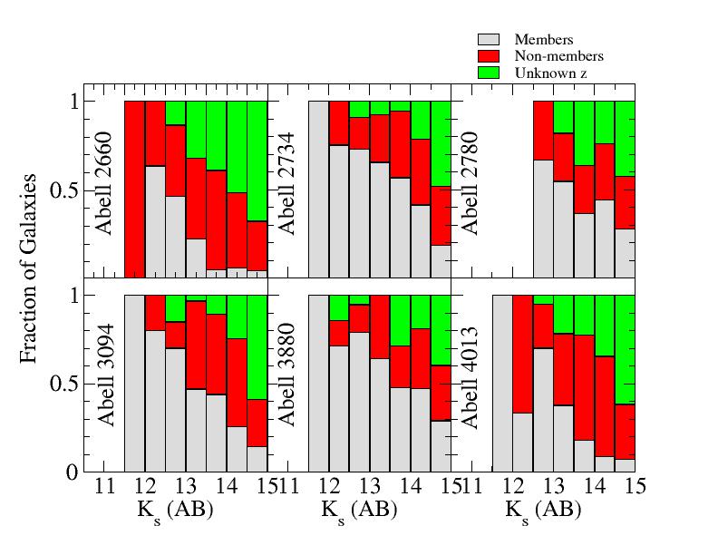
Figure 7: Continued.

References

- Adami et al. (2007) Adami C., Durret F., Mazure A., Pelló R., Picat J. P., West M., Meneux B. 2007, A&A, 462, 411
- Alam et al. (2015) Alam S., Albareti F. D., Allende Prieto C. et al. 2015, ApJS, 219, A12
- Andreon (2002) Andreon S. 2002, A&A, 382, 495
- Autry et al. (2003) Autry, R. G., Probst, R. G., Starr B. M. et al. 2003, Proc. SPIE, 4841, 525
- Babul & Rees (1992) Babul A., Rees M. J. 1992, MNRAS, 255, 346
- Beers et al. (1990) Beers T. C., Flynn K., Gebhardt K. 1990, AJ, 100, 849
- Bell & de Jong (2001) Bell E. F., de Jong R. S. 2001, ApJ, 550, 212
- Bell et al. (2003) Bell E. F., McIntosh D. H., Katz N., Weinberg M. D. 2003, ApJS, 149, 289
- Bertin & Arnouts (1996) Bertin E., Arnouts S. 1996, A&AS, 117, 393
- Blanton et al. (2003) Blanton M. R., Hogg D. W., Bahcall N. A. et al. 2003, ApJ, 592, 819
- Boue et al. (2008) Boue G., Adami C., Durret F., Mamon G. A., Cayatte V. 2008, A&A, 479. 335
- Capozzi et al. (2012) Capozzi D., Collins C. A., Stott J. P., Hilton M. 2012, MNRAS, 419, 2821
- Cole et al. (2001) Cole S., Norberg P., Baugh C. M. et al. 2001, MNRAS, 326, 255
- Colless (1989) Colless M. M. 1989, MNRAS, 237. 799
- Colless et al. (2001) Colless M. M., Dalton G., Maddox S. et al. 2001, MNRAS, 328, 1039
- Contreras et al. (2016) Contreras S., Zehavi I., Baugh C. M., Padilla N., Norberg P. 2016, ArXiv 160706154
- De Propris et al. (1998) De Propris R., Eisenhardt P. R., Stanford S. A., Dickinson M. 1998, ApJ, 503, L45
- De Propris et al. (2002) De Propris R., Couch W. J., Colless M. et al. 2002, MNRAS, 329, 87
- De Propris et al. (2003) De Propris R., Colless M., Driver S. P. et al. 2003, MNRAS, 342, 725
- De Propris & Christlein (2009) De Propris R., Christlieb N. 2009, Astr. Nach. 330, 943
- Eisenhardt et al. (2007) Eisenhardt P., De Propris R., Gonzalez A. H., Stanford S. A., Wang M., Dickinson M. 2007, ApJS, 169, 225
- Eisenstein et al. (2011) Eisenstein D. J., Weinberg D. H., Agol E. et al. 2011, AJ, 142, A72
- Gavazzi et al. (1996) Gavazzi G., Pierini D., Boselli A. 1996, A&A, 312, 297
- Gilbank et al. (2008) Gilbank D. G., Yee H. K. C., Ellingson E., Gladders M. D., Loh Y.-S.. Barrientos L. F., Barkhouse W. A. 2008, ApJ, 673, 742
- Jones et al. (2006) Jones D. H., Peterson B. A., Colless M., Saunders W. 2006, MNRAS, 369, 25
- Kirby et al. (2008) Kirby E., Jerjen H., Ryder S. D., Driver S. P. 2008, AJ, 136, 1866
- Lan et al. (2016) Lan T.-W., Menard B., Mo H. 2016, MNRAS, 459, 3998
- Lee et al. (2016) Lee Y., Rey S.-C., Hilker M., Sheen Y.-K., Yi S. K. 2016, ApJ, 822, A92
- McNaught-Roberts et al. (2014) McNaught-Roberts T., Norberg P., Baugh C. et al. 2014, MNRAS, 445, 2125
- Merluzzi et al. (2010) Merluzzi P., Mercurio A., Haines C. P., Smith R. J., Busarello G., Lucey J. R. 2010, MNRAS, 402, 753
- Moretti et al. (2015) Moretti A., Bettoni D., Poggianti B. M. et al. 2015 A&A, 581, A11
- Narayanan (2016) Narayanan D. 2016, Nature Physics, 12, 636
- Probst et al. (2003) Probst R. G., Montane A., Warner M. et al. 2003, Proc. SPIE, 4841, 411
- Rines & Geller (2008) Rines K. & Geller M. J. 2008, AJ, 135, 1837
- Rudnick et al. (2009) Rudnick G., von der Linder A., Pelló R. et al. 2009, ApJ, 700, 1559
- Sanchez-Janssen et al. (2016) Sanchez-Janssen R., Ferrarese L., MacArthur L. A. et al. 2016, ApJ, 820, A69
- Schirmer et al. (2010) Schirmer M., Suyu S., Schrabback T., Hildebrandt H., Erben T., Halkola A. 2010, A&A, 514, A60
- Skelton et al. (2009) Skelton R. E., Woudt P. A., Kraan-Korteweg R. C. 2009, MNRAS, 396, 2367
- Skrutskie et al. (2006) Skrutskie M. F., Cutri R. M., Stiening R. et al. 2006, AJ, 131, 1163
- Swaters et al. (2009) Swaters R. A., Valdes F., Dickinson M. E. 2009, in ADASS XVIII, ASP Conf. ser. 411, p. 506
- Vulcani et al. (2014) Vulcani B., De Lucia G., Poggianti B. M., Bundy K., More S., Calvi R. 2014, ApJ, 788, A57
- York et al. (2000) York D. G., Adelman J., Anderson J. E. et al. 2000, AJ, 120, 1579
- Zabludoff et al. (1990) Zabludoff A. I, Huchra J. P., Geller M. 1990, ApJS, 74, 1
- Zhang & Bell (2016) Zhang Y., Bell E. F. 2016, arXiv 1610.06174
- Zirm et al. (2008) Zirm A. W., Stanford S. A., Postman M. et al. 2008, ApJ, 680, 224