Enhancement of the $d$-wave pairing correlations by charge and spin ordering in the spin-one-half Falicov-Kimball model with Hund and Hubbard coupling

Abstract

Projector Quantum-Monte-Carlo Method is used to examine effects of the spin-independent $U_{fd}$ as well as spin-dependent $J_{z}$ Coulomb interaction between the localized $f$ and itinerant $d$ electrons on the stability of various types of charge/spin ordering and superconducting correlations in the spin-one-half Falicov-Kimball model with Hund and Hubbard coupling. The model is studied for a wide range of $f$ and $d$-electron concentrations and it is found that the interband interactions $U_{fd}$ and $J_{z}$ stabilize three basic types of charge/spin ordering, and namely, (i) the axial striped phases, (ii) the regular $n$-molecular phases and (iii) the phase separated states. It is shown that the $d$-wave pairing correlations are enhanced within the axial striped and phase separated states, but not in the regular phases. Moreover, it was found that the antiferromagnetic spin arrangement within the chains further enhances the $d$-wave paring correlations, while the ferromagnetic one has a fully opposite effect.

PACS nrs.: 71.27.+a, 71.28.+d, 74.20.-z

1 Introduction

In the past decades, a considerable amount of effort has been devoted to understand a formation of an inhomogeneous charge and spin stripe order in strongly correlated electron systems as well as its relation to superconductivity. The motivation was clearly due to the observation of such an ordering in doped nickelate [1], cuprate [2] and cobaltate [3] materials, some of which constitute materials that exhibit high-temperature superconductivity. The Hubbard and $t-J$ models have been used the most frequently in the literature to study the problem of stripe formation [4, 5]. These studies showed on two possible explanations of formation of inhomogeneous spatial charge and spin ordering. According to the first explanation the stripe phases arise from a competition between the tendency to phase separate (the natural tendency of the system) and the long-range Coulomb interaction [6]. Contrary to this explanation, White and Scalapino proposed [5] a new mechanism that does not require the long-range interactions and according to which the stripe order arises from a competition between kinetic and exchange energies. Much simpler mechanism of a charge stripe formation in strongly correlated systems has been found by Lemanski et al. [7] within the spinless Falicov-Kimball model (FKM). This model [8] combines only the kinetic energy of itinerant $d$ electrons with the on-site Coulomb interaction between the itinerant $d$ and localized $f$ electrons and thus various types of charge orderings determined within this model for different $f$ and $d$ electron dopings are simply a compromise between these two tendencies.

However, the spinless version of the FKM, although non-trivial, is not able to account for all aspects of real experiments. For example, many experiments show that a charge superstructure is accompanied by a magnetic superstructure [1, 2]. In order to describe both types of ordering in the unified picture Lemanski [9] proposed a simple model based on a generalization of the spin-one-half FKM that besides the local Coulomb interaction between $f$ and $d$ electrons takes into account also the anisotropic, spin-dependent local interaction (of the Ising type) that couples the localized and itinerant subsystems. It was found that this model is able to describe various types of charge and spin orderings observed experimentally in strongly correlated systems, including the diagonal and axial charge stripes with antiferromagnetic or ferromagnetic arrangement of spins within the lines.

In spite of this fact, the extended model is still oversimplified to describe all details of real materials. The major simplification consists of omitting the Hubbard interaction $U_{dd}$ between the itinerant electrons of opposite spins that is crucial if one interests, for example, in the superconducting correlations in the system. Since the main goal of this paper is to examine the impact of charge and spin superstructures on the superconducting correlations we have extended the Lemanski’s model by the Hubbard interaction term. From this point of view, the model considered here, for a description of superconducting correlations in the strongly correlated system, is the spin-one-half FKM extended by the anisotropic spin-dependent interband interaction of the Ising type (between $f$ and $d$ electrons) and the intraband Coulomb interaction of the Hubbard type that acts between two $d$ ($f$) electrons of opposite spins.

It should be noted that despite an enormous research activity in the past the relation between the charge/spin ordering and the superconductivity is still controversial (an excellent review of relevant works dealing with this subject can be found in [10]). A considerable progress in this field has been achieved recently by Maier et al. [11] and Mondaini et al. [12]. Both groups studied the two-dimensional Hubbard model, in which stripes are introduced externally by applying a spatially varying local potential $V_{i}$, and they found a significant enhancement of the d-wave pairing correlations. However, it should be noted that the potential $V_{i}$ is phenomenological and as such has no direct microscopic origin that corresponds to a degree of freedom in the actual materials. The advantage of our approach, based on the generalized spin-one-half FKM with $U_{fd}$, $J_{z}$ and $U_{dd}$ interactions is that the charge/spin stripes are present in the model intrinsically, even in its $U_{dd}=0$ limit.

2 Model

The Hamiltonian of the model considered in this paper has the form

$$H = -t\sum_{\langle i,j\rangle\sigma}d^{+}_{i\sigma}d_{j\sigma}+U_{fd}\sum_{i\sigma\sigma^{\prime}}f^{+}_{i\sigma}f_{i\sigma}d^{+}_{i\sigma^{\prime}}d_{i\sigma^{\prime}}+J_{z}\sum_{i\sigma}(f^{+}_{i-\sigma}f_{i-\sigma}-f^{+}_{i\sigma}f_{i\sigma})d^{+}_{i\sigma}d_{i\sigma}$$ (1)

$$+ U_{dd}\sum_{i}d^{+}_{i\uparrow}d_{i\uparrow}d^{+}_{i\downarrow}d_{i\downarrow}\ ,$$

where $f^{+}_{i\sigma},f_{i\sigma}$ are the creation and annihilation operators for an electron of spin $\sigma=\uparrow,\downarrow$ in the localized state at lattice site $i$ and $d^{+}_{i\sigma},d_{i\sigma}$ are the creation and annihilation operators of the itinerant electrons in the $d$-band Wannier state at site $i$.

The first term of (1) is the kinetic energy corresponding to quantum-mechanical hopping of the itinerant $d$ electrons between sites $i$ and $j$. These intersite hopping transitions are described by the matrix elements $t_{ij}$, which are $-t$ if $i$ and $j$ are the nearest neighbours and zero otherwise. The second term represents the on-site Coulomb interaction between the $d$-band electrons with density $n_{d}=N_{d}/L=\frac{1}{L}\sum_{i\sigma}d^{+}_{i\sigma}d_{i\sigma}$ and the localized $f$ electrons with density $n_{f}=N_{f}/L=\frac{1}{L}\sum_{i\sigma}f^{+}_{i\sigma}f_{i\sigma}$, where $L$ is the number of lattice sites. The third term is the above mentioned anisotropic, spin-dependent local interaction of the Ising type between the localized and itinerant electrons that reflects the Hund’s rule force. And finally, the last term is the ordinary Hubbard interaction term for the itinerant electrons from the $d$ band. Moreover, it is assumed that the on-site Coulomb interaction between $f$ electrons is infinite and so the double occupancy of $f$ orbitals is forbidden.

This model has several different physical interpretations that depends on its application. As was already mentioned above, it can be considered as the spin-one-half FKM extended by the Hund and Hubbard interaction term. On the other hand, it can be also considered as the Hubbard model in the external potential generated by the spin-independent Falicov-Kimball term and the anisotropic spin-dependent Hund term. Very popular interpretation of the model Hamiltonian (1) is its $(U_{dd}=0)$ version that has been introduced by Lemanski [9] who considered it as the minimal model of charge and magnetic ordering in coupled electron and spin systems. Its attraction consists in this that without the Hubbard interaction term $(U_{dd}=0)$ the Hamiltonian (1) can be reduced to the single particle Hamiltonian. Indeed, using the fact that the $f$-electron occupation number $f^{+}_{i\sigma}f_{i\sigma}$ of each site $i$ commutes with the Hamiltonian (1), it can be replaced by the classical variable $w_{i\sigma}$ taking only two values: $w_{i\sigma}=1$ or 0, according to whether or not the site $i$ is occupied by the localized $f$ electron and so the Hamiltonian (1) in absence of $U_{dd}$ term can be written as

$$H=\sum_{ij\sigma}h^{(\nu)}_{ij}d^{+}_{i\sigma}d_{j\sigma},$$ (2)

where $h^{(\nu)}_{ij}=t_{ij}+(U_{fd}w_{i}+J_{z}\nu{s_{i}})\delta_{ij}$, $w_{i}=w_{i\uparrow}+w_{i\downarrow}=0,1$, $s_{i}=w_{i\uparrow}-w_{i\downarrow}=-1,1$ (we remember that the double occupancy of $f$ orbitals is forbidden) and $\nu=\pm 1$. Thus for a given $f$-electron $w=\{w_{1},w_{2},\dots,w_{L}\}$ and spin configuration $s=\{s_{1},s_{2},\dots,s_{L}\}$ the investigation of the model (2) is reduced to the investigation of the spectrum of $h^{(\nu)}$ for different $f$ electron/spin distributions. This can be performed exactly, over the full set of $f$-electron/spin distributions or approximatively. One such approximative method has been introduced in our previous papers [13, 14] and it was shown that it is very effective in description of ground-state properties of the model Hamiltonian (2) and its extensions. The method consists of the following steps: i) Chose a trial configuration $c=\{w;s\}$. (ii) Having $U_{fd}$, $J_{z}$ and the total number of electrons $N=N_{f}+N_{d}$ fixed, find all eigenvalues $\lambda^{(\nu)}_{k}$ of $h^{(\nu)}$. (iii) For a given $N_{f}=\sum_{i}w_{i}$ determine the ground-state energy $E(c)$ of a particular $f$-electron/spin configuration by filling in the lowest $N_{d}=L-N_{f}$ one-electron levels $\lambda^{(\nu)}_{k}$. (iv) Generate a new configuration $c^{\prime}$ by moving a randomly chosen electron to a new position which is chosen also as random (or equivalently by flipping the randomly chosen spin). (v) Calculate the ground-state energy $E(c^{\prime})$. If $E(c^{\prime})<E(c)$ the new configuration is accepted, otherwise $c^{\prime}$ is rejected. Then the steps (ii)-(v) are repeated until the convergence (for given $U_{fd}$ and $J_{z}$ ) is reached. Of course, one can move (flip) instead of one electron in step (iv) simultaneously two or more electrons (spins), thereby the convergence of method is improved. For the $U_{dd}>0$ case studied in the current paper we use the quantum variant of this method, that differs from the classical one only in the step (iii) where the ground state energy of the full Hamiltonian (1) has to be calculated now by a quantum method. Here we used the exact diagonalization Lanczos method [15] for clusters less than $L=16$ sites and the Projector Quantum Monte Carlo method [16] for larger clusters.

Having the actual charge and spin distributions that minimize the ground state energy of the model Hamiltonian (1) all ground state observables can be calculated immediately. In the current paper we focus our attention to the problem of superconducting correlations in the ground state. Especially we study the influence of the spin-independent Coulomb interaction $U_{fd}$ (the charge ordering) and the anisotropic spin-dependent interaction $J_{z}$ (the spin ordering) on the superconducting correlation function with $d_{x^{2}-y^{2}}$ wave symmetry defined as [17]

$$C_{d}(r)=\frac{1}{L}\sum_{i,\delta,\delta^{\prime}}g_{\delta}g_{\delta^{\prime}}\langle d^{+}_{i\uparrow}d^{+}_{i+\delta\downarrow}d_{i+\delta^{\prime}+r\downarrow}d_{i+r\uparrow}\rangle,$$ (3)

where the factors $g_{\delta},g_{\delta^{\prime}}$ are 1 in x-direction and -1 in y-direction and the sums with respect to $\delta,\delta^{\prime}$ are independent sums over the nearest neighbors of site $i$.

However, on small clusters the above defined correlation function is not a good measure for superconducting correlations, since contains also contributions from the one particle correlation functions

$$C^{\sigma}_{0}(r)=\frac{1}{L}\sum_{i}\langle d^{+}_{i\sigma}d_{i+r\sigma}\rangle,$$ (4)

that yield nonzero contributions to $C_{d}(r)$ even in the noninteracting case.

For this reason we use as the true measure for superconductivity the vertex correlation function

$$C^{v}_{d}(r)=C_{d}(r)-\sum_{\delta,\delta^{\prime}}g_{\delta}g_{\delta^{\prime}}C^{\uparrow}_{0}(r)C^{\downarrow}_{0}(r+\delta-\delta^{\prime})\rangle,$$ (5)

and its average

$$C^{v}_{d}=\frac{1}{L}\sum_{i}C^{v}_{d}(i).$$ (6)

3 Results and discussion

We have started our study with the case $J_{z}=0$, that is slightly simpler from the numerical point of view, since in this case it is necessary to work only with the charge degrees of freedom. Unlike previous studies [9, 18, 19, 20], that have been done exclusively for $U_{dd}=0$, we consider here also the Hubbard interaction term with the intraband Coulomb interacting $U_{dd}=2$. To reveal effects of the interband Coulomb interaction between localized and itinerant electrons $U_{fd}$ on the formation of the various types of charge ordering, we have analyzed model for a wide range of $U_{fd}$ values ($U_{fd}=0,0,5,1,2,3\dots 8$) at all possible combinations of half and quarter $f$ and $d$ electron fillings on cluster of $L=8\times 8$ sites. The results of our numerical calculations obtained within the method described in detail above are summarized in Fig. 1. There is displayed the complete list of $f$-electron configurations that minimize ground state energy of the model for different values of $U_{fd},n_{f}$ and $n_{d}$.

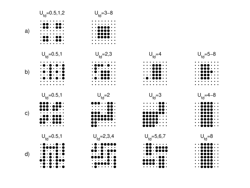
Figure 1: Ground states of the model (1) calculated for $U_{dd}=2,J_{z}=0,L=8\times 8$ at different values of the interband Coulomb interaction $U_{fd}$ and different $f$ and $d$ electron filings: a) $n_{f}=1/4,n_{d}=1/4$; b) $n_{f}=1/4,n_{d}=1/2$; c) $n_{f}=1/2,n_{d}=1/4$; d) $n_{f}=1/2,n_{d}=1/2$. Here the dark circles represent the $f$ electrons and dots the empty sites.

Analysing these results one can see some general trends in formation of charge ordering. For sufficiently large $U_{fd}$ there is an obvious tendency to the phase separation for all examined $f$ and $d$ electron fillings, while in the opposite limit there is a tendency to form the axial stripes (for $n_{f}=1/4,n_{d}=1/2$ and $n_{f}=1/2,n_{d}=1/2$) or regularly distributed ”n-molecules” of $f$-electrons for ($n_{f}=1/4,n_{d}=1/4$ and $n_{f}=1/2,n_{d}=1/4$). Between these three basic types of ground state configurations there is a limited number of intermediate phases through which the low $U_{fd}$ phases transform to high $U_{fd}$ ones.

Of course, the charge ordering in the $f$-electron subsystem will have the strong impact on the $d$ electrons. To show what happens with the $d$ electrons we have calculated directly the $d$-electron on-site occupation $n_{i}=\sum_{\sigma}\langle d^{+}_{i\sigma}d_{i\sigma}\rangle$ for several representative $f$-electron distributions from Fig. 1, including the regular, phase separated and axial striped phases.

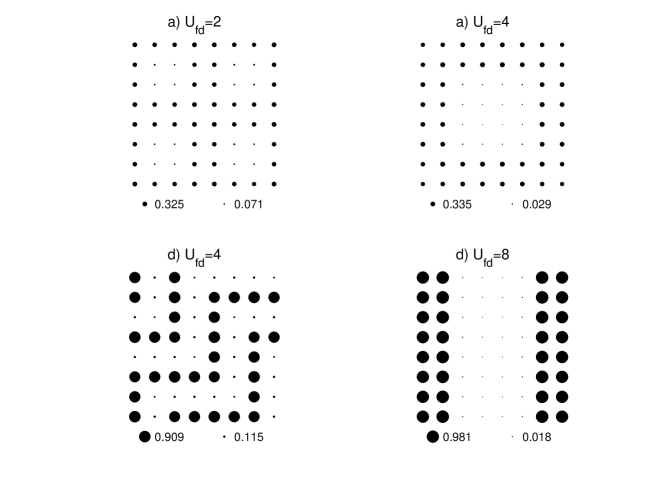
Figure 2: The $d$-electron on-site occupation $n_{i}=\sum_{\sigma}\langle d^{+}_{i\sigma}d_{i\sigma}\rangle$ calculated for selected $f$-electron configurations from Fig. 1. The case a) corresponds to $n_{f}=1/4,n_{d}=1/4$ and the case d) to $n_{f}=1/2,n_{d}=1/2$. The on-site occupation $n_{i}$ is represented by filled-circles ($\bullet$), where the radius of circle on site $i$ is proportional to $n_{i}$.

It is seen (see Fig. 2) that $d$ and $f$ electrons exhibit the inverse site occupancy, which is obviously a consequence of the local Coulomb interaction $U_{fd}$ that prefers states without double $d$-$f$ site occupancy. As a result, the majority of $d$ electrons reside on the empty sites and only a fraction of them (due to the quantum mechanical hopping) share the same sites with $f$ electrons. This leads not only to the inverse $f$ and $d$ site occupancy, but also to the inverse charge patterns in the $f$ and $d$ electron subsystems and thus the axial stripes (the phase separation) in the $f$ electron subsystem are accompanied by the axial stripes (the phase separation) in the $d$-electron subsystem.

The average vertex correlation functions corresponding to the ground state configurations from Fig. 1 are displayed in Fig. 3. Let us now discuss different cases in detail.

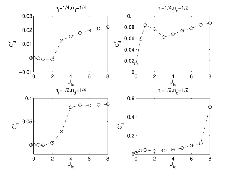
Figure 3: Average vertex correlation function $C^{v}_{d}$ with $d_{x^{2}-y^{2}}$-wave symmetry as a function of the interband Coulomb interaction $U_{fd}$ calculated for corresponding ground states from Fig. 1.

For $n_{f}=1/4,n_{d}=1/4$ the average vertex correlation function exhibits extremely different behaviour in regions of stability of the regular phase with the 4-molecules and the phase separated ground state. While in the first case, the correlation function is small and with increasing $U_{fd}$ changes only slowly, in the second case it is significantly enhanced at the phase boundary and further increases with increasing $U_{fd}$. A fully different picture is observed for $n_{f}=1/4,n_{d}=1/2$. Here the average vertex correlation function sharply increases with increasing $U_{fd}$ within the axial striped phase, then slowly decreases within the intermediate phases and it is again enhanced in the phase separated region. For $n_{f}=1/2,n_{d}=1/4$ the system exhibits a similar behaviour as for $n_{f}=1/4,n_{d}=1/4$ with an exception that the vertex correlations in the separated phase are now four times larger than in the $n_{f}=1/4,n_{d}=1/4$ case. In the last case $n_{f}=1/2,n_{d}=1/2$ the average vertex correlation function changes slowly for both the axial striped as well regular phase, but it is enhanced dramatically in the separated phase. This enhancement is by the factor 6, in comparison to the $n_{f}=1/4,n_{d}=1/2$ and $n_{f}=1/2,n_{d}=1/4$ phases and even by the factor 25 for the $n_{f}=1/4,n_{d}=1/4$ phase, what emphasizes the role of $f$ ($d$) electron doping on the superconducting correlations.

Thus we can conclude that the separated and axial striped phases enhance the average vertex correlations in the spin-one-half FKM with $U_{fd},J_{z}$ and $U_{dd}$ couplings, while the regular phases have only a small impact on the $d_{x^{2}-y^{2}}$ superconducting correlations in this model. Unfortunately, for half and quarter $f$ and $d$ electron fillings analysed above we have found no pure axial striped phases, as observed in the experiments for some cuprate, nikelate and cobaltate systems and therefore we turn our attention to the case $n_{f}+n_{d}=1$ and $n_{f}+n_{d}=2$, where such phases have been widely observed for both $J_{z}=0$ as well as $J_{z}>0$, even in the limit $U_{dd}=0$. [19]

The results of our nonzero $U_{dd}$ calculations are presented in Fig. 4 for $U_{dd}=2,U_{fd}=4$ and $J_{z}=0.5$. Comparing these results with ones obtained in our previous paper [19] for $U_{dd}=0$, and the same values of $U_{fd}$ and $J_{z}$, one can see that they are identical practically for all examined $f$ electron concentrations for both $n=1$ and $n=2$.

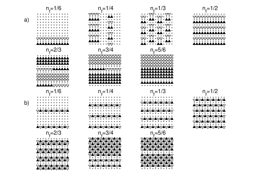
Figure 4: Ground states of the model (1) calculated for $U_{dd}=2,U_{fd}=4,J_{z}=0.5,L=12\times 12$ and different values of the $f$-electron concentrations at (a) $n=n_{f}+n_{d}=1$ and (b) $n=n_{f}+n_{d}=2$. Here the spin up (down) of the $f$ electron is represented by a filled regular triangle (open inverted triangle).

The exceptions have been observed only for $n_{f}=1/4$ and $n_{f}=2/3$ ($n=1$), where slightly different types of the ground states have been identified for $U_{dd}=0$ and $U_{dd}>0$. This independently confirms the supposition made in our previous papers [18, 19], based on the small cluster exact diagonalization calculations, and namely that in the strong interaction $U_{fd}$ limit ($U_{fd}\geq 4$), the ground states of the model found for $U_{dd}=0$ persist as ground states also for nonzero $U_{dd}$, up to relatively large values ($U_{dd}\sim 3$).

Let us now summarize our numerical results for the ground states. (i) In all examined cases the ground states of the model (1) are non-polarized ($n_{f\uparrow}=n_{f\downarrow}$, $n_{d\uparrow}=n_{d\downarrow}$) for both the $n_{f}+n_{d}=1$ as well as $n_{f}+n_{d}=2$ line. (ii) For $n_{f}+n_{d}=1$ the ground states are either the regular distributions of $f$ electrons ($n_{f}=1/3$) or the axial striped configurations, some of which can be phase separated ($n_{f}=1/6$ and $n_{f}=5/6$). (iii) For $n_{f}+n_{d}=2$ only the axial striped configurations are the ground states of the model, and the phase separation is observed only for $n_{f}=3/4$.

The average vertex correlation functions calculated for a complete list of ground state configurations from Fig. 4 are shown in Fig. 5 ($n=1$) and Fig. 6 ($n=2$). To see the enhancement of superconducting correlations due to the interband Coulomb $U_{fd}$ and spin $J_{z}$ interaction against the ordinary Hubbard model with $U_{dd}=2$ we have plotted $C^{v}_{d}$ for both $U_{fd}=4,J_{z}=0.5$ and $U_{fd}=0,J_{z}=0$.

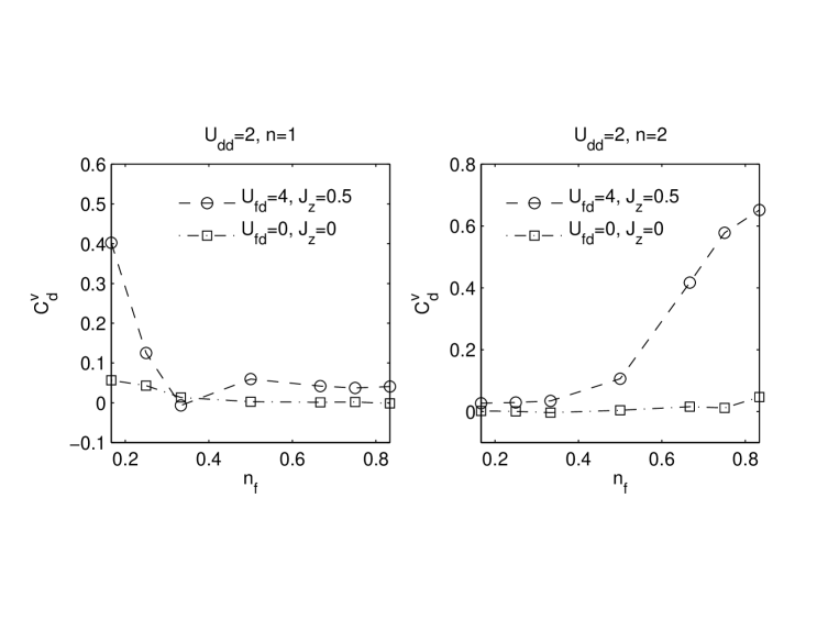
Figure 5: Average vertex correlation function $C^{v}_{d}$ as a function of $n_{f}$ calculated for corresponding ground states from Fig. 4 at $U_{fd}=4,J_{z}=0.5$ (the dashed line) and $U_{fd}=0,J_{z}=0$ (the dash-dotted line).

One can see that the superconducting correlations for $n=1$ are considerably enhanced for $n_{f}=1/6,1/4,1/2,2/3,3/4$ and $5/6$, while they are practically unchanged for $n_{f}=1/3$. The ground state configurations for $n_{f}=1/6,1/4,1/2,3/4$ and $5/6$ are either phase separated or axially striped and thus the enhancement of superconducting correlations in these phases is in accordance with our results discussed above for half and quarter $f$ and $d$ electron fillings. In accordance with these conclusions, it is also the result obtained for $n_{f}=1/3$. In this case the pairs of $f$-electrons are distributed regularly over the whole two-dimensional lattice and thus the suppression of superconducting correlations is expected.

A fully different picture is observed for $n=2$, where the superconducting correlations are enhanced for all examined values of $f$-electron concentrations and they sharply increase with $f$-electron doping (for example, for $n_{f}=5/6$ they are enhanced by a factor 20 in comparison to the $U_{fd}=0$ and $J_{z}=0$ case). For all examined $n_{f}$ the ground states are the axially striped phases and thus these results are also consistent with our above mentioned conclusions.

To separate contributions to $C^{v}_{d}$ from $U_{fd}$ and $J_{z}$ we have plotted in Fig. 6 the average vertex correlation function $C^{v}_{d}$ as a function of $n_{f}$ for $J_{z}=0.5$ as well as $J_{z}=0$.

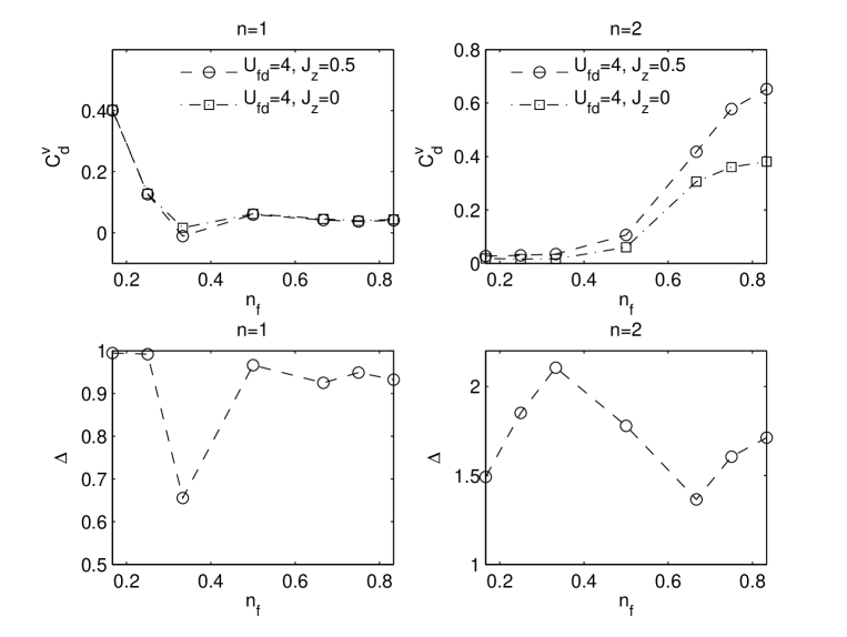
Figure 6: Average vertex correlation function $C^{v}_{d}$ as a function of $n_{f}$ calculated for corresponding ground states from Fig. 4 at $U_{fd}=4,J_{z}=0.5$ (the dashed line) and $U_{fd}=4,J_{z}=0$ (the dash-dotted line) for both $n=1$ and $n=2$. The enhancement $\Delta$ corresponds to the ratio of the average vertex correlation functions with and without the Ising coupling $J_{z}$, $\Delta=C^{v}_{d}(U_{fd}=4,J_{z}=0.5)/C^{v}_{d}(U_{fd}=4,J_{z}=0)$.

It is seen that the Hund constant suppresses the superconducting correlations for $n=1$, the most obviously for $n_{f}=1/3$, while in the case $n=2$ the nonzero $J_{z}$ enhances considerably superconducting correlations. Comparing the types of spin arrangement within the axial phases for $n=1$ and $n=2$, the reason for such a different behaviour seems to be obvious. While for $n=1$ the spins are arranged ferromagnetically within the individual lines, for $n=2$ they are arranged antiferromagnetically. This implies that the antiferromagnetic correlations within the axial stripes enhance the superconducting correlations in the $d_{x^{2}-y^{2}}$ channel, while the ferromagnetic ones has the opposite effect.

In summary, the Projector Quantum Monte Carlo Method is used to examine effects of the interband Coulomb interaction $U_{fd}$ and the anisotropic spin-dependent interband interaction $J_{z}$ on the stability of various types of charge/spin ordering and superconducting correlations in the two-dimensional spin-one-half FKM with Hund and Hubbard coupling. It is found that for half and quarter $f$ and $d$ electron fillings the intraband Coulomb interaction $U_{fd}$ stabilized the axial striped or regular $n$-molecular phases for small and intermediate values of $U_{fd}$ and the phase separated $f$-electron distributions for $U_{fd}$ large. The superconducting vertex correlation functions were strongly enhanced within the axial striped and phase separated states, while they were small within the regular $n$-molecular phases. Along the lines $n_{f}+n_{d}=1$ and $n_{f}+n_{d}=2$ only the axial striped or $n$-molecular charge phase were identified. For $n=1$ the $d$-wave correlations were enhanced for axial striped phases (with $n_{f}=1/6,1/4,1/2,3/4,5/6$) and suppressed for the periodic $n_{f}=1/3$ phase. Unlike this case, for $n=2$ the $d$-wave vertex correlations were enhanced for all examined $f$-electron fillings and the most significantly for $n_{f}\to 1$. Moreover, it was found that the superconducting correlations in the axial striped phases were strongly influenced by spin arrangements within lines. In particular, the antiferromagnetic spin arrangement (found for $n=2$) further enhances the d-wave paring correlations, while the ferromagnetic spin arrangement (found for $n=1$) has the opposite effect.

This work was supported by Slovak Research and Development Agency (APVV) under Grant APVV-0097-12 and ERDF EU Grants under the contract No. ITMS 26220120005 and ITMS26210120002.

References

- [1] C. H. Chen, S.-W. Cheong and A. S. Cooper, Phys. Rev. Lett. 71, 2461 (1993); J. M. Tranquada, D. J. Buttrey, V. Sachan and J. E. Lorenzo, Phys. Rev. Lett. 73, 1003 (1994); Phys. Rev. B 52, 3581 (1995); V. Sachan et al., ibid. 51, 12742 (1995).
- [2] J. M. Tranquada, B. J. Sternlieb, J. D. Axe, Y. Nakamura and S. Uchida, Nature (London) 375, 561 (1995); Phys. Rev. B 54, 7489 (1996); Phys. Rev. Lett. 78, 338 (1997); H. A. Mook, P. Dai and F. Dogan, Phys. Rev. Lett. 88, 097004 (2002);
- [3] K. Takada, H. Sakurai, E. Takayama-Muromachi, F. Izumi, R. Dilanian, and T. Sasaki, Nature (London) 422, 53 (2003)
- [4] A. M. Oles, Acta Phys. Pol. B 31, 2963 (2000).
- [5] S. R. White and D. J. Scalapino, Phys. Rev. Lett. 80, 1272 (1998).
- [6] V. J. Emery, S. A. Kivelson, and H. Q. Lin, Phys. Rev. Lett. 64, 475 (1990).
- [7] R. Lemanski, J. K. Freericks and G. Banach, Phys. Rev. Lett. 89, 196403 (2002);
- [8] L.M. Falicov and J.C. Kimball, Phys. Rev. Lett. 22, 997 (1969).
- [9] R. Lemanski, Phys. Rev. B 71, 035107 (2005).
- [10] A.M. Oles, Acta Physica Polonica B 121, 752 (2012).
- [11] T.A. Maier, G. Alvarez, M. Summers and T.C. Schulthess, Phys. Rev. Lett. 104, 247001 (2010).
- [12] R. Mondaini, T. Ying, T. Paiva and R.T. Scalettar, Phys. Rev. B 86, 184506 (2012).
- [13] P. Farkašovský, Eur. Phys. J. B 20, 209 (2001).
- [14] H. Čenčariková and P. Farkašovský, Int. J. Mod. Phys. B18, 357 (2004).
- [15] E. Dagotto, Rev. Mod. Phys. 66, 763 (1994).
- [16] M. Imada and Y. Hatsugai, J. Phys. Soc. Jpn. 58, 3752 (1989).
- [17] M. Fettes, I. Morgenstern and T. Husslein, Computer Physics Communications 106, 1 (1997).
- [18] P. Farkašovský and H. Čenčariková, Eur. Phys. J. B 47, 517 (2005).
- [19] H. Čenčariková and P. Farkašovský, phys. stat. sol. (b) 245, 2593 (2008).
- [20] R. Lemanski and J. Wrzodak, Phys. Rev. B 78, 085118 (2008).