The Asset Liability Management problem of a nuclear operator : a numerical stochastic optimization approach.

Abstract

We numerically study an Asset Liability Management problem linked to the decommissioning of French nuclear power plants. We link the risk aversion of practitioners to an optimization problem. Using different price models we show that the optimal solution is linked to a de-risking management strategy similar to a concave strategy and we propose an effective heuristic to simulate the underlying optimal strategy. Besides we show that the strategy is stable with respect to the main parameters involved in the liability problem.

1 Introduction

Strategies with constant weights

The goal of long term Asset Management is to find an optimal allocation strategy in some financial risky assets. Asset Management has generated a lot of publications since the early work of Markowitz [1] leading to the development of modern portfolio theory. In this framework, the risk management is achieved by an optimal portfolio allocation in term of mean-variance. This allocation is known to be very sensitive to inputs data [2] and the portfolio may behave badly if the assets in the portfolio deviates from the estimated behavior. In order to deal with this robustness problem, some other allocation strategies have been developed. Among them, equi-weighted portfolio (same weight in term of the amount invested in the different assets in the portfolio) are often more effective on empirical data than any other strategy tested in [3] including methods with Bayesian approach [4],[5], [6] and variance minimization methods. In fact it is shown in [7], that this equi-weighted portfolio is a proxy for the Growth Optimal Portfolio first studied in [59],[9], [10], [11], [12], and later in [54], [55], [56], [57], [58] [59]. Another approach is the risk parity allocation where a given level of risk is shared equally between all assets in the portfolio [13]. Apart this risk allocation approach some investment strategies have been developed and can be classified as explained below.

Concave and convex strategies

Following [14], the performance of a portfolio $V_{t}$ between $t=0$ and $t=T$ invested in a risky asset $S_{t}$ following a Black Scholes model [44] with trend $\mu$ and volatility $\sigma$ and a non risky asset $B_{t}$ with a proportion $\pi$ invested in the risky asset can be decomposed as $\frac{V_{T}}{V_{0}}=ABC$ where:

• $A=e^{\Pi(S_{T})-\Pi(S_{0})}$ with $\Pi(x)-\Pi(y)=\int_{y}^{x}\frac{\pi(s)}{s}ds$ an optional profile only depending on the strategy $\pi$ and the initial and final values of the asset $S_{0}$ and $S_{T}$,

• $B=e^{-r\int_{0}^{T}[1-\pi(S_{t})]dt}$ is the gain due to the investment in the risk free asset,

• $C=e^{\frac{\sigma^{2}}{2}\int_{0}^{T}[\pi(S_{t})-\pi(S_{t})^{2}-S_{t}\pi^{\prime}(S_{t})]dt}$ is the trading impact on the portfolio.

As explained in [14], when the optional profile is convex, the volatility has a negative impact on the performance of the portfolio, and qualitatively the strategy consists in buying some risky assets when the price are increasing and selling them when the risky price is decreasing. When the optional profile is concave, the strategy often corresponds to buying when prices are decreasing and selling when prices are increasing.
This separation between convex and concave optional profile can often be used to identify the sell/buy behavior corresponding to a strategy. Between the most commonly used strategies we can identify :

1. The ones without capital protection, some classical ones being :

   • the Constant Mix strategies where $\pi\in[0,1]$ is a constant function [15]. [16] showed that this strategy is optimal with a Constant Relative Risk Aversion utility function. It can be easily checked that the optimal profile of such a strategy is concave with a positive trading impact.

   • the mean reverting strategy, buying the asset when its value is below a value $\bar{S}$ and selling otherwise. The optional profile of this strategy is concave, and the trading impact is positive for $\phi\in[0,1]$.

   • the average down strategy choosing an investment strategy $\pi(V_{t})=\alpha\frac{\bar{V}-V_{t}}{V_{t}}$ where $\bar{V}$ is the portfolio target at date $T$ and $\alpha>0$. When the target is reached, the whole portfolio is invested in the risk free asset. Its optional profile is concave with a positive trading impact.

   • the trend following strategies with the simple following principle : keep a risky asset as long as its trend goes up and sell it when it goes down. [14] and [17] showed that this strategy could lead to a high average return but can lead to high losses with a high probability,

   • the regimes-bases portfolio management supposing that at least two regimes characterize the asset behavior (see [18] for the case with two regimes) : one regime with low expected returns, high volatilities and high correlations, and one regime with higher expected returns, and lower volatilities and correlations. [18] [19] [20] [21] showed that taking into account regimes can have a significant impact on portfolio management. According to [18][19], this impact is negligible if risk free assets are unavailable but becomes important otherwise. [20] [21] showed that taking into account different regimes provide higher expected returns.

2. The second class of strategies are the ones with capital protection, such as :

   • the buy and hold strategy where the portfolio is invested initially with a proportion $\pi$ in the risky asset, thus the minimum value of the portfolio at date $T$ is given by the actualized value of the investment in the risk free asset,

   • the stop loss strategy based on a threshold $\bar{S}$ and a given strategy $\pi(S_{t})$ and using the strategy $\bar{\pi}(S_{t})=\pi(S_{t})1{\rm I}_{S_{t}\geq\bar{S}}$. If $\pi$ is a concave strategy, it can be shown that the stop loss strategy deteriorates the trading impact. Besides, this strategy provides a payoff identical to the one of a call option but starts with a smaller initial cost. [22] showed that this strategy is in fact not self financing.

   • the CPPI (Constant Proportion Portfolio Insurance) strategy, theoretically studied in [23] [24] [44] [26], which is a convex strategy selling low and buying high. This strategy relies on a bond floor $F_{t}$ which is the value below which the portfolio values should never go in order to be able to ensure the payment of all future cash flows. It also relies on a multiplier coefficient $m$ such that the amount invested in the risky asset is $m(V_{t}-F_{t})$. Using a coefficient $m=1$ gives a Buy-and-hold strategy, whereas $m<1$, $F_{t}=0$ gives a constant mix strategy. In practice, due to non continuous re-balancing or jumps [53], there is a risk gap [28] meaning that the portfolio value may fall under the floor. Besides, the risk gap is exacerbated for high values of $m$ and the portfolio turnover is higher than for Constant Mix strategies for example.

   • the OBPI strategy developed in [29] which consists in choosing $\pi_{0}$, in investing $(1-\pi_{0})V_{0}$ in the risk free asset and in investing $\pi_{0}V_{0}$ in a call option with maturity $T$ and strike $K$. The strategy is static thus there is no trading impact and only the implied volatility of the option intervene in its valorization. The expected return of this convex strategy is increasing with $K$ but this increase in performance is achieved at the cost of higher probability of a null return. In the Black Scholes framework, the OBPI strategy is optimal when using a CRRA utility function [30]. In practice, implied volatility of options are higher than empirical one, which decreases the expected return of the strategy [33]. One difficulty of this approach comes from the fact that the options are only available for short maturities forcing to use some rolling OBPI with high re-balancing in the portfolio. Some comparison between CCPI are OBPI have been conducted in [31] [32] [33] without clearly showing that one outperforms the other.

ALM strategies

All the previous methods only deals with the problem of Asset Management without constraints except the one trying to be above a fix capital at a given date. Generally, Asset Liability Management deals with the management of a portfolio of assets under the condition of covering some future liabilities as in the context of pension plans or insurance. Typically we are interested in covering liabilities at dates between 0 and 100 years where inflation and the long term interest rates affect the liability: this constraints prevent the manager to use a cash flow matching technique consisting in using some assets trying to replicate the liability because of the scarcity of the products to hedge interest rates and inflation risks.
The literature on Asset Liability Management is far poorer than the one on “pure” Asset Management. Most of the strategies are Liability-driven Investment strategies : they focus on hedging the liability [34] instead of trying to outperform a benchmark. A LDI strategy typically splits the portfolio in two parts : a first part is a liability-hedging portfolio, while the second part is a performance-seeking portfolio. The first portfolio has to be highly correlated to the liability while the second one has to be optimal within the mean-variance approach for example. In this framework, some adaptations of the previously described Asset Management methods with capital protection have been developed for the liability problem :

• the CPPI strategy has been adapted to give the Core-Satellite Investing strategies [28] where the risk free asset is replaced by a hedging portfolio and the risky asset replaced by a efficient portfolio in the Markowitz approach.

• The OBPI strategy can be adapted following the same principle [35].

From the theoretical point of view, following Merton’s work [16], many ALM problems have been treated but forgetting the regulatory constraints on the fund due to liabilities [36] [37] [38]. Most of the time some funding ratio constraints are imposed by regulation and not a lot of articles have taken them into account [35],[39], [40], [41].

The ALM problem of the French nuclear operator

The problem we aim to solve is the ALM problem faced by nuclear power plant operators : in some countries, regulation impose to the operators to hold decommissioning funds in order to cover the future cost of dismantling the plants, and treating the nuclear waste. In France the laws 2006-739 of June 28, 2006 and 2010-1488 of 7 December 2010 on the sustainable management of radioactive materials and waste impose to the French operators to hold such a fund. In order to estimate the liability part, the future cash flows are discounted with a discount rate complying with regulatory constraints and indexed by a long term rate (TEC 30) averaged on the past $10$ years. Besides, this value must be coherent with the expected returns of the assets : “the interest rate can not exceed the portfolio return as anticipated with a high degree of confidence”.
The fund has been endowed by payments until the beginning of 2012 giving in 2016 a funding ratio (portfolio value divided by liability value) of $105\%$ thus it is estimated to be sufficient to cover at this date the discounted value of the future cost [42]. In this article we will suppose that at the current date we are at equilibrium so the funding ratio is equal to $100\%$.
The liability constraint is imposed every 6 month.
The liability part is subject to some risks :

• the first (and most important for the first years) is the risk due to the long term rate : a shift in the long term rate can trigger a constraint violation causing a refunding obligation,

• the second one is the inflation risk that can be important for very long term liabilities,

• the last one is the uncertainty linked to the future charges linked to decommissioning costs.

The third risk is beyond the scope of this study, the second risk is of second order for reasonable models . The first risk is hard to tackle numerically due to the non markovian dynamic of an average rate. Therefore we will deal with this risk by some sensibility analysis.
As for the portfolio part, a pure hedging strategy cannot be used : in addition to the fact that inflation cannot be hedged in the long term with market instrument, a pure hedging strategy would not give the necessary expected return to match the liability value. In this article we suppose that a Constant Mix strategy is used for the portfolio : $50\%$ are invested in bonds while the other part is invested in an equity index.
On top of classical mean-variance measures, the risk measure often used by practitionners is the asset-liability deficit risk at a chosen confidence level. As we will show, this risk aversion will allow us to define some utility functions and an optimization problem associated. Dealing with the investment problem with different models we will exhibit optimal strategies linked to this problem.
A simplified version of this problem has been recently adressed theoretically in [43] using shortfall risk constraints.
The structure of the article is the following :

• We first describe the problem,

• Then we suppose that the equity index follows a Black Scholes model and we propose an objective function to model the risk aversion. We are able to give an heuristic to simulate the optimal strategy obtained and we show that this strategy is robust with respect to the long term discount factor used,

• At last we suppose that the equity index follows an alternative model (MMM) and show that with the same objective function the strategy obtained is quite similar to the one obtained by the Black Scholes model.

2 Describing the ALM problem

The liability

We model the problem in a continuous framework. Supposing that the inflation $\gamma$ is constant, the discounted value $L_{t}$ of the liability by the risk free rate at date $t$ can be written as :

$$L_{t}=e^{(\gamma-r)t}\sum_{t_{j}>t/t_{j}\in\mathop{R}}\hat{D}_{t_{j}}e^{-a_{L}(tj-t)},$$ (2.1)

where $r$ is the risk free rate supposed constant, $a_{L}$ is the long term actualization factor that we take constant and $\hat{D}_{t_{j}}$ are the values of the future payments at date $t_{j}$. The set $\mathop{R}$ defines the set of future dates of payment estimated for decommissioning.
The payment dates are scheduled every month and most of the amount are scheduled to be paid in more than 10 years and less than 20 years. In table 1, we give the estimated futures decommisionning charges as given in [43], [42].

Year	2015	2020	2025	2030	2035	2040	2045
Cash flow, M €	200	950	5550	7950	2700	1500	500

Table 1: Estimation of future decommissioning charges (5 years periods).

The asset portfolio

We note $A_{t}$ the actualized value of the portfolio by the risk free rate and we suppose that the portfolio is composed of assets invested in bonds (so with a zero actualized return) and in an equity index with an actualized value $S_{t}$.
The liability constraint is imposed twice a year, defining the set $\mathcal{L}$ of the dates where the portfolio value has to be above the liability value. We suppose that the constraint is imposed straightforwardly at once without penalty.
In the sequel we will use two different models to model the equity index :

• the first one is the classical Black Scholes model [44] that is widely used but not adapted to long term studies,

• the second model we will use is the MMM model developed by Platten in the Benchmark approach [7] [65] which is shown to be more adapted to the long term modelization.

The regulatory constraint

Noting $D_{t}$ the discounted value of cumulated endowments until date $t$, we note

$$P_{t}=A_{t}-D_{t}-L_{t},$$

the netted value of the portfolio. We suppose that the endowment is only realized when the regulatory constraint is activated and that the endowment is realized in such a way that it is minimal at each date, so the $D_{t}$ dynamic is given by :

$$dD_{t}=1_{t\in\mathcal{L}}(L_{t}-A_{t})^{+}$$ (2.2)

The objective function

From a practical point of view, long term management of such a portfolio is made with a high risk aversion to large amounts of injections in the very long term. It corresponds mathematically to an aversion to heavy tail in the left hand side of the distribution of $P_{T}$. These heavy tails in the negative values of the distribution of $P_{T}$ are symptomatic of large endowments and typically a linear minimization of the losses such as minimizing $\mathbb{E}(P_{T})$ doesn’t match the practitioners aversion. This can easily explained by the cost of refinancing : heavy endowments can decrease the firm’s rating causing an increase in the cost of new debt issuance.

So the objective function mostly penalize the negative tails in the distribution of $P_{T}$ . Using the two models allows us to test the sensitivity of the strategy obtained with respect to the modelling.

Main parameters of the study

In the sequel, the $\gamma$ and $r$ parameters will be taken equal to $2\%$ annually, the classical value for the long term actualization is taken equal to $2.6\%$ annually if not specified. The maturity of the study $T$ will be $20$ years so that $240$ dates of payment in $\mathop{R}$ are involved and $40$ dates of constraints in $\mathcal{L}$ are imposed. The initial value of the fund is $23.35$ billions of Euros so that the initial funding ratio is equal to one.
In the article, we shall consider a one dimensional Brownian motion $W$ on a probability space $(\Omega,{\cal F},\mathbb{P})$ endowed with the natural (completed and right-continuous) filtration $\mathbb{F}=({\cal F}_{t})_{t\leq T}$ generated by $W$ up to some fixed time horizon $T>0$.

3 Optimal strategy with an equity index following the Black Scholes model

In this section, we suppose that the actualized index follows the Black Scholes model :

$$dS_{t}=S_{t}((\mu-r)dt+\sigma dW_{t}),$$

where $\mu=7\%$ annually, the volatility $\sigma=18\%$ and $W_{t}$ is a brownian motion.

Figure 1: Normalized $P_{T}$ distribution for Constant Mix strategy for Black Scholes model.

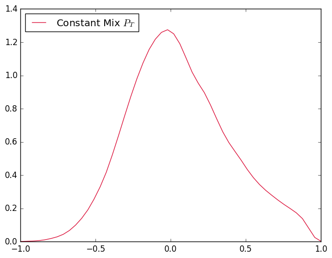
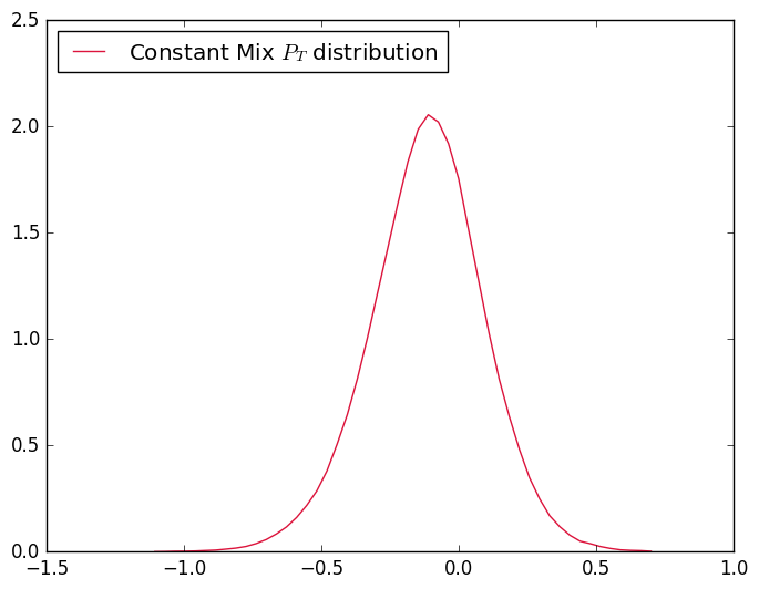
Using the Constant Mix strategy, the normalized $P_{T}$ distribution such that the maximal loss is equal to $-1$ is given on figure 1, so one may wonder how to get a strategy permitting to reduce the risk of high endowments. In the sequel this normalization value will be used for all the distribution quantiles and figures.
We note $\phi=(\phi_{t})$ the proportion of the portfolio $A_{t}$ invested in the equity index at date $t$. The portfolio dynamic is the given by :

$$dA_{t}=\phi_{t}A_{t}((\mu-r)dt+\sigma_{t}dW_{t})+dD_{t}.$$ (3.1)

We propose to use an objective function :

$$J(t,A_{t},D_{t})=\mathop{\rm\mathbb{E}\left(\mathit{g(-P_{T})~{}|~{}{\cal F}_{t}}\right)},$$ (3.2)

where $g$ is function with support on $\mathbb{R}^{+}$ and that we will suppose convex. The optimization problem is then :

$$\hat{J}(t,A_{t},D_{t})=\min_{\phi}\mathop{\rm\mathbb{E}\left(\mathit{g(-P_{T})~{}|~{}{\cal F}_{t}}\right)}.$$ (3.3)

In order to solve (3.3), the deterministic Semi-Lagrangian methods [46] have been successfully used up to a maturity of 10 years. An alternative used for the results presented here consists in discretizing $A_{t}$ and $D_{t}$ on a grid and calculating the expectation involved by Monte Carlo. Using the Stochastic Optimization Library StOpt [47], the calculation was realized on a cluster with MPI parallelization. The grids for the asset discretization used a step of $200$ millions euros, while the endowment level is discretized with a step of $500$ millions Euros. A linear interpolation is used to interpolate a position in the bi-dimensional grid $(A,D)$. The number of simulations used to calculate expectations is chosen equal to $4000$.
The optimization part is followed by a simulation part using the optimal control calculated using $50000$ simulations.

Selection of the objective function to fit risk aversion

On figure 2 we give the normalized distributions obtained by different objective functions $g(x)=g_{1}(x):=(x+0.4x^{2})1_{x>0}$, $g(x)=g_{2}(x):=(x+0.4x^{2}+4e^{-4}x^{3})1_{x>0}$, $g(x)=g_{3}(x):=g(x)=(x+0.4x^{2}+4e^{-5}x^{3})1_{x>0}$ :

$g_{2}(x)=(x+0.4x^{2})1_{x>0}$

$g(x)=(x+0.4x^{2}+4e^{-4}x^{3})1_{x>0}$

$g_{3}(x)=(x+0.4x^{2}+4e^{-5}x^{3})1_{x>0}$

Figure 2: Normalized $P_{T}$ obtained for different objective functions with the Black Scholes model;

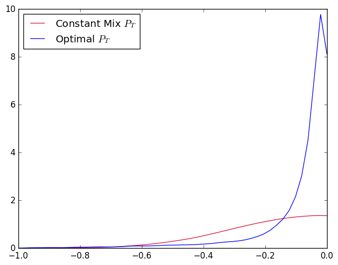
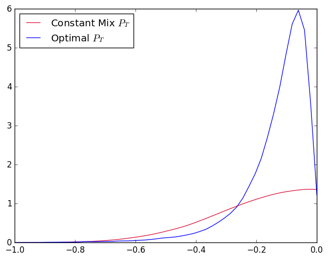
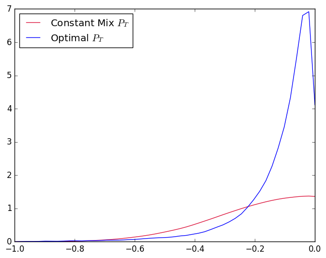
For these three normalized functions we give the different quantiles obtained in table 2.

Quantile	Optimization			Constant Mix
Objective	$g_{1}(x)$	$g_{2}(x)$	$g_{3}(x)$
1%	-0.72380	-0.57396	-0.62012	-0.62889
2%	-0.59356	-0.477630	-0.51152	-0.55947
5%	-0.37616	-0.35093	-0.35795	-0.452577
10%	-0.21702	-0.26972	-0.25986	-0.354676
20%	-0.11440	-0.19472	-0.17181	-0.236149
30%	-0.07264	-0.1533	-0.12504	-0.14848

Table 2: Normalized $P_{T}$ quantile obtained with Black Scholes model with different objective functions.

As expected, it seems to be impossible be get a loss distribution always better than the one obtained Constant Mix. Penalizing the tail as done with function $g_{2}$ permits to get far better results for extreme quantile but degrades the distribution much of the time. With the $g_{1}$ function the optimal distribution is above the Constant Mix in $42\%$ of the case, while with the $g_{2}$ function it is around $30\%$, and with the $g_{3}$ function it is $35\%$. With $g_{2}$ and $g_{3}$, the optimal solution renounces to gains and prefers to secure some quite small losses. In the sequel we restrict ourself to the $g_{3}$ function which seems to fit the practical risk aversion.

Towards an heuristic equivalent to the optimal strategy

Practitioners need to understand the strategy associated to an optimization problem in order to trust it and to check its robustness. We focus for example on the strategy associated to the $g_{3}$ function and we try to explicit the strategy as a function of the funding ratio $\frac{A_{t}-D_{t}}{L_{t}}$ so we approximate $\phi_{t}$ the proportion of the portfolio invested in the equity index by :

$$\phi_{t}\simeq F\left(t,\frac{A_{t}-D_{t}}{L_{t}}\right).$$ (3.4)

On figure 3 we give the strategies at different dates and show that the strategy can be accurately described by a quadratic or cubic fit at each date using some linear regressions.

$\phi_{t}$ with $t=3$ years

$\phi_{t}$ with $t=8$ years

$\phi_{t}$ with $t=15$ years

Figure 3: $\phi_{t}$ simulation for different dates $t$.

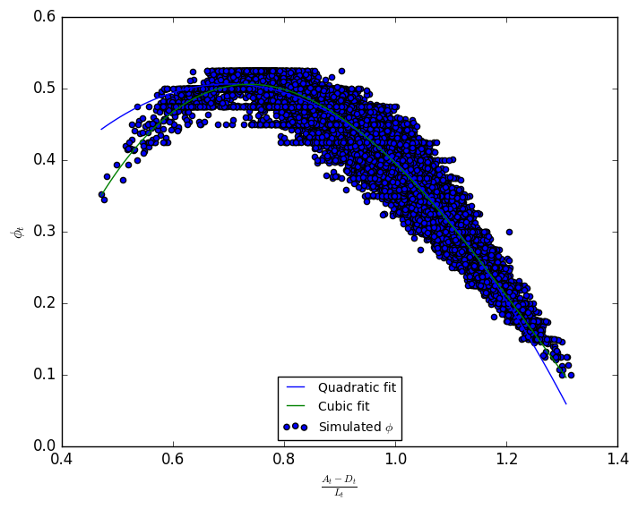
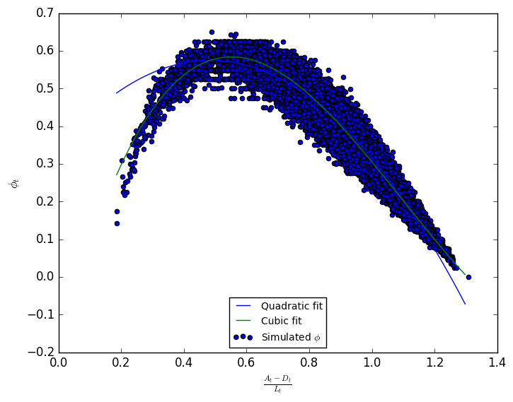
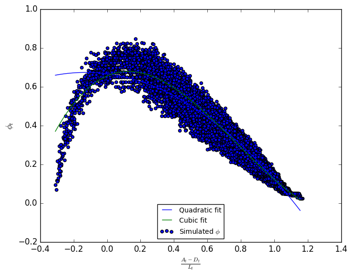
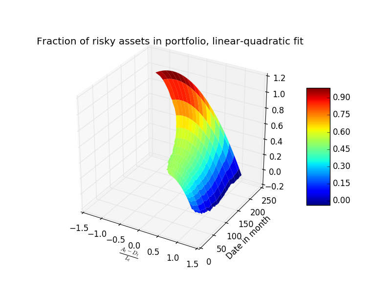
The optimal strategy at each date consists in de-risking the portfolio when the funding ratio is satisfactory and taking more risk when the funding ratio degrades. This optimal strategy can be linked to the de-risking strategies observed with concave strategies. Notice that when the funding ratio becomes very bad and as the time to maturity gets smaller, the strategy consists in de-risking again the portfolio showing that there is no hope to recover the losses. Note that for very high funding ratio the whole portfolio is invested in bonds. According to the preceding results, we look for a linear in time quadratic in space approximation of the strategy :

$$F(t,x)=(a_{0}+a_{1}t)+(b_{0}+b_{1}t)x+(c_{0}+c_{1}t)x^{2}.$$ (3.5)

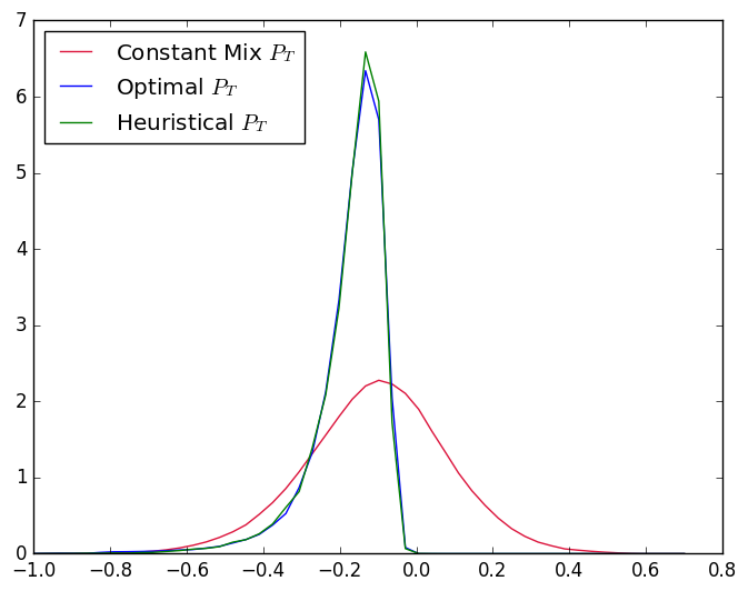
Figure 4 gives the resulting $F$ function and figure 5 shows that the Linear-Quadratic heuristic is very effective.

Figure 4: Linear-Quadratic fit of the strategy, Black Scholes model

Figure 5: Normalized $P_{T}$ distribution with Constant Mix, optimal and Linear-Quadratic heuristic strategy with the Black Scholes model.

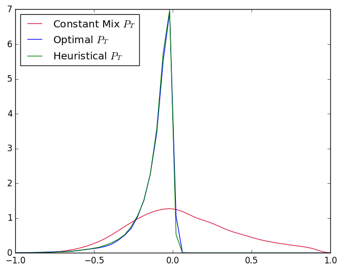
At last we can observe on figure 3 that the optimal strategy is not very dependent on time so we can search for a simple quadratic approximation of the strategy using linear regression. The fitted solution is given by :

$$F(t,x):=F(x)=-0.113x^{2}-0.377x+0.731.$$

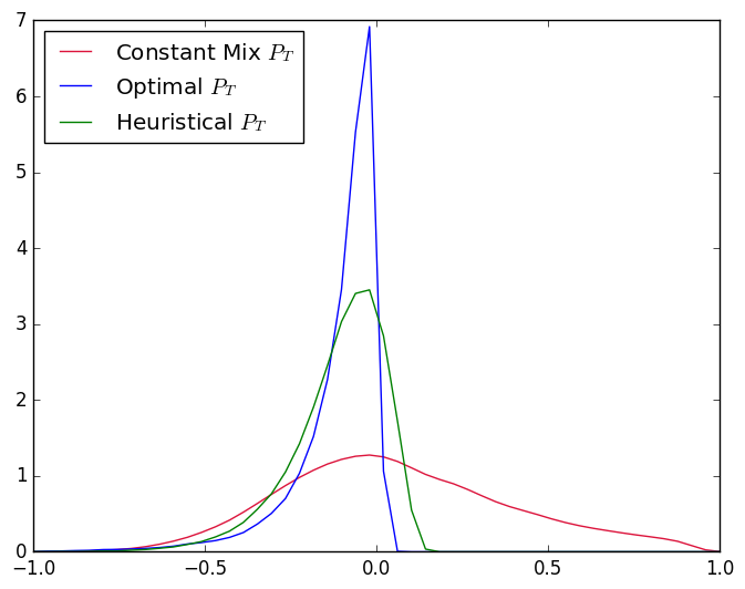
Using this simplified heuristic, we give the $P_{T}$ distribution associated to this strategy on figure 6. The de-risking strategy obtained allows us to gain in the tail as shown on table 3 while not renouncing to some gains : the resulting distribution is more satisfactory from the practitioner point of view (see for example the $1\%$ quantile ) than the “optimal” one indicating that the objective function could be improved.

Figure 6: Comparison of Constant Mix and simplified heuristic normalized $P_{T}$ distribution

Quantile	Simplified	Constant
	heuristic	Mix
1 %	-0.55169	-0.62889
2%	-0.477519	-0.55947
5%	-0.37311	-0.452577
10%	-0.29359	-0.354676
20%	-0.20869	-0.236149
30%	-0.15636	-0.14848

Table 3: Comparison of Constant Mix and simplified heuristic normalized $P_{T}$ quantiles.

Robustness of the strategy

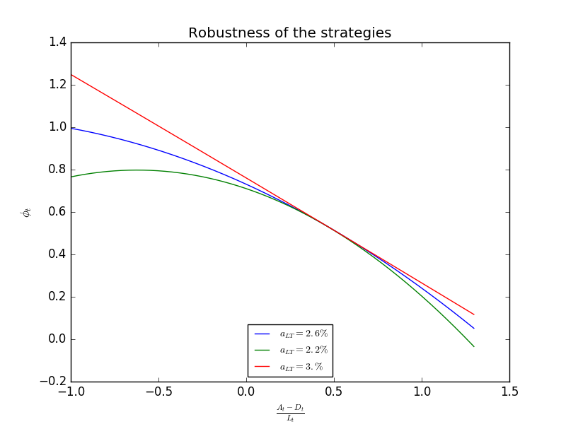
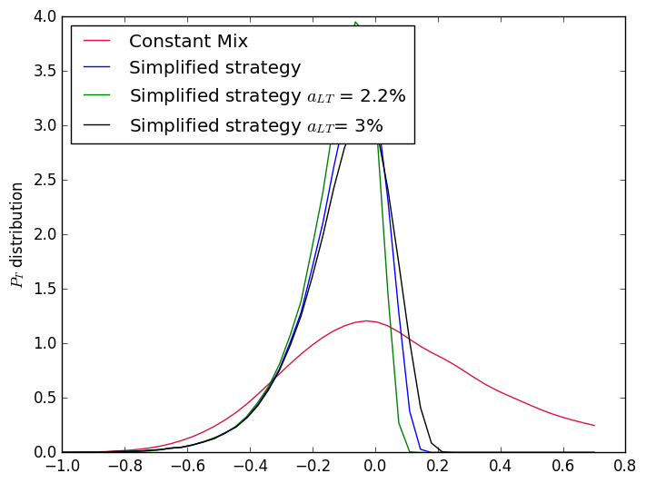
As asserted in the introduction, the principal risk in the short term comes from the long term actualization factor $a_{L}$ that has to be actualized due to the constraint to be below the TEC 30 average value on the last 48 months. We test the robustness of the simplified strategy to a change in the $a_{L}$ value. We still suppose that the ’real’ $a_{L}$ value is equal to $2.6\%$ but that the optimization has been achieved with some different $a_{L}$ values equal to $2.2\%$ or $3\%$. The simplified constant in time quadratic strategy is identified for the two values and reported on figure 7 : as expected the two other strategies are de-risking strategies. On figure 8, we plot the normalized $P_{T}$ distributions using the three simplified heuristics and an $a_{L}$ value equal to $2.6\%$. The figure 8 indicates that the de-risking strategy is stable with respect to the $a_{L}$ parameter.

Figure 7: Testing the sensibility to $a_{L}$ on the strategy.

Figure 8: Testing the sensibility to $a_{L}$ on the $P_{T}$ distribution.

4 Optimal strategy for an index following the MMM model

In this section we take a second modelling for the dynamic of the asset. This modelling is more adapted to long term valorization and will permit to check the robustness of the strategy previously obtained with respect to the model.

The MMM model

This section will allow us to test the strategy robustness with respect to the model used for the equity index.
The Black Scholes model suffers from a lot of shortcomings :

• many studies seem to indicate that the volatility is stochastic with a volatility correlated to the asset [7] explaining the development of models with stochastic volatility [48], [49], [50],

• the observed log returns are not normal giving a skewed distribution with heavy tails explaining the use of jumps and Levy processes to model the prices [51] [52] [53].

But most of all, the long term implicit volatility is far too high yielding for example very high option prices. The success of these models and in particular of the Black Scholes model is due to their Absence Of Arbitrage (AOA) property, equivalent to the existence of martingale measure allowing to give a price to financial assets. As explained in [7], the AOA can be relaxed still giving useful models with arbitrage impossible for strategies keeping positive portfolio values. A similar framework has been developed in [60] and an unified view of these approaches can be found in [61].
In [7], the Minimal Market Model (MMM) has been proposed to model the dynamic of the actualized Growth Optimal Portfolio (GOP). Its dynamic is given by :

$$dS_{t}=\alpha_{t}dt+\sqrt{S_{t}\alpha_{t}}dW_{t},$$ (4.1)

with $\alpha_{t}=\alpha_{0}e^{\eta t},$ where the exponential form permits to model the exponential growth in the economy.
It is showed in [7] that an equi-weighted portfolio with a large number of assets is a good candidate to approximate the GOP. In [7], it is shown for example that the MMM correctly fits the WSI. In the sequel we suppose that our risky index is the MSCI World and that the MMM is a good candidate to modelize the MSCI world actualized dynamic.

$$dS_{t} = \alpha_{t}dt+\sqrt{S_{t}\alpha_{t}}dW_{t}.$$

The advantages of this model are the following:

• it is parsimonious, with only two parameters to fit,

• due to this parsimony, we have a stable and easy way to calibrate the parameters using the empirical covariance of $\sqrt{S_{t}}$ [7],

• the model can be simulated exactly - noting that the equation (4) is a time transformed squared Bessel process of dimension 4 [7] - using the procedure described in [62], [63], [64],

• It keeps the properties of the stochastic volatility models giving high volatilities when the prices is low and low volatilities when the prices are high.

The MMM model has been calibrated on the MSCI World between 1976-2016 yielding the parameters :

$$\alpha_{0} \simeq 2.317$$

$$\eta \simeq 0.0542$$

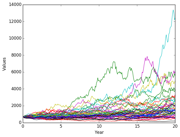
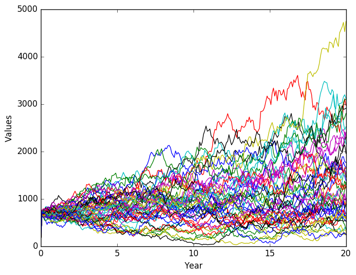
On figure 9 we simulate some prices obtained with the MMM model and the Black Scholes model with $50$ paths showing that the Black Scholes model gives very high values with a high probability.

(a) Some Black Scholes simulations

(b) Some MMM simulations

Figure 9: Some simulations using the Black Scholes and MMM model.

Distribution with Constant Mix Strategy

The distribution obtained by the Constant Mix strategy for the Asset Liability problem is given on table 10.

Figure 10: Normalized $P_{T}$ distribution of the Constant Mix strategy for the MMM (using Black Scholes renormalization factor).

	BS	MMM
Quantile 1%	-0.62889	-0.64045
Quantile 2%	-0.55947	-0.56887
Quantile 3%	-0.51350	-0.52499
Quantile 5%	-0.45257	-0.46535
Quantile 10%	-0.35467	-0.37876
Quantile 20%	-0.23614	-0.28117

Table 4: Normalized $P_{T}$ quantiles of the Constant Mix strategy with the Black Scholes and the MMM (using Black Scholes renormalization factor).

Objective function

Comparing the quantiles obtained in table 4 for the MMM and the Black Scholes model we notice that the quantiles for the losses up to $10\%$ are very close but as expected that the distributions of the gains are very different : due to the volatility structure of the model, a lot of Black Scholes simulations give very unrealistic high returns.
With the MMM dynamic, the portfolio follows the following Stochastic Differential Equation :

$$dA_{t}=\frac{A_{t}}{S_{t}}(\alpha_{t}dt+\sqrt{S_{t}\alpha_{t}}dW_{t})+dD_{t},$$ (4.2)

thus the objective function given by equation (3.2) is a function of $t$,$A_{t}$,$S_{t}$ and $D_{t}$, and the optimization problem becomes :

$$\hat{J}(t,A_{t},S_{t},D_{t})=\min_{\phi}\mathop{\rm\mathbb{E}\left(\mathit{g(-P_{T})~{}|~{}{\cal F}_{t}}\right)}.$$ (4.3)

Numerical results

The numerical resolution of (4.3) compared to (3.3) involves a four dimensional problem much harder to tackle with Monte Carlo methods. The risky asset values $S_{t}$ are discretized with $100$ meshes defined by the partition of the values created with $600000$ samples as explained in [47]. All distributions are calculated by simulating the strategies with $50000$ samples.
We keep using $g_{3}$ for the $g$ function in the objective function (4.3). Once again we fit the optimal strategy as a function of the funding ratio according to (3.4) using a linear in time quadratic in space approximation. The $F$ function obtained is given by figure 11. Using this Linear Quadratic heuristic strategy, the $P_{T}$ distribution is given on figure 12 and is very similar to the one obtained by optimization.

Figure 11: Linear-Quadratic fit of the optimal strategy with the MMM.

Figure 12: $P_{T}$ distribution with Constant Mix, optimal and Linear-Quadratic heuristic strategy with the MMM.

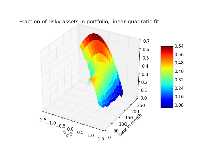
The strategies obtained (optimal and Linear-Quadratic) are very similar to the ones obtained with the Black Scholes model : they are de-risking strategies. They de-risk the portfolio if the funding ratio is good and take some risk if the funding ratio is bad.

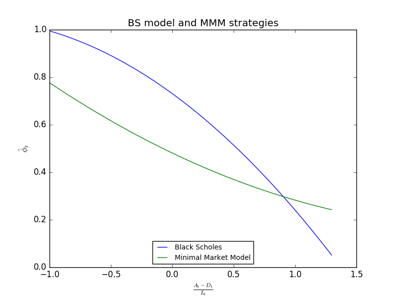
Once again a quadratic independent in time strategy can be computed by regression. A comparison of the de-risking heuristic quadratic strategies obtained by Black Scholes model and the MMM can be found on figure 13. At fist order, the strategies are the same. Once again the quadratic strategy give good results for the tails as shown on table 5.

Figure 13: Comparison of the two Quadratic strategies obtained by the MMM and the Black Scholes model.

Quantile	Constant Mix	Optimized	Linear-Quadratic	Quadratic
			heuristic	heuristic
1%	-0.64045	-0.631190	-0.57322	-0.52199
2%	-0.56887	-0.517330	-0.495545	-0.469857
5%	-0.52499	-0.394088	-0.38883	-0.394860
10%	-0.46535	-0.31676	-0.31524	-0.3374
20%	-0.37876	-0.25002	-0.24987	-0.2779036
30%	-0.28117	-0.21365	-0.21256	-0.23951

Table 5: $P_{T}$ quantiles by optimization, Constant Mix, Linear-Quadratic Heuristic and Quadratic Heuristic in millions of Euros.

At last the figure 14 allows to compare the distribution obtained with the MMM model using the Constant Mix strategy, the one obtained by optimization, the Quadratic strategy calculated, and the Quadratic strategy calculated using a Black Scholes model.

Figure 14: Comparison of distributions obtained on the MMM by the Constant Mix strategy, the optimal strategy, the Quadratic heuristic strategy derived from the MMM optimization and Quadratic strategy calibrated on the Black Scholes model.

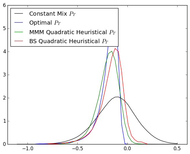
It shows that the result are quite robust with respect to a structural change in the model.

5 Conclusion

We have found that the ALM problem of the French Nuclear Operator can be cast as an optimization problem where the function to optimize penalizes the endowment realized in order to respect the regulatory constraint on the liability. We have shown that the strategy obtained can be easily explained by a de-risking behaviour which is robust with respect to the long term discount factor affecting the liability and that this strategy is also robust to the model choice.

References

- [1] H. M. Markowitz, Portfolio Selection, The Journal of Finance, 7 (1), 77-91, 1952
- [2] R. Michaud, The Markowitz Optimiztion Enigma : Is Optimized Optimal ?, Financial Analysts Journal, Jan-Feb : 149-160, 1995
- [3] V. DeMiguel, L. Garlappin, R. Uppal, Optimal versus naive diversification: How inefficient is the 1/N portfolio strategy?, Management Science 55 (5), 798-812, 2009.
- [4] W. James, C. Stein, Estimation with Quadratic Loss Proceedings of the 4th Berkeley Symposium on Probability and Statistics 1. Berkeley, CA: University of California Press, 1961
- [5] P. Jorion, Bayes-Stein Estimation for Portfolio Analysis, Journal of Financial and Quantitative Analysis, 21:279-292, 1986
- [6] L. Pastor, ´Portfolio Selection and Asset Pricing Models, ˇ Journal of Finance, Vol 55(1) :179-223, 2000
- [7] E. Platen, D. Heath A benchmark Approach to Quantitative Finance, Springer, 2006.
- [8] L. MacLean, E. Thorp, W. Ziemba , The Kelly Capital Growth Investment Criterion, World Scientific Handbook in Financial Economic Series, Vol 3 , 2011
- [9] H. Latané, Criteria for choice among risky ventures, Journal of Political Economy, Vol 38, 145-155, 1959
- [10] L. Breiman, Investment policies for expanding business optimal in a long run sense, Naval Research Logistics Quarterly, Vol7(4), 647-651, 1960
- [11] E. O. Thorp, A favourable strategy for twenty-one. In: Proceedings of the National Academy of Sciences, Vol 47, 110-112, 1961
- [12] H. Markowitz, Investment for the long run: new evidence for an old rule, Journal of Finance XXXI (5), 1273-1286, 1976
- [13] T. Roncalli, Introduction to Risk Parity and Budgeting, Chapman & Hall/CRC Financial Mathematics Series, 2013
- [14] B. Bruder, N. Gaussel, Risk-Return Analysis of Dynamic Investment Strategies, Available at SSRN: http://ssrn.com/abstract=2465623 , 2011
- [15] R. Merton, Optimum Consumption and Portfolio Rules in a Continuous-Time Model, J. Econ. Theory, Vol 45 , 373-413, 1971
- [16] R. Merton, Continuous Time Finance, Blackwell ,1990
- [17] M. Potters, J.P. Bouchaud, Trend followers lose more often than they gain, available at http://arxiv.org/abs/physics/0508104.
- [18] A. Ang, G. Beckaert, International asset allocation with regime shifts, Review of financial studies, Vol 15(4), 1137-1187, 2002
- [19] A. Ang, G. Beckaert, How do regimes affect asset allocation ?, Financial Analysts Journal, Vol 60(2), 86-99, 2004
- [20] M. Guidolin, A. Timmermann, Asset allocation under Multivariate Regime Switching, Journal of Economic Dynamics and Control, Vol 31(11), 3503-3544, 2007
- [21] J. Tu, Is Regime Switching in Stock Returns Important in Portfolio Decisions?, Management Science, Vol 56(7), 1198-1215, 2010
- [22] P. P. Carr, R. A. Jarrow, The Stop-Loss Start-Gain Paradox and Option Valuation: A New Decomposition into Intrinsic and Time Value, Review of Financial Studies, Volume 3(3), 469-492, 1990
- [23] A. F. Perold, Constant Proportion Portfolio Insurrance, manuscript, Harvard Business School, August, 1986
- [24] F. Black, A. F. Perold, Theory of Constant Proportion Portfolio Insurance, Journal of Economic Dynamics and Control, 16(3-4): 403-426.
- [25] F. Black, R. W. Jones, Simplifying Portfolio Insurance, The Journal of Portfolio Management. 14 (1): 48-51, 1987
- [26] F. Black, R. Rouhani, Constant proportion portfolio insurance and the synthetic put option: A comparison, In F. J. Fabozzi (Ed.), Investment Management. Cambridge, Massachusetts: Ballinger, 1989
- [27] R. Cont, P Tankov, Constant Proportion Portfolio Insurance in presence of Jumps in Asset Prices, Mathematical finance, Vol 19(3), 379-401, 2009
- [28] N. Amenc, P. Malaise, L. Martellini, Revisiting core-satellite investing - A dynamic model of relative risk management, Journal of Portfolio Management, vol 31(1), 64-75, 2004
- [29] H. E. Leland, M. Rubinstein, The Evolution of Portfolio Insurance, in D.L. Luskin, ed., Portfolio Insurance: A Guide to Dynamic Hedging, Wiley, 1976
- [30] N. El Karoui, M. Jeanblanc, V. Lacoste, Optimal portfolio management with American capital guarantee, Journal of Control and Dynamic Theory, vol 29, 449-468, 2005
- [31] P. Bertrand, J.-L. Prigent, Portfolio Insurance Strategies: A Comparison of Standard Methods When the Volatility of the Stock Is Stochastic International Journal of Business, Vol 8(4), 461-472, 2003
- [32] P. Bertrand, J.-L. Prigent, Portfolio Insurance Strategies: OBPI versus CPPI, Finance, 26, 5-32, 2005
- [33] R. Zagst, J. Kraus, Stochastic dominance of portfolio insurance strategies OBPI versus CPPI, Annals of Operations Research, Vol 185(1), 75-103, 2011
- [34] L. Martellini, Managing Pension Assets: from Surplus Optimization to Liability-Driven Investment, EDHEC working paper, 2006
- [35] L. Martellini, V. Milhau, Dynamic Allocation Decisions in the Presence of Funding Ratio Constraints, Journal of Pension Economics and Finance, Vol 11, 549-580, (2012)
- [36] S. Sundaresan, F. Zapatero, Valuation, Optimal Asset Allocation and Retirement Incentives of Pension Plans, Review of Financial Studies, Vol 10 , 631-660, 1997
- [37] M. Rudolf, T. Ziemba, Intertemporal Surplus Management, Journal of Economic Dynamics and Control, Vol 28 , 975-990, 2004
- [38] J. Detemple, M. Rindisbacher, Dynamic Asset Liability Management with Tolerance for Limited Shortfalls, Insurance: Mathematics and Economics, Vol 43 , 281-294, 2008
- [39] R. P. Hoevenaars, R. D. Molenaar, P. C. Schotman, T. B. Steenkamp, Strategic Asset Allocation with Liabilities: Beyond Stocks and Bonds, Journal of Economic Dynamics and Control, Vol 32, 2939-2970, 2008
- [40] J. H. Van Binsbergen, M. W. Brandt, Solving Dynamic Portfolio Choice Problems by Recursing on Optimized Portfolio Weights or on the Value Function?, Computational Economics, Vol 29 , 355-367, 2007
- [41] H. Wang, J Yang, Dynamic Asset-Liability Management with Inflation Hedging and Regulatory Constraints, Working paper available at “http://www.efmaefm.org/0EFMAMEETINGS/EFMA
- [42] Cour de Comptes (French public auditor), Les coûts de la filière électronucléaire, Public report, January 2012.
- [43] Y. Jiao, O. Klopfenstein, P. Tankov, Hedging under multiple risk constraints, to appear in Finance and Stochastics.
- [44] F. Black, M. Scholes, The pricing of options and corporate liabilities, J. Political Economy, vol 81, 637-654, 1973
- [45] D.P. Heath, E. Platen, Perfect hedging of index derivatives under a minimal market model, International Journal of Theoretical and Applied Finance, vol 5(7), 757-774, 2002
- [46] X. Warin, Some Non-monotone Schemes for Time Dependent Hamilton-Jacobi-Bellman Equations in Stochastic Control, Journal of Scientific Computing ,Vol 66(3), 1122-1147, 2016
- [47] The StOpt library, https://gitlab.com/stochastic-control/StOpt
- [48] S. L. Heston, A closed-form solution for options with stochastic volatility with applications to bond and currency options, Rev. Finan. Stud., 6(2),327-343, 1993.
- [49] J. Hull, A. White, The pricing of options on assets with stochastic volatilities, J. Finance, 42(2),281-300, 1987.
- [50] E. M. Stein, J. C. Stein, Stock price distributions with stochastic volatility: An analytic approach., Rev. Finan. Stud., 4(4),727-752, 1991.
- [51] S. G. Kou, A jump-diffusion model for option pricing, Management Sci., 48(8),1086-1101, 2002.
- [52] R. C. Merton, Option pricing when underlying stock returns are discontinuous, J. Finan. Econ., 3(1-2),125-144, 1976.
- [53] R. Cont, P. Tankov, Financial Modelling with Jump Processes, Chapman and Hall/CRC Financial Mathematics Series, 2004
- [54] J.B. Long, The numeraire portfolio, J. Financial Economics, 26:29-69, 1990.
- [55] T. Cover Universal portfolios, Math. Finance,1:1-29, 1991
- [56] W. Ziemba, J. Mulvey, Asset and Liability Management Systems for Long-Term Investors , in World Wide Asset and Liability Modeling W. Ziemba and J. Mulvey (eds.), Cambridge University Press, 1998
- [57] S. Brown, The risk and rewards of minimizing shortfall probability, The Journal of Portfolio Management 25(4), 1999
- [58] M. Stutzer A Portfolio Performance Index, Financial Analysts Journal, Volume 56 Issue 3, 2000
- [59] L. MacLean, E. Thorp, W. Ziemba, The Kelly Capital Growth Investment Criterion, World Scientific Handbook in Financial Economic Series, Vol. 3., 2011
- [60] R. Fernholz, I. Karatzas, Stochastic portfolio theory: an overview, . In A. Bensoussan & Q. Zhang (Eds.), Handbook of numerical analysis: Vol. XV. Mathematical Modeling and Numerical Methods in Finance (pp. 89-167). Oxford: North-Holland, 2009
- [61] C. Fontana, W. J. Runggaldier, Diffusion-based models for financial markets without martingale measures Risk Measures and Attitudes, Biagini, F., Richter, A. & Schlesinger, H. (eds.), 45-81, EAA Series, Springer , 2013
- [62] E. Platen, R. Rendek, Simulation of diversified portfolios in a continuous financial market, Zhang, T. & Zhou, X. (eds), Stochastic Analysis and Applications to Finance: Essays in Honour of Jia-an Yan, World Scientific, USA, 385-410,2009
- [63] H. Hulley, E. Platen, Hedging in the long run, Mathematics and Financial Economics, Vol 6, Issue 2, 105-124, 2012
- [64] E. Platen R. Rendek, Exact Scenario Simulation for Selected Multi-dimensional Stochastic Processes, Communications on Stochastic Analysis, Vol 3, No. 3, 443-465, 2009
- [65] J. Baldeaux, K. Ignatieva, E. Platen, A tractable model for indices approximating the growth optimal portfolio, Studies in Nonlinear Dynamics and Econometrics, vol 18, no. 1, pp. 1-21, 2014.