The Power of Normalization: Faster Evasion of Saddle Points

Abstract

A commonly used heuristic in non-convex optimization is Normalized Gradient Descent (NGD) - a variant of gradient descent in which only the direction of the gradient is taken into account and its magnitude ignored. We analyze this heuristic and show that with carefully chosen parameters and noise injection, this method can provably evade saddle points. We establish the convergence of NGD to a local minimum, and demonstrate rates which improve upon the fastest known first order algorithm due to Ge et al. (2015). The effectiveness of our method is demonstrated via an application to the problem of online tensor decomposition; a task for which saddle point evasion is known to result in convergence to global minima.

1 Introduction

Owing to its efficiency, simplicity and intuitive interpretation, Gradient Descent (GD) and its numerous variants are often the method of choice in large-scale optimization tasks, including neural network optimization Bengio (2009), ranking Burges et al. (2005), matrix completion Jain et al. (2010), and reinforcement learning Sutton et al. (1999). Normalized Gradient Descent (NGD) is a less popular alternation of GD, which enjoys the same efficiency and simplicity.

Exploring the limitations of applying GD to non-convex tasks is an important an active line of research. Several phenomena have been found to prevent GD from attaining satisfactory results. Among them are local-minima, and saddle points. Local minima might entrap GD, preventing it from reaching a possibly better solution. Gradients vanish near saddle points, which causes GD to stall. This saddle phenomenon was recently studied in the context of deep learning, where it was established both empirically and theoretically that saddles are prevalent in such tasks, and cause GD to decelerate Saad and Solla (1995); Saxe et al. (2015); Dauphin et al. (2014); Choromanska et al. (2015). Several empirical studies suggest that arriving at local minima is satisfactory for deep learning tasks: in Dauphin et al. (2014), it is asserted that all local minima are of approximately the same quality as the global one. Additionally, in Choromanska et al. (2015) it is argued that global minima may cause overfitting, while local minima are likely to yields sufficient generalization. Very recently, evading saddles was found to be crucial in other non-convex applications, among them are complete dictionary recovery Sun et al. (2015), phase retrieval Sun et al. (2016), and Matrix completion Ge et al. (2016).

This paper studies the minimization of strict-saddle functions $f:\mathbb{R}^{d}\mapsto\mathbb{R}$, which were previously introduced in the pioneering work of Ge et al., Ge et al. (2015). Strict-saddle is a property that captures multi-modality as well as the saddle points phenomenon. Motivated by Choromanska et al. (2015); Dauphin et al. (2014), our goal is to approach at some local minimum of $f$ while evading saddles. We show that Saddle-NGD, a version of NGD which combines noise perturbations, is more appropriate for this task than the noisy-GD algorithm proposed in Ge et al. (2015). In particular, we show that in the offline setting our method requires $\tilde{O}(\eta^{-3/2})$ iterations in order to reach a solution which is $\eta$-approximately (locally) optimal. This improves upon noisy-GD which requires $\tilde{O}(\eta^{-2})$ iterations. Moreover, we show that Saddle-NGD requires $\tilde{O}(d^{3})$ iterations in order to arrive at a basin of some local minimum, while noisy-GD requires $\tilde{O}(d^{4})$ iterations. In the stochastic optimization setting, we can extend our method to achieve the same sample complexity as noisy-GD. Since a single iteration of NGD/GD costs the same, our results imply that NGD ensures an improved running rime over noisy-GD.

Our experimental study demonstrates the benefits of using Saddle-NGD for the setting of online tensor decomposition. The tensor decomposition optimization problem contains both local minima and saddle points with the interesting property that any local minimum is also a global minimum.

1.1 Related Work

Non-convex optimization problems are in general NP-hard and thus most literature on iterative optimization methods focuses on local guarantees. The most natural guarantee to expect GD in this context is to approach a stationary point, namely a point where gradients vanish. This kind of guarantees is provided in Allen-Zhu and Hazan (2016); Ghadimi and Lan (2013), which focus on the stochastic setting. Approaching local minima while evading saddle points is much more intricate than ensuring stationary points. In Dauphin et al. (2014); Sun et al. (2016), it is demonstrated how to avoid saddle points through a trust region approach which utilizes second order derivatives. A perturbed version of GD was explored in Ge et al. (2015), showing both theoretically and empirically that it efficiently evades saddles. Very recently, it was shown in Agarwal et al. (2016) how to use second order methods in order to rapidly approach local minima. Nevertheless, this approach is only practical in settings where Hessian-vector products can be done efficiently.

NGD is well known to guarantee convergence in the offline settings of convex and quasi-convex optimization Nesterov (1984); Kiwiel (2001) . Recently, a stochastic version of NGD was explored in the context of stochastic quasi-convex optimization, Hazan et al. (2015).

2 Setting and Assumptions

We discuss the offline optimization setting, where we aim at minimizing a continuous smooth function $f:\mathbb{R}^{d}\mapsto\mathbb{R}$. The optimization procedure lasts for $T$ rounds, at each round $t\in[T]$ we may query $x_{t}\in\mathbb{R}^{d}$ and receive the gradient, $\nabla f(x_{t})$, as a feedback. After the last round we aim at finding a point $\bar{x}_{T}$ such that $f(\bar{x}_{T})-f(x^{*})$ is small, where $x^{*}$ is some local minimum of $f$.

Strict-Saddle-Property:

We focus on the optimization of strict-saddle functions, a family of multi-modal functions which encompasses objectives that acquire saddle points. Interestingly, Ge et al. (2015) have found that tensor decomposition problems acquire this strict-saddle property.

Definition 1 (Strict-saddle).

Given $\alpha,\gamma,\nu,r>0$ , a function $f$ is $(\alpha,\gamma,\nu,r)$-strict-saddle if for any $x\in\mathbb{R}^{d}$ at least one of the following applies:

1. $\|\nabla f(x)\|\geq\nu$

2. $\lambda_{min}(\nabla^{2}f(x))\leq-\gamma$

3. There exists a local minimum $x^{*}$ such that $\|x-x^{*}\|\leq r$, and the function $f(x)$ restricted to a $2r$ neighbourhood of $x^{*}$ is $\alpha$-strongly-convex.

here $\nabla^{2}f(x)$ denotes the Hessian of $f$ at $x$, and $\lambda_{\min}(\nabla^{2}f(x))$ is the minimal eigenvalue of the Hessian. According to the strict-saddle property, for any $x\in\mathbb{R}^{d}$ at least one of three scenarios applies: either the gradient at $x$ is large, otherwise either we are close to a local minimum or we are in the proximity of a saddle point.

We also assume that $f$ is $\beta$-smooth, meaning:

$$\forall x,y\in\mathbb{R}^{d},\quad\|\nabla f(x)-\nabla f(y)\|\leq\beta\|x-y\|~{}.$$

Lastly, we assume that $f$ has $\rho$-Lipschitz Hessians:

$$\forall x,y\in\mathbb{R}^{d},\quad\|\nabla^{2}f(x)-\nabla^{2}f(y)\|\leq\rho\|x-y\|~{}.$$

here $\|\cdot\|$ denotes the spectral norm when applied to matrices, and the $\ell_{2}$ norm when applied to vectors.

Finally, we recall the definition of strong-convexity:

Definition 2.

A function $f:\mathbb{R}^{d}\mapsto\mathbb{R}$ is called $\alpha$-strongly-convex if for any $x,y\in\mathbb{R}^{d}$ the following applies:

$$f(y)-f(x)\geq\nabla f(x)^{\top}(y-x)+\frac{\alpha}{2}\|x-y\|^{2}~{}.$$

3 Saddle-NGD algorithm and Main Results

In Algorithm 1 we present Saddle-NGD, an algorithm that is adapted to handle strict-saddle functions. The main difference from GD is the use of the direction of the gradients rather than the gradients themselves. Note that most updates are noiseless, yet once every $N_{0}$ rounds we add zero mean gaussian noise $\theta n_{t},\text{where }n_{t}\sim\mathcal{N}(0,I_{d})$, here $I_{d}$ is the $d$-dimensional identity matrix. The noisy updates ensure that once we arrive near a saddle, the direction with most negative eigenvalue will be sufficiently large. This in turn implies a fast evasion of the saddle.

Algorithm 1 Saddle-Normalized Gradient Descent (Saddle-NGD)

  Input: $x_{0}\in\mathbb{R}^{d}$, $T_{\text{tot}}$, learning rate $\eta$

  Set: noise level $\theta=\tilde{\Theta}(\eta)$, noise period $N_{0}=\tilde{\Theta}(\eta^{-1/2})$

  for $t=0\ldots T_{\text{tot}}$  do

     Let $g_{t}:=\nabla f(x_{t})$, and $\hat{g}_{t}=\frac{g_{t}}{\|g_{t}\|}$

     if $(t\;\text{mod}\;N_{0})=0$ then $n_{t}\sim\mathcal{N}(0,\mathcal{I}_{d})$ else $n_{t}=0$ end if

     Update

$$x_{t+1}=x_{t}-\eta\hat{g}_{t}+\theta n_{t}$$

  end for

Following is the main theorem of this paper:

Theorem 3.

Let $\xi\in(0,1)$, $\eta\in(0,{\eta_{\max}})$. Also assume that $f:\mathbb{R}^{d}\mapsto\mathbb{R}$ is $(\alpha,\gamma,\nu,r)$-strict-saddle, $\beta$-smooth, has $\rho$-Lipschitz Hessians, and also $|f(x)|\leq B;\;\forall x\in\mathbb{R}^{d}$. Then w.p.$\geq 1-\xi$, Algorithm 1 reaches a point which is $\tilde{O}(\sqrt{\eta})$-close to some local minimum $x^{*}$ of $f$ within $T_{\text{tot}}=\tilde{O}(\eta^{-3/2})$ optimization steps. Moreover:

$$f(x_{T_{\text{tot}}})-f(x^{*})\leq\tilde{O}(\eta)~{}.$$

The above statement holds for a sufficiently small learning rate $\eta\leq\eta_{\max}$. Our analysis shows that $\eta_{\max}=\tilde{O}(1/d^{2})$. We improve upon noisy-GD proposed in Ge et al. (2015), which requires $\tilde{O}(\eta^{-2})$ iterations to reach a point $\tilde{O}(\eta)$ approximately (locally) optimal, and acquired the same dependence of $\eta_{\max}=\tilde{O}(1/d^{2})$.

Notation: Our $\tilde{O}(\cdot),\tilde{\Omega}(\cdot),\tilde{\Theta}(\cdot)$ notation conveys polynomial dependence on $\eta$ and $d$. It hides polynomial factors in $\alpha,\gamma,\beta,\nu,r,\rho,B,\log(1/\eta),\log(d),\log(1/\xi)$.

In fact, since strict-saddle functions are strongly-convex in a $2r$ radius around local minima, our ultimate goal should be arriving $r$-close to such minima. Then we could use the well known convex optimization machinery to rapidly converge. The following corollary formalizes the number of rounds required to reach $r$-close to some local minimum:

Corollary 4.

Let $\xi\in(0,1)$. Assume $f$ as in Theorem 3, then setting $\eta=\min\{\eta_{\max},\tilde{O}(r^{2})\}$ Algorithm 1 reaches $r$-close to some local minimum of $f$ within $T_{\text{tot}}=\tilde{O}(\eta_{\max}^{-3/2})=\tilde{O}(1/d^{3})$ steps, w.p.$\geq 1-\xi$.

Note that the above improves over noisy-GD which requires $\tilde{O}(d^{4})$ steps in order to reach a point $r$-close to some local minimum of $f$ .

3.1 Stochastic Version of Saddle-NGD

In the Stochastic Optimization setting, an exact gradient for the objective function is unavailable, and we may only access noisy (unbiased) gradient estimates. This setting captures some of the most important tasks in machine learning, and is therefore the subject of an extensive study.

Our Saddle-NGD algorithm for offline optimization of strict-saddle functions could be extended to the stochastic setting. This could be done by using minibatches in order to calculate the gradient, i.e. instead of $g_{t}=\nabla f(x_{t})$ appearing in Algorithm 1, we use:

$$g_{t}:=\frac{1}{b}\sum_{i=1}^{b}\mathcal{G}(x_{t},\zeta_{i})~{},$$

here $\{\mathcal{G}(x_{t},\zeta_{i})\}_{i}$ are independent and unbiased estimates of $\nabla f(x_{t})$. Except for this alternation, the stochastic version of Saddle-NGD is similar to the one presented in Algorithm 1. We have found that in order to ensure convergence in the stochastic case, a minibatch $b=\text{poly}(1/\eta)$ is required. This dependence implies that in the stochastic setting Saddle-NGD obtains no better guarantees than noisy-GD. We therefore omit the proof for the stochastic setting.

Nevertheless, we have found that in practice, the stochastic version of Saddle-NGD demonstrates a superior performance compared to noisy-GD. Even when we employ a moderate minibatch size. This is illustrated in Section 6 where Saddle-NGD is applied to the task of online tensor decomposition.

4 Analysis Overview

Our analysis of Algorithm 1 divides according to the three scenarios defined by the strict-saddle property. Here we present the main statements regarding the guarantees of the algorithm for each scenario, and provide a proof sketch of Theorem 3. For ease of notation we assume that we reach at each scenario at $t=0$.

In case that the gradient is sufficiently large, the following ensures us to improve by value within one step:

Lemma 5.

Suppose that $\|g_{0}\|\geq\beta\sqrt{\eta}$, and we use the Saddle-NGD Algorithm, then:

$$\mathbf{E}[f(x_{1})-f(x_{0})\mid x_{0}]~{}\leq~{}-\beta\eta^{3/2}/2~{}.$$

The next lemma ensures that once we arrive close enough to a local minimum we will remain in its proximity.

Lemma 6.

Suppose that $x_{0}$ is $r$-close to a local minimum, i.e., $\|x_{0}-x^{*}\|\leq r$, and $\|g_{0}\|\leq\beta\sqrt{\eta}\leq\nu$. Then the following holds for any $0\leq t\leq\tilde{O}(\eta^{-3/2})$, w.p.$\geq 1-\xi$:

$$\|x_{t}-x^{*}\|^{2}~{}\leq~{}\max\{\|x_{0}-x^{*}\|^{2},\frac{\beta^{2}}{\alpha^{2}}\eta\}+\tilde{O}(\eta)~{}.$$

The next statement describes the improvement attained by Saddle-NGD near saddle points.

Lemma 7.

Let $\xi\in[0,1]$. Suppose that $\|g_{0}\|\leq\beta\sqrt{\eta}\leq\nu$ and we are near a saddle point, meaning that $\lambda_{min}(\nabla^{2}f(x_{0}))\leq-\gamma$. Then w.p.$\geq 1-\xi$, within $t\leq\tilde{O}(\eta^{-1/2})$ steps, we will have :

$$f(x_{t})~{}\leq~{}f(x_{0})-\tilde{\Omega}(\eta)~{}.$$

Theorem 3 is based on the above three lemmas. The full proof of the Theorem appears in Appendix A. Next we provide a short sketch of the proof.

Proof Sketch of Theorem 3.

Loosely speaking, Lemmas 5, 7 imply that as long as we have not reached close to a local minimum, then our per-round improvement is $\tilde{\Omega}(\eta^{3/2})$ (on average). Since $f$ is bounded, this implies that within $\tilde{O}(\eta^{-3/2})$ rounds we reach at some local minimum, $x^{*}$. Lemma 6 ensures that we will remain in the $\tilde{O}(\sqrt{\eta})$ proximity of this local minimum. Finally, since $f$ is $\beta$-smooth, this $\tilde{O}(\sqrt{\eta})$ proximity implies that we reach a point which is $\tilde{O}(\eta)$ close by value to $f(x^{*})$. ∎

5 Analysis

Here we prove the main statements regrading the three scenarios defined by the strict-saddle property. Section 5.1 analyses the scenario of large gradients (Lemma 5), Section 5.2 analyses the local-minimum scenario (Lemma 6), and Section 5.3 analyses the case of saddle points (Lemma 7). For brevity we do not always provide full proofs, which are deferred to appendix.

5.1 Large Gradients

Proof of Lemma 5.

We will prove assuming a noisy update, i.e. $x_{1}=x_{0}-\eta\hat{g}_{0}+\theta n_{0}$ and $n_{0}\sim\mathcal{N}(0,I_{d})$ (the noiseless update case is similar). By the update rule:

$$\mathbf{E}[f(x_{1})-f(x_{0})\mid x_{0}] ~{}\leq~{}\mathbf{E}[g_{0}^{\top}(x_{1}-x_{0})+\frac{\beta}{2}\|x_{1}-x_{0}\|^{2}\mid x_{0}]$$

$$~{}=~{}\mathbf{E}[g_{0}^{\top}(-\eta\hat{g}_{0}+\theta n_{0})+\frac{\beta}{2}\|-\eta\hat{g}_{0}+\theta n_{0}\|^{2}\mid x_{0}]$$

$$~{}=~{}-\eta\|g_{0}\|+\frac{\beta}{2}(\eta^{2}+d\theta^{2})$$

$$~{}\leq~{}-\beta\eta^{3/2}+\frac{\beta}{2}(\eta^{2}+d\theta^{2})$$

$$~{}\leq~{}-\beta\eta^{3/2}/2$$

here we used $\mathbf{E}[n_{0}]=0$, $\mathbf{E}\|n_{0}\|^{2}=d$, the smoothness of $f$, $\|\hat{g}_{0}\|=1$, and the last inequality uses $d\theta^{2}=d\tilde{\Theta}(\eta^{2})<\eta^{3/2}/4$, which holds if we choose $\eta=\tilde{O}(1/d^{2})$. In order for the other scenarios to hold when the gradient is small we require $\beta\sqrt{\eta}\leq\nu$. ∎

5.2 Local Minimum

For brevity we will not prove Lemma 6, but rather state and prove a simpler lemma assuming all updates are noiseless; the proof of Lemma 6 regarding the general case appears in Appendix B.

Lemma 8.

Suppose that $x_{0}$ is close to a local minimum $x^{*}$, i.e., $\|x_{0}-x^{*}\|\leq r$, and $\|g_{0}\|\leq\beta\sqrt{\eta}\leq\nu$. Then the following holds for any $t\geq 0$:

$$\|x_{t}-x^{*}\|^{2}~{}\leq~{}\max\{\|x_{0}-x^{*}\|^{2},\frac{2\beta^{2}}{\alpha^{2}}\eta^{2}\}~{}.$$

Proof.

Due to the local strong-strong convexity of $f$ around $x^{*}$, we know that $\|x_{0}-x^{*}\|\leq\frac{1}{\alpha}\|g_{0}\|\leq\frac{\beta}{\alpha}\sqrt{\eta}$. In order to be consistent with the definition of strict-saddle property we choose $\eta$ such that $\frac{\beta}{\alpha}\sqrt{\eta}\leq r$.

The proof requires the following lemma regarding strongly-convex functions:

Lemma 9.

Let $F:\mathbb{R}^{d}\mapsto\mathbb{R}$ be an $\alpha$-strongly convex function, let $x^{*}=\operatorname*{arg\,min}_{x\in\mathbb{R}^{d}}F(x)$ then the following holds for any $x\in\mathbb{R}^{d}$:

$$\nabla F(x)^{\top}(x-x^{*})\geq\alpha\|x-x^{*}\|^{2}~{}.$$

We are now ready to prove Lemma 8 by induction, assuming all updates are noiseless, i.e. $x_{t+1}=x_{t}-\eta\hat{g}_{t}$. Note that the case $t=0$ naturally holds, next we discuss the case where $t\geq 1$. First assume that $\|x_{t}-x^{*}\|\geq\frac{\beta}{\alpha}\eta$, the noiseless Saddle-NGD update rule implies:

$$\|x_{t+1}-x^{*}\|^{2} ~{}=~{}\|x_{t}-x^{*}\|^{2}-2\eta\hat{g}_{t}^{\top}(x_{t}-x^{*})+\eta^{2}$$

$$~{}=~{}\|x_{t}-x^{*}\|^{2}-2\eta\frac{1}{\|g_{t}\|}{g}_{t}^{\top}(x_{t}-x^{*})+\eta^{2}$$

$$~{}\leq~{}\|x_{t}-x^{*}\|^{2}-2\eta\frac{1}{\|g_{t}\|}\alpha\|x_{t}-x^{*}\|^{2}+\eta^{2}$$

$$~{}\leq~{}\|x_{t}-x^{*}\|^{2}-2\eta\frac{\alpha}{\beta}\|x_{t}-x^{*}\|+\eta^{2}$$

$$~{}\leq~{}\|x_{t}-x^{*}\|^{2}$$

$$~{}\leq~{}\max\{\|x_{0}-x^{*}\|^{2},\frac{2\beta^{2}}{\alpha^{2}}\eta^{2}\}~{},$$

here the first inequality uses Lemma 9, the second inequality uses $\|g_{t}\|\leq\beta\|x_{t}-x^{*}\|$ which follows from smoothness, and the third inequality uses $\|x_{t}-x^{*}\|\geq\frac{\beta}{\alpha}\eta$.

For the case where $\|x_{t}-x^{*}\|\leq\frac{\beta}{\alpha}\eta$ similarly to the above we can conclude that:

$$\| x_{t}-x^{*}\|^{2}$$

$$~{}=~{}\|x_{t}-x^{*}\|^{2}-2\eta\hat{g}_{t}^{\top}(x_{t}-x^{*})+\eta^{2}$$

$$~{}\leq~{}\|x_{t}-x^{*}\|^{2}+\eta^{2}$$

$$~{}\leq~{}\frac{2\beta^{2}}{\alpha^{2}}\eta^{2}$$

$$~{}\leq~{}\max\{\|x_{0}-x^{*}\|^{2},\frac{2\beta^{2}}{\alpha^{2}}\eta^{2}\}~{},$$

we use $\hat{g}_{t}^{\top}(x_{t}-x^{*})\geq 0$, which follows by the local strong-convexity around $x^{*}$. ∎

5.3 Saddle Points

Intuition and Proof Sketch

We first provide some intuition regarding the benefits of using NGD rather than GD in escaping saddles. Later we present a short proof sketch of Lemma  7.

Intuition: NGD vs. GD for a Pure Saddle

Lemma 7 states the decrease in function values attained by the Saddle-NGD near saddle points. Intuitively, Saddle-NGD implicitly performs an approximate power method over the Hessian matrix $H_{0}:=\nabla^{2}f(x_{0})$. Since the gradients near saddle points tend to be small the use of normalized gradients rather than the gradients themselves yields a faster improvement.
Consider the minimization of a pure saddle function: $F(x_{1},x_{2})=x_{1}^{2}-x_{2}^{2}$. As can be seen in Figure 1, the gradients are almost vanishing around the saddle point $(0,0)$. Conversely, the normalized gradients (Figure 1) are of a constant magnitude. This intuitively suggets that using NGD instead of (noisy) GD yields a faster escape of the saddle. Figure 1 compares between NGD and (noisy) GD for the pure saddle function; both methods are initialized in the proximity of $(0,0)$, and employ a learning rate of $\eta=0.01$. As expected, NGD attains a much faster initial improvement. Later, when the gradients are sufficiently large, GD prevails. Since our goal is the optimization of a general family of functions where saddles behave like pure saddles only locally, we are mostly concerned about the initial local improvement in the case of a pure saddles. This renders NGD more appropriate than GD for our goal.

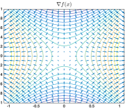
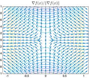
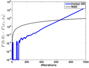
Figure 1: GD vs. NGD around a pure saddle. Left: gradients. Middle: normalized gradients. On the Right we compare GD against NGD, we present $F(0,0)-F(x_{1},x_{2})$ vs. $\#$iterations.

Proof sketch of Lemma  7.

Let $x_{0}$ be a point such that $\|\nabla f(x_{0})\|\leq\beta\sqrt{\eta}$, and also let $\lambda_{\min}(\nabla^{2}f(x_{0}))\leq-\gamma$. Letting $H_{0}=\nabla^{2}f(x_{0})$, it can be shown that the Saddle-NGD update rule implies:

$$\nabla f(x_{t})~{}=~{}\!\left(I-\frac{\eta H_{0}}{\|\nabla f(x_{t-1})\|}\right)\!\nabla f(x_{t-1})+\mu_{t}-\theta H_{0}n_{t}~{},$$ (1)

where $\mu_{t}\leq\tilde{O}(\eta^{3/2})$ for any $t\leq\tilde{O}(\eta^{-1/2})$. Note that the above suggests that Saddle-NGD implicitly performs an approximate power method over the gradients of $f$, with respect to the matrix $A_{t}:=\!\left(I-\frac{\eta H_{0}}{\|\nabla f(x_{t-1})\|}\right)\!$.
There are two differences compared to the traditional power method: first, the multiplying matrix changes from one round to another depending on $\|\nabla f(x_{t-1})\|$, which is a consequence of the normalization. Second, there is an additional additive term $\mu_{t}$, which is related to the deviation of the objective (and its gradients) from its second order taylor approximation around $x_{0}$.

When the gradients are small, the dependence on $\|\nabla f(x_{t-1})\|$ amplifies the increase (resp. decrease) in the magnitude of the components related the negative (resp. positive) eigenvalues of $H_{0}$. Concretely, it can be shown that whenever $\|\nabla f(x_{t-1})\|\leq O(\sqrt{\eta})$, then the gradient component which is related to the eigenvector with the most negative eigenvalue of $H_{0}$, blows up by a factor of $1+O(\sqrt{\eta})$ at every round (ignoring $\mu_{t}$ and the noise term for now). This blow up factor means that within $\tilde{O}(\eta^{-1/2})$ rounds this component increases beyond some threshold value ($\geq 2\beta\sqrt{\eta}$).

Intuitively, the increase in the magnitude of components related to the negative eigenvalues decreases the objective’s value. The proof goes on by showing that the components of gradients/query-points related to the positive eigenvectors of $H_{0}$, do not increase by much. This in turn allows to show that the objective’s value decreases by $\tilde{\Omega}(\eta)$ within $\tilde{O}(\eta^{-1/2})$ iterations.

The noise injections utilized by Saddle-NGD ensure that the additive term, $\mu_{t}$, does not interfere with the increase of the components related to the negative eigenvectors. Since $\mu_{t}$ is bounded, a careful choice of the noise magnitude ensures that there is a sufficiently large initial component in these directions. ∎

Analysis

Before proving Lemma 7 we introduce some notation and establish several lemmas regarding the dynamics of the Saddle-NGD update rule near a saddle point.

Quadratic approximation:

Let $x_{0}$ be a point such that $\nabla f(x_{0})\leq\beta\sqrt{\eta}$, and also $\lambda_{\min}(\nabla^{2}f(x_{0}))\leq-\gamma$ (w.l.o.g. we assume $\lambda_{min}(\nabla^{2}f(x_{0}))=-\gamma$). Denote by $\tilde{f}(x)$ the quadratic approximation of $f$ around $x_{0}$, i.e.:

$$\tilde{f}(x)~{}=~{}f(x_{0})+g_{0}^{\top}(x-x_{0})+\frac{1}{2}(x-x_{0})^{\top}H_{0}(x-x_{0})~{}.$$ (2)

here $g_{0}=\nabla f(x_{0})$, $H_{0}=\nabla^{2}f(x_{0})$. For simplicity we assume that $H_{0}$ is full rank . This implies that there exist $\bar{x}_{0},C$, such that: $\tilde{f}(x)=C+\frac{1}{2}(x-\bar{x}_{0})^{\top}H_{0}(x-\bar{x}_{0})$. Without loss of generality we assume $\bar{x}_{0}=0,C=0$. Thus the quadratic approximation is of the following form:

$$\tilde{f}(x)~{}=~{}\frac{1}{2}x^{\top}H_{0}x~{}.$$ (3)

Along this section, we will interchangeably use Equations (2) and (3) for $\tilde{f}$.

Let $\{e_{i}\}_{i=1}^{d}$ be an orthonormal eigen-basis of $H_{0}$ with eigenvalues $\{\lambda_{i}\}_{i=1}^{d}$:

$$H_{0}~{}=~{}\sum_{i}\lambda_{i}e_{i}e_{i}^{\top}~{}.$$

Also assume without loss of generality that $e_{1}$ is the direction with the most negative eigenvector, i.e. $\lambda_{1}=-\gamma$. We represent each point in the eigen-basis of $H_{0}$, i.e.,

$$x_{t}~{}=~{}\sum_{i}\alpha_{t}^{(i)}e_{i}~{},$$

and therefore

$$\nabla\tilde{f}(x_{t})~{}=~{}H_{0}x_{t}~{}=~{}\sum_{i}\lambda_{i}\alpha_{t}^{(i)}e_{i}~{}.$$

Denoting $g_{t}^{(i)}=e_{i}^{\top}g_{t},\;n_{t}^{(i)}=e_{i}^{\top}n_{t}$; the NGD update rule: $x_{t+1}=x_{t}-\eta\frac{g_{t}}{\|g_{t}\|}+\theta n_{t}$, translates coordinate-wise as follows:

$$\alpha_{t+1}^{(i)}~{}=~{}\alpha_{t}^{(i)}-\eta\frac{g_{t}^{(i)}}{\|g_{t}\|}+\theta n_{t}^{(i)}~{}.$$

Part 0:

Here we bound the difference between the gradients of the original function $f$ and the gradients of the quadratic approximation $\tilde{f}$, and show that these are bounded by the square norm of the distance between $x$ and $x_{0}$. This bound will be useful during the proofs since we decompose the the $x_{t}$’s and their gradients according to the Hessian at $x_{0}$.

For any $x\in\mathbb{R}^{d}$, the gradient, $\nabla f(x)$, can be expressed as follows:

$$\nabla f(x)~{}=~{}\nabla f(x_{0})+\int_{s=0}^{1}H(x_{0}+s(x-x_{0}))ds(x-x_{0})~{}.$$

The above enables to relate the gradient of the original function to the gradient of the approximation:

$$\| \nabla f(x)-\nabla\tilde{f}(x)\|$$

$$~{}=~{}\|\nabla f(x)-\left(\nabla f(x_{0})+H(x_{0})(x-x_{0})\right)\|$$

$$~{}=~{}\left\|\int_{s=0}^{1}\left[H(x_{0}+s(x-x_{0}))-H(x_{0})\right]ds(x-x_{0})\right\|$$

$$~{}\leq~{}\int_{s=0}^{1}\rho sds\|x-x_{0}\|^{2}$$

$$~{}=~{}\frac{\rho}{2}\|x-x_{0}\|^{2}~{},$$ (4)

the above uses the $\rho$-Lipschitzness of the Hessian.

Part 1:

Here we show that the value of the objective does not rise by more than $\tilde{O}(\eta^{3/2})$ in the first $\tilde{O}(\eta^{-1/2})$ rounds. First note the following two lemmas showing that the magnitude of $x_{t}$’s components in directions with positive (resp. negative) eigenvalues do not increase (resp. decrease) by much.

Lemma 10.

Let $T=\tilde{O}(\eta^{-1/2})$. If $\lambda_{i}\geq 0$ then for any $t\in[T]$:

$$|\alpha_{t}^{(i)}|~{}\leq~{} \max\{\eta,|\alpha_{0}^{(i)}|\}+\tilde{O}(\eta)$$

$$+ \begin{cases}\eta&\quad\text{if $\lambda_{i}|\alpha_{0}^{(i)}|\geq\frac{\rho(\eta T)^{2}}{2}$ }\\ \eta\min\{1+\frac{\rho\eta T^{2}}{2\lambda_{i}},T\}&\quad\text{otherwise }\end{cases}$$

Lemma 11.

Let $T\leq\tilde{O}(\eta^{-1/2})$. If $\lambda_{i}\leq 0$ then there exist $c\in[0,1]$ such that $\forall t\in[T]$:

$$|\alpha_{t}^{(i)}|~{}\geq~{}\begin{cases}|\alpha_{0}^{(i)}-\tilde{O}(\eta)|&\quad\text{if $\lambda_{i}|\alpha_{0}^{(i)}|>\frac{\rho(\eta T)^{2}}{2}$ }\\ \left||\alpha_{0}^{(i)}|-c\eta T-\tilde{O}(\eta)\right|&\quad\text{otherwise }\end{cases}$$

The following two corollaries of Lemmas 10, 11 show that the objective’s value does not rise beyond $\tilde{O}(\eta^{3/2})$ within $\tilde{O}(\eta^{-1/2})$ rounds.

Corollary 12.

Let $2\leq T=\tilde{O}(\eta^{-1/2})$, and assume that $\|g_{0}\|\leq\beta\sqrt{\eta}$. Then if $\lambda_{i}>0$ and we start in a saddle, the following holds for all $t\in[T]$:

$$\lambda_{i}\left((\alpha_{t}^{(i)})^{2}-(\alpha_{0}^{(i)})^{2}\right)~{}\leq~{}\tilde{O}(\eta^{3/2})~{}.$$

Corollary 13.

Let $1\leq T\leq\tilde{O}(\eta^{-1/2})$. Then if $\lambda_{i}\leq 0$ and we start in a saddle, the following holds for all $t\in[T]$:

$$|\lambda_{i}|\left((\alpha_{t}^{(i)})^{2}-(\alpha_{0}^{(i)})^{2}\right)~{}\geq~{}-\tilde{O}(\eta^{3/2})~{}.$$

Part 2:

Here we show that the objective’s value decreases by $\tilde{\Omega}(\eta)$ within the first $\tilde{O}(\eta^{-1/2})$ rounds. First note the next lemma showing that the norm of the gradient rises beyond $2\beta\sqrt{\eta}$ within $\tilde{O}(\eta^{-1/2})$ rounds.

Lemma 14.

With a probability$\geq 1-\xi$, the norm of the gradients rises beyond $2\beta\sqrt{\eta}$ within less than $\tilde{O}(\eta^{-1/2})$ steps.

Next we show that whenever $\|g_{t}\|\geq 2\beta\sqrt{\eta}$ then we have improved by value.

Lemma 15.

Suppose we are in a saddle, and $\|g_{0}\|\leq\beta\sqrt{\eta}$ then for the first $t$ such that $\|g_{t}\|\geq 2\beta\sqrt{\eta}$, the following holds w.p.$\geq 1-\xi$

$$f(x_{t})~{}\leq~{}f(x_{0})-\Omega(\eta)~{}.$$

We are now ready to prove Lemma 7

Proof of Lemma 7.

The Lemma follows directly by Lemmas 14, 15. ∎

In Appendix C we provide the complete proofs for the statements that appear in this section.

6 Experiments

In many challenging machine learning tasks, first and second order moments are not sufficient in order to extract the underlying parameters of the problem; and higher order moments are required. Such problems include Gaussian Mixture Models (GMMs), Independent Component Analysis (ICA), Latent Dirichlet Allocation (LDA), and more. Tensors of order greater than $2$ may capture such high order statistics, and their decomposition enables to reveal the underlying parameters of the problem (see Anandkumar et al. (2014) with references therein). Thus, tensor decomposition methods have been extensively studied over the years Harshman (1970); Kolda (2001); Anandkumar et al. (2014). While most studies of tensor decomposition methods have focused on the offline setting, Ge et al. (2015) recently proposed a new setting of online tensor decomposition which is more appropriate for big data tasks.

Tensor decomposition is an intriguing multi-modal optimization task, which provably acquires many saddle points. Interestingly, every local minimum is also a global minimum for this task. Thus we decided to focus our experimental study on this task.

In what follows, we briefly review tensors and the online decompositions task. Then we present our experimental results comparing our method to noisy GD, which was proposed in Ge et al. (2015).

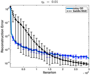
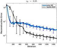
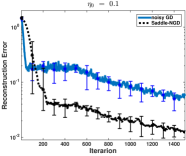
Figure 2: Noisy-GD Vs. Saddle-NGD for the online ICA problem.

Tensor Decomposition

A $p$-th order tensor $T\in\bigotimes^{p}\mathbb{R}^{d}$ is a $p$ dimension array. Here we focus on $4$-th order tensors $T\in\bigotimes^{4}\mathbb{R}^{d}$, and use $T_{i_{1},i_{2},i_{3},i_{4}},\;(i_{1},i_{2},i_{3},i_{4}\in[d])$ to denote the $(i_{1},i_{2},i_{3},i_{4})$-th entry of $T$. For a vector $v\in\mathbb{R}^{d}$ we use $v^{\otimes 4}$ to denote its $4$-th tensor power:

$$(v^{\otimes 4})_{i_{1},i_{2},i_{3},i_{4}}~{}=~{}v_{i_{1}}v_{i_{2}}v_{i_{3}}v_{i_{4}}~{}.$$

We may represent $T\in\bigotimes^{4}\mathbb{R}^{d}$ as a multilinear map, such that $\forall u,v,z,w\in\mathbb{R}^{d}$:

$$T(u,v,z,w)~{}=~{}\sum_{i_{1},i_{2},i_{3},i_{4}}T_{i_{1},i_{2},i_{3},i_{4}}u_{i_{1}}v_{i_{2}}z_{i_{3}}w_{i_{4}}~{}.$$

We say that $T\in\bigotimes^{4}\mathbb{R}^{d}$ has an orthogonal decomposition, if there exists an orthonormal basis $\{a_{i}\in\mathbb{R}^{d}\}_{i=1}^{d}$ such that:

$$T~{}=~{}\sum_{i=1}^{d}a_{i}^{\otimes 4}~{}.$$

and we call $\{a_{i}\}_{i=1}^{d}$ the components of $T$. Given $T$ that has an orthogonal decomposition, the offline decomposition problem is to find its components (which are unique up to permutations and sign flips).

Ge et al. (2015) suggest to calculate the components of a decomposable tensor $T$ by minimizing the following strict-saddle objective:

$$\min_{\forall i,\|u_{i}\|=1}~{}\sum_{j\neq i}T(u_{i},u_{i},u_{j},u_{j})~{}.$$ (5)

Online Tensor Decomposition:

In many machine learning tasks, data often arrives sequentially (sampled from some unknown distribution). When the dimensionality of the problem is large, it is desirable to store only small batches of the data. In many such tasks where tensor decomposition is required, data samples $\{z_{i}\}_{i}$ arrive from some unknown distribution $\mathcal{D}$. And we aim at decomposing a tensor $T$, which is often an expectation over mulitilinear operators $q(z)$, i.e. $T=\mathbf{E}_{z\sim\mathcal{D}}[q(z)]$. Using the linearity of multilinear maps, and the objective appearing in Equation (5), we can formulate such problems as follows:

$$\min_{\forall i,\|u_{i}\|=1}\mathbf{E}_{z\sim\mathcal{D}}[\phi_{z}(u)]~{},$$ (6)

where $\phi_{z}(u)~{}=~{}\sum_{i\neq j}q(z)(u_{i},u_{i},u_{j},u_{j})$.

ICA task: We discuss a version of the ICA task where we receive samples $y_{i}:=Ax_{i}\in\mathbb{R}^{d}$, $A\in\mathbb{R}^{d\times d}$ is an unknown orthonormal linear transformation and $\{x_{i}\sim\text{Uni}\{{\pm 1}^{d}\}\}_{i}$. Based on the samples $\{y_{i}\}_{i}$, we aim at reconstructing the matrix $A$ (up to permutation of its columns and sign flips). Ge et al. (2015) have shown that the ICA problem can be formulated as in Equation (6), and demonstrated how to calculate $\nabla\phi_{z}(u)$. This enables to use the samples in order to produce unbiased gradient estimates of the decomposition objective (and requires to store only small data minibatches).

ICA Experiments:

We adopt the online tensor decomposition setting for ICA suggested above, and present experimental results comparing our method to the noisy GD method of Ge et al. (2015). We take $d=10$, and our performance measure is the reconstruction error defined as:

$$\mathcal{E}~{}=~{}\left(\|T-\sum_{i}u_{i}^{\otimes 4}\|_{F}\right)^{2}/\|T\|_{F}^{2}~{}.$$

In our experiments, both methods use a minibatch of size $500$ to calculate gradient estimates. Moreover, both methods employ the following learning rate rule:

$$\eta_{t}~{}=~{}\begin{cases}\eta_{0}&\quad\text{if $t\leq 500$ }\\ \frac{500}{t}\eta_{0}&\quad\text{otherwise }\end{cases}~{}.$$ (7)

In Figure 2 we present our results, for three values of initial learning rates $\eta_{0}\in\{0.01,0.05,0.1\}$. As can be seen in all three cases, noisy-GD obtains a faster initial improvement. Yet, at some point the error obtained by Saddle-NGD decreases sharply, and eventually Saddle-NGD outperforms noisy-GD. We found that this behaviour persisted when we employed learning rate rules other than (7). Note that for $\eta_{0}\in\{0.05,0.1\}$ Saddle-NGD outperforms noisy-GD within $\approx 400$ iterations, for $\eta=0.01$ this only occurs after $\approx 2\cdot 10^{4}$ iterations.

7 Discussion

We have demonstrated both empirically and theoretically the benefits of using normalized gradients rather than gradients for an intriguing family of non-convex objectives. It is natural to ask what are the limits of the achievable rates for evading saddles. Concretely, we ask wether we can do better than Saddle-NGD using only first order information.

Appendix A Proof of Theorem 3

Proof of Theorem 3.

We will now show that starting at any $x_{0}\in\mathbb{R}^{d}$, within $\tilde{O}(\eta^{-3/2})$ rounds then w.p.$\geq 1/2$ we arrive $\tilde{O}(\sqrt{\eta})$ close to a local minimum. Since this is true for any starting point, repeating this for $\Theta(\log(1/\xi))$ epochs implies that within $\tilde{O}(\eta^{-3/2})$ rounds then w.p.$\geq 1-\xi$ we reach a point that is $\tilde{O}(\sqrt{\eta})$ close to a local minimum.

Let us define the following sets with respects to the three scenarios of the strict saddle property:

$$\mathcal{A}_{1}~{}=~{}\{x:\;\|\nabla f(x)\|\geq\beta\sqrt{\eta}\}$$

$$\mathcal{A}_{2}~{}=~{}\{x:\;\|\nabla f(x)\|<\beta\sqrt{\eta}\text{ and }\lambda_{min}(\nabla^{2}f(x))\leq-\gamma\}$$

$$\mathcal{A}_{3}~{}=~{}\mathcal{A}_{1}^{c}\cap A_{2}^{c}$$

By the strict saddle property, choosing $\eta$ small enough ensures that all points in $\mathcal{A}_{3}$ are $\tilde{O}(\sqrt{\eta})$ close to a local minimum. In what follows we show that with a high probability we reach a point in $\mathcal{A}_{3}$ within $\tilde{O}(\eta^{-3/2})$ rounds.

Define the following sequence of stopping times with $\tau_{0}=0$, and

$$\tau_{i+1}~{}=~{}\begin{cases}\tau_{i}+1&\quad x_{\tau_{i}}\in\mathcal{A}_{1}\cup\mathcal{A}_{3}\\ \tau_{i}+T(x_{\tau_{i}})&\quad x_{\tau_{i}}\in\mathcal{A}_{2}\\ \end{cases}$$

Where given $x\in\mathcal{A}_{2}$ then $T(x)$ is defined to be the first time after that Saddle-NGD reaches a point with a value lower by at least $\tilde{\Omega}(\eta)$ than $f(x)$. Define a sequence of filtrations $\{\mathcal{F}_{t}\}_{t}$, as follows, $\mathcal{F}_{t}=\{x_{0},\ldots,x_{t}\}$, and note that according to Lemma 7 and Lemma 5 the following holds:

$$\mathbf{E}[f(x_{\tau_{i+1}})-f(x_{\tau_{i}})\mid x_{\tau_{i}}\in\mathcal{A}_{1},\mathcal{F}_{\tau_{i}}]~{}\leq~{}-\tilde{\Omega}(\eta^{3/2})$$ (8)

$$\mathbf{E}[f(x_{\tau_{i+1}})-f(x_{\tau_{i}})\mid x_{\tau_{i}}\in\mathcal{A}_{2},\mathcal{F}_{\tau_{i}}]~{}\leq~{}-\tilde{\Omega}(\eta)$$ (9)

The second inequality holds by the following Corollary of Lemma 7

Corollary 16.

Suppose that $\|g_{0}\|\leq\beta\sqrt{\eta}\leq\nu$ and we are in a saddle point, meaning that $\lambda_{min}(\nabla^{2}f(x_{0}))\leq-\gamma$. And consider the Saddle-NGD algorithm performed over a strict-saddle function $f$. Then within $t\leq\tilde{O}(\eta^{-1/2})$ steps, we will have :

$$\mathbf{E}[f(x_{t})-f(x_{0})\mid x_{0}\in\mathcal{A}_{2},\mathcal{F}_{0}]~{}\leq~{}-\tilde{\Omega}(\eta)~{}.$$

Note that according to the above corollary we have $T(x)\leq\tilde{O}(\eta^{-1/2}),\;\forall x\in\mathcal{A}_{2}$. Combining Equations (8),(9) the following holds:

$$\mathbf{E}[f(x_{\tau_{i+1}})-f(x_{\tau_{i}})\mid x_{\tau_{i}}\notin\mathcal{A}_{3}]~{}\leq~{}-(\tau_{i+1}-\tau_{i})\tilde{\Omega}(\eta^{3/2})~{}.$$ (10)

Now define a series of events $\{E_{i}\}_{i}$ as follows $E_{i}=\{\exists j\leq i:x_{\tau_{j}}\in\mathcal{A}_{3}\}$. Note that $E_{i-1}\subset E_{i}$ and therefore $P(E_{i-1})\leq P(E_{i})$. Now consider $f(w_{\tau_{i+1}})1_{E_{i}}$

$$\mathbf{E} [f(x_{\tau_{i+1}})1_{E_{i}}-f(x_{\tau_{i}})1_{E_{i-1}}]$$

$$~{}=~{}\mathbf{E}[f(x_{\tau_{i+1}})1_{E_{i-1}}-f(x_{\tau_{i}})1_{E_{i-1}}]+\mathbf{E}[f(x_{\tau_{i+1}})(1_{E_{i}}-1_{E_{i-1}})]$$

$$~{}=~{}\mathbf{E}[f(x_{\tau_{i+1}})-f(x_{\tau_{i}})]+\mathbf{E}[f(x_{\tau_{i+1}})-f(x_{\tau_{i}})\mid E_{i}^{c}]P(E_{i}^{c})+B(P(E_{i})-P(E_{i-1}))$$

$$~{}\leq~{}\mathbf{E}[f(x_{\tau_{i+1}})-f(x_{\tau_{i}})]-(\tau_{i+1}-\tau_{i})\Omega(\eta^{3/2})P(E_{i}^{c})+B(P(E_{i})-P(E_{i-1}))~{}.$$ (11)

Summing the above equation over $i$ we conclude that:

$$\mathbf{E} [f(x_{\tau_{i+1}})1_{E_{i}}]-f(x_{0})$$

$$~{}\leq~{}\mathbf{E}[f(x_{\tau_{i+1}})-f(x_{0})]-\tau_{i+1}\tilde{\Omega}(\eta^{3/2})P(E_{i}^{c})+B~{}.$$

Since $|f(x)|\leq B,\;\forall x$ we conclude that setting $\tau_{i+1}\geq\tilde{\Omega}(\eta^{-3/2})$ then $P(E_{i})\geq 1/2$. Since this is true for any starting point then performing the Saddle-NGD procedure for $\tilde{O}(\eta^{-3/2})$ rounds ensures that we arrive $\tilde{O}(\sqrt{\eta})$ close to a local minimum ($\mathcal{A}_{3}$) at least once. Lemma 6 ensures that once we arrive at a local minimum we remain at its $\tilde{O}(\sqrt{\eta})$ proximity w.p.$\geq 1-\xi$. Finally, since $f$ is $\beta$-smooth, this $\tilde{O}(\sqrt{\eta})$ proximity implies that we reach a point which is $\tilde{O}(\eta)$ close by value to $f(x^{*})$-the value of the local minimum. ∎

Appendix B Proof of Lemma 6 (Local Minimum)

Here we prove Lemma 6 regarding the local minimum for the general case which includes the noisy updates. In Section B.1 we prove Lemma 9 which is used during the proof of Lemmas 6,8.

Proof of Lemma 6.

Recall that according to Algorithm 1, once we had a noisy update, we use noiseless updates for the following $\Omega(\eta^{-1/2})$ rounds. Now, due to the local strong convexity we know that $\|x_{0}-x^{*}\|\leq\frac{1}{\alpha}\|g_{0}\|\leq\frac{\beta}{\alpha}\sqrt{\eta}$. We will now show that if the distance of $x_{1}$ from the local minimum $x^{*}$ increases beyond $\frac{\beta}{\alpha}\sqrt{\eta}$ due to the noisy update at round $t=0$, then this distance will be decreased below $\frac{\beta}{\alpha}\sqrt{\eta}$ in the following $\tilde{\Theta}(\eta^{-1/2})$ rounds of noiseless updates.

Let us first bound the increase in the square distance to $x^{*}$ due to the first noisy update.

$$\|x_{1}-x^{*}\|^{2} ~{}=~{}\|x_{0}-x^{*}\|^{2}-2(\eta\hat{g}_{0}+\theta n_{0})^{\top}(x_{0}-x^{*})+\|\eta\hat{g}_{0}+\theta n_{0}\|^{2}$$

$$~{}\leq~{}\|x_{0}-x^{*}\|^{2}+\tilde{O}(\eta^{3/2}\sqrt{d})+\tilde{O}(\eta^{2}d)$$

$$~{}\leq~{}\|x_{0}-x^{*}\|^{2}+\eta~{}.$$ (12)

Here we used $\hat{g}_{0}(x_{0}-x^{*})\geq 0$ which follows by local strong-convexity around $x^{*}$, we also used $\theta n_{0}\sim\tilde{O}(\eta)\mathcal{N}(0,\mathcal{I}_{d})$, which implies that w.p.$\geq 1-\xi$ we have $\|\theta n_{0}\|\leq\tilde{O}(\eta\sqrt{d}\log(1/\xi))$. We also used $\|x_{0}-x^{*}\|\leq O(\sqrt{\eta})$. The last inequality follows by choosing $\eta\leq\tilde{O}(1/d)$.

Let $t\geq 2$, and suppose $\|x_{t-1}-x^{*}\|\geq\frac{\beta}{\alpha}\sqrt{\eta}$, the Saddle-NGD update rule implies:

$$\|x_{t}-x^{*}\|^{2} ~{}=~{}\|x_{t-1}-x^{*}\|^{2}-2\eta\hat{g}_{t}^{\top}(x_{t-1}-x^{*})+\eta^{2}$$

$$~{}=~{}\|x_{t-1}-x^{*}\|^{2}-2\eta\frac{1}{\|g_{t}\|}{g}_{t}^{\top}(x_{t-1}-x^{*})+\eta^{2}$$

$$~{}\leq~{}\|x_{t-1}-x^{*}\|^{2}-2\eta\frac{1}{\|g_{t}\|}\alpha\|x_{t-1}-x^{*}\|^{2}+\eta^{2}$$ Lemma 9

$$~{}\leq~{}\|x_{t-1}-x^{*}\|^{2}-2\eta\frac{\alpha}{\beta}\|x_{t-1}-x^{*}\|+\eta^{2}$$ smoothness

$$~{}\leq~{}\|x_{t-1}-x^{*}\|^{2}-\eta\sqrt{\eta} \|x_{t-1}-x^{*}\|\geq\frac{\beta}{\alpha}\sqrt{\eta}$$ (13)

here in the first inequality we use Lemma 9, the second inequality uses $\|g_{t}\|\leq\beta\|x_{t}-x^{*}\|$ which follows from smoothness, and the last inequality uses $\|x_{t-1}-x^{*}\|\geq\frac{\beta}{\alpha}\sqrt{\eta}$.

Combining Equations (B),(B) it follows that within the total of $\Theta(\eta^{-1/2})$ rounds of noiseless updates the distance to the local minimum must decrease to $\frac{\beta}{\alpha}\sqrt{\eta}$. The rest of the proof goes along the same lines as the proof of Lemma 8. ∎

B.1 Proof of Lemma 9

Proof.

Writing the strong-convexity inequality for $F$ at both $x,x^{*}$, and using $\nabla F(x^{*})^{\top}(x-x^{*})\geq 0$, which follows by the optimality of $x^{*}$, we have:

$$F(x^{*})-F(x) ~{}\geq~{}\nabla F(x)^{\top}(x^{*}-x)+\frac{\alpha}{2}\|x-x^{*}\|^{2}$$ (14)

$$F(x)-F(x^{*}) ~{}\geq~{}\frac{\alpha}{2}\|x-x^{*}\|^{2}$$ (15)

summing the above equations the lemma follows. ∎

Appendix C Omitted Proofs from Section 5.3 (Saddle Analysis)

C.1 Proof of Lemma 10

Proof.

Since $T=\tilde{O}(\eta^{-1/2})$, and Saddle-NGD perform noisy updates once every $N_{0}=\Theta(\eta^{-1/2})$ rounds, it follows that the total increase in $|\alpha_{t}^{(i)}|$ due to noisy rounds is bounded by $\theta\frac{T}{N_{0}}=\tilde{O}(\eta)$. Thus in the rest of the proof we assume noiseless updates, and show the following to hold:

$$|\alpha_{t}^{(i)}|~{}\leq~{}\max\{\eta,|\alpha_{0}^{(i)}|\}+\begin{cases}\eta&\quad\text{if $\lambda_{i}|\alpha_{0}^{(i)}|\geq(\rho/2)\eta^{2}T^{2}$ }\\ \eta\min\{1+\frac{\rho\eta T^{2}}{2\lambda_{i}},T\}&\quad\text{otherwise }\end{cases}~{}.$$ (16)

According to Equation (5.3) then for every $x_{t}\in\mathbb{R}^{d}$ we have:

$$g_{t}~{}=~{}\nabla f(x_{t})~{}=~{}\nabla\tilde{f}(x_{t})+\Delta_{t}~{}=~{}H_{0}x_{t}+\Delta_{t}~{},$$

here we used $\tilde{f}(x)=0.5x^{\top}H_{0}x$, and the notation $\Delta_{t}:=\nabla f(x_{t})-\nabla\tilde{f}(x_{t})$. Thus, combining Equation (5.3), together with $\|x_{t}-x_{0}\|\leq\eta T,\;\forall t\in[T]$(which follows by the Saddle-NGD update rule), we obtain:

$$\|\Delta_{t}\|~{}\leq~{}(\rho/2)\eta^{2}T^{2},\quad\forall t\in[T]~{}.$$ (17)

Denote $\Delta_{t}^{(i)}=e_{i}^{\top}\Delta_{t}$, then coordinate-wise the NGD rule translates to

$$\alpha_{t+1}^{(i)} ~{}=~{}\alpha_{t}^{(i)}-\eta\frac{g_{t}^{(i)}}{\|g_{t}\|}$$

$$~{}=~{}\alpha_{t}^{(i)}-\eta\frac{\lambda_{i}\alpha_{t}^{(i)}+\Delta_{t}^{(i)}}{\|g_{t}\|}~{}.$$

First part: First we show that the following always applies:

$$|\alpha_{t}^{(i)}|~{}\leq~{}\max\{\eta,|\alpha_{0}^{(i)}|\}+\eta\min\{1+\frac{\rho\eta T^{2}}{2\lambda_{i}},T\}~{}.$$ (18)

We will prove Equation (18) by showing the following to hold for all $t\in[T]$:

$$|\alpha_{t}^{(i)}|~{}\leq~{}\max\{\eta,|\alpha_{0}^{(i)}|\}+\eta\begin{cases}1+\frac{\rho\eta T^{2}}{2\lambda_{i}}&\quad\text{if $1+\frac{\rho\eta T^{2}}{2\lambda_{i}}\leq T$ }\\ t&\quad\text{otherwise }\end{cases}~{}.$$ (19)

We will now prove Equation (19) by induction. The base case $t=0$ clearly holds. Now assume by the induction assumption that it holds for $t\in[T]$, then we divide into two cases:

Case 1: Suppose that $T\leq 1+\frac{\rho\eta T^{2}}{2\lambda_{i}}$. Since $\alpha_{t}^{(i)}$ can not change by more than $\eta$ in each round then the following holds:

$$|\alpha_{t+1}^{(i)}|~{}\leq~{}|\alpha_{t}^{(i)}|+\eta~{}\leq~{}\max\{\eta,|\alpha_{0}^{(i)}|\}+\eta(t+1)~{}.$$

thus the induction hypothesis of Equation (19) holds in this case.

Case 2: Suppose that $T\geq 1+\frac{\rho\eta T^{2}}{2\lambda_{i}}$. In this case our induction hypothesis asserts:

$$|\alpha_{t}^{(i)}|~{}\leq~{}\max\{\eta,|\alpha_{0}^{(i)}|\}+\eta(1+\frac{\rho\eta T^{2}}{2\lambda_{i}})~{}.$$

If $|\alpha_{t}^{(i)}|\geq\max\{\eta,|\alpha_{0}^{(i)}|\}+\frac{\rho\eta^{2}T^{2}}{2\lambda_{i}}$ then using Equation (17), we conclude that:

$$\text{sign}{}(g_{t}^{(i)})~{}=~{}\text{sign}{}(\lambda_{i}\alpha_{t}^{(i)}+\Delta_{t}^{(i)})~{}=~{}\text{sign}{}(\alpha_{t}^{(i)})~{}.$$

The above implies:

$$|\alpha_{t+1}^{(i)}| ~{}=~{}\left|\alpha_{t}^{(i)}-\eta\frac{g_{t}^{(i)}}{\|g_{t}\|}\right|$$

$$~{}=~{}\left||\alpha_{t}^{(i)}|-\eta\frac{|g_{t}^{(i)}|}{\|g_{t}\|}\right| \text{sign}{}(\alpha_{t}^{(i)})=\text{sign}{}(g_{t}^{(i)})$$

$$~{}\leq~{}\max\left\{\eta\frac{|g_{t}^{(i)}|}{\|g_{t}\|},|\alpha_{t}^{(i)}|\right\}$$

$$~{}\leq~{}\max\{\eta,|\alpha^{(i)}_{t}|\} 0\leq\frac{|g_{t}^{(i)}|}{\|g_{t}\|}\leq 1$$

$$~{}\leq~{}\max\{\eta,|\alpha_{0}^{(i)}|\}+\eta(t+1)~{},$$ Induction hypothesis (20)

thus by Equation (C.1), the induction hypothesis holds.

If $|\alpha_{t}^{(i)}|\leq\max\{\eta,|\alpha_{0}^{(i)}|\}+\frac{\rho\eta^{2}T^{2}}{2\lambda_{i}}$, then since each coordinate does not change more than $\eta$ in each iterartion then we have:

$$|\alpha_{t+1}^{(i)}|~{}\leq~{}|\alpha_{t}^{(i)}|+\eta~{}\leq~{}\max\{\eta,|\alpha_{0}^{(i)}|\}+\frac{\rho\eta^{2}T^{2}}{2\lambda_{i}}+\eta~{},$$

and again, the induction hypothesis holds.

Second part: Here we show that whenever $\lambda_{i}|\alpha_{0}^{(i)}|\geq(\rho/2)\eta^{2}T^{2}$ then the following applies:

$$|\alpha_{t}^{(i)}|~{}\leq~{}\max\{\eta,|\alpha_{0}^{(i)}|\}+\eta~{}.$$ (21)

We will now show by induction that Equation (21) holds for any $t\in[T]$. The base case for $t=0$ clearly holds. Now assume by the Induction Hypothesis that $|\alpha_{t}^{(i)}|\leq\max\{\eta,|\alpha_{0}^{(i)}|\}+\eta$. We now divide into two cases:

Case 1: Suppose that $|\alpha_{t}^{(i)}|\leq\max\{\eta,|\alpha_{0}^{(i)}|\}$. Since each coordinate does not change by more than $\eta$ in each round, then:

$$|\alpha_{t+1}^{(i)}|~{}\leq~{}|\alpha_{t}^{(i)}|+\eta~{}\leq~{}\max\{\eta,|\alpha_{0}^{(i)}|\}+\eta~{},$$

thus, the induction hypothesis holds.

Case 2: Suppose that $|\alpha_{t}^{(i)}|\geq\max\{\eta,|\alpha_{0}^{(i)}|\}$. Recall that $t\in[T]$, and $|\Delta_{t}^{(i)}|\leq(\rho/2)\eta^{2}T^{2}$, thus:

$$\lambda_{i}|\alpha_{t}^{(i)}| ~{}\geq~{}\lambda_{i}|\alpha_{0}^{(i)}|$$

$$~{}\geq~{}(\rho/2)\eta^{2}T^{2}$$

$$~{}\geq~{}|\Delta_{t}^{(i)}|~{}.$$

The above implies that:

$$\text{sign}{}(g_{t}^{(i)})~{}=~{}\text{sign}{}(\lambda_{i}\alpha_{t}^{(i)}+\Delta_{t}^{(i)})~{}=~{}\text{sign}{}(\alpha_{t}^{(i)})$$

In this case, a similar analysis to the one appearing in Equation (C.1), shows:

$$|\alpha_{t+1}^{(i)}|~{}\leq~{}\max\{\eta,|\alpha_{t}^{(i)}|\}\leq\max\{\eta,|\alpha_{0}^{(i)}|\}+\eta~{},$$

and the induction hypothesis holds.

Combining Equations (18),(21), establishes the Lemma. ∎

C.2 Proof of Lemma 11

Proof.

Since $T=\tilde{O}(\eta^{-1/2})$, and Saddle-NGD perform noisy updates once every $N_{0}=\Theta(\eta^{-1/2})$ rounds, it follows that the total decrease in $|\alpha_{t}^{(i)}|$ due to noisy rounds is bounded by $\theta\frac{T}{N_{0}}=\tilde{O}(\eta)$. Thus in the rest of the proof we assume noiseless updates, and show the following to hold for some $c\in[0,1]$:

$$|\alpha_{t}^{(i)}|~{}\geq~{}\begin{cases}|\alpha_{0}^{(i)}|&\quad\text{if $\lambda_{i}|\alpha_{0}^{(i)}|>(\rho/2)\eta^{2}T^{2}$ }\\ \left||\alpha_{0}^{(i)}|-c\eta T\right|&\quad\text{otherwise }\end{cases}~{}.$$ (22)

According to Equation (5.3) then for any $x_{t}\in\mathbb{R}^{d}$ we have:

$$g_{t}~{}=~{}\nabla f(x_{t})~{}=~{}\nabla\tilde{f}(x_{t})+\Delta_{t}~{}=~{}H_{0}x_{t}+\Delta_{t}~{},$$

here we used $\tilde{f}(x)=0.5x^{\top}H_{0}x$, and the notation $\Delta_{t}:=\nabla f(x_{t})-\nabla\tilde{f}(x_{t})$. Thus, combining Equation (5.3), together with $\|x_{t}-x_{0}\|\leq\eta T,\;\forall t\in[T]$ (which follows by the Saddle-NGD update rule), we obtain:

$$\|\Delta_{t}\|~{}\leq~{}(\rho/2)\eta^{2}T^{2},\quad\forall t\in[T]$$

Denote $\Delta_{t}^{(i)}=e_{i}^{\top}\Delta_{t}$, then coordinate-wise the NGD rule translates to

$$\alpha_{t+1}^{(i)} ~{}=~{}\alpha_{t}^{(i)}-\eta\frac{g_{t}^{(i)}}{\|g_{t}\|}$$

$$~{}=~{}\alpha_{t}^{(i)}-\eta\frac{\lambda_{i}\alpha_{t}^{(i)}+\Delta_{t}^{(i)}}{\|g_{t}\|}$$

First part: First we show that the following always applies for some $c\in[0,1]$:

$$|\alpha_{t}^{(i)}|~{}\geq~{}\left||\alpha_{0}^{(i)}|-c\eta T\right|~{}.$$ (23)

Equation (23) follows since by the Saddle-NGD update rule the magnitude of the query points can not decrease by more than $\eta T$ over $T$ rounds.

Second part: Here we show that the following applies whenever $\lambda_{i}|\alpha_{0}^{(i)}|>(\rho/2)\eta^{2}T^{2}$:

$$|\alpha_{t}^{(i)}|~{}\geq~{}|\alpha_{0}^{(i)}|~{}.$$ (24)

We will prove Equation (24), by induction. Clearly the base case $t=0$ holds. Now assume that $|\alpha_{t}^{(i)}|\geq|\alpha_{0}^{(i)}|>(\rho/2\lambda_{i})\eta^{2}T^{2}$. Since $g_{t}^{(i)}=\lambda_{i}\alpha_{t}^{(i)}+\Delta_{t}^{(i)}$, and $|\Delta_{t}^{(i)}|\leq(\rho/2)\eta^{2}T^{2}$, then we necessarily have:

$$\text{sign}{}(g_{t}^{(i)})~{}=~{}\text{sign}{}(\lambda_{i}\alpha_{t}^{(i)})~{}=~{}-\text{sign}{}(\alpha_{t}^{(i)})~{},$$

where we used $\lambda_{i}\leq 0$. Hence,

$$|\alpha_{t+1}^{(i)}|~{}=~{}\left|\alpha_{t}-\eta\frac{g_{t}^{(i)}}{\|g_{t}\|}\right|~{}\geq~{}|\alpha_{t}^{(i)}|~{},$$

and the induction hypothesis holds. Combining Equations (23), (24), proves the lemma. ∎

C.3 Proof of Corollary 12

Proof.

We prove the corollary using Lemma 10. Note that for simplicity we ignore the $\tilde{O}(\eta)$ factors appearing in Lemma 10, considering these factors yields similar guarantees. We divide the proof into two cases which depend on the size of $|g_{0}^{(i)}|$. High $|g_{0}^{(i)}|$: Suppose that $|g_{0}^{(i)}|:=\lambda_{i}|\alpha_{0}^{(i)}|\geq(\rho/2)\eta^{2}T^{2}$

$$\lambda_{i} \left((\alpha_{t}^{(i)})^{2}-(\alpha_{0}^{(i)})^{2}\right)$$

$$~{}\leq~{}\lambda_{i}\left((\max\{\eta,\alpha_{0}^{(i)}\}+\tilde{O}(\eta))^{2}-(\alpha_{0}^{(i)})^{2}\right)$$ Lemma 10

$$~{}\leq~{}\lambda_{i}\left(\max\{\eta^{2},(\alpha_{0}^{(i)})^{2}\}-(\alpha_{0}^{(i)})^{2}\right)+2\lambda_{i}|\alpha_{0}^{(i)}|\tilde{O}(\eta)+\lambda_{i}\tilde{O}(\eta^{2})$$

$$~{}\leq~{}2\beta\eta^{2}+\tilde{O}(\eta^{3/2})=\tilde{O}(\eta^{3/2}) \lambda_{i}|\alpha_{0}^{(i)}|\leq\beta\sqrt{\eta}$$ (25)

where the first inequality uses Lemma 10, and the last inequality uses $\lambda_{i}|\alpha_{0}^{(i)}|=|g_{0}^{(i)}|\leq\beta\sqrt{\eta}$, and $\beta=\max_{i}|\lambda_{i}|$.

Low $|g_{0}^{(i)}|$: Suppose that $|g_{0}^{(i)}|:=\lambda_{i}|\alpha_{0}^{(i)}|\leq(\rho/2)\eta^{2}T^{2}$. Denote $B=\min\{1+\frac{\rho\eta T^{2}}{2\lambda_{i}},T\}$, and note that this expression is maximized when $\lambda_{i}=\frac{\rho\eta T^{2}}{2(T-1)}$.

$$\lambda_{i} \left((\alpha_{t}^{(i)})^{2}-(\alpha_{0}^{(i)})^{2}\right)$$

$$~{}\leq~{}\lambda_{i}\left(\max\{\eta^{2},(\alpha_{0}^{(i)})^{2}\}-(\alpha_{0}^{(i)})^{2}\right)+2\tilde{O}(\eta)\max\left\{\lambda_{i}B\eta,\lambda_{i}|\alpha_{0}^{(i)}|B\right\}+\lambda_{i}B^{2}\tilde{O}(\eta^{2})$$

$$~{}\leq~{}\lambda_{i}\eta^{2}+\tilde{O}(\eta)\max\left\{\frac{\rho\eta^{2}T^{3}}{T-1},\frac{\beta\rho\eta^{2}T^{3}}{2}\right\}+\frac{\rho\eta T^{4}}{2(T-1)}\tilde{O}(\eta^{2})$$

$$~{}\leq~{}\beta\eta^{2}+\tilde{O}((\eta T)^{3})$$

$$~{}=~{}\tilde{O}(\eta^{3/2})~{},$$ (26)

here in the second inequality we used $\lambda_{i}B\leq\frac{\rho\eta T^{3}}{2(T-1)}$, we also used $B\leq T$, $|g_{0}^{(i)}|:=\lambda_{i}|\alpha_{0}^{(i)}|\leq(\rho/2)\eta^{2}T^{2}$, and also $\lambda_{i}B^{2}\leq\frac{\rho\eta T^{4}}{2(T-1)}$. The third inequality uses $T\geq 2$, and the last inequality uses $T=\tilde{O}(\eta^{-1/2})$.

Combining Equations (C.3),(C.3), establishes the lemma. ∎

C.4 Proof of Corollary 13

Proof.

For simplicity we are going to use the following bound of Lemma 11 which ignores the $\tilde{O}(\eta)$ factors in the original lemma (these appear due to the noisy updates):

$$|\alpha_{t}^{(i)}|~{}\geq~{}\begin{cases}|\alpha_{0}^{(i)}|&\quad\text{if $\lambda_{i}|\alpha_{0}^{(i)}|>(\rho/2)\eta^{2}T^{2}$ }\\ \left||\alpha_{0}^{(i)}|-c\eta T\right|&\quad\text{otherwise }\end{cases}~{},$$ (27)

which holds for some $c\in[0,1]$. Including the original $\tilde{O}(\eta)$ factors in the calculations yields an additional factor of $-\tilde{O}(\eta^{3/2}+\eta^{2}T)=-\tilde{O}(\eta^{3/2})$ (recall $T=\tilde{O}(\eta^{-1/2})$).

Using Equation (27) we divide into two cases: Case 1: Suppose that $\lambda_{i}|\alpha_{0}^{(i)}|>(\rho/2)\eta^{2}T^{2}$, then by Equation (27) we have $|\alpha_{t}^{(i)}|\geq|\alpha_{0}^{(i)}|$ and therefore

$$|\lambda_{i}|\left((\alpha_{t}^{(i)})^{2}-(\alpha_{0}^{(i)})^{2}\right)~{}\geq~{}0~{}.$$

Case 2: Suppose that $\lambda_{i}|\alpha_{0}^{(i)}|\leq(\rho/2)\eta^{2}T^{2}$, using Equation (27) we get:

$$|\lambda_{i}|\left((\alpha_{t}^{(i)})^{2}-(\alpha_{0}^{(i)})^{2}\right) ~{}\geq~{}|\lambda_{i}|\left((|\alpha_{0}^{(i)}|-c\eta T)^{2}-(\alpha_{0}^{(i)})^{2}\right)$$

$$~{}\geq~{}-2c|\lambda_{i}\alpha_{0}^{(i)}|\eta T+|\lambda_{i}|c^{2}\left(\eta T\right)^{2}$$

$$~{}\geq~{}-2(\rho/2)\eta^{2}T^{2}\eta T$$

$$~{}\geq~{}-\rho(\eta T)^{3}$$

$$~{}\geq~{}-\tilde{O}(\eta^{3/2})~{},$$

here we used $\lambda_{i}|\alpha_{0}^{(i)}|\leq(\rho/2)\eta^{2}T^{2}$, $c\in[0,1]$, and $T=\tilde{O}(\eta^{-1/2})$. ∎

C.5 Proof of Lemma 14

Proof.

Following is the key relation that enables us to prove the lemma:

$$\nabla f(x_{t}) ~{}=~{}\nabla f(x_{t-1})+\int_{0}^{1}H(x_{t-1}+s(x_{t}-x_{t-1}))ds(x_{t}-x_{t-1})$$

$$~{}=~{}\nabla f(x_{t-1})+H_{0}(x_{t}-x_{t-1})+\mu_{t}~{},$$ (28)

where we denote $\mu_{t}=\int_{0}^{1}[H(x_{t-1}+s(x_{t}-x_{t-1}))-H_{0}]ds(x_{t}-x_{t-1})$.

Using the Saddle-NGD update rule inside Equation (C.5) we obtain:

$$\nabla f(x_{t})~{}=~{}\!\left(I-\frac{\eta H_{0}}{\|\nabla f(x_{t-1})\|}\right)\!\nabla f(x_{t-1})+\mu_{t}-\theta H_{0}n_{t}~{}.$$ (29)

Due to the Lipschitzness of the Hessian, and since $\|x_{t}-x_{t-1}\|\leq\eta$, $\|x_{t}-x_{0}\|\leq\eta t$ , the last term is bounded by $O(\eta^{2}t)$:

$$\|\mu_{t}\|~{}\leq~{}\rho\eta^{2}t~{}.$$

Let us look at the gradient component in the most negative direction $e_{1}$:

$$g_{t+1}^{(1)}~{}=~{}g_{t}^{(1)}(1+\gamma\frac{\eta}{\|g_{t}\|})+\mu_{t}^{\top}e_{1}+\gamma\theta n_{t}^{(1)}~{}.$$ (30)

And recall from Algorithm 1 that $n_{t}$ is zero most rounds (non-zero once every $N_{0}=\tilde{O}(\eta^{-1/2})$ rounds); also recall that for simplicity we assume that in $t=0$ the update is noisy.

Next we will show that taking $|g_{1}^{(1)}|,N_{0}$ that fulfill the following two conditions imply that the magnitude of the gradient rises beyond $2\beta\sqrt{\eta}$ within less than $N_{0}$ rounds:

$$\frac{\rho\eta^{2}N_{0}}{|g_{1}^{(1)}|}~{}\leq~{}\frac{\gamma\sqrt{\eta}}{4\beta}~{},$$ (31)

$$N_{0}~{}\geq~{}\frac{4\beta}{\gamma\sqrt{\eta}}\log\left(\frac{2\beta\sqrt{\eta}}{|g_{1}^{(1)}|}\right)~{}.$$ (32)

Assume by contradiction that the gradient does not rise beyond $2\beta\sqrt{\eta}$ for $|g_{1}^{(1)}|,N_{0}$ that fulfill the above conditions. We will now show by induction that the following holds for any $t\in\{1,\ldots,N_{0}-1\}$:

$$|g_{t}^{(1)}|~{}\geq~{}|g_{1}^{(1)}|(1+\frac{\gamma\sqrt{\eta}}{4\beta})^{t-1}~{}.$$ (33)

The above clearly holds for $t=1$. Assume it holds for $t$, and we will now show that is holds for $t+1$. By Equation (30) we have:

$$|g_{t+1}^{(1)}| ~{}=~{}|g_{t}^{(1)}(1+\gamma\frac{\eta}{\|g_{t}\|})+\mu_{t}^{\top}e_{1}|$$

$$~{}\geq~{}|g_{t}^{(1)}(1+\gamma\frac{\eta}{\|g_{t}\|})|-|\mu_{t}^{\top}e_{1}|$$

$$~{}\geq~{}|g_{t}^{(1)}|\left(1+\frac{\gamma\sqrt{\eta}}{2\beta}-\frac{\rho\eta^{2}t}{|g_{t}^{(1)}|}\right) \|g_{t}\|\leq 2\beta\sqrt{\eta}$$ cont. assump.

$$~{}\geq~{}|g_{t}^{(1)}|\left(1+\frac{\gamma\sqrt{\eta}}{4\beta}\right)$$ Equation (31)

$$~{}\geq~{}|g_{1}^{(1)}|(1+\frac{\gamma\sqrt{\eta}}{4\beta})^{t}$$ Induct. hypothesis

here the second inequality uses $\|g_{t}\|\leq 2\beta\sqrt{\eta}$, which is our contradiction assumption. The third inequality holds since $t\leq N_{0}$, and by the induction hypothesis $|g_{t}^{(1)}|\geq|g_{1}^{(1)}|$, combining these with Equation (31) implies that

$$\frac{\rho\eta^{2}t}{|g_{t}^{(1)}|}~{}\leq~{}\frac{\rho\eta^{2}N_{0}}{|g_{1}^{(1)}}~{}\leq~{}\frac{\gamma\sqrt{\eta}}{4\beta}~{}.$$

Thus the induction hypothesis holds for any $t\in\{1,\ldots,N_{0}-1\}$. The induction hypothesis implies that within less than $\frac{4\beta}{\gamma\sqrt{\eta}}\log\left(\frac{2\beta\sqrt{\eta}}{|g_{1}^{(1)}|}\right)$ rounds the magnitude of the gradient rises beyond $2\beta\sqrt{\eta}$, combining this with the condition of Equation (32) contradicts our assumption that the gradient does not rise beyond $2\beta\sqrt{\eta}$ within less that $N_{0}$. We therefore conclude that the gradient rises beyond $2\beta\sqrt{\eta}$ within less than $N_{0}$ rounds, for $|g_{1}^{(1)}|,N_{0}$ that fulfill conditions (31),(32).

It is rather technical to validate that conditions (31),(32) are fulfilled by choosing $N_{0}=\tilde{\Theta}(\eta^{-1/2})$ and $|g_{1}^{(1)}|=\tilde{\Omega}(\eta)$. Particularly, the following choice fullfills these conditions:

$$|g_{1}^{(1)}|~{}=~{}2\eta\left(\frac{4\beta\sqrt{\rho}}{\gamma}\right)^{2}\log\left(\frac{\gamma^{2}}{8\beta\rho\sqrt{\eta}}\right),\text{ and }N_{0}~{}=~{}\frac{4\beta}{\gamma\sqrt{\eta}}\log\left(\frac{2\beta\sqrt{\eta}}{|g_{1}^{(1)}|}\right)$$

Note that we still need to ensure $|g_{1}^{(1)}|=\tilde{\Omega}(\eta)$. Since we use symmetric gaussian noise, $\theta n_{0}\sim\theta\mathcal{N}(0,I_{d})$, then choosing $\theta=\tilde{\Omega}(\eta)$, we guarantee the following to hold:

$$P\left(|g_{\tau}^{(1)}|~{}\geq~{}\tilde{\Omega}(\eta)\right)\geq 1/3~{}.$$

We can repeat the above process for $\log(1/\xi)$ epochs, ensuring that w.p.$\geq 1-\xi$, within $\tilde{O}(\eta^{-1/2})$ rounds we reach a point such that $\|g_{t}\|\geq 2\beta\sqrt{\eta}$. ∎

C.6 Proof of Lemma 15

Proof.

Recall that according to Lemma 14 then the gradient goes beyond $2\beta\sqrt{\eta}$ within $t=\tilde{O}(\eta^{-1/2})$ steps. In order to prove the lemma, we first relate $f$ to its quadratic approximation $\tilde{f}$ around $x_{0}$, then we will show that $\tilde{f}(x_{t})\leq\tilde{f}(x_{0})-\Omega(\eta)$.

Given $x$, there always exists $x^{\prime}\in[x_{0},x]$ such that the following holds:

$$f(x)~{}=~{}f(x_{0})+g_{0}^{\top}(x-x_{0})+\frac{1}{2}(x-x_{0})H_{x^{\prime}}(x-x_{0})~{}.$$

where $H_{x^{\prime}}=\nabla^{2}f(x^{\prime})$. Using the above equation, and the Lipschitzness of the Hessian, we may bound the difference between the original function and its quadratic approximation around $x_{0}$ as follows:

$$|f(x)-\tilde{f}(x)| ~{}=~{}\left|\frac{1}{2}(x-x_{0})(H_{x^{\prime}}-H_{x_{0}})(x-x_{0})\right|$$

$$~{}\leq~{}\frac{\rho}{2}\|x-x_{0}\|^{3}~{}.$$ (34)

According to Lemma 14, w.p.$\geq 1-\xi$ we have $t\leq\tilde{O}(\eta^{-1/2})$. Combined with Equation (C.6) we conclude that

$$|f(x_{t})-\tilde{f}(x)| ~{}\leq~{}\tilde{O}(\eta^{3/2})~{}.$$ (35)

We now turn to bound $\tilde{f}(x_{t})-\tilde{f}(x_{0})$. The bound requires the use of Corollary 12, which uses the following expression of $\tilde{f}(x)$ appearing also in Equation (3):

$$\tilde{f}(x)~{}=~{}\frac{1}{2}x^{\top}H_{0}x~{}.$$

Thus, we use the above representation of $\tilde{f}$ in the remainder of the proof. Using the eigen-decomposition according to $H_{0}$ we may write:

$$x_{0}~{}=~{}\sum_{i}\alpha_{0}^{(i)}e_{i};\quad x_{t}~{}=~{}\sum_{i}\alpha_{t}^{(i)}e_{i}~{}.$$

Denoting $\tilde{g}_{t}:=\nabla\tilde{f}(x_{t})=H_{0}x_{t}$, we may also write:

$$\|\tilde{g}_{0}\|^{2}~{}=~{}\sum_{i}\lambda_{i}^{2}(\alpha_{0}^{(i)})^{2};\quad\|\tilde{g}_{t}\|^{2}~{}=~{}\sum_{i}\lambda_{i}^{2}(\alpha_{t}^{(i)})^{2}~{}.$$

Recall that since the quadratic approximation $\tilde{f}$ is taken around $x_{0}$, then $\tilde{g}_{0}=g_{0}$. Also, utillizing Equation (5.3), we conclude that the following holds for any $t\leq\tilde{O}(\eta^{-1/2})$:

$$\|\tilde{g}_{t}\|^{2} ~{}\geq~{}\|g_{t}\|^{2}-\|g_{t}-\tilde{g}_{t}\|^{2}$$

$$~{}\geq~{}\|g_{t}\|^{2}-\frac{\rho^{2}}{4}(\eta t)^{4}$$

$$\geq\|g_{t}\|^{2}-\tilde{O}(\eta^{2})~{}.$$

where we used $t\leq\tilde{O}(\eta^{-1/2})$. Since we assume $\|g_{t}\|\geq 2\beta\sqrt{\eta}$, the above implies that for a small enough $\eta$ we must have $\|\tilde{g}_{t}\|^{2}\geq 3\beta^{2}\eta$. Thus we have:

$$\tilde{f}(x_{t}) -\tilde{f}(x_{0})$$

$$=\sum_{\lambda_{i}\geq 0}\lambda_{i}\left((\alpha_{t}^{(i)})^{2}-(\alpha_{0}^{(i)})^{2}\right)$$

$$\quad+\sum_{\lambda_{i}<0}\lambda_{i}\left((\alpha_{t}^{(i)})^{2}-(\alpha_{0}^{(i)})^{2}\right)$$

$$~{}\leq~{}d\tilde{O}(\eta^{3/2})-\sum_{\lambda_{i}<0}|\lambda_{i}|\left((\alpha_{t}^{(i)})^{2}-(\alpha_{0}^{(i)})^{2}\right)$$ (36)

where we used Corollary 12. We are now left to show that $\sum_{\lambda_{i}<0}|\lambda_{i}|\left((\alpha_{t}^{(i)})^{2}-(\alpha_{0}^{i})^{2}\right)=\Omega(\eta)$. Using $\|\tilde{g}_{0}\|^{2}\leq\beta^{2}\eta$ and $\|\tilde{g}_{t}\|^{2}\geq 3\beta^{2}\eta$ we get:

$$\beta\sum_{\lambda_{i}<0}|\lambda_{i}|\left((\alpha_{t}^{(i)})^{2}-(\alpha_{0}^{i})^{2}\right)$$

$$~{}\geq~{}\beta\sum_{\lambda_{i}<0}|\lambda_{i}|\left|(\alpha_{t}^{(i)})^{2}-(\alpha_{0}^{i})^{2}\right|-d\tilde{O}(\eta^{3/2})$$

$$~{}\geq~{}\sum_{\lambda_{i}<0}\lambda_{i}^{2}\left|(\alpha_{t}^{(i)})^{2}-(\alpha_{0}^{i})^{2}\right|-d\tilde{O}(\eta^{3/2})$$

$$~{}\geq~{}\|\tilde{g}_{t}\|^{2}-\|\tilde{g}_{0}\|^{2}$$

$$\qquad-\sum_{\lambda_{i}\geq 0}\lambda_{i}^{2}\left((\alpha_{t}^{(i)})^{2}-(\alpha_{0}^{i})^{2}\right)-d\tilde{O}(\eta^{3/2})$$

$$~{}\geq~{}3\beta^{2}\eta-\beta^{2}\eta-d\tilde{O}(\eta^{3/2})$$

$$~{}=~{}2\beta^{2}\eta-d\tilde{O}(\eta^{3/2})~{},$$ (37)

where the first inequality uses Corollary 13, the second inequality uses the $\beta=\max_{i}|\lambda_{i}|$, and also Corollary 12. Combining Equations (35), (C.6), (C.6), and taking $\eta=\tilde{O}(1/d^{2})$, the lemma follows. ∎

References

- Agarwal et al. (2016) N. Agarwal, Z. Allen-Zhu, B. Bullins, E. Hazan, and T. Ma. Finding Approximate Local Minima for Nonconvex Optimization in Linear Time. ArXiv e-prints, abs/1611.01146, Nov. 2016.
- Allen-Zhu and Hazan (2016) Z. Allen-Zhu and E. Hazan. Variance reduction for faster non-convex optimization. In Proceedings of the 33rd International Conference on Machine Learning, 2016.
- Anandkumar et al. (2014) A. Anandkumar, R. Ge, D. Hsu, S. M. Kakade, and M. Telgarsky. Tensor decompositions for learning latent variable models. Journal of Machine Learning Research, 15:2773–2832, 2014.
- Bengio (2009) Y. Bengio. Learning deep architectures for AI. Foundations and trends in Machine Learning, 2(1):1–127, 2009.
- Burges et al. (2005) C. Burges, T. Shaked, E. Renshaw, A. Lazier, M. Deeds, N. Hamilton, and G. Hullender. Learning to rank using gradient descent. In Proceedings of the 22nd international conference on Machine learning, pages 89–96. ACM, 2005.
- Choromanska et al. (2015) A. Choromanska, M. Henaff, M. Mathieu, G. Ben Arous, and Y. LeCun. The loss surfaces of multilayer networks. In Proceedings of the Eighteenth International Conference on Artificial Intelligence and Statistics, pages 192–204, 2015.
- Dauphin et al. (2014) Y. N. Dauphin, R. Pascanu, C. Gulcehre, K. Cho, S. Ganguli, and Y. Bengio. Identifying and attacking the saddle point problem in high-dimensional non-convex optimization. In Advances in Neural Information Processing Systems, pages 2933–2941, 2014.
- Ge et al. (2015) R. Ge, F. Huang, C. Jin, and Y. Yuan. Escaping from saddle points—online stochastic gradient for tensor decomposition. In Proceedings of The 28th Conference on Learning Theory, pages 797–842, 2015.
- Ge et al. (2016) R. Ge, J. D. Lee, and T. Ma. Matrix completion has no spurious local minimum. arXiv preprint arXiv:1605.07272, 2016.
- Ghadimi and Lan (2013) S. Ghadimi and G. Lan. Stochastic first-and zeroth-order methods for nonconvex stochastic programming. SIAM Journal on Optimization, 23(4):2341–2368, 2013.
- Harshman (1970) R. A. Harshman. Foundations of the parafac procedure: Models and conditions for an” explanatory” multimodal factor analysis. 1970.
- Hazan et al. (2015) E. Hazan, K. Y. Levy, and S. Shalev-Shwartz. Beyond convexity: Stochastic quasi-convex optimization. In Advances in Neural Information Processing Systems, pages 1585–1593, 2015.
- Jain et al. (2010) P. Jain, R. Meka, and I. S. Dhillon. Guaranteed rank minimization via singular value projection. In Advances in Neural Information Processing Systems, pages 937–945, 2010.
- Kiwiel (2001) K. C. Kiwiel. Convergence and efficiency of subgradient methods for quasiconvex minimization. Mathematical programming, 90(1):1–25, 2001.
- Kolda (2001) T. G. Kolda. Orthogonal tensor decompositions. SIAM Journal on Matrix Analysis and Applications, 23(1):243–255, 2001.
- Nesterov (1984) Y. E. Nesterov. Minimization methods for nonsmooth convex and quasiconvex functions. Matekon, 29:519–531, 1984.
- Saad and Solla (1995) D. Saad and S. A. Solla. Exact solution for on-line learning in multilayer neural networks. Physical Review Letters, 74(21):4337, 1995.
- Saxe et al. (2015) A. M. Saxe, J. L. McClelland, and S. Ganguli. Exact solutions to the nonlinear dynamics of learning in deep linear neural networks. In ICLR, 2015.
- Sun et al. (2015) J. Sun, Q. Qu, and J. Wright. Complete dictionary recovery over the sphere. In Sampling Theory and Applications (SampTA), pages 407–410. IEEE, 2015.
- Sun et al. (2016) J. Sun, Q. Qu, and J. Wright. A geometric analysis of phase retrieval. arXiv preprint arXiv:1602.06664, 2016.
- Sutton et al. (1999) R. S. Sutton, D. A. McAllester, S. P. Singh, Y. Mansour, et al. Policy gradient methods for reinforcement learning with function approximation. In NIPS, volume 99, pages 1057–1063, 1999.