Coarsening and percolation in a disordered ferromagnet

Abstract

By studying numerically the phase-ordering kinetics of a two-dimensional ferromagnetic Ising model with quenched disorder – either random bonds or random fields – we show that a critical percolation structure forms in an early stage and is then progressively compactified by the ensuing coarsening process. Results are compared with the non-disordered case, where a similar phenomenon is observed, and interpreted within a dynamical scaling framework.

I Introduction

The phase ordering kinetics following an abrupt change of a control parameter, as for instance when a magnetic system is quenched from above to below the critical temperature, is, probably, the simplest non-equilibrium phenomenon in which interactions among elementary constituents – spins in the previous example – drive the system from disordered configurations towards an ordered state. The main feature of such evolution is the coarsening kinetics whereby initially small domains of the different equilibrium phases compete and their typical size, $R(t)$, increases in order to reduce surface tension.

Quite generally, this process is endowed with a dynamical scaling symmetry Bray94 ; Puri-Book that physically amounts to the statistical self-similarity of configurations visited at different times, so that the only effect of the kinetics is to increase the size of the domains preserving their morphology. Using the terminology of magnetic systems, for the equal time spin-spin correlation function $G(r,t)=\langle s_{i}(t)s_{j}(t)\rangle$ with $r\equiv|\vec{r}_{i}-\vec{r}_{j}|$, scaling implies

$$G(r,t)={\cal G}\left(\frac{r}{R(t)}\right).$$ (1)

This scaling form is expected to apply at distances $r$ much larger than some reference length $r_{0}$ that is usually associated to the lattice spacing, and for times longer than some time $t_{0}$ that is supposed to end a non-universal transient regime where scaling does not hold yet. Notice that, in principle, Eq. (1) should be more properly written as

$$G(r,t)=\widetilde{\cal G}\left(\frac{r}{R(t)},\frac{L}{R(t)}\right),$$ (2)

where the second entry regulates the presence of finite-size effects when the domains’ size grows comparable to the system’s linear dimension $L$. However, one is usually concerned with the very large system size limit $R(t)\ll L$ in which the second entry in $\widetilde{\cal G}$ diverges, $\widetilde{\cal G}\left(\frac{r}{R(t)},\frac{L}{R(t)}\right)\simeq\widetilde{\cal G}\left(\frac{r}{R(t)},\infty\right)$, and Eq. (1) holds with $\widetilde{\cal G}\left(\frac{r}{R(t)},\infty\right)={\cal G}\left(\frac{r}{R(t)}\right)$. The scaling function ${\cal G}$ goes rapidly to zero for $r>R(t)$, meaning that correlations have only established up to distances comparable with the typical domain size. Regions occupied by the various phases grow similarly in the coarsening stage, therefore none of them prevails at any finite time if the thermodynamic limit is taken from the onset. For a magnetic system this implies that no magnetisation is developed. The discussion above applies both to clean systems and to those with quenched disorder, provided it is sufficiently weak not to destroy the ordered phase or to introduce frustration.

It was shown in a number of papers Arenzon07 ; Sicilia07 ; Sicilia09 ; Barros09 ; Olejarz12 ; Blanchard13 ; Blanchard14 that, starting from a certain time $t_{p}$, some geometrical features of the growing domains in a clean two-dimensional coarsening spin system are very accurately described by the well known properties of random (site) percolation Stauffer ; Christensen ; Saberi at the critical threshold $p_{c}$, where a fractal spanning or wrapping cluster exists. This fact comes as a surprise, since percolation is a paradigm of a non-interacting problem, whereas coarsening embodies exactly the opposite. However, although apparently paradoxical, the interactions among the spins provide the mechanism whereby percolative features are built at times of order $t_{p}$. Indeed, being the initial state uncorrelated, it is an instance of random percolation, and the absence of magnetisation sets the concentration of up and down spins to $1/2$. Clusters in such a state, therefore, are too thin to extend across the entire system, because $1/2<p_{c}\simeq 0.59$ on the square lattice used in the simulation. Hence, the formation of a spanning or wrapping object at $t_{p}$ is certainly an effect of the ordering kinetics. Quite intriguingly, in fact, as correlations stretch to larger and larger distances, the droplet structure manages to connect initially disjoint parts until the largest domain crosses the entire system and acquires the geometric properties of the percolation cluster at threshold. If $t\geq t_{p}$ such a domain is surely stable and persists up to the longest times (although, obviously, some of its geometrical features change in time, as we will further discuss). This is indeed how $t_{p}$ is defined.

From $t=t_{p}$ onward, phase-ordering exhibits the fractal properties of uncorrelated critical percolation on sufficiently large scales. As a matter of fact, since the magnetisation remains zero at any time, such properties occur in a correlated system with $p=1/2<p_{c}$. These two apparently contradicting instances – uncorrelated percolation akin to the one occurring at $p=p_{c}$ on the one hand and correlated coarsening with $p=1/2$ on the other hand – can be actually reconciled because they occur on well separated distances: Percolative properties are confined on length scales $r\gg R(t)$ larger than those where, due to the interactions, some correlation has already developed. Instead, on length scales $r<R(t)$, where the interaction is at work, the correlations compactify the fractal domains and the percolative geometry is lost. Interactions, therefore, play the two contrasting roles of promoting the formation of the critical percolation cluster and of progressively destroying it at scales of order $R(t)$.

This whole framework is quite clearly exhibited in the clean (i.e., non disordered) two-dimensional kinetic Ising model with single spin-flip dynamics for which $t_{p}$ was shown to scale with the system size $L$ as Blanchard14

$$t_{p}\propto L^{z_{p}}$$ (3)

where $z_{p}$ is a new dynamical exponent that depends on the properties of the lattice populated by the spins. This relation suggests the introduction of a growing length associated with the approach to critical percolation

$$R_{p}(t)\simeq t^{1/z_{p}}$$ (4)

that saturates reaching the linear system size $L$ at $t=t_{p}$, namely $R_{p}(t_{p})=L$. Furthermore, for such non-conserved scalar order parameter dynamics, $R(t)\simeq t^{1/z_{d}}$ with $z_{d}=2$ quite generally. Then

$$R_{p}(t)\simeq(t^{1/z_{d}})^{z_{d}/z_{p}}\simeq[R(t)]^{z_{d}/z_{p}}\;.$$ (5)

On the basis of extensive numerical simulations, it was conjectured in Blanchard14 that $z_{d}/z_{p}=n$, the coordination of the lattice, for this kind of dynamic rule. Other clean systems evolving with different microscopic rules (local and non-local spin exchange and voter) on various lattices are treated in Blanchard16 , and more details are given in this manuscript, where the guess $R_{p}(t)\simeq[R(t)]^{n}$ is revisited. Here we use Glauber dynamics that we define below. Notice that $R_{p}(t_{p})=L$ implies

$$R(t_{p})=L^{z_{p}/z_{d}}.$$ (6)

Interestingly, the existence of a percolative structure in coarsening systems is at the heart of one of the few analytical results in finite dimensional phase-ordering in two dimensions Arenzon07 ; Sicilia07 . In fact, the distribution of cluster areas in percolation is exactly known Cardy03 and, since the evolution of a single hull-enclosed area in a non-conserved scalar order parameter dynamics can be inferred, an exact expression for the area distribution at any time in the scaling regime can be derived building upon the one at random percolation.

As mentioned above, the relevance of percolation in phase-ordering kinetics was initially addressed in a homogeneous system without quenched disorder. Real systems, on the other hand, are seldom homogeneous, due to the occurrence of lattice defects, because of position-dependent external disturbances, or for other reasons. This fact deeply perturbs the scaling properties Corberi15c . Indeed, although some kind of symmetry comparable to Eq. (1) is reported in some experiments Likodimos00 ; Likodimos01 , the asymptotic growth-law $R(t)$ is observed to be much slower than in a clean system Likodimos00 ; Likodimos01 ; Ikeda90 ; Schins93 ; Shenoy99 . Similar conclusions are reached in the numerical studies of models for disordered ferromagnets, such as the kinetic Ising model in the presence of random external fields Fisher98 ; Fisher01 ; Corberi02 ; Rao93 ; Rao93b ; Aron08 ; Corberi12 ; Puri93 ; Oguz90 ; Oguz94 ; Paul04 ; Paul05 , with varying coupling constants Corberi11 ; Paul05 ; Paul07 ; Henkel06 ; Henkel08 ; Oh86 ; Corberi15 ; Gyure95 , or in the presence of dilution Corberi15 ; Puri91 ; Puri91b ; Puri92 ; Bray91 ; Biswal96 ; Paul07 ; Park10 ; Corberi13 ; Castellano98 ; Corberi15b .

A natural question, then, is whether the percolation effects observed in bi-dimensional clean systems show up also in the disordered ones. The answer is not pat because our knowledge in this field is still rather scarce and even simpler questions regarding the nature of the dynamical scaling or the form of the growth law remain, in the presence of disorder, largely unanswered. In Sicilia08 the geometric properties of the domain areas in a coarsening Ising model with weak quenched disorder were studied but the analysis of the time needed to reach the critical percolation structure and the detailed evolution during the approach to this state were not analyzed. In this Article we settle this issue. By means of extensive numerical simulations of the kinetics of both the random field Ising model (RFIM) and the random bond Ising model (RBIM) we clearly show the existence, starting from a certain time $t_{p}$, of a spanning cluster with the geometry of critical percolation. Not only this feature is akin to what was observed in the clean system, but also other quantitative properties, such as the size-dependence (3) of the characteristic time $t_{p}$ and many other details, which all turn out to be exactly reproduced in the presence of disorder as they are in its absence. This qualifies the relation between coarsening and percolation as a robust phenomenon whose origin is deeply rooted into the Physics of order-disorder transitions in two dimensions. Besides interesting and informative on their own, the results of this paper also represent a step towards a theory of phase-ordering in two-dimensional disordered ferromagnets, in the same spirit of the one developed Arenzon07 ; Sicilia07 for clean systems. Needless to say, this would represent an important achievement in such a largely unsettled field.

This paper is organised as follows. In Sec. II we introduce the model that will be considered throughout the paper and the basic observables that will be computed. In Sec. III we discuss the outcome of our simulations, both for the clean case (Sec. III.1) and the disordered ones (Sec. III.2). We conclude the paper in Sec. IV by summarising the results and discussing some issues that remain open.

II Model and observable quantities

We will consider a ferromagnetic system described by the Hamiltonian

$${\cal H}(\{S_{i}\})=-\sum_{\langle ij\rangle}J_{ij}S_{i}S_{j}+\sum_{i}H_{i}S_{i},$$ (7)

where $S_{i}=\pm 1$ are Ising spin variables defined on a two-dimensional $L\times L$ square lattice (different lattices were considered in Blanchard16 ) and $\langle ij\rangle$ are two nearest neighbor sites. The properties of the coupling constants $J_{ij}$ and of the external field $H_{i}$, specified below, define the two disordered models that will be studied in this paper.

RBIM: In this case $H_{i}\equiv 0$ and the coupling constants are $J_{ij}=J_{0}+\delta_{ij}$, where $\delta_{ij}$ are independent random numbers extracted from a flat distribution in $[-\delta,+\delta]$, with $\delta<J_{0}$ in order to keep the interactions ferromagnetic and avoid frustration effects.

RFIM: In this model the ferromagnetic bonds are fixed $J_{ij}\equiv J_{0}$ (i.e. $\delta_{ij}\equiv 0$), while the external field $H_{i}=\pm h$ is uncorrelated in space and sampled from a symmetric bimodal distribution.

The ordered state, typical of the clean system below the critical temperature $T_{c}$, is preserved in the RBIM because the randomness of the coupling constants maintains them all ferromagnetic. Something else occurs in the RFIM, because the external fields efficiently contrast the ordering tendency down to $T=0$ in any $d\leq 2$. This is easily explained by the Imry Ma argument Imry75 which, upon comparing the energy increase $\Delta E_{surf}\propto J_{0}\ell^{d-1}$ due to the reversal of a bubble of size ${\ell}$ in an ordered phase, to its decrease $\Delta E_{field}\propto h\ell^{d/2}$ due to the possible alignment of its spins with the majority of the random fields, shows the existence of a threshold length

$$\ell_{IM}\sim\left(\frac{h}{J_{0}}\right)^{\frac{2}{d-2}}$$ (8)

above which flipping droplets becomes favorable, thus disordering the system for $d\leq 2$ (it can be shown that ordering is suppressed also right at $d=2$). Moreover, still for $d<2$, $\ell_{IM}\to\infty$ as $\frac{h}{J_{0}}\to 0$ so that, if such limit is taken from the onset, the system orders in any dimension, even down to $d=1$ Corberi02 . In the following, as we will discuss further below, we will consider this limit.

Dynamics can be introduced in the Ising model with Hamiltonian (7) by flipping single spins according to Glauber transition rates at temperature $T$

$$w(S_{i}\to-S_{i})=\frac{1}{2}\left[1-S_{i}\tanh\left(\frac{H^{W}_{i}+H_{i}}{T}\right)\right]$$ (9)

where the local Weiss field

$$H^{W}_{i}=\sum_{j\in nn(i)}J_{ij}S_{j}=J_{0}\sum_{j\in nn(i)}S_{j}+\sum_{j\in nn(i)}\delta_{ij}S_{j}=H_{i,det}^{W}+H_{i,rand}^{W},$$ (10)

is decomposed, for the RBIM, into a deterministic and a random part (the sum runs over the nearest neighbours $nn(i)$ of $i$).

The quenching protocol amounts to evolve a system prepared at time $t=0$ in an uncorrelated state with zero magnetisation – representing an equilibrium configuration at $T=\infty$ – by means of spin flips regulated by the transition rates (9) evaluated at the final temperature $T=T_{f}$ of the quench.

In this paper we focus on the limit $T_{f}\to 0$ while keeping finite the ratio $\epsilon=\frac{\delta}{T_{f}}$ (for the RBIM) or $\epsilon=\frac{h}{T_{f}}$ (for the RFIM). We will also set $J_{0}=1$. The discussion below Eq. (8) points out that in this limit $\ell_{IM}\to\infty$ and phase-ordering always occurs also in the RFIM. Moreover, the transition rates (9) take the simple form

$$w(S_{i}\to-S_{i})=\left\{\begin{array}[]{lcr}1,&\mbox{for}&H_{i,det}^{W}S_{i}<0\\ 0,&\mbox{for}&H_{i,det}^{W}S_{i}>0\\ \frac{1}{2}\left[1-S_{i}\tanh\left(\frac{H^{W}_{i,rand}+H_{i}}{T}\right)\right],&\mbox{for}&\hskip 14.22636ptH_{i,det}^{W}S_{i}=0\end{array}\right.$$ (11)

which shows that the model depends only on the ratio $\epsilon$. Having a theory with a single parameter is only one of the advantages of the limit we are considering. The low-temperature limit also reduces thermal noise and allows for an accelerated updating rule, since Eq. (11) shows that only spins with $H_{i,det}^{W}\leq 0$ need to be updated. These are, basically, the spins on the corners of interfaces, a small fraction of the total number of spins in the sample, particularly at long times.

At given times, we have computed the average size of the domains $R(t)$ as the inverse density of defects Bray94 , namely by dividing the number $L^{2}$ of lattice sites by the number of spins which are not aligned with all the neighbours. An ensemble average is performed then.

The equal-time pair correlation function, which was defined above Eq. (1), is computed as

$$G(r,t)=\frac{1}{4L^{2}}\sum_{i}\sum_{i_{r}}\langle S_{i}S_{i_{r}}\rangle,$$ (12)

where the value of all the spins is measured at time $t$, the $i_{r}$’s are the four sites at distance $r$ from $i$ along the horizontal and vertical direction, and $\langle\dots\rangle$ means a non-equilibrium ensemble average, that is taken over different realisations of the initial configuration and over various thermal histories, namely the outcomes of the probabilistic updates of the spins. Let us mention here that we adopt periodic boundary conditions, so in Eq. (12) $i_{r}$ is to be intended modulo $L$.

As explained in Sec. I, assuming that $R(t)\ll L$ the two-parameter scaling form (2) transforms into the more conventional single-parameter one in Eq. (1). However, Eq. (5) shows that another growing length $R_{p}(t)$ is on the scene. The same equation shows also that this quantity grows faster than $R(t)$ and so, given a finite size $L$ of the system, it may happen that $R_{p}(t)$ becomes comparable to $L$ even if the condition $R(t)\ll L$, which is usually considered as the hallmark of a finite-size free situation, is met. In this case a simple scaling form such as the one in Eq. (1) must be upgraded to a form akin to Eq. (2) (with $R_{p}$ playing the role of $R$ in the second entry) in order to take into account the two characteristic lengths. Indeed, it was shown in Blanchard14 that a two-parameter scaling

$$G(r,t)=g\left(\frac{r}{R(t)},\frac{L}{R_{p}(t)}\right)$$ (13)

is more appropriate to describe the space-time correlation data.

The correlation function (12) is shown in Fig. 1 for the clean model quenched to $T_{f}=0$ (more simulation details are given in Sec. III). A simple scaling form as in Eq. (1) would imply the collapse of the curves relative to different value of $R(t)$ in this kind of plot. Instead one sees here a systematic deviation of the curves at large $r$ as $R(t)$ increases. As anticipated, this is because the correct scaling form is Eq. (13) instead of Eq. (1). With a two-parameter scaling as in Eq. (13), plotting against $r/R(t)$ only fixes the first entry, namely $r/R(t)$, but the second one, namely $L/R_{p}(t)$ changes as time elapses. This produces the failure of the collapse observed in Fig. 1. In order to superimpose the curves one should keep fixed also the second entry of the scaling function. This can only be done by using a different system size $L$ for any different value of $R_{p}(t)$. It was shown in Blanchard14 that in so doing one obtains an excellent scaling in the clean system. This confirms the validity of the form (13).

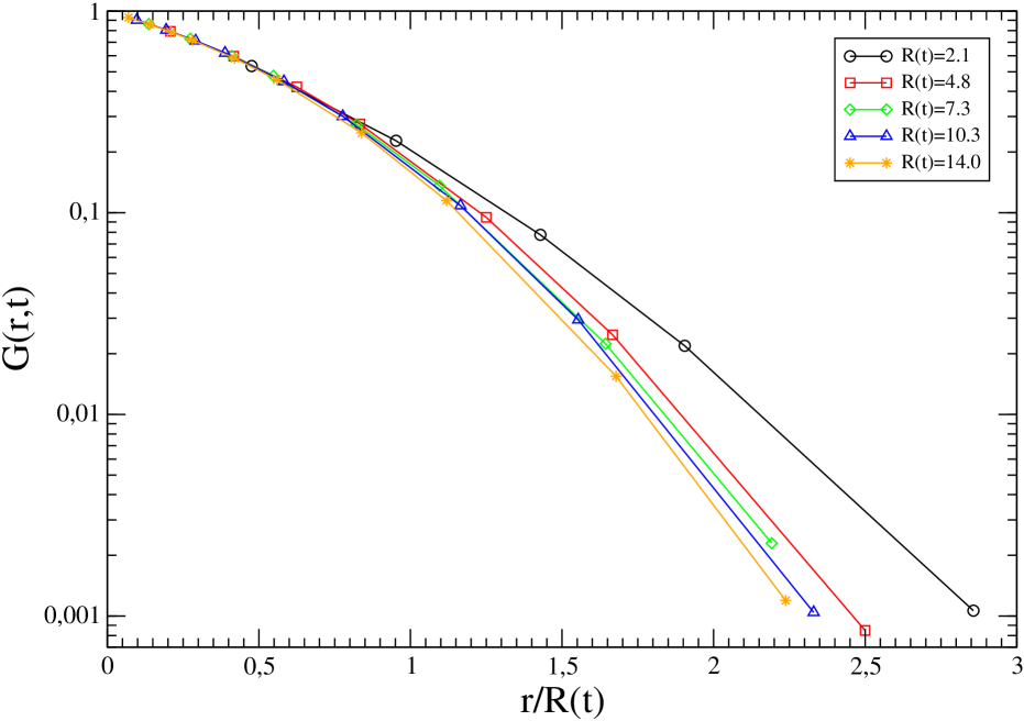
Figure 1: The spin-spin correlation function $G(r,t)$ is plotted against $r/R(t)$ on a log-linear scale for a quench of the clean Ising model to $T_{f}=0$. Different curves correspond to different values of $R(t)$ (see the key), namely of time $t$. The system size is $L=512$. The deviations from collapse at large values of the scaling variable $r/R(t)$ are ascribed to the effects of the approach to critical percolation that has to be taken into account with a second scaling variable, see the text for the explanation of this fact.

An important quantity to assess percolative properties is the pair connectedness function, which in percolation theory is defined as the probability that two points separated by a distance $r$ belong to the same cluster. In two dimensions, random percolation theory at $p=p_{c}$ gives Stauffer ; Saberi ; Christensen

$$C_{perc}(r,r_{0})\sim\left(\frac{r}{r_{0}}\right)^{-2\Delta}$$ (14)

where $r_{0}$ is a reference distance, usually the lattice spacing. Equation (14) holds true for large $r/r_{0}$, with the critical exponent $\Delta=5/48$. The dotted black curve in Fig. 4 is a numerical evaluation of $C_{perc}$ on a square lattice with $r_{0}=1$ and size $L=512$. The curve is indistinguishable from Eq. (14) except at large distances where finite-size effects set in.

In the coarsening system we evaluate this quantity as follows: at a given time, after identifying all the domains of positive and negative spins, the connectivity is computed as

$$C(r,t)=\frac{1}{4L^{2}}\sum_{i}\sum_{i_{r}}\langle\delta_{S_{i},S_{i_{r}}}\rangle,$$ (15)

where $\delta_{S_{i},S_{j}}=1$ if the two spins belong to the same cluster – namely they are aligned and there is a path of aligned spins connecting them – and $\delta_{S_{i},S_{j}}=0$ otherwise.

Another quantity that will be considered is the (average) squared winding angle $\langle\theta^{2}\rangle$. Its definition is the following: At a given time, we chose two points $i,j$ on the external perimeter – the hull – of a cluster and we compute the winding angle $\theta_{ij}$, namely the angle (measured counterclockwise) between the tangent to the perimeter in $i$ and the one in $j$. After repeating the procedure for all the couples of perimeter points at distance $r$ (measured along the hull), taking the square and averaging over the non-equilibrium ensemble, one ends up with $\langle\theta^{2}(r)\rangle$. The behavior of $\langle\theta^{2}(r)\rangle$ is exactly known in $2d$ critical percolation at $p=p_{c}$ Duplantier ; Wilson , where one has

$$\langle\theta^{2}_{perc}(r,r_{0})\rangle=a+\frac{4k}{8+k}\ln\left(\frac{r}{r_{0}}\right),$$ (16)

with $k=6$ and $a$ a non-universal constant. We will compute this same quantity in the coarsening systems upon moving along the hulls of the growing domains (in this case, we will only consider the largest cluster for numerical convenience).

III Numerical results

In this Section we will present the results of our numerical simulations of the kinetic Ising model.

We will start in Sec. III.1 with the clean system since, although in this case percolation effects have been already reported Arenzon07 ; Sicilia07 ; Sicilia09 ; Barros09 ; Olejarz12 ; Blanchard13 ; Blanchard14 , we use here tools, such as the connectivity (15), that were not considered before. This case, therefore, serves not only to compare with the disordered systems considered further on, but also as a benchmark for these new quantities.

We will then turn to the behavior of the disordered models in Sec. III.2. Let us remark that the very slow growth of $R(t)$ in such systems as compared to the clean case (see Fig. 2) introduces severe limitations to the range of values of $R(t)$ than can be accessed. In particular, choosing large values of $t_{p}$ (meaning large system sizes, see Eq. (3)) would prevent one to access the region with $t\gg t_{p}$ (or, equivalently, $R_{p}(t)\gg L$), the one in which we are mainly interested in, where the percolation structure has been fully established. For this reason we will always work with small or moderate values of $L$. In order to compare the clean system to the disordered ones in the same regimes, the same choice will be made for the pure system.

All the results contained in this Section are obtained with periodic boundary conditions by averaging over a non-equilibrium ensemble with order $10^{5}-10^{6}$ of realisations. The system linear size is $L=512$ in units of the lattice spacing.

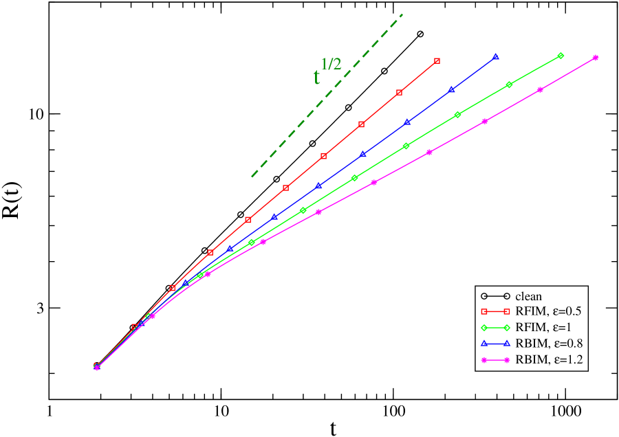
Figure 2: The growing length $R(t)$ is plotted against time on a log-log scale for the different models considered in this paper and for different values of the disorder strength $\epsilon$ (see the key). The dashed green line is the asymptotic behavior $t^{1/2}$ expected for the clean case.

III.1 Clean case

Let us consider a quench of the clean Ising model to $T_{f}=0$. The wrapping cluster that develops around $t_{p}$ can cross the system in different ways. The first possibility is to span the system from one side to the other horizontally or vertically. We denote the probabilities of such configurations as $\pi_{1,0}$ and $\pi_{0,1}$, respectively. Obviously, for a lattice with unit aspect ratio, $\pi_{0,1}=\pi_{1,0}$. Another possibility is to have a domain traversing the sample in both the horizontal and the vertical direction, the probability of which we indicate $\pi_{0,0}$. Finally, clusters can percolate along one of the two diagonal directions with equal probabilities $\pi_{1,-1}$ and $\pi_{-1,1}$. Since we operate with periodic boundary conditions, other wrapping shapes – winding the torus more than once – are also possible but these will not be considered in the following since they occur with an extremely small probability. The quantities mentioned above are exactly known for two-dimensional critical percolation. They are Pinson

$$\pi_{0,1}+\pi_{1,0} \simeq 0.3388\;,$$

$$\pi_{0,0} \simeq 0.61908\;,$$ (17)

$$\pi_{1,-1}+\pi_{1,1} \simeq 0.04196\;.$$

Upon computing the wrapping probabilities defined above during the phase-ordering process and plotting them against $R(t)$ (shown in Fig. 2) we find the curves shown in Fig. 3 (black curves with circles, which perfectly superimpose on the others, represent the clean case at hand).

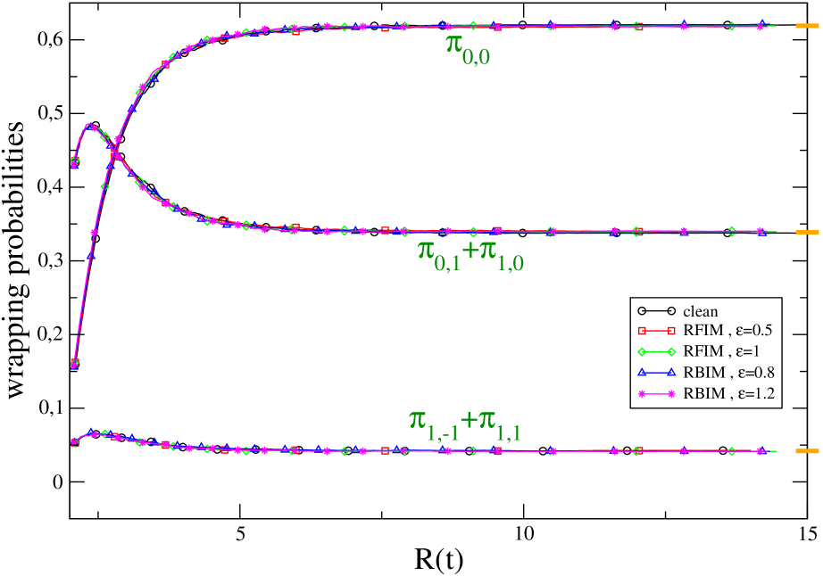
Figure 3: The three wrapping probabilities $\pi_{0,0}$, $\pi_{0,1}+\pi_{1,0}$ and $\pi_{1,-1}+\pi_{1,1}$ are plotted against $R(t)$ for a square lattice system with linear size $L=512$. Each set of superimposing curves represents one of these quantities (as labelled in the figure) for different values of the disorder strength (see the key), including the clean case. The exact values of random percolation are marked with a bold (orange) segment on the extreme right.

A first observation is that any of these quantities, starting from zero immediately after the quench ($R(t)\simeq 0$) – since as already mentioned there cannot be any crossing in the initial state – saturate at long times (large $R(t)$) to values which are very precisely consistent with those given in Eq. (17) of critical percolation (bold orange segment on the far right). This fact was first pointed out in Barros09 ; Olejarz12 . The second observation is that all these probabilities attain their asymptotic values around a certain $R(t)$ that can be used as a rough estimation of $R(t_{p})$. Concretely, it occurs at $R(t)\gtrsim 5$. Repeating the numerical experiment in systems with different sizes, indeed, one can check that this determination of $R(t_{p})$ increases with $L$, as it is expected after Eq. (5).

The next quantity we consider is the pair connectedness defined in Eq. (15). In Fig. 4 we plot this quantity against $r$ for different values of $R(t)$, namely of time measured with the relevant clock (black curves with circles, which perfectly superimpose with the others, represent the clean case at hand). The area $S(t)=\sum_{r}C(r,t)$ below the curves increases as time elapses, because $S(t)$ is the probability that two points chosen at random in the system belong to the same cluster, and the number of domains decreases during coarsening. Regarding the form of each curve, after a first transient that we identify as $t\lesssim t_{p}$, one observes the typical power-law behavior of critical percolation, Eq. (14) (dotted black line). This, however, is only true for values of $r$ larger than a certain time-dependent value. This can be explained as due to the fact that on scales smaller than $R(t)$ correlations set in and domains get compact. It is therefore natural to observe the percolative behavior only at distances larger than $R(t)$.

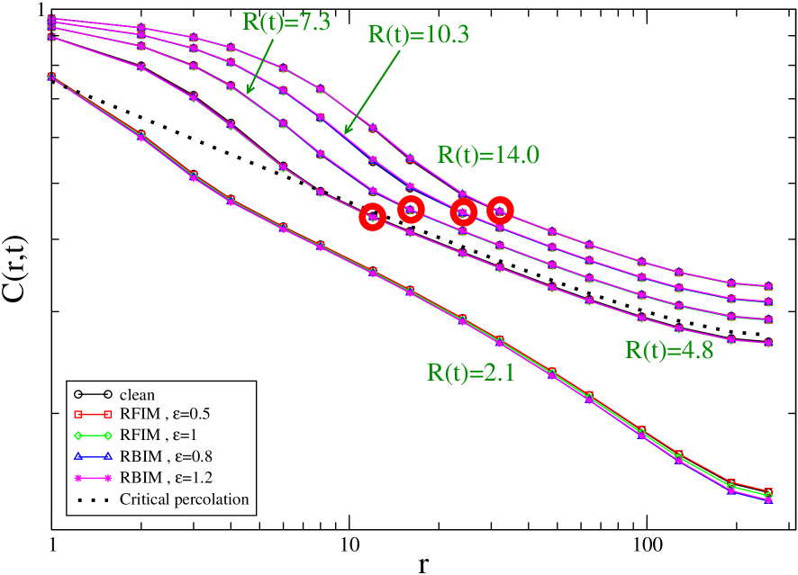
Figure 4: The connectedness $C(r,t)$ is plotted against $r$. Each set of superimposing curves represents this quantity for a given value of $R(t)$ ($R(t)=2.1,4.8,7.3,10.3,14.0$, from bottom to top, as indicated in the figure) for different values of the disorder strength (see the key), including the clean case (black curves with circles). The same quantity computed numerically in a random percolation square lattice at $p=p_{c}$ is represented by the dotted black curve, which agrees with the exact form (14) apart from some finite size effects at large $r$. The red circles correspond to the point where the percolative behavior starts to be observed.

Let us now discuss the properties of $C$ more quantitatively, concerning in particular its scaling behavior. According to the discussion around Eq. (13) we expect a two-parameter scaling to hold also for the pair connectivity, namely

$$C(r,t)=c\left(\frac{r}{R(t)},\frac{L}{R_{p}(t)}\right),$$ (18)

where $c$ is a scaling function. In order to make the discussion simpler, let us start by discussing the scaling properties for times much longer than the one – $t_{p}$ – where the percolating structure sets in. This means that the second entry in Eq. (18) is small and one has

$$C(r,t)\simeq c\left(\frac{r}{R(t)},0\right)={\cal C}\left(\frac{r}{R(t)}\right),$$ (19)

where ${\cal C}$ is a single-variable scaling function. One can infer the form of the scaling function ${\cal C}(x)$ for large values of $x$ as follows. After $t_{p}$ the system has percolative properties for $r>R(t)$, and it can be thought of as a percolation problem on a lattice with spacing $R(t)$, for which Eq. (14) must hold with the replacement $r_{0}\to R(t)$, namely

$$C(r,t)\sim\left(\frac{r}{R(t)}\right)^{-2\Delta}\hskip 28.45274pt\mbox{for}\quad r\gg R(t).$$ (20)

In order to match Eqs. (19) and (20) it must be

$${\cal C}(x)\simeq x^{-2\Delta}\hskip 28.45274pt\mbox{for}\quad x\gg 1.$$ (21)

In the opposite situation of small distances $r\ll R(t)$ we are exploring the properties of the domains well inside their correlated region, where there is no percolative structure and the scaling function $c$ decays faster. All the above holds for $t\gg t_{p}$ where the second entry in the scaling function of Eq. (18) is very small. In the opposite situation $t\ll t_{p}$ (but $t$ larger than the microscopic time $t_{0}$ when scaling sets in) one has

$$C(r,t)\simeq c\left(\frac{r}{R(t)},\infty\right)=\Xi\left(\frac{r}{R(t)}\right).$$ (22)

For $r\gg R(t)$ the scaling function $\Xi$ is expected to be different from ${\cal C}$, because these two functions describe two contrasting situations where the percolative structure is, respectively, absent or present. For $r\ll R(t)$, instead, the scaling function $\Xi$ should be akin to ${\cal C}$, because in any case the domain structure is shaped by correlations on these short lengthscales.

Let us submit these scaling ideas to the numerical test. In Fig. 5 we plot $C(r,t)$ against $r/R(t)$. We start by discussing the regime of sufficiently long times $t\gg t_{p}$. Considering the previous rough estimate $R(t_{p})\gtrsim 5$ obtained by inspection of the wrapping probabilities (see Fig. 3), we can assume that such a regime can be sufficiently well represented by the curves with $R(t)$ from $R(t)=4.8$ onward in Fig. 5. According to Eqs. (18) we should find collapse of such curves at different times on a unique mastercurve ${\cal C}$, with the behavior (21). The numerical data show indeed superposition, except in a region of large $r$ (which moves towards smaller values of $r$ as time elapses) where data collapse is lost due to finite size effects. Notice also that, from $x\gtrsim x_{perc}=1.6$ the mastercurve behaves as in Eq. (21), as can be checked by comparing the numerical data with the dotted black line. The departure from the behavior (21) at very large $x$ is always flanked by the failure of data collapse, a fact which strengthens the idea that both these effects are due to finite size corrections. Indeed, in the inset in the same figure we plot $(r/R(t))^{2\Delta}C(r,t)$ against $r$ for all data in the main panel except the ones for $R(t)=2.1$. The data collapse onto a master curve that is flat at not so large $r$ and then bends upwards due to finite-size corrections that can be captured by a correcting factor $f(r/L)$ to be added as a factor to the scaling law (20). In the inset we also show the data for actual critical percolation that superimpose on the dynamic data thus confirming that the bending of the curves is not a dynamic effect but just conventional finite-size corrections. Let us now move to the regime with $t\ll t_{p}$. The curves with $R(t)=2.1$ and $R=2.7$ in Fig. 5 are representative of such regime. We find that these two lines do not collapse for all values of $x>x_{perc}$. This is because, since we work with relatively small values of $L$ (the reasons for that having been explained at the beginning of Sec. III) the regime with $R(t)\ll L$ where Eq. (22) holds is not fully reached in our simulations. However it is interesting to observe that in the region $x<x_{perc}$ data collapse is obeyed on a mastercurve $\Xi$ which is almost indistinguishable from ${\cal C}$, as expected according to the discussion below Eq. (22). On the other hand in the region $x>x_{perc}$ a marked difference is observed between the curves with $R\leq 2.7$ and those with $R(t)\geq 4.8$, as due to the fact that the percolative structure is still absent when the former ones are computed whereas it has been established later.

Finally, let us comment on the fact that the quantity $C$, besides being very informative about the twofold properties of the system – compact and correlated at small distances vs fractal and uncorrelated at large distances – is also very well suited to assess the role of the extra growing length $R_{p}(t)$ in determining the scaling properties. Indeed, although in Blanchard14 indications that Eq. (13) reproduces the data for $G$ better than the simple form (1) were given, the deviations from Eq. (1) were relatively small and located in the region of large $r$ where $G$ becomes very small. Instead, as Fig. 5 clearly shows, a simple scaling form for $C$ completely fails in describing the data, due to the differences between ${\cal C}$ and $\Xi$ in the region $x>x_{perc}$. For this quantity the improvement of Eq. (18) over a single parameter scaling is conspicuous.

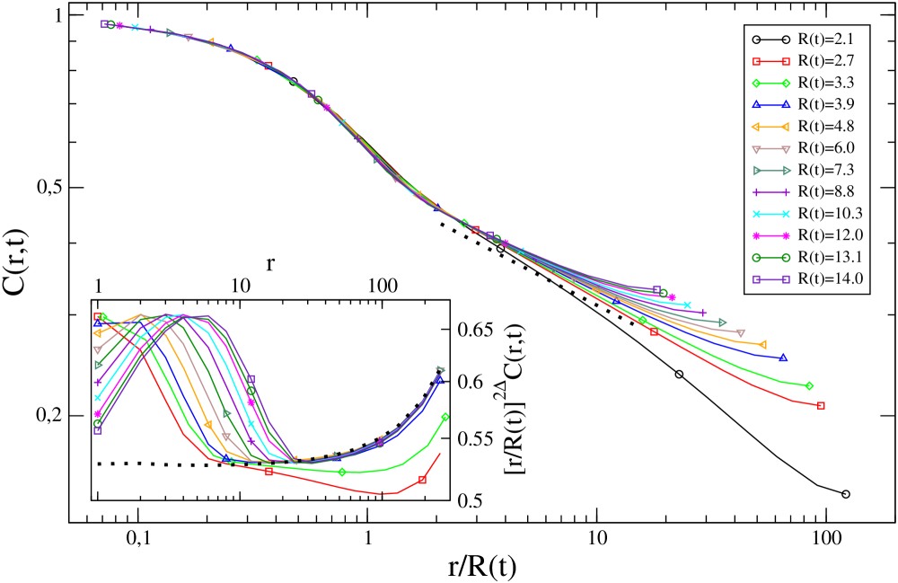
Figure 5: The connectedness $C(r,t)$ against $r/R(t)$ in the clean case, for different values of $R(t)$ (see the key) showing conventional scaling for short lengths compared to $R(t)$. The dotted black line is the behavior (21). In the inset, $(r/R(t))^{2\Delta}C(r,t)$ is plotted against $r$. The dotted black line is the same curve as in Fig. 4, namely the connectedness function computed numerically in a random percolation square lattice at $p=p_{c}$. The curves fail to scale on short lengths now but the plot demonstrates that the the long lengths behave as in critical percolation.

The last quantity that we will consider is the winding angle, that is plotted in Fig. 6 (the clean case corresponds to the black lines with circles, which are perfectly superimposed to the others), for various choices of $R(t)$.

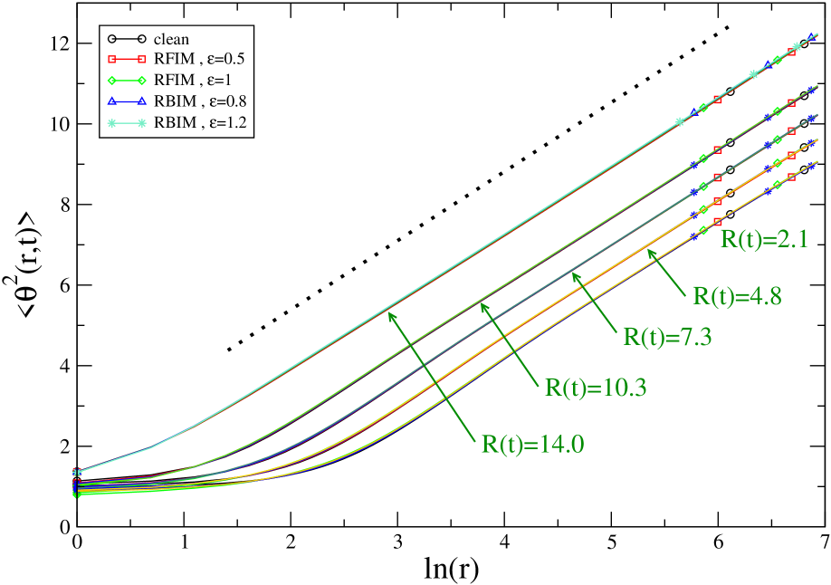
Figure 6: The winding angle $\langle\theta^{2}(r,t)\rangle$ is plotted against $\ln r$. Each set of superimposing curve represents this quantity for different values of the disorder strength (see the key), including the clean case. The exact form (16) of random percolation is the dotted black curve (the constant $a$ is arbitrarily fixed to be $a=2$).

Following the discussion relative to the connectivity, for $t>t_{p}$ we expect to observe the percolative behavior of Eq. (16), with the replacement $r_{0}\to R(t)$, namely Duplantier ; Wilson

$$\langle\theta^{2}(r,t)\rangle=a+\frac{4k}{8+k}\ln\left(\frac{r}{R(t)}\right),$$ (23)

for $r\gg R(t)$. If this is true we ought to find data collapse of the curves for $\langle\theta^{2}(r,t)\rangle$ at different times upon plotting them against $r/R(t)$, if $r\gg R(t)$ is large enough and $R(t)\gg R(t_{p})$ (similarly to what previously observed for $C(r,t)$, see Fig. 5). In addition, the mastercurve should be the one of Eq. (23) for $r$ sufficiently larger than $R(t)$. This kind of plot is shown in Fig. 7. Interestingly, not only we observe data collapse on the mastercurve (23) when $t\gg t_{p}$, but this occurs with good precision also for a value $R(t)=2.1$ which was shown in Fig. 5 to be representative of a situation with $t<t_{p}$. This implies that, for this particular quantity, a single parameter scaling

$$\langle\theta^{2}(r,t)\rangle={\cal T}\left(\frac{r}{R(t)}\right),$$ (24)

where ${\cal T}(x)$ is a scaling function, accounts for the data. This does not contradict the general fact that – due to the existence of the extra-length $R_{p}$ – a two-parameter scaling has to be expected. Indeed Eq. (24) is a particular case of a two-parameter form

$$\langle\theta^{2}(r,t)\rangle=\Theta^{2}\left(\frac{r}{R(t)},\frac{L}{R_{p}(t)}\right),$$ (25)

where $\Theta^{2}$ is a scaling function with a weak dependence on the second entry.

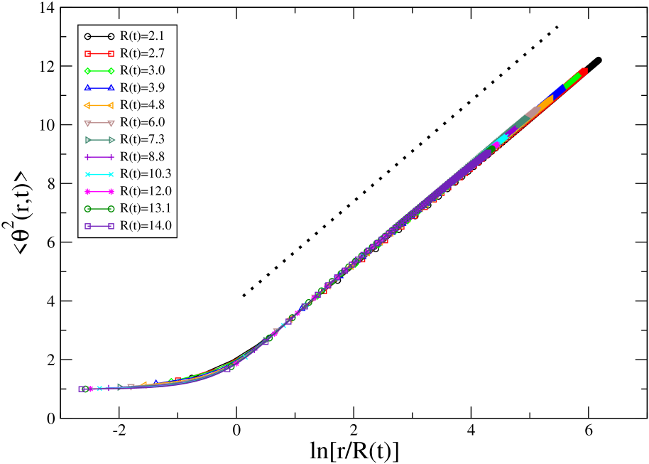
Figure 7: The winding angle $\langle\theta^{2}(r,t)\rangle$ is plotted against $\ln\left[r/R(t)\right]$ for the pure case. The exact form (16) of random percolation is the dotted black curve (the constant $a$ is arbitrarily fixed to be $a=4$).

III.2 Quenched disorder

In this Section we will discuss the effects of quenched disorder on the approach to percolation by considering the dynamics of the RFIM and the RBIM. We will investigate the properties of the same quantities analyzed in the clean limit in Sec. III.1.

Before starting this analysis let us briefly overview what is known about the coarsening behavior of weakly disordered models. When weak disorder is added, the growth law $R(t)$ is markedly slowed down with respect to its growth in the pure case. This is observed in the RFIM and in the RBIM as well. In particular, in the low temperature limit we are considering in this paper (i.e. $T\to 0$ with fixed $\epsilon$, see the discussion around Eq. (11)), after a microscopic time, a regime in which an effective algebraic law, $R(t)\sim t^{1/\zeta(\epsilon)}$, is entered. The effective growth exponent, starting from the value $\zeta(\epsilon=0)=2$ of the clean case, monotonously increases with $\epsilon$ Paul07 ; Kolton . This shows that in this stage $R(t)$ grows slower in the disordered models than in the clean case. All these features are quite neatly observed in Fig. 2, where the behavior of $R(t)$ is shown. At rather long times, for $t\gg t_{cross}$, a crossover occurs to an even slower growth, with $R(t)$ increasing logarithmically, representing the asymptotic behavior Fisher88 ; Kolton . The simulations presented in this paper will never enter such an asymptotic stage, they will be restricted to $t<t_{cross}$.

The slowing down of $R(t)$ reflects a fundamental difference in the coarsening mechanisms at $\epsilon=0$ and $\epsilon\neq 0$. In the clean system phase-ordering proceeds by softening and flattening of interfaces, which is promoted by surface tension and is a non-thermal effect. This means that activated processes are irrelevant and, as a consequence, the kinetics has the same basic features at any $T_{f}$, including $T_{f}=0$ (which is indeed the case presented in the previous Section). On the other hand, as soon as some disorder – no matter how small – is present, interfaces get stuck in pinned configurations and the evolution can only be promoted by thermal activation. These systems are frozen at $T_{f}=0$ (this is why we work at finite, although vanishing small, temperatures $T_{f}\to 0$).

The basic result of this Section is that, despite the dynamics in the presence of disorder being fundamentally different from the ones of the pure case, notwithstanding the fact that $R(t)$ increases in a radically different way, the percolative features observed in the clean case occur with the same qualitative and quantitative modality in the presence of disorder. Moreover, this occurs both for random fields and random bonds.

In order to prove the statement in the previous paragraph, let us start by discussing the behaviour of the crossing probabilities introduced at the beginning of Sec. III.1. These quantities are plotted in Fig. 3. For both the RFIM and the RBIM and for any strength of disorder considered parametrized by $\epsilon$ these probabilities are basically indistinguishable from those of the clean $\epsilon=0$ case. This shows that the effect of disorder does not spoil the occurrence of the percolative structure, nor how and when (provided time is parametrized in terms of $R$) it is formed. As a byproduct, the independence of the crossing probabilities on $\epsilon$ implies that Eq. (6) is valid beyond the pure case with a unique value of the exponent $z_{p}/z_{d}$, at least for the non-conserved order parameter dynamics on the square lattice considered here. Let us mention that, since $R(t)$ is strongly $\epsilon$-dependent, we should not find the nice collapse of Fig. 3 if we plotted against time, instead of against $R(t)$. Equation (6) would not look $\epsilon$-independent upon expressing $R_{p}$ as a function of time either, namely in the form of Eq. (3). This shows that the typical size of correlated domains is the natural parametrization of time in this problem. It will also help us conclude about the system size dependence of the percolation time $t_{p}$ without having to simulate different system sizes, as we will explain below.

Let us move on to the connectedness function. A comparison between the clean case and the disordered ones is presented in Fig. 4. In this figure one sees that all the disordered cases fall onto the clean case provided that times are chosen in order to have the same growing length. For instance, the curve for $t=103$ without disorder is indistinguishable from the one at $t=1446$ for the RBIM with $\epsilon=1.2$, because at these times the size $R(t)$ of the domains in the two models is the same, $R(t)=14.0$ (last curve on the top in Fig. 4). Notice that collapse of the various curves is obtained for the RFIM and the RBIM, and for any strength $\epsilon$ of disorder. This confirms that the way in which the percolation structure develops, and the scaling properties associated to that, are those discussed in the previous Section regarding the clean case, and are largely independent of the presence of disorder.

Finally, we arrive at the same conclusion by considering the winding angle. This quantity is shown in Fig. 6 where the clean system and different disordered cases are shown. As in Fig. 4, the comparison is made by choosing times so as to have the same $R(t)$. Also in this case one observes an excellent superposition of all curves, further supporting the conclusion that the presence of disorder does not modify the percolative properties observed in the clean case. As a byproduct, this also mean that a scaling plot like the one presented in Fig. 7 for the pure case would look the same if data for the disordered models were used. This implies that the scaling properties discussed in the previous Section for the winding angle apply in the presence of quenched disorder as well. The same holds for the connectedness function.

As a final important point, let us discuss the role of the crossover time $t_{cross}$ where the growth law turns to a logarithmic form. As we said at the beginning of this Section, our simulations do not even approach times of the order $t_{cross}$. However, the existence of this crossover time is associated to a further characteristic length $\lambda(\epsilon)=R(t_{cross})$ which might be relevant to the scaling properties discussed in Sec. III.1. Indeed, considering the connectedness function for example, the dependence on $\lambda$ is expected to enter a scaling form in the following way

$$C(r,t)=c\left(\frac{r}{R(t)},\frac{L}{R_{p}(t)},\frac{R(t)}{\lambda(\epsilon)}\right),$$ (26)

where for simplicity we use the same symbol $c$ also for this new, three entry, scaling function. Clearly, since in the range of times considered in our simulations we have $t\ll t_{cross}$, and consequently $R(t)\ll\lambda(\epsilon)$, the last entry in the above equation is always around zero and can be neglected. This, in turn, makes our results independent of disorder $\epsilon$, as we have already discussed, a fact that has been called superuniversality Fisher88 . Notice that this does not mean that disorder is ineffective, since the growth law $R(t)$ changes dramatically due to the quenched randomness. However, it is quite natural to expect that such insensitivity of $c$ on $\epsilon$ could be spoiled if times where pushed to such late regimes as to give $R(t)\gtrsim\lambda(\epsilon)$. In this case the last entry in Eq. (26) could start, in principle, to play a role, introducing an $\epsilon$-dependence and spoiling the superuniversality we have shown to hold in the regime accessed in our simulations. The investigation of such a late regime requires a huge numerical effort that is beyond the scope of this paper and remains a challenge for future research.

IV Conclusions

In this paper we have investigated the relevance of percolative effects on the phase-ordering kinetics of the two-dimensional Ising model quenched from the disordered phase to a very low final temperature. We have considered the clean case as a benchmark, and two forms of quenched randomness, random bonds and random fields. The presence and the properties of the percolation cluster have been detected by inspection of quantities, such as the pair-connectedness, that represent an efficient tool to detect the percolative wrapping structure hidden in the patchwork of growing domains.

The main finding of this paper is that the addition of weak quenched randomness, while sensibly changing the speed of the ordering process, does not impede the occurrence of percolation, nor it changes the way in which it sets in, even at a quantitative level. Indeed, we find that quantities such as the wrapping probabilities, the connectivity function and the winding angle behave in the same way with great accuracy for any choice of the disorder strength, including the clean case, once time has been measured in units of the size $R(t)$ of the ordered regions.

All the above can be accounted for in a scaling framework where coarsening, percolation and disorder are associated to three characteristic lengths, $R$, $R_{p}$, and $\lambda$ respectively, and the interplay between them depends on how such lengths compare between them and with the linear system size.

The results in Sicilia08 and in this paper show that the relevance of percolation, which was previously pointed out for $2d$ clean systems, extends to the much less understood realm of disordered systems, making this issue of a quite general character. This not only opens the way to further studies on more general disordered systems (for instance, randomly diluted models where a more complex scaling structure has been recently observed Corberi13 ), but also prompts the attention on a possible generalisation of analytical theories where the properties of phase-ordering are traced back to percolation effects, originally developed for clean systems, to the disordered cases.

Acknowkledgements F. Corberi and F. Insalata thank the LPTHE Jussieu for hospitality during the preparation of this work. L. F. Cugliandolo is a member of Institut Universitaire de France, and she thanks the KITP University of California at Santa Barbara for hospitality. This research was supported in part by the National Science Foundation under Grant No. PHY11-25915.

References

- (1) A. J. Bray, Adv. Phys. 43, 357 (1994).
- (2) Kinetics of Phase Transitions, edited by S. Puri and V. Wadhawan, CRC Press, Boca Raton (2009).
- (3) J. J. Arenzon, A. J. Bray, L. F. Cugliandolo, and A. Sicilia, Phys. Rev. Lett. 98, 145701 (2007).
- (4) A. Sicilia, J. J. Arenzon, A. J. Bray, and L. F. Cugliandolo, Phys. Rev. E 76, 061116 (2007).
- (5) A. Sicilia, Y. Sarrazin, J. J. Arenzon, A. J. Bray, and L. F. Cugliandolo, Phys. Rev. E 80, 031121 (2009).
- (6) K. Barros, P. L. Krapivsky, and S. Redner, Phys. Rev. E 80, 040101 (2009).
- (7) J. Olejarz, P. L. Krapivsky, and S. Redner, Phys. Rev. Lett. 109, 195702 (2012).
- (8) T. Blanchard and M. Picco, Phys. Rev. E 88, 032131 (2013).
- (9) T. Blanchard, F. Corberi, L. F. Cugliandolo, and M. Picco, EPL 106, 66001 (2014).
- (10) D. Stauffer and A. Aharony, Introduction to Percolation Theory (Taylor and Francis, London, 1994).
- (11) K. Christensen, Percolation Theory (Imperial College Press, London, 2002).
- (12) A. A. Saberi, Phys. Rep. 578, 1 (2015).
- (13) T. Blanchard, L. F. Cugliandolo, M. Picco, and A. Tartaglia, Critical percolation in bidimensional kinetic spin models, arXiv:16
- (14) J. Cardy and R. M. Ziff, J. Stat. Phys. 110, 1 (2003).
- (15) F. Corberi, Comptes rendus - Physique 16, 332 (2015).
- (16) V. Likodimos, M. Labardi, and M. Allegrini, Phys. Rev. B 61, 14440 (2000).
- (17) V. Likodimos, M. Labardi, X. K. Orlik, L. Pardi, M. Allegrini, S. Emonin, and O. Marti, Phys. Rev. B 63, 064104 (2001).
- (18) H. Ikeda, Y. Endoh, and S. Itoh, Phys. Rev. Lett. 64, 1266 (1990).
- (19) A. G. Schins, A. F. M. Arts, and H. W. de Wijn, Phys. Rev. Lett. 70, 2340 (1993).
- (20) D. K. Shenoy, J. V. Selinger, K. A. Grüneberg, J. Naciri, and R. Shashidhar, Phys. Rev. Lett. 82, 1716 (1999).
- (21) D. S. Fisher, P. Le Doussal, and C. Monthus, Phys. Rev. Lett. 80, 3539 (1998).
- (22) D. S. Fisher, P. Le Doussal, and C. Monthus, Phys. Rev. E 64, 066107 (2001).
- (23) F. Corberi, A. de Candia, E. Lippiello, and M. Zannetti, Phys. Rev. E 65, 046114 (2002).
- (24) M. Rao and A. Chakrabarti, Phys. Rev. E 48, R25(R) (1993).
- (25) M. Rao and A. Chakrabarti, Phys. Rev. Lett. 71, 3501 (1993).
- (26) C. Aron, C. Chamon, L. F. Cugliandolo and M. Picco, J. Stat. Mech. P05016 (2008).
- (27) F. Corberi, E. Lippiello, A. Mukherjee, S. Puri and M. Zannetti, Phys. Rev. E 85, 021141 (2012).
- (28) S. Puri and N. Parekh, J. Phys. A 26, 2777 (1993).
- (29) E. Oguz, A. Chakrabarti, R. Toral, and J.D. Gunton, Phys. Rev.B 42, 704 (1990).
- (30) E. Oguz, J. Phys. A 27, 2985 (1994).
- (31) R. Paul, S. Puri, and H. Rieger, Europhys. Lett. 68, 881 (2004).
- (32) R. Paul, S. Puri, and H. Rieger, Phys. Rev. E 71, 061109 (2005).
- (33) R. Paul, G. Schehr, and H. Rieger, Phys. Rev. E 75, 030104 (2007).
- (34) F. Corberi, E. Lippiello, A. Mukherjee, S. Puri, and M. Zannetti, J. Stat. Mech.: Theory and Experiment P03016 (2011).
- (35) M. Henkel and M. Pleimling, Europhys. Lett. 76, 561 (2006).
- (36) M. Henkel and M. Pleimling, Phys. Rev. B 78, 224419 (2008).
- (37) J. H. Oh, and D. Choi, Phys. Rev. B 33, 3448 (1986).
- (38) F. Corberi, R. Burioni, E. Lippiello, A. Vezzani, and M. Zannetti, Phys. Rev. E 91, 062122 (2015).
- (39) M. F. Gyure, S. T. Harrington, R. Strilka, and H. E. Stanley, Phys. Rev. E 52, 4632 (1995).
- (40) S. Puri, D. Chowdhury, and N. Parekh, J. Phys. A 24, L1087 (1991).
- (41) S. Puri, D. Chowdhury, and N. Parekh, J. Phys. A 24, L1087 (1991).
- (42) S. Puri and N. Parekh, J. Phys. A 25, 4127 (1992).
- (43) A. J. Bray and K. Humayun, J. Phys. A 24, L1185 (1991).
- (44) B. Biswal, S. Puri, and D. Chowdhury, Physica A 229, 72 (1996).
- (45) R. Paul, G. Schehr, and H. Rieger, Phys. Rev. E 75, 030104(R) (2007).
- (46) H. Park and M. Pleimling, Phys. Rev. B 82, 144406 (2010).
- (47) F. Corberi, E. Lippiello, A. Mukherjee, S. Puri and M. Zannetti, Phys. Rev. E 88, 042129 (2013).
- (48) C.Castellano, F.Corberi, U.Marini Bettolo Marconi and A.Petri, Journal de Physique IV 8,93 (1998).
- (49) A. Sicilia, J. J. Arenzon, A. J. Bray, and L. F. Cugliandolo, EPL 82, 10001 (2008).
- (50) F. Corberi, E. Lippiello, and M. Zannetti, J. Stat. Mech., P10001 (2015).
- (51) Y. Imry and S.-k. Ma, Phys. Rev. Lett. 35, 1399 (1975).
- (52) D. S. Fisher and D. A. Huse, Phys. Rev. B 38, 373 (1988).
- (53) J. L. Iguain, S. Bustingorry, A. B. Kolton, and L. F. Cugliandolo, Phys. Rev. B 80, 094201 (2009).
- (54) H. Pinson, J. Stat. Phys. 75, 1167 (1994).
- (55) B. Duplantier and H. Saleur, Phys. Rev. Lett. 60, 2343 (1988).
- (56) B. Wieland and D. B. Wilson, Phys. Rev. E 68, 056101 (2003).