Conformal field theory of critical Casimir forces between surfaces with alternating boundary conditions in two dimensions

Abstract

Systems as diverse as binary mixtures and inclusions in biological membranes, and many more, can be described effectively by interacting spins. When the critical fluctuations in these systems are constrained by boundary conditions, critical Casimir forces (CCF) emerge. Here we analyze CCF between boundaries with alternating boundary conditions in two dimensions, employing conformal field theory (CFT). After presenting the concept of boundary changing operators, we specifically consider two different boundary configurations for a strip of critical Ising spins: (I) alternating equi-sized domains of up and down spins on both sides of the strip, with a possible lateral shift, and (II) alternating domains of up and down spins of different size on one side and homogeneously fixed spins on the other side of the strip. Asymptotic results for the CCF at small and large distances are derived. We introduce a novel modified Szegö formula for determinants of real antisymmetric block Toeplitz matrices to obtain the exact CCF and the corresponding scaling functions at all distances. We demonstrate the existence of a surface Renormalization Group flow between universal force amplitudes of different magnitude and sign. The Casimir force can vanish at a stable equilibrium position that can be controlled by parameters of the boundary conditions. Lateral Casimir forces assume a universal simple cosine form at large separations.

I Introduction

Van der Waals interactions or more generally Casimir forces are ubiquitous in nature Parsegian (2005). They originate from a confinement or modification of fluctuations. Those can be quantum fluctuations, as in the quantum electrodynamical (QED) Casimir effect Casimir (1948); Bordag et al. (2009), or thermal order parameter fluctuations in the vicinity of a phase transition where correlation lengths are large, resulting in so-called critical Casimir forces (CCFs) between the confining boundaries de Gennes and Fisher (1978); Krech (1994). Analogies and differences between quantum and thermally induced forces have been reviewed in Ref. Gambassi (2009). The CCF is characterized by a universal scaling function that depends on the ratio of the correlation length and the distance between the confining elements. This function is determined by the universality classes of the critical medium Diehl (1986). Its sign depends on the boundary conditions for the order parameter at the surfaces, and hence the CCF can be attractive or repulsive Abraham and Maciolek (2010); Vasilyev et al. (2011). Controlling the sign of the force is important to myriad applications in design and manipulation of micron scale devices. Experimentally, sign control has been achieved with judicious choice of materials in case of QED Casimir forces Munday et al. (2009), and with appropriate boundary conditions for CCFs in binary mixtures Soyka et al. (2008); Hertlein et al. (2008); Gambassi et al. (2009). In QED, a general theorem shows that there is always attraction between mirror symmetric shapes Kenneth and Klich (2006); Bachas (2007). More generally, a theorem for Casimir forces in QED, similar to Earnshaw’s theorem, rules out the possibility of stable levitation (and consequently force reversals) in most cases Rahi et al. (2010). Contrary to that, the sign of the CCF can be tailored by modifying the shape Bimonte et al. (2015) or the boundary conditions Kleban and Vassileva (1991); Kleban and Peschel (1996) of the confining surfaces. For example, a classical binary mixture can be described by an Ising model where homogeneous surfaces have a preference for one of the two components of the mixture, corresponding to fixed spin boundary conditions ($+$ or $-$). Depending on whether the conditions are like ($++$ or $--$) or unlike ($+-$ or $-+$) on two surfaces, the CCF between them is attractive or repulsive. However, so-called ordinary or free spin boundary conditions are difficult to realize experimentally but can emerge due to renormalization of inhomogeneous conditions as we shall show below Toldin et al. (2013). In general, the required conditions for a sign change remain an open problem for general shapes and boundary conditions.

Experimentally, CCFs can be observed indirectly in wetting films of critical fluids Nightingale and Indekeu (1985), as has been demonstrated close to the superfluid transition of ⁴He Garcia and Chan (1999) and binary liquid mixtures Garcia and Chan (2002). More recently, the CCF between colloidal particles and a planar substrate has been measured directly in a critical binary liquid mixture Hertlein et al. (2008); Soyka et al. (2008). Motivated by their potential relevance to nano-scale devices, fluctuation forces in the presence of geometrically or chemically structured surfaces have been at the focus recently. Chemical surface preparation allows for an adsorption preference for the components of a binary mixture that varies along the surface Sprenger et al. (2006); Tröndle et al. (2009, 2010). The CCF between such inhomogeneous surfaces is determined by the effective boundary conditions at which the surfaces “see” each other. Due to renormalization, the effective boundary conditions depend on the distance between the surfaces. This leads to interesting phenomena such as cross-overs with respect to strength and even sign of the force, a lateral force Nowakowski and Napiorkowski (2014) and pattern formation among colloidal particles near non-uniform substrates. The latter situation has been studied experimentally for spherical colloids Soyka et al. (2008). Due to the possibility that the lipid mixtures composing biological membranes are poised at criticality Veatch et al. (2007); Baumgart et al. (2007), it has been also proposed that inhomogeneities on such membranes are subject to a CCF Machta et al. (2012) which provides an example of a 2D realisation.

Initial studies of CCFs mostly considered highly symmetric shapes and boundary conditions since the computation of these interactions is notoriously difficult. Chemical surface structures (and hence modifications of the boundary conditions) and less symmetric geometric shapes complicate CFFs further but add also to the richness of phenomena that can be expected. The experimentally mostly studied critical Casimir systems belong to the Ising universality class and hence the CCF can be extracted from numerical simulations. This has been done for the simple film geometry with various homogeneous boundary conditions Vasilyev et al. (2007); Hasenbusch (2010); Vasilyev and Dietrich (2013) and for spherical particles Hasenbusch (2013). On the analytical side, mostly mean field methods in combination with the Derjaguin approximation have been used to compute CCFs for various geometries Labbe-Laurent and Dietrich (2016). Conformal field theory (CFT) Belavin et al. (1984); Henkel (2013); Francesco et al. (2012) opens a path to compute CCFs exactly in two dimensional systems at criticality: Casimir forces in a strip are related to the central charge of the CFT Cardy (1986); Kleban and Vassileva (1991); Kleban and Peschel (1996), with appropriate modification for boundaries Cardy (1989). There are results for interactions between circles Machta et al. (2012), needles Vasilyev et al. (2013); Ref. Bimonte et al. (2013) describes a general approach for any compact shapes. Sign changes of CCFs due to wedge like surface structures have been reported very recently Bimonte et al. (2015). These techniques have been applied to the Casimir interaction between two needles immersed in a two-dimensional critical fluid of Ising symmetry Eisenriegler and Burkhardt (2016). A general classification of the sign of the critical Casimir force within 2D CFT’s has been obtained within a similar approach Rajabpour .

Figure 1: A statistical lattice model in a domain with a given shape, and a given set of boundary conditions (${\rm BC}_{1}$, ${\rm BC}_{2}$, ${\rm BC}_{3}$). The dots indicate positions where the boundary condition changes. The system has a linear size $L$, and a UV cutoff $a_{0}$ (here represented as lattice spacing). Sending the UV cutoff to zero, while keeping the global shape fixed, one obtains a system that is well described by a conformal field theory (CFT) in the bulk, with boundary condition changing operators (BCC operators) located at the dots on the boundary. Independent of microscopic details, the predictions of CFT are applicable to all models that fall into the same universality class for $L\gg a_{0}$.

How can one describe a system with changing boundary conditions in CFT? Consider a bounded 2d lattice model at equilibrium. For example, one may think of an Ising or Potts model. Imagine that the boundary shape of the system is fixed, as well as its boundary conditions. Let $L$ be the linear size of the system, and $a_{0}$ a UV cutoff, for example the lattice spacing. Imagine that we were able to tune the UV cutoff without affecting the global shape of the system (Fig. 1). Then one may consider $L/a_{0}$ as a large parameter, and focus on the corresponding expansion of the free energy, which is usually of the form $\mathcal{F}=\alpha_{{\rm bulk}}\frac{L^{2}}{a_{0}^{2}}+\alpha_{{\rm surf.}}\frac{L}{a_{0}}+\dots$ The first two terms reflect the fact that the free energy is extensive (at least for systems with sufficiently short-ranged interactions): they scale with the bulk area and with the length of the boundary. At criticality, it is well-known that the next term in this expansion is universal and may be computed using the powerful machinery of CFT,

$$\mathcal{F}=\alpha_{\rm bulk}\frac{L^{2}}{a_{0}^{2}}+\alpha_{{\rm surf.}}\frac{L}{a_{0}}+\mathcal{F}_{{\rm CFT}}+\ldots\,.$$ (1)

In general, the last term can be decomposed as

$$\mathcal{F}_{{\rm CFT}}\,=\,\zeta\,\log\frac{L}{a_{0}}+\theta[{\rm shape}]\,,$$ (2)

with a logarithmic contribution with coefficient $\zeta$, and some function $\theta[{\rm shape}]$ that does not depend on $L/a_{0}$, but instead is a function of the shape of the system. For example, when the system is a rectangle with sides of length $L$ and $\ell$, then it is a function of the aspect ratio, $\theta=\theta(\ell/L)$. For more complicated shapes, described by more length scales $\ell_{1},\ell_{2},\dots$, it is a function $\theta(\ell_{1}/L,\ell_{2}/L,\dots)$. Importantly, both the coefficient $\zeta$ and the function $\theta$ are universal – meaning that they are independent of the microscopic details of the system (like the lattice constant or UV cutoff $a_{0}$) – and can be computed in CFT.

In the following, we focus on simply connected domains with one boundary. In the simplest case when the boundary condition is the same everywhere along the boundary, it is known that the CFT part $\mathcal{F}_{{\rm CFT}}$ of the free energy is directly proportional to the central charge $c$ of the CFT model, and is insensitive to any other details of the theory. More precisely, $\zeta$ and $\theta[{\rm shape}]$ are both given by $c$ times their value in the free scalar field theory with Dirichlet boundary conditions (the normalization convention for the central charge is such that the free scalar field has $c=1$). The variation with the shape of the domain is given in full generality by the Polyakov-Alvarez formula Polyakov (1981); Alvarez (1983), but we will not need it in what follows. In fact, in this paper we consider only very simple shapes, for which the CFT part of the free energy is well-known. Instead, our main interest is in the contributions to the free energy $\mathcal{F}_{\rm CFT}$ that are induced by changes of the boundary conditions along the boundary. When the boundary condition (BC) changes from ${\rm BC}_{1}$ to ${\rm BC}_{2}$, from ${\rm BC}_{2}$ to ${\rm BC}_{3}$, and so on (Fig. 1), at points $z_{1},\ldots,z_{m}$ along the boundary, the partition function, $Z=(L/a_{0})^{-\zeta}e^{-\theta[{\rm shape}]}$, can be expressed as

$$\frac{Z}{Z_{0}}=\left<\phi_{{\rm BC}_{1}|{\rm BC}_{2}}(z_{1})\phi_{{\rm BC}_{2}|{\rm BC}_{3}}(z_{2})\dots\phi_{{\rm BC}_{n}|{\rm BC}_{1}}(z_{n})\right>.$$ (3)

Here $Z_{0}$ is the partition function when the BC is constant along the boundary, and $Z$ is the partition function of the system with the BC changes. The remarkable thing is that, since the change of BC is a local effect, in the scaling limit it can be encoded as a local operator Cardy (1989), dubbed boundary condition changing (BCC) operator. These operators are primary operators, with a scaling dimension $h_{p}$ that depends on the two boundary conditions ${\rm BC}_{p}$ and ${\rm BC}_{p+1}$. As a consequence, the joint effect of several changes of boundary conditions must take the form of a correlation function of local operators along the boundary. How do such changes of boundary conditions affect the free energy of Eq. (2)? The insertion of BCC operators is reflected in the free energy by

$$\mathcal{F}_{{\rm CFT}}\;\rightarrow\;\mathcal{F}_{{\rm CFT}}\,-\,\log\left<\phi_{{\rm BCC},1}(z_{1})\dots\phi_{{\rm BCC},n}(z_{n})\right>\,,$$ (4)

and, since correlation functions must have the scaling form $\left<\phi_{{\rm BCC},1}(z_{1})\dots\phi_{{\rm BCC},n}(z_{n})\right>\,=\,(L/a_{0})^{-\sum_{j}h_{j}}g(z_{1}/L,\dots,z_{n}/L)$, where $h_{j}$ is the scaling dimension of the BCC operator $\phi_{{\rm BCC},j}$, we see that

$$\zeta\rightarrow\zeta+\sum h_{j}\qquad{\rm and}\qquad\theta\rightarrow\theta-\log g(z_{1}/L,\dots,z_{n}/L)\,.$$ (5)

The calculation of arbitrary correlation functions, and thus of the function $g$, is usually difficult. The purpose of this paper is to exploit a few cases where this can be done exactly. A short account of our results has been published recently Dubail et al. (2016).

The rest of the paper is organized as follows. In the next section we consider a general CFT on a strip with a small number of changes in the boundary conditions, to familiarize the reader with the use of BCC operators. In Sec. III we introduce the model of interest: two boundary configurations of the critical Ising model on a strip with periodically alternating boundary conditions. In that section we derive limiting cases of the CCF from simple arguments. Some facts on Toepliz determinants and a modified Szegö formula for the determinant of real antisymmetric block Toeplitz matrices are presented in Sec. IV. This modified formula allows us the compute the exact CCF for the two boundary configurations of the Ising strip in Sec. V. We conclude in Sec. VI.

II CFT for Casimir forces across a strip with changing boundary conditions

In this section, we consider a general CFT in the strip geometry, with boundary condition changes along the surface. Making use of the fact that, in any CFT, two-point functions and three-point functions are entirely fixed by conformal invariance, the CCF can be computed explicitly, because it follows from the correlation function of BCC operators that enters the free energy, see Eq.(4). We assume that the strip has width $L$ and length $W$ where the latter serves as an IR cutoff that can be considered infinity when computing the free energy density ${\cal F_{\rm CFT}}/W$ (see Fig. 2).

II.1 Identical BCs on both sides

Figure 2: Strip of width $L$ and length $W\gg L$. Here the boundary condition is assumed to be identical on both sides.

It is well-know that the CFT part of the free energy of a rectangle of size $L\times W$ for $W/L\gg 1$ is to leading order

$$\mathcal{F}_{\rm CFT}=-\frac{\pi c}{24}\frac{W}{L}+\dots$$ (6)

where $c$ in the central charge of the CFT, and the dots stand for corrections that vanish when $W/L\rightarrow\infty$. The critical Casimir force per unit length between the two boundaries is then

$$\frac{F}{W}=-\frac{d}{dL}\frac{\mathcal{F}_{\rm CFT}}{W}=-\frac{\pi c}{24L^{2}}\,.$$ (7)

II.2 Insertion of two BCC operators

Now consider a strip where the boundary conditions change from ${\rm BC}_{1}$ to ${\rm BC}_{2}$ at the positions $z=x+iL$ (upper boundary) and $z=x^{\prime}$ (lower boundary), see Fig. 3 The two-point correlation function of the BCC operators with scaling dimension $h$ is fixed by conformal invariance,

$$\left<\phi_{{\rm BC}_{1}|{\rm BC}_{2}}(x+iL)\,\phi_{{\rm BC}_{2}|{\rm BC}_{1}}(x^{\prime})\right>=\frac{1}{\left|\frac{2L}{\pi}\sinh\frac{\pi(x-x^{\prime}+iL)}{2L}\right|^{2h}}\,.$$ (8)

Using Eq. (4), the free energy becomes

$$\mathcal{F}_{\rm CFT} = -\frac{\pi c}{24}\frac{W}{L}+2h\,\log\left|\frac{2L}{\pi}\cosh\frac{\pi(x-x^{\prime})}{2L}\right|\,.$$ (9)

There are some limiting cases that are of primary relevance to the rest of this paper. First, take $x\rightarrow-W/2$ and $x^{\prime}\rightarrow W/2$. This corresponds to boundary condition ${\rm BC}_{2}$ on the upper surface, and ${\rm BC}_{1}$ on the lower surface. In that limit the free energy per unit length is to leading order

$$\frac{\mathcal{F}_{\rm CFT}}{W} = -\left(\frac{c}{24}-h\right)\frac{\pi}{L}\,,$$ (10)

where we have ignored logarithmic corrections. From this result one observes that if the boundary condition is different on both sides, then the critical Casimir force becomes repulsive if $h>c/24$. Interestingly, a strip with one change of boundary conditions on the upper boundary and constant boundary conditions on the lower boundary has the free energy of Eq. (10) with $h$ replaced by $h/2$. This can be easily seen by keeping $x$ finite and taking $x^{\prime}\to W/2\gg x$. Hence, like and unlike boundary conditions contribute with equal weight to the total interaction energy between the surfaces (addivity, see also below).

For distances $L$ large compared to $|x-x^{\prime}|$ (but still small compared to the length $W$), the second term in Eq. (9) has a leading logarithmic dependence on $L$ but is independent of $W$ so that it does not contribute to $\mathcal{F}_{\rm CFT}/W$ in the thermodynamic limit $W\to\infty$. Hence, in that limit the strip appears like a strip with equal boundary conditions on both sides, and the free energy per unit length is given by Eq. (10) with $h=0$. In general, a finite number of boundary changes with a finite distance between them does not change the free energy per unit length for asymptotically large $L$ in the thermodynamic limit.

Figure 3: A strip with two changes of boundary conditions. For better readability we write $\phi_{1|2}$ instead of $\phi_{{\rm BC}_{1}|{\rm BC}_{2}}$.

Another limiting case of interest corresponds to short distance, $L\ll|x-x^{\prime}|$. In that limit one easily sees that the free energy per unit length becomes to leading order

$$\frac{\mathcal{F}_{\rm CFT}}{W} = -\frac{\pi c}{24L}+\frac{\pi h}{L}\frac{|x^{\prime}-x|}{W}\,.$$ (11)

This case illustrates the additivity in short distance limit: The second term contributes to the Casimir potential $\pi h/L$ only over the fraction $|x^{\prime}-x|/W$ of the boundaries where they have different boundary conditions. This dependence of the free energy on the position where the BCs change gives rise to a lateral CCF per unit length, determined by

$$\frac{F_{\rm lat}}{W}=-\frac{d({\cal F}_{\rm CFT}/W)}{dx^{\prime}}=-\,{\rm sgn}\,(x^{\prime}-x)\frac{\pi h}{WL}\,.$$ (12)

This lateral force is constant along the boundaries (up to a sign) and tends to align the two boundaries at $x=x^{\prime}$ so that there are no different boundary conditions facing each other. Of course, for $W/L\to\infty$ this force vanishes since the free energy is extensive in $W$. In that limit, a finite lateral force per unit length could be achieved by a finite density of positions where the boundary conditions change. This situation shall be considered in Sec. III.

II.3 Insertion of three BCC operators

Figure 4: A strip with three changes of boundary conditions.

Next, we consider the situation depicted in Fig. 4, which is a strip with three BCC operators on the boundaries, separating three different boundary conditions. It is well-known that the three-point correlation function is entirely fixed by conformal invariance Henkel (2013); Francesco et al. (2012). For three BCC operators on the boundary of the strip, it is given by

$$\left<\phi_{1|2}(w_{1})\phi_{2|3}(w_{2})\phi_{3|1}(w_{3})\right> = \left(\frac{2L}{\pi}\right)^{-h_{1|2}-h_{2|3}-h_{3|1}}\left|\sinh\frac{\pi(w_{1}-w_{2})}{2L}\right|^{-h_{1|2}-h_{2|3}+h_{3|1}}$$

$$\quad\times\;\left|\sinh\frac{\pi(w_{2}-w_{3})}{2L}\right|^{+h_{1|2}-h_{2|3}-h_{3|1}}\left|\sinh\frac{\pi(w_{3}-w_{1})}{2L}\right|^{-h_{1|2}+h_{2|3}-h_{3|1}}\,.$$

For better readability, we have replaced $\phi_{{\rm BC}_{1}|{\rm BC}_{2}}$ by $\phi_{1|2}$; the scaling dimension of the latter operator is $h_{1|2}$. Formula (II.3) easily follows from combining the conformal map $w\mapsto e^{\frac{\pi}{L}w}$, that sends the strip to the upper half-plane, with the well-known formula for the three-point function in the latter domain Henkel (2013); Francesco et al. (2012).

Again, it is interesting to consider the limit of short distances $L$ (compared to the distances between changes in the boundary conditions). To study this limit we set $w_{1}=x_{1}+iL$, $w_{2}=x_{2}+iL$, $w_{3}=x_{3}$ and assume that $x_{1}<x_{2}$. The free energy can be obtained again from Eq. (4). The result depends on the position of $x_{3}$ on the lower boundary relative to $x_{1}$ and $x_{2}$ on the upper boundary. We find for the free energy per unit length

$$\frac{{\cal F}_{\rm CFT}}{W}=-\frac{\pi c}{24L}+\left\{\begin{array}[]{ll}\frac{\pi}{WL}\left[h_{2|3}(x_{2}-x_{1})+h_{3|1}(x_{1}-x_{3})\right]&{\rm for}\,\,x_{3}<x_{1}<x_{2}\\[10.00002pt] \frac{\pi}{WL}\left[h_{1|2}(x_{3}-x_{1})+h_{2|3}(x_{2}-x_{3})\right]&{\rm for}\,\,x_{1}<x_{3}<x_{2}\\[10.00002pt] \frac{\pi}{WL}\left[h_{1|2}(x_{2}-x_{1})+h_{3|1}(x_{3}-x_{2})\right]&{\rm for}\,\,x_{1}<x_{2}<x_{3}\end{array}\right.\,.$$ (14)

Since the scaling dimensions $h_{j|k}$ are all non negative, the part of the free energy that depends on the positions $x_{j}$ where the boundary conditions change is always positive and hence all boundary changes cost energy. To see which configuration minimizes the free energy when we allow the lower boundary and hence $x_{3}$ to move laterally, we consider the lateral force

$$\frac{F_{\rm lat}}{W}=-\frac{d({\cal F}_{\rm CFT}/W)}{dx_{3}}=-\frac{\pi}{WL}\times\left\{\begin{array}[]{ll}-h_{3|1}&{\rm for}\,\,x_{3}<x_{1}<x_{2}\\[10.00002pt] h_{1|2}-h_{2|3}&{\rm for}\,\,x_{1}<x_{3}<x_{2}\\[10.00002pt] h_{3|1}&{\rm for}\,\,x_{1}<x_{2}<x_{3}\end{array}\right.\,.$$ (15)

In general, the lateral force is discontinuous at the points where the boundary conditions change. It points to the center region between $x_{1}$ and $x_{2}$ when $x_{3}$ is located outside that region so that the lower boundary tends to move $x_{3}$ towards $x_{1}$ or $x_{2}$. This is expected since otherwise there could be an arbitrarily large region where the boundary conditions BC₁ and BC₃ face each other, which would cost an extensive energy. When $x_{3}$ is located in the central region between $x_{1}$ and $x_{2}$, the lateral force tends to align $x_{3}$ with $x_{1}$ when $h_{1|2}>h_{2|3}$ and with $x_{2}$ when $h_{1|2}<h_{2|3}$ (If $h_{1|2}=h_{2|3}$ then there is no lateral force in that center region). So the stable point of minimal energy is either $x_{3}=x_{1}$ or $x_{3}=x_{2}$, depending on the relative magnitude of $h_{1|2}$ and $h_{2|3}$. Again, this is expected physically as the scaling dimensions $h_{j|k}$ measure the energy cost associated with two different boundary conditions facing each other. So if $h_{1|2}>h_{2|3}$ it is more expensive to have BC₁ and BC₂ opposite each other than BC₂ and BC₃ and hence $x_{3}=x_{1}$ minimizes the energy.

III Ising universality class with periodically alternating boundary conditions: general arguments and asymptotic limits

Any critical system in the 2d Ising universality class is described by a CFT with central charge $c=1/2$. It admits three type of conformally invariant boundary conditions, corresponding to fixed ($+$ or $-$) spins and free (f) spins along the boundary. The BCC operators implementing the change $(+,-)$ and $(+,f)$ or $(-,f)$ have dimension $h_{(+,-)}=1/2$ and $h_{(\pm,f)}=1/16$ respectively Cardy (1989). We consider again the strip geometry. Of course, the formulas of the previous section apply, but we would like to generalize them to an extensive number of BCC operators. We are interested in computing the critical Casimir forces between surfaces with periodic chemical patterns. Since these chemical structures realize different boundary conditions for the Ising spins when the model is applied to binary mixtures, here we focus on boundary conditions which alternate periodically. In contrast with usual boundary CFT approaches, this problem requires to consider a finite density of BCC operators. We consider the two following configurations:

• Configuration I: A strip of width $L$ and length $W\gg L$ with periodically alternating fixed spin boundary conditions on both edges with periodicity $a$ and lateral shift $\delta$, as illustrated in Fig. 5. The positions of the $2N$ BCC operators are ($w=x+iy$):

  $$w_{2j}=ja+iL,\qquad\qquad w_{2j+1}=ja+\delta\,,\qquad j=1,\ldots,N=W/a.$$ (16)

  For large $W$ or $N$, we are interested in the CFT part of the free energy per unit length, $\mathcal{F}_{\rm CFT}/W$, as a function of $L$ and of the two dimensionless parameters $a/L$ and $\delta/L$.

  

  Figure 5: Ising strip with boundary configuration I.

  

  Figure 6: Ising strip with boundary configuration II.

• Configuration II: A strip of width $L$ and length $W\gg L$ with homogeneous $+$ spins on the lower boundary and alternating domains of $−$ and $+$ spins of different lengths $a$ and $b$, respectively, on the upper boundary, see Fig. 6. The positions of the $2N$ BCC operators are

  $$w_{2j}=j\;(a+b),\qquad\qquad w_{2j+1}=j(a+b)+a\,,\qquad j=1,\ldots,N=W/(a+b)\,.$$ (17)

  Now the CFT part of the free energy per unit length, $\mathcal{F}_{\rm CFT}/W$, is a function of $L$, and of the dimensionless ratios $a/L$ and $b/L$.

III.1 Casimir interaction for small $L\ll a,b,\delta$

When $L$ is much smaller than the separations between boundary changes, we can use the additivity property demonstrated in the previous section.

III.1.1 Configuration I

In the short distance limit one has a very narrow strip, with segments that have ($+$,$-$) boundary conditions on either sides over a fraction $\delta/a$ of the system, and ($+$,$+$)/($-$,$-$) boundary conditions over a fraction $1-\delta/a$. Hence, additivity yields

$$\frac{{\cal F}_{\rm CFT}}{W} = -\frac{\pi c}{24\,L}\left(1-\frac{\delta}{a}\right)-\frac{\pi}{L}\left(\frac{c}{24}-h_{(+,-)}\right)\frac{\delta}{a}+\ldots$$ (18)

$$= -\frac{\pi}{48\,L}+\frac{\pi}{2\,L}\frac{\delta}{a}+\ldots\,,$$

where we used $c=1/2$ and $h_{(+,-)}=1/2$. There is also a logarithmic contribution to $\mathcal{F}_{\rm CFT}$, which reads $\frac{2W}{a}h_{(+,-)}\log(L/a_{0})$ with $a_{0}$ a UV cutoff that does not appear in the force after taking the derivative with respect to $L$. However the latter is subleading in the regime $L\ll a,b$, so we dropped it.

III.1.2 Configuration II

Now the narrow strip has segments ($+$,$-$) boundary conditions over a fraction $a/(a+b)$ of the system, and ($+$,$+$) boundary conditions over a fraction $b/(a+b)$, yielding

$$\frac{{\cal F}_{CFT}}{W} = -\frac{\pi c}{24\,L}\frac{b}{a+b}-\frac{\pi}{L}\left(\frac{c}{24}-h_{(+,-)}\right)\frac{a}{a+b}+\ldots$$ (19)

$$= -\frac{\pi}{48\,L}\frac{b-23a}{a+b}+\ldots,$$

where we again used additivity. Interestingly, the force changes sign depending on the relative amount of $+$ and $-$ spins on the boundaries, and it vanishes to leading order for $a=b/23$. As in the case of Configuration I, we dropped the logarithmic term, which is subleading.

III.2 Asymptotic Casimir interaction for large $L\gg a,b,\delta$ from renormalization group arguments

III.2.1 Configuration I

When $L\gg a$, it is useful to look at each of the two boundaries of the strip from a coarse-grained perspective. Contrary to homogeneous boundary conditions, in this configuration the BCC operators break the scale invariance at the boundaries, because they are associated with the length scale $a$. However, at length scales much larger than $a$, one should be able to regard the coarse-grained boundary as homogeneous, with some new effective boundary condition. The effective boundary condition must be a Renormalization Group (RG) fixed point Diehl (1997). To calculate the free energy for Configuration I, it is not necessary to know what RG fixed point this is exactly, because it clearly has to be the same boundary condition on both sides, so it is given by Eq. (6), with $c=1/2$,

$$\frac{\mathcal{F}_{CFT}}{W}=-\frac{\pi}{48}\frac{1}{L}\,.$$ (20)

We shall see in Sec. V that this result is indeed recovered from the exact solution of the model.

III.2.2 Configuration II

Repeating the same RG argument as for configuration I, we now need to have a finer understanding of the boundary conditions that are RG fixed points. For the Ising universality class, they are expected to be one of the three known conformally invariant boundary conditions Cardy (1989): free (f), or fixed ($+$), ($-$) boundary conditions. We thus need to distinguish the following cases. When $a=b$, the effective boundary condition at large scale should be the free (f) boundary condition. Indeed, since in that case the proportion of $+$ and $-$ spins along the boundary is the same, the effective boundary condition must enjoy $\mathbb{Z}_{2}$-invariance, which rules out fixed boundary conditions. However, when $b>a$, there are more $+$ spins than $-$ spins on the upper boundary, so the $\mathbb{Z}_{2}$-symmetry is broken, and one expects the system to renormalize towards fixed ($+$) boundary conditions. Similarly, for $a>b$, one should obtain fixed ($-$) boundary conditions. Since the lower boundary has homogeneous ($+$) boundary conditions, the CFT free energy must behave asymptotically for $W\gg L\gg a,b$ as

$$\frac{{\cal F}_{CFT}}{W}=\left\{\begin{array}[]{lll}-\frac{\pi}{L}\frac{c}{24}=-\frac{\pi}{L}\frac{1}{48}&\text{if}\quad b>a&(+,+)\;{\rm BC}\,,\\[10.00002pt] -\frac{\pi}{L}\left(\frac{c}{24}-h_{(f,+)}\right)=+\frac{\pi}{L}\frac{1}{24}&\text{if}\quad a=b&(f,+)\;{\rm BC}\,,\\[10.00002pt] -\frac{\pi}{L}\left(\frac{c}{24}-h_{(-,+)}\right)=+\frac{\pi}{L}\frac{23}{48}&\text{if}\quad a>b&(-,+)\;{\rm BC}\,.\end{array}\right.$$ (21)

Since the three possible surface RG fixed points ($+$, $-$ or f) are realized in configuration II, it is interesting to study the RG flow between them. While we shall look at this in greater detail in Sec. V, we present here simple scaling arguments for perturbations of the boundary condition around the free (f) boundary fixed point. We thus start from the case $a=b$, which corresponds effectively to free (f) boundary condition on the upper edge. The action $S$ on the strip can be formally decomposed as

$$S=S_{\text{bulk}}+S_{\text{top edge}}+S_{\text{bottom edge}}\,.$$ (22)

To perturb this boundary condition, one can add a field to the top edge,

$$S_{\text{top edge}}\to S_{\text{top edge}}+\lambda\int dx\;\phi(x),$$ (23)

where $\phi(x)$ is a local operator on the edge, with scaling dimension $h_{\phi}$. For $b$ close to $a$, the coupling constant $\lambda$ must vary linearly with $a-b$. One can see from the action (23) that $\lambda$ has scaling dimension $1-h_{\phi}$, so it must scale as $\lambda\sim(a/b-1)(a+b)^{h_{\phi}-1}$. Thus, there is a natural length scale $\xi_{c}$ with

$$\xi_{c}(\tau)\sim|\tau|^{\frac{1}{h_{\phi}-1}}(a+b),\qquad\tau=a/b-1\,.$$ (24)

At length scales smaller than $\xi_{c}$, the boundary condition is effectively free, and at scales larger than $\xi_{c}$, it is effectively fixed. We will refer to $\xi_{c}$ as the crossover length. Here, for the Ising universality class, we need to determine the perturbing operator $\phi$ that generates an RG flow from free to fixed boundary conditions and its scaling dimension $h_{\phi}$. Clearly, the most natural candidate for that operator is the spin operator itself, which breaks $\mathbb{Z}_{2}$ symmetry. At the boundary, it has scaling dimension $h_{\phi}=1/2$ Cardy (1989), so we obtain a crossover scale and an associated critical exponent $\nu_{c}$, given by

$$\xi_{c}(\tau)\sim|\tau|^{-\nu_{c}}(a+b),\quad\qquad\nu_{c}=2\,.$$ (25)

This length scale determines the scaling of the free energy which is always a function of $L$ and of two dimensionless parameters, which we can chose as $(a+b)/L$ and $\xi_{c}/L$. We are interested in the regime where $L,\xi_{c}\gg a,b$, such that

$${\cal F}_{{\rm CFT}}(L,(a+b)/L,\xi_{c}/L)\;\underset{L,\xi_{c}\gg a,b}{\sim}\;{\cal F}_{{\rm CFT}}(L,0,\xi_{c}/L),$$ (26)

leaving a function of two parameters only. It must take a scaling form, in terms of a universal function $\vartheta$,

$$\frac{{\cal F}_{{\rm CFT}}(L,0,\xi_{c}/L)}{W}=\frac{1}{L}\vartheta[L/\xi_{c}(\tau)]\,.$$ (27)

In Sec. V, we shall compute the free energy exactly, and recover the value of the critical exponent $\nu_{c}=2$. In addition, we will obtain the scaling function $\vartheta$ explicitly.

IV Determinants of real antisymmetric Block-Toeplitz matrices: the role of the Kitaev $\mathbb{Z}_{2}$ index

In Sec. V, we will see that the problem of calculating the partition function for the strip with periodically alternating boundary conditions requires the evaluation of the asymptotics of a large block-Toeplitz determinant. This is a standard problem for which there exist well-established results. Here, we briefly discuss some facts about Toeplitz determinants.

Interestingly, in addition to those well-established results, we need to deal with one rather subtle case, involving real antisymmetric block-Toeplitz matrices, for which the standard theorems (namely, variants of the strong Szegö limit theorem Widom (1976); Böttcher and Silbermann (2013)) are not sufficient for our purposes. Here we shall simply state our main results that we need subsequently in this work, deferring all the details to a subsequent paper Basor et al. . A key role is played by Kitaev’s pfaffian invariant Kitaev (2001), or $\mathbb{Z}_{2}$ invariant which distinguishes between two topologically distinct sets of real antisymmetric matrices.

IV.1 (Block-)Toeplitz matrices and the (common) strong Szegö limit theorem

Let $G_{n}$ be a block-Toeplitz matrix of size $nm\times nm$, with $n^{2}$ blocks of size $m\times m$,

$$G_{n}=\left(\begin{array}[]{c|c|c|c|c}g_{0}&g_{1}&g_{2}&\dots&g_{n-1}\\ \hline\cr g_{-1}&g_{0}&g_{1}&\dots&g_{n-2}\\ \hline\cr g_{-2}&g_{-1}&g_{0}&\dots&g_{n-3}\\ \hline\cr\vdots&\vdots&\vdots&\ddots\\ \hline\cr g_{-n+1}&g_{-n+2}&g_{-n+3}&&g_{0}\end{array}\right)\,,$$ (28)

where each $g_{p}$ is an $m\times m$ complex matrix. The asymptotics of $\det G_{n}$ is given by the strong Szegö limit theorem Widom (1976), which is a generalization of the strong Szegö limit theorem available for the scalar case (i.e. $m=1$), also sometimes called the Szegö-Widom theorem. Let us briefly recall the statement of the strong Szegö limit theorem. A fundamental role in the theory of Toeplitz operators is played by the Fourier transform of $g_{p}$, called the symbol in the mathematics literature,

$$\varphi(\theta)\,=\,\sum_{p\in\mathbb{Z}}e^{ip\theta}g_{p},\qquad\theta\in[0,2\pi]\simeq S^{1}.$$ (29)

(In the literature, it is customary to introduce the symbol $\varphi$ first, and then view the sequence of matrices $G_{n}$’s as truncations of the infinite-dimensional operator defined by $\varphi$.) When the entries of $g_{p}$ decay sufficiently fast (e.g. exponentially) with $p$, $\theta\mapsto\varphi(\theta)$ is a smooth function from the circle $[0,2\pi]\simeq S^{1}$ to the space of $m\times m$ complex matrices. One key assumption that is required is that $\varphi(\theta)$ never vanishes (or equivalently, $\varphi(\theta)$ is invertible). If this holds, then one can define the winding number $\mathcal{I}\in\mathbb{Z}$ of the map

$$\begin{array}[]{ccc}S^{1}&\longrightarrow&\mathbb{C}\setminus\{0\}\\ \theta&\mapsto&\det\varphi(\theta)\,,\end{array}$$ (30)

which is also referred to as the Fredholm index. Indeed, it can be shown that the Toeplitz operator with symbol $\varphi$ is Fredholm iff $\det\varphi(\theta)\neq 0$ for all $\theta$, so that $\varphi$ is a (continuous) map from $S^{1}$ to ${\rm GL}(m,\mathbb{C})$, and that the Fredholm index then labels the elements of the fundamental group of ${\rm GL}(m,\mathbb{C})\simeq{\rm U}(1)\times{\rm SL}(m,\mathbb{C})$. Since ${\rm SL}(m,\mathbb{C})$ is contractible, this is nothing but $\pi_{1}({\rm U}(1))\simeq\mathbb{Z}$, and the index is precisely what is counted by the winding number of Eq. (30) – up to a sign, depending on the convention for the orientation of the winding – see for instance Atiyah (1969).

The content of the strong Szegö limit theorem is the following (for the original statement, see Widom (1976)). If the winding number $\mathcal{I}$ is zero, the leading asymptotics is given by

$$(\mathcal{I}=0)\qquad\quad\frac{1}{n}\log\det G_{n}\;\underset{n\rightarrow\infty}{\longrightarrow}\;\int_{0}^{2\pi}\frac{d\theta}{2\pi}\log\det\varphi(\theta).$$ (31)

When $\mathcal{I}\neq 0$, this result is modified; references where the case of non-zero index is discussed include Böttcher and Silbermann (2013); Böttcher and Widom (2006). For scalar Toeplitz matrices (i.e. $m=1$), this is the complete classification: the Fredholm index decides whether Eq. (31) applies ot not. However, in the block-Toeplitz case ($m>1$), it remained somewhat unclear whether references such as Widom (1976) are making additional assumptions to reach formula (31); different references on the strong Szegö limit theorem for block-Toeplitz matrices seem to be relying on different assumptions (compare, for instance, the statements of the strong Szegö limit theorem in the block Toeplitz case in Widom (1976); Böttcher and Silbermann (2013); Deift et al. (2013)). In what follows, we will refer to Eq. (31) as the strong Szegö limit formula (as opposed to theorem), and discuss whether or not it applies to the matrices that we will encounter later on in this paper.

IV.2 An example involving a real antisymmetric matrix: does the strong Szegö limit formula apply?

Let $u,v$ be real numbers, with $0<u<1$ and $0<v<1$. Consider the block-Toeplitz matrix (with $n^{2}$ blocks of size $2\times 2$)

$$G_{n}=\left(\begin{array}[]{cc|cc|cc|c|cc}0&u&uv&u^{2}v&u^{2}v^{2}&u^{3}v^{2}&\dots&u^{n-1}v^{n-1}&u^{n}v^{n-1}\\ -u&0&v&uv&uv^{2}&u^{2}v^{2}&\dots&u^{n-1}v^{n}&u^{n-1}v^{n-1}\\ \hline\cr-uv&-v&0&u&uv&u^{2}v&\dots&u^{n-2}v^{n-2}&u^{n-1}v^{n-2}\\ -u^{2}v&-uv&-u&0&v&uv&\dots&u^{n-2}v^{n-1}&u^{n-2}v^{n-2}\\ \hline\cr-u^{2}v^{2}&-uv^{2}&-uv&-v&0&u&\dots&u^{n-3}v^{n-3}&u^{n-2}v^{n-3}\\ -u^{3}v^{2}&-u^{2}v^{2}&-u^{2}v&-uv&-u&0&\dots&u^{n-3}v^{n-2}&u^{n-3}v^{n-3}\\ \hline\cr\vdots&\vdots&\vdots&\vdots&\vdots&\vdots&\ddots&\vdots&\vdots\\ \hline\cr-u^{n-1}v^{n-1}&-u^{n-1}v^{n}&-u^{n-2}v^{n-2}&-u^{n-2}v^{n-1}&-u^{n-3}v^{n-3}&-u^{n-3}v^{n-2}&\dots&0&u\\ -u^{n}v^{n-1}&-u^{n-1}v^{n-1}&-u^{n-1}v^{n-2}&-u^{n-2}v^{n-2}&-u^{n-2}v^{n-3}&-u^{n-3}v^{n-3}&\dots&-u&0\end{array}\right)\,.$$

One can check that, for any $n\geq 1$,

$$\det G_{n}\,=\,u^{2n}\,.$$ (32)

This is an exact result for any finite size, so there is of course no need to use more advanced techniques to evaluate the asymptotics of this determinant. However, it is instructive to see what the outcome of the strong Szegö limit formula in that case is. First, notice that the entries of $g_{p}$ are zero unless $p=-1,0,1$, so that the assumption about the decay of the entries of the matrix $g_{p}$ is trivially satisfied. In fact, the symbol is easily calculated, and it is clearly a smooth function of $\theta$,

$$\varphi(\theta)\,=\,\frac{1}{\cos\theta-(uv+u^{-1}v^{-1})/2}\left(\begin{array}[]{cc}i\sin\theta&\frac{v+v^{-1}}{2}-e^{-i\theta}\frac{u+u^{-1}}{2}\\ -\frac{v+v^{-1}}{2}+e^{i\theta}\frac{u+u^{-1}}{2}&i\sin\theta\end{array}\right).$$ (33)

Second, one observes that, as long as $u\neq v$, the determinant of the symbol is non-zero,

$$\det\varphi(\theta)\,=\,\frac{\cos\theta-(uv^{-1}+u^{-1}v)/2}{\cos\theta-(uv+u^{-1}v^{-1})/2}.$$

Third, the winding number (or Fredholm index) is obviously $\mathcal{I}=0$, because the determinant is real-valued and non-zero. So all the basic assumptions of the strong Szegö limit formula, as stated above, are satisfied. What result do we get when we apply formula (31)? The right hand side of Eq. (31) is given by an integral which is readily evaluated,

$$\int_{0}^{2\pi}\frac{d\theta}{2\pi}\log\left[\frac{\cos\theta-(uv^{-1}+u^{-1}v)/2}{\cos\theta-(uv+u^{-1}v^{-1})/2}\right]\,=\,\oint_{|z|=1}\frac{dz}{2\pi i}\frac{1}{z}\log\left[\frac{(z-u^{-1}v)(z-uv^{-1})}{(z-uv)(z-u^{-1}v^{-1})}\right]\,=\,2\,\log\left[{\rm max}(u,v)\right]\,.$$ (34)

Hence, when $u>v$, the strong Szegö limit formula yields

$$\frac{1}{n}\log\det G_{n}\;\underset{n\rightarrow\infty}{\longrightarrow}\;2\log u\,,$$

in agreement with Eq. (32). However, when $v>u$, the strong Szegö limit formula must be modified.

IV.3 A variant of the strong Szegö limit formula

In fact, real antisymmetric matrices require a modified version of the strong Szegö limit formula, which we state now, and illustrate with the help of the example above. We need to introduce the Kitaev $\mathbb{Z}_{2}$ invariant. Notice that, because $G_{n}$ is real antisymmetric, the symbol has the following properties,

$$\varphi(\theta)\,=\,\varphi(\theta+2\pi)\,=\,\varphi^{*}(-\theta)\,=\,-\varphi^{\dagger}(\theta)\,.$$

In particular, $\varphi(0)$ and $\varphi(\pi)$ are real and antisymmetric. One can then define the following number,

$$\mathcal{I}_{2}\,=\,{\rm sign}\left[{\rm Pf}\varphi(0)\;{\rm Pf}\varphi(\pi)\right]\;\in\,\{1,-1\}\,,$$ (35)

which is called the Kitaev pfaffian (or $\mathbb{Z}_{2}$) invariant. Pf denotes the Pfaffian of the matrix $\varphi$. For a proof that this number is a topological invariant, in the sense that it depends continuously on the entries of the symbol as long as ${\rm det}\,\varphi\neq 0$, see Kitaev (2001).

In this paper, we will use the following two formulas for the asymptotics of the determinant of real antisymmetric block-Toeplitz matrices (with $m\times m$ blocks, for $m$ even) that have no additional symmetries. If $\mathcal{I}_{2}=+1$, then

$$(\mathcal{I}_{2}=+1)\qquad\quad\frac{1}{n}\log\det G_{n}\;\underset{n\rightarrow\infty}{\longrightarrow}\;\int_{0}^{2\pi}\frac{d\theta}{2\pi}\log\det\varphi(\theta),$$ (36a)

which is identical to Eq. (31). If $$\mathcal{I}_{2}=-1$$, then we have instead the modified formula

$$(\mathcal{I}_{2}=-1)\qquad\quad\frac{1}{n}\log\left[\det(G_{n})/\det\left(\int\frac{d\theta}{2\pi}e^{in\theta}\varphi^{-1}(\theta)\right)\right]\;\underset{n\rightarrow\infty}{\longrightarrow}\;\int_{0}^{2\pi}\frac{d\theta}{2\pi}\log\det\varphi(\theta).$$ (36b)

Notice that this resolves the problem with the strong Szegö limit formula in our above example. Indeed, in that example, one has $\mathcal{I}_{2}={\rm sign}\left[u-v\right]$, such that when $v>u$, one needs to use the modified formula (36b). The entries of the Fourier transform of $\varphi^{-1}(\theta)$ all decay as $(uv^{-1})^{n}$, because the decay rate is set by the complex zero of $\det\varphi(\theta)$ that is closest to the real axis. As a consequence, we see that

$$\det\left(\int\frac{d\theta}{2\pi}e^{in\theta}\varphi^{-1}(\theta)\right)\,\sim\,(uv^{-1})^{2n}\,,$$

up to a multiplicative constant. Hence, Eqs. (36b) and (34) give $\frac{1}{n}\log\left[\det(G_{n})/(uv^{-1})^{2n}\right]\,\underset{n\rightarrow+\infty}{\rightarrow}\,2\log v$, in agreement with the exact determinant of Eq. (32).

V Ising universality class with periodically alternating boundary conditions: exact results

In this section we come back to the Ising system that we defind and studied in Sec. III in some limiting cases. Here, we make use of the theory of Toeplitz determinants presented in the previous section, to obtain exact expressions for the Casimir free energy of the Ising strip configurations. It turns out that, because we are considering the Ising universality class with boundary conditions changing from $+$ to $-$, it is possible to evaluate the $N$-point correlator of Eq. (3) explicitly. Indeed, in this case the BCC operator is the chiral part of the energy operator in the Ising field theory, which can by identified with the fermion $\psi$ in the Majorana fermion formulation. This field has scaling dimension $h_{(+,-)}=h_{\psi}=1/2$. The crucial observation is that $\psi$ is a free field, so its $N$-points correlator can be computed exactly from Wick’s theorem. It has the form of the Pfaffian of an $2N\times 2N$ antisymmetric matrix,

$$\left<\psi(w_{1})\dots\psi(w_{2N})\right>\,=\,{\rm Pf}\,G\,,\qquad\quad G_{ij}\,=\,\left<\psi(w_{i})\psi(w_{j})\right>.$$ (37)

Using the above expression in Eq. (3), and making use of the fact that the Ising model has central charge $c=1/2$, the universal contribution to the free energy takes the form

$$\mathcal{F}_{\rm CFT}=-\frac{\pi}{48}\frac{W}{L}-\frac{1}{2}\log\left|\text{det}\;G\right|.$$ (38)

The calculation of the free energy, and therefore of the critical Casimir force, is hence reduced to the evaluation of the determinant of the $2N\times 2N$ matrix $G$ in the limit $N\to\infty$. All information on the interaction is contained in the two-point function $\left<\psi(w_{i})\psi(w_{j})\right>$, which depends on the homogeneous boundary conditions of the strip before we insert BCC operators. Without loss of generality, we assume that, initially (i.e. before the insertion of BCC operators), the boundary conditions are fixed to $+$ on both sides of the strip. The two point function is then

$$\left<\psi(z_{i})\psi(z_{j})\right>\,=\,\frac{1}{\frac{2L}{\pi}\,\sinh\frac{\pi(z_{i}-z_{j})}{2L}}.$$ (39)

As we shall see below, for both configurations of boundary conditions (see Eqs. (16)-(17)), $G$ takes the form of a real antisymmetric block-Toeplitz matrix. This allows us to evaluate the large-$N$ asymptotics of the determinant, using the results given in the previous section.

V.1 Configuration I: periodically alternating boundary conditions on both sides

Figure 7: Configuration I: Ising model on an infinite strip with periodically alternating boundary conditions on both sides. The number of up and down spins is equal on each side. $\delta$ denotes a lateral shift between the boundaries.

Consider configuration I, illustrated in Fig. 7 and introduced in Sec. III. Without loss of generality, we can assume that $0\leq\delta\leq a$. We are interested in the free energy per unit length, calculated in the limit $N\rightarrow+\infty$,

$$\frac{{\cal F}_{\text{CFT}}}{W}=-\frac{\pi}{48L}-\lim_{N\to\infty}\frac{1}{2Na}\log\left|\det G_{\text{I}}\right|\,,$$ (40)

where we used that the total length of the strip is $W=Na$. The matrix $G_{\text{I}}$ is block-Toeplitz, see Eq. (28), with the $2\times 2$ blocks given by

$$(p\neq 0)\qquad\left(\begin{array}[]{cc}\left<\psi(w_{2j})\psi(w_{2j+2p})\right>&\left<\psi(w_{2j})\psi(w_{2j+2p+1})\right>\\ \left<\psi(w_{2j+1})\psi(w_{2j+2p})\right>&\left<\psi(w_{2j+1})\psi(w_{2j+2p+1})\right>\end{array}\right)=\left(\begin{array}[]{cc}\frac{1}{\frac{2L}{\pi}\sinh\frac{\pi ap}{2L}}&\frac{1}{\frac{2L}{\pi}\sinh(\frac{\pi(ap+\delta)}{2L}-i\frac{\pi}{2})}\\ \frac{1}{\frac{2L}{\pi}\sinh(\frac{\pi(ap-\delta)}{2L}+i\frac{\pi}{2})}&\frac{1}{\frac{2L}{\pi}\sinh\frac{\pi ap}{2L}}\end{array}\right),$$ (41a)

$$(p=0)\qquad\left(\begin{array}[]{cc}0&\left<\psi(w_{2j})\psi(w_{2j+1})\right>\\ \left<\psi(w_{2j+1})\psi(w_{2j})\right>&0\end{array}\right)=\left(\begin{array}[]{cc}0&\frac{1}{\frac{2L}{\pi}\sinh(\frac{\pi\delta}{2L}-i\frac{\pi}{2})}\\ \frac{1}{\frac{2L}{\pi}\sinh(-\frac{\pi\delta}{2L}+i\frac{\pi}{2})}&0\end{array}\right).$$ (41b)

Notice that this matrix has complex entries. However, it is easily transformed into a real matrix by conjugating it with the diagonal matrix $\text{diag}(1,i,1,i,\cdots)$, which leaves the determinant unchanged. Hence, the problem is reduced to evaluating the large $N$ asymptotics of the determinant of the real antisymmetric matrix $G_{I}$, defined as

$$G_{I}=\left(\begin{array}[]{c|c|c|c|c}g_{0}&g_{1}&g_{2}&\dots&g_{N-1}\\ \hline\cr g_{-1}&g_{0}&g_{1}&\dots&g_{N-2}\\ \hline\cr g_{-2}&g_{-1}&g_{0}&\dots&g_{N-3}\\ \hline\cr\vdots&\vdots&\vdots&\ddots\\ \hline\cr g_{-N+1}&g_{-N+2}&g_{-N+3}&&g_{0}\end{array}\right),$$ (42a)

$$(p\neq 0)\qquad g_{p}=\left(\begin{array}[]{cc}\frac{1}{\frac{2L}{\pi}\sinh\frac{\pi ap}{2L}}&\frac{1}{\frac{2L}{\pi}\cosh(\frac{\pi(ap+\delta)}{2L})}\\ \frac{1}{\frac{2L}{\pi}\cosh(\frac{\pi(ap-\delta)}{2L})}&\frac{1}{\frac{2L}{\pi}\sinh\frac{\pi ap}{2L}}\end{array}\right);\qquad{\rm and}\quad\qquad g_{0}=\left(\begin{array}[]{cc}0&\frac{1}{\frac{2L}{\pi}\cosh(\frac{\pi\delta}{2L})}\\ \frac{1}{\frac{2L}{\pi}\cosh(\frac{\pi\delta}{2L})}&0\end{array}\right).$$ (42b)

The symbol (i.e. the Fourier transform of $g_{p}$) is given by

$$\varphi_{I}(\theta)=\frac{\pi}{L}\left(\begin{array}[]{cc}i\;\gamma^{I}_{1}(\theta)&(\gamma^{I}_{2}(\theta))^{*}\\ \gamma^{I}_{2}(\theta)&i\;\gamma^{I}_{1}(\theta)\end{array}\right),\qquad\gamma^{I}_{1}(\theta)=\sum_{p=1}^{\infty}\frac{\sin(p\theta)}{\sinh(\frac{\pi ap}{2L})}\,,\qquad\gamma^{I}_{2}(\theta)=\frac{1}{2}\sum_{p\in\mathbb{Z}}\frac{e^{ip\theta}}{\cosh(\frac{\pi(pa-\delta)}{2L})}\,.$$ (43)

The coefficients $g_{p}$ decay exponentially with $p$, so the symbol $\varphi_{I}(\theta)$ is an analytic function of $\theta$. One observes that

$$\det\varphi_{I}(\theta)\neq 0\qquad{\rm if}\quad\delta\neq\frac{a}{2},$$ (44)

while, if $\delta=\frac{a}{2}$, then $\det\varphi_{I}(\theta)$ vanishes at $\theta=\pi$. From now on, we assume $\delta\neq\frac{a}{2}$. Then the map $\theta\mapsto\det\varphi_{I}(\theta)$ has winding number $\mathcal{I}=0$ [see Eq. (30)]. However, it is easy to check that the Kitaev $\mathbb{Z}_{2}$ invariant is

$$\mathcal{I}_{2}\,=\,\text{sign}[\gamma^{I}_{2}(0)\gamma^{I}_{2}(\pi)]\,=\,{\rm sign}\left[a/2-\delta\right].$$ (45)

Therefore, we need to distinguish two cases, according to the discussion of Sec. IV. When $\delta<a/2$, we can apply Eq. (36a), while if $\delta>a/2$, we need to apply Eq. (36b) instead. The exact expression for the free energy is then

$$\frac{\mathcal{F}_{\rm CFT}}{W}\,=\,\left\{\begin{array}[]{lll}\displaystyle-\frac{\pi}{48L}-\frac{1}{2a}\int_{0}^{2\pi}\frac{d\theta}{2\pi}\log\det\varphi_{I}(\theta)&{\rm if}&\delta<\frac{a}{2}\\ \displaystyle-\frac{\pi}{48L}-\frac{1}{2a}\left(\int_{0}^{2\pi}\frac{d\theta}{2\pi}\log\det\varphi_{I}(\theta)\,+\,\kappa\right)&{\rm if}&\delta>\frac{a}{2},\end{array}\right.$$ (46)

where the additional term $\kappa$ of the modified Szegö formula for $\delta>a/2$ is

$$\kappa\,=\,-\lim_{n\rightarrow+\infty}\frac{1}{n}\log\det\left(\int\frac{d\theta}{2\pi}e^{in\theta}\varphi_{I}^{-1}(\theta)\right).$$ (47)

V.1.1 Asymptotics for $L\ll a,\delta$

For small separations, $L\ll a,\delta$, we can approximate $\sinh\frac{\pi ap}{2L}$ by $\frac{1}{2}e^{\frac{\pi ap}{2L}}$, and $\cosh\frac{\pi(pa-\delta)}{2L}$ by $\frac{1}{2}e^{\frac{\pi(pa-\delta)}{2L}}$. Then the matrix is equivalent to the one we treated in Sec. IV.2, see Eq. (33), with $u=e^{-\frac{\pi\delta}{2L}}$ and $v=e^{-\frac{\pi(a-\delta)}{2L}}$. We see from Eq. (32) that the determinant is always given by $u^{2N}=e^{-N\frac{\pi\delta}{L}}$. This leads to the expected result of Eq. (18) for the free energy,

$$\frac{\mathcal{F}_{\text{CFT}}}{W}=-\frac{\pi}{48L}+\frac{\pi}{2L}\frac{\delta}{a}+\ldots\,,$$ (48)

where we have ignored again subleading logarithmic corrections. Interestingly, to leading order, the Casimir force is attractive for $0<\delta<a/24$ and repulsive for $a>\delta>a/24$.

V.1.2 Asymptotics for $L\gg a,\delta$

Next, we turn to the regime where the width $L$ of the strip is much larger than the modulation length $2a$ of the boundary conditions and the lateral shift $\delta$ between the two boundaries. Let us start by evaluating the integral of $\log{\rm det}\,\varphi_{I}$ from $0$ to $2\pi$. The asymptotics of the functions $\gamma_{1}^{I}(\theta)$ and $\gamma_{2}^{I}(\theta)$ can be obtained directly from the Eqs. (93), (99) and (117) in the Appendix [with the substitutions $\beta\rightarrow\pi a/(2L)$ and $\alpha\rightarrow\pi\delta/(2L)$],

$$\gamma_{1}^{I}(\theta) \underset{L\gg a,\delta}{=} \frac{L}{a}\left[1-\frac{\theta}{\pi}+\tanh\left(\frac{L\theta}{a}\right)+\tanh\left(\frac{L(\theta-2\pi)}{a}\right)\right]+O\left(1\right)$$ (49a)

$$\gamma_{2}^{I}(\theta) \underset{L\gg a,\delta}{=} \begin{cases}\frac{L}{a}\left[e^{i\theta\frac{\delta}{a}}\cosh\left(\frac{L\theta}{a}\right)^{-1}\right],&\text{if }\;0\leq\theta\leq\pi\\[10.00002pt] \frac{L}{a}\left[e^{i(\theta-2\pi)\frac{\delta}{a}}\cosh\left(\frac{L(\theta-2\pi)}{a}\right)^{-1}\right].&\text{if}\;-\pi<\theta<0\end{cases}+O(1)\,.$$ (49b)

One can check that $\gamma_{1}^{I}(\theta)^{2}+|\gamma_{2}^{I}(\theta)|^{2}$ behaves as $(L/a)^{2}g(\theta)$, where the function $g(\theta)$ does not depend on $L$, as shown in Fig. 8. Thus,

$$\int_{0}^{2\pi}\frac{d\theta}{2\pi}\log|{\rm det}\,\varphi_{I}(\theta)| = \log\left((\pi/L)^{2}\right)+\int_{0}^{2\pi}\frac{d\theta}{2\pi}\log[\gamma_{1}^{I}(\theta)^{2}+|\gamma_{2}^{I}(\theta)|^{2}]$$

$$\underset{L\gg a,\delta}{=} \log\left((\pi/a)^{2}\right)+\int_{0}^{2\pi}\frac{d\theta}{2\pi}\log g(\theta)$$

which is a constant independent of $L$. If $\delta<a/2$, this is sufficient to conclude that $\lim_{N\rightarrow\infty}\frac{1}{N}{\rm det}G_{I}$ is a constant independent of $L$. It is straightforward to verify from Eq. (49) that the dominant term in the large $L$ limit of $\text{det}\varphi_{I}(\theta)$ does not depend on $\delta$, i.e., the lateral Casimir force must decay faster than any power of $L$.

Figure 8: This plot shows that, in the limit $L\to\infty$, the function $a^{2}/L^{2}\text{det}\varphi_{I}(\theta)$ converges to a function $g(\theta)$ independent of $L$, see text for details.

In the case $\delta>a/2$, however, we need to discuss the correcting term in Eq. (36b). We have to evaluate the decay rate $\kappa$ of the integral $\int\frac{d\theta}{2\pi}e^{i\theta n}\varphi_{I}^{-1}(\theta)\sim e^{-2n\kappa}$. Since $\gamma^{I}_{1}(\theta)$ and $\gamma^{I}_{2}(\theta)$ are real analytic in $\theta$, they must also be complex analytic in some finite strip around the real axis in the complex plane. Assuming that $\det\varphi_{I}(\theta)$ possesses at least one zero inside this strip, we see from Cramer’s formula that the singularity of $\varphi^{-1}_{I}(\theta)$ that is closest to the real axis must be a zero of $\det\varphi_{I}(\theta)$. The decay rate $\kappa$ is then given by the imaginary part $\kappa=\Im(\theta_{s})$ of the zero $\theta_{s}$ of $\det\varphi_{I}(\theta)$ that is closest to the real axis. One can see from Eqs. (49a)-(49b) that, to leading order in $L$, this point is on the real axis, $\theta_{s}=\pi$. Thus, $\kappa=0$, and there is in fact no correcting term to leading order in $L$. Hence, as in the case $\delta<a/2$, for $\delta>a/2$ we find that $\lim_{N\rightarrow\infty}\frac{1}{N}{\rm det}G_{I}$ is some constant independent of $L$ in the regime $L\gg a,\delta$. We conclude that, for $L\gg a,\delta$, we recover the result for the free energy that we obtained above from simple scaling arguments,

$$\frac{\mathcal{F}_{\text{CFT}}}{W}=-\frac{\pi}{48L}+O\left(L^{-2}\right).$$ (50)

As discussed in Sec. III, this result is consistent with the RG picture that the boundary conditions flow towards the same homogeneous boundary conditions on both sides of the strip, yielding an attractive normal force for all $\delta$. Hence, if $a>\delta>a/24$ then there must be a change from an attractive to a repulsive force when the separation $L$ is decreased, leading to a stable minimum of the free energy (at fixed $\delta$). This we shall see explicitly in the next section.

V.1.3 Arbitrary separations $L$

Figure 9: Free energy per unit length (measured in units of $a$), as given by the exact formula of Eq. (46), as a function of $L$, for different values of $\delta/a$. Note that the free energy shown here contains ($L$-independent) surface self-energies and hence does not vanish for $L\to\infty$. The self-energies depend on the boundary conditions itself but not the lateral shift $\delta$.

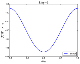
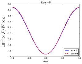
(i) (ii)

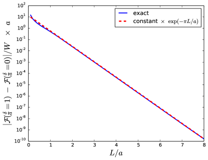
Figure 10: (i) Free energy per unit length (measured in units of $a$), as given by the exact formula of Eq. (46), as a function of $\delta$, for different values of $L$. The left curve ($L/a=0.1$) is well approximated by the asymptotic formula of Eq. (48) valid for $L\ll a$, while the right curve ($L/a=8$) is well approximated by $\cos(\pi\frac{\delta}{a})$ times an $L$-dependent amplitude. For the latter case, we have rescaled the free energy and subtracted a constant offset. (ii) The amplitude of the periodic modulation, defined as $\frac{1}{W}|\mathcal{F}(\frac{\delta}{a}=1)-\mathcal{F}(\frac{\delta}{a}=0)|$, decays as $e^{-\pi\frac{L}{a}}$ at large $L$.

To study the Casimir interaction at arbitrary separations, we have evaluated the free energy from the (modified) Szegö formula of Eq. (46) by numerical summation of the series and integration over $\theta$. In addition, we have obtained the free energy directly from a numerical computation of the determinant of truncated versions of the infinite matrix $G_{I}$ [see Eq. (42a)] and extrapolation of the results to $N\to\infty$. Both methods yield coincident results. The free energy per unit length is shown in Fig. 9 as function of the rescaled separation $L/a$ for different values of the lateral shift $\delta$. As expected from the limiting behavior of the free energy and small and large separations $L$, the free energy shows a minimum if $a>\delta>a/24$. This minimum is most pronounced for $\delta$ slightly larger than $a/24$, and for larger $\delta$ becomes more shallow and displaced to larger $L/a$. Hence, be tuning the lateral shift of the boundaries, different equilibrium positions of the boundaries can be achieved.

In order to study the lateral variation of the Casimir interation, we have also computed the free energy per unit length for three different fixed separations ($L/a=0.1,\,1.0,\,8.0$) as function of the lateral shift over one period ($-a\leq\delta\leq a$), see Fig. 10(i). At short separations, $L/a=0.1$, we recover the approximation of Eq. (48) with good accuracy. Towards intermediate distances, $L/a=1$, the dependence on $\delta$ becomes more cosine like and finally at sufficiently large separations $L/a=8$, we find convergence to a perfect $\cos(\pi\delta/a)$ dependence on $\delta$. This simple cosine dependence of the Casimir force has been observed before for QED Casimir forces between geometrically structured surfaces at large separations, irrespective of the precise form of the surface’s periodic pattern Büscher and Emig (2005). Similarly, for the Ising strip (and other CFT models) we expect for more complicated but periodic spin boundary conditions a convergence to such a simple cosine dependence at large separations. This follows from the fact that the free energy must be a periodic function of $\delta$ and hence can be decomposed into a discrete Fourier series. As we shall see in a moment, the amplitudes of the harmonics decay exponentially with $2\pi L/\lambda$ where $\lambda=2a/m$ is the wavelength of the harmonic function of order $m$. Hence, higher harmonics with $m>1$ are more strongly suppressed at large $L$, leaving only a cosine dependence from $m=1$. The dependence of the free energy on $\delta$ yields a lateral Casimir force $F_{\text{lat}}=-\partial\mathcal{F}/\partial\delta$ that is determined by the curves in Fig. 10(i).

Fig. 10(ii) shows the dependence of the amplitude of the modulation of the free energy with $\delta$, and hence the decay of the lateral force $F_{\text{lat}}$ with $L$. For sufficiently large $L/a$ the amplitude and hence the lateral force decays exponentially as $\sim e^{-\pi L/a}$ which is in agreement with the decay expected for the lowest harmonic with $m=1$.

V.2 Ising model with periodically alternating boundary conditions on one side

Figure 11: Configuration II: Ising model on an infinite strip with periodically alternating boundary conditions on one side, and homogeneous boundary conditions on the other side. On the upper boundary, the number of up spins (over length $a$) and down spins (over length $b$) can be different.

Now we focus on the configuration II (see Sec. III), and we show in detail how to recover the results of Eqs. (19) and (21) from the analysis of the asymptotics of a block-Toeplitz determinant. Notice that the total length of the strip is now $W=N(a+b)$ in Eq. (38), and the free energy per unit length is then, for $N\rightarrow+\infty$,

$$\frac{{\cal F}_{\text{CFT}}}{W}=-\frac{\pi}{48L}-\lim_{N\to\infty}\frac{1}{2N(a+b)}\log\left|\det G_{\text{II}}\right|\,.$$ (51)

The block-Toeplitz matrix $G_{\text{II}}$ whose determinant we need to evaluate is defined by the following blocks,

$$(p\neq 0)\qquad g_{p}=\left(\begin{array}[]{cc}\left<\psi(w_{2j})\psi(w_{2j+2p})\right>&\left<\psi(w_{2j})\psi(w_{2j+2p+1})\right>\\ \left<\psi(w_{2j+1})\psi(w_{2j+2p})\right>&\left<\psi(w_{2j+1})\psi(w_{2j+2p+1})\right>\end{array}\right)=\left(\begin{array}[]{cc}\frac{1}{\frac{2L}{\pi}\sinh\frac{\pi(a+b)p}{2L}}&\frac{1}{\frac{2L}{\pi}\sinh\frac{\pi(a+b)p+\pi a}{2L}}\\ \frac{1}{\frac{2L}{\pi}\sinh\frac{\pi(a+b)p-\pi a}{2L}}&\frac{1}{\frac{2L}{\pi}\sinh\frac{\pi(a+b)p}{2L}}\end{array}\right),$$ (52a)

$$g_{0}=\left(\begin{array}[]{cc}0&\left<\psi(w_{2j})\psi(w_{2j+1})\right>\\ \left<\psi(w_{2j+1})\psi(w_{2j})\right>&0\end{array}\right)=\left(\begin{array}[]{cc}0&\frac{1}{\frac{2L}{\pi}\sinh\frac{\pi a}{2L}}\\ -\frac{1}{\frac{2L}{\pi}\sinh\frac{\pi a}{2L}}&0\end{array}\right).$$ (52b)

A brief account of our results for this configuration has been given in Ref. Dubail et al. (2016). Below we shall give further details on the derivation of the results.

V.2.1 Asymptotics for small separations $L\ll a,b$

In the regime of a narrow strip, $L\ll a,b$, we can approximate $\sinh\frac{\pi(a+b)p}{2L}$ by $\frac{1}{2}e^{\frac{\pi(a+b)p}{2L}}$, and write similar expressions for the other entries of the blocks in Eq. (52). Again, this case is exactly equivalent to the one we treated in Sec. IV.2 [see Eq. (33)] now with $u=e^{-\frac{\pi a}{2L}}$ and $v=e^{-\frac{\pi b}{2L}}$. We saw in Eq. (32) that the determinant is always $u^{2n}=e^{-n\frac{\pi a}{L}}$. Thus, we recover the result of Eq. (19),

$$\frac{\mathcal{F}_{\text{CFT}}}{W}=-\frac{\pi}{48L}+\frac{\pi}{2L}\frac{a}{a+b}+\ldots\,,$$ (53)

where we have ignored again subleading logarithmic corrections.

V.2.2 Asymptotics for large separations $L\gg a,b$

The symbol of the block-Toeplitz matrix of Eq. (52) is

$$\varphi_{II}(\theta)=\frac{\pi}{L}\left(\begin{array}[]{cc}i\gamma^{II}_{1}(\theta)&-(\gamma^{II}_{2}(\theta))^{*}\\ \gamma^{II}_{2}(\theta)&i\gamma^{II}_{1}(\theta)\end{array}\right),\qquad\gamma^{II}_{1}(\theta)=\sum_{p=1}^{\infty}\frac{\sin(p\theta)}{\sinh\frac{\pi p(a+b)}{2L}}\,,\qquad\gamma^{II}_{2}(\theta)=\frac{1}{2}\sum_{p\in\mathbb{Z}}\frac{e^{ip\theta}}{\sinh\frac{\pi(p(a+b)-a)}{2L}}\,.$$ (54)

One can check that the index $\mathcal{I}_{2}$ is

$$\mathcal{I}_{2}={\rm sign}[b-a].$$ (55)

When $L\gg a,b$, the asymptotics of the functions $\gamma_{1}^{II}(\theta)$ and $\gamma_{2}^{II}(\theta)$ can be read directly from the formulas (93), (99) and (111) with the substitutions $\beta\rightarrow\pi(a+b)/(2L)$ and $\alpha\rightarrow\pi a/(2L)$, yielding

$$\gamma^{II}_{1}(\theta) = \frac{L}{a+b}\left\{\hat{\gamma}_{1}(\theta)+\tanh\left(\frac{L\theta}{a+b}\right)+\tanh\left(\frac{L(\theta-2\pi)}{a+b}\right)\right\}$$ (56a)

$$\gamma^{II}_{2}(\theta) = \frac{L}{a+b}\left\{\hat{\gamma}_{2}(\theta,\tau)+i\left[\tanh\left(\frac{L\theta}{a+b}\right)+\tanh\left(\frac{L(\theta-2\pi)}{a+b}\right)\right]\right\}$$ (56b)

with

$$\hat{\gamma}_{1}(\theta) = 1-\frac{\theta}{\pi}\,,$$

$$\hat{\gamma}_{2}(\theta,\tau) = \frac{1}{\pi}\left[-\frac{\tau+2}{\tau+1}+e^{i\theta}(\tau+2){}_{2}F_{1}\left(1,\frac{1}{\tau+2};\frac{\tau+3}{\tau+2};e^{i\theta}\right)-e^{-i\theta}\frac{\tau+2}{2\tau+3}{}_{2}F_{1}\left(1,\frac{2\tau+3}{\tau+2};\frac{3\tau+5}{\tau+2};e^{-i\theta}\right)\right].\quad$$ (57)

We recall that the parameter $\tau$ was defined as $\tau=a/b-1$ in Eq. (24). In the following we treat the cases $a<b$ and $a>b$ separately since they differ in the index $\mathcal{I}_{2}$ and hence require the application of different versions of the Szegö limit formula.

The case $a<b$ ($\mathcal{I}_{2}=+1$). Using the expressions (56a) and (56b), for $a<b$ (or $\tau<0$), Eq. (31) yields the free energy density per unit length

$$\frac{{\cal F}_{\text{CFT}}}{W}=-\frac{\pi}{48L}-\frac{1}{4\pi(a+b)}\int_{0}^{2\pi}d\theta\;\log\left\{1+\Gamma(\theta,\tau)\left[\tanh{\left(\frac{\theta L}{a+b}\right)}+\tanh{\left(\frac{(\theta-2\pi)L}{a+b}\right)}\right]\right\}\,,$$ (58)

where

$$\Gamma(\theta,\tau)=\frac{2\hat{\gamma}_{1}(\theta)+i(\hat{\gamma}_{2}(\theta,\tau)-\hat{\gamma}^{*}_{2}(\theta,\tau))}{|\hat{\gamma}_{1}(\theta)|^{2}-|\hat{\gamma}_{2}(\theta,\tau)|^{2}}.$$ (59)

To obtain Eq. (58) we have subtracted an a term that is $L$-independent and hence does not contribute to the Casimir force. Notice also that the $\log L$ term originating from the global factor $\pi/L$ of $\varphi_{II}(\theta)$, see Eq. (54), is cancelled by another one coming from the scaling with $L$ of $\gamma^{II}_{1}(\theta)$ and $\gamma^{II}_{2}(\theta)$, see Eqs. (56a) and (56b). We note that the rescaled free energy $L\mathcal{F}_{\rm CFT}$ depends only on $\tau$ and $(a+b)/L$.

Figure 12: Graph of the function $\Gamma(\theta,\tau)$, defined in Eq. (59), for different values of $\tau$.

The integrand in Eq. (58) is exponentially localized around $\theta=0,2\pi$ over a range $\sim(a+b)/L$. Therefore, it is important to consider the scaling behavior of the function $\Gamma(\theta,\tau)$ around $\theta=0$ and $\theta=2\pi$. This function is shown in Fig. (12) for different values of $\tau$. Expanding the numerator and the denominator of Eq. (59) around $\theta=0$ and $\tau=0$, the function $\Gamma(\theta,\tau)$ has the expansion

$$\Gamma(\theta,\tau)=\frac{\frac{2}{\pi}\theta}{\frac{\pi^{2}}{16}\tau^{2}+\frac{2}{\pi}\theta}+O\left(\theta^{2},\tau\theta,\tau^{3}\right),$$ (60)

that implies the following scaling behavior when $\tau\to 0$,

$$\Gamma\left(\zeta|\tau|^{x},\tau\right)\underset{\tau\rightarrow 0}{=}\begin{cases}1&\text{if $0<x<2$},\\ \frac{\zeta}{\zeta+\pi^{3}/32}&\text{if $x=2$},\\ 0&\text{if $x>2$},\end{cases}$$ (61)

for any constant $\zeta$. From this behavior of $\Gamma(\theta,\tau)$ it is evident that the relevant length scale to be compared to $L$ is $\xi_{c}(\tau)\sim(a+b)|\tau|^{-2}$ introduced in Eq. (24) and Eq. (25). It is crucial to realize that the two limits $L/(a+b)\to\infty$ and $\tau\to 0$ do not commute. Hence, we need to distinguish three different scaling regimes for $\tau\to 0$, depending on the value of $L/\xi_{c}$ that we shall identify with $1/\zeta$:

1. The regime $L\gg\xi_{c}$ or $L/(a+b)\sim\tau^{-x}$, $x>2$ (fixed spin BCs): The behavior of the integral in Eq. (58) depends on the limits of $\Gamma(\theta,\tau)$ when $\theta\to 0^{+}$ and $\theta\to 2\pi^{-}$, which are both zero so that the integral vanishes. The free energy per unit length is then to leading order $\mathcal{F}_{\rm CFT}/W=-\frac{\pi}{48L}$, which corresponds to like fixed spin boundary conditions on both sides, as argued in Eq. (21).

2. The regime $L\ll\xi_{c}$ or $L/(a+b)\sim\tau^{-x}$, $0<x<2$ (free-fixed spin BCs): The integral in Eq. (58) can be treated as follows. We consider first the part of integration from $0$ to $\pi$. We split the integration into two intervals, $0\leq\theta\leq C\tau^{x}$ and $C\tau^{x}\leq\theta\leq\pi$, for some fixed constant $C>0$. After a change of variables, $\theta\to\tilde{\theta}=L\theta/(a+b)$, the integral can be approximated by

   $$-\frac{1}{4\pi(a+b)}\int_{0}^{2\pi}d\theta\;\log\left\{1+\Gamma(\theta,\tau)\left[\tanh{\left(\frac{\theta L}{a+b}\right)}+\tanh{\left(\frac{(\theta-2\pi)L}{a+b}\right)}\right]\right\}$$

   $$\qquad\simeq-\frac{1}{4\pi L}\int_{CL\tau^{x}/(a+b))}^{\infty}\log\left\{1+\Gamma\left(\frac{(a+b)\tilde{\theta}}{L},\tau\right)\left[\tanh{\tilde{\theta}}-1\right]\right\}\;d\tilde{\theta}$$

   $$\qquad\qquad-\frac{1}{4\pi L}\int_{0}^{CL\tau^{x}/(a+b))}\log\left\{1+\Gamma\left(\frac{(a+b)\tilde{\theta}}{L},\tau\right)\left[\tanh{\tilde{\theta}}-1\right]\right\}\;d\tilde{\theta}.$$

   Because of the factor $\tanh\tilde{\theta}-1$, the first integral is localized around $CL\tau^{x}/(a+b)$ while the second term is of order $CL\tau^{x}/(a+b))$, since the integrand is bounded. Replacing $\Gamma$ by $1$, see Eq. (61), and taking the limit $C\to 0$, we see that the second integral vanishes, while the first one becomes

   $$-\frac{1}{4\pi L}\int_{0}^{\infty}\;d\tilde{\theta}\log\left[\tanh{(\tilde{\theta})}\right]=\frac{\pi}{32L}.$$

   The same contribution comes from the integration from $\pi$ to $2\pi$ in Eq.  (58). Hence, the free energy $\mathcal{F}_{\rm CFT}/W=-\frac{\pi}{48L}+\frac{\pi}{16L}=\frac{\pi}{24L}$, as expected from Eq. (21) for a strip with free spin BCs on one and fixed spin BCs on the other side.

3. The scaling regime $L\sim\xi_{c}$ or $L/(a+b)\sim\tau^{-2}$ (flow from free spin BCs to fixed spin BCs): this is probably the most interesting case since it yields the scaling function that describes the flow from free to fixed boundary conditions. To evaluate the integral in Eq. (58), one proceeds again by splitting the integral into two parts, exactly as in the previous case. Replacing $\Gamma(\zeta\tau^{2},\tau)$ by $\zeta/(\zeta+\pi^{2}/32)$, see Eq. (61), we find the following expression for the free energy per unit length,

   $$\frac{\mathcal{F}_{\text{CFT}}}{W} = -\frac{\pi}{48}\frac{1}{L}-\frac{1}{L}\frac{1}{2\pi}\int_{0}^{\infty}\;d\tilde{\theta}\log\left\{1+\frac{\zeta}{\zeta+\pi^{2}/32}(\tanh{(\tilde{\theta})}-1)\right\}$$ (62)

   $$= \frac{1}{4\pi L}\text{Li}_{2}\left(\frac{2\zeta}{\zeta+\pi^{3}/32}-1\right),$$

   where $\text{Li}_{2}(x)$ is the polylogarithm function. Hence, identifying the scaling variable $\zeta$ with $\xi_{c}/L$, we conclude that the exponent $\nu_{c}$ defined in Eq. (25) is indeed $2$ and the free energy takes the form

   $$\frac{\mathcal{F}_{\text{CFT}}}{W}=\frac{\vartheta_{-}(\zeta)}{L},$$ (63)

   where the universal scaling function $\vartheta_{-}(\zeta)$ for $a<b$ is given by

   $$\vartheta_{-}(\zeta)=\frac{1}{4\pi}\text{Li}_{2}\left(\frac{2\zeta}{\zeta+\pi^{3}/32}-1\right)\,.$$ (64)

The case $a>b$ ($\mathcal{I}_{2}=-1$). In this case the large $N$ asymptotic of the Toeplitz determinant is given by Eq. (36b). Note that the contribution to the free energy coming from the term $\int_{0}^{\pi}\frac{d\theta}{2\pi}\log\det\varphi_{II}(\theta)\;$ is symmetric in $a$ and $b$ and is still given by the Eq. (58). Analogously to the case of configuration $I$ with $\delta>a/2$, see Eq. (46) and Eq. (47), we have to add to Eq. (58) the decay rate $\kappa$:

$$\kappa=-\lim_{n\to\infty}\frac{1}{n}\log\det\int_{0}^{2\pi}\frac{d\theta}{2\pi}e^{in\theta}\varphi^{-1}_{II}(\theta)\,.$$ (65)

The free energy per unit length is therefore

$$\frac{\mathcal{F}_{\text{CFT}}}{W}=\text{r.h.s. of Eq.~{}\eqref{Eq:Free_energy_II_largeL}}+\frac{\kappa}{(a+b)}\,.$$ (66)

We recall that $\kappa$ is determined by the location of the nearest pole $\theta_{s}$ to the real axis of the function $[\varphi_{II}^{-1}(\theta)]_{11}$. The pole $\theta_{s}$ is obtained from the zeros of the determinant, $\det\varphi_{II}(\theta_{s})=0$. In particular one has $\kappa=\Im(\theta_{s})$. To determine $\kappa$, we can use the expansions of Eqs. (91) and (108) with $\beta=\pi(a+b)/2L$ and $\tilde{\epsilon}\sim\tau/2$, where $\tau$ is defined in Eq. (24). We find that

$$\text{det}\;\varphi_{II}(\theta)=\frac{\pi^{4}}{64}\tau^{2}+\frac{\pi}{2}\theta\;\tanh\left(\frac{L\theta}{a+b}\right)+O\left(\frac{\tau}{L}\right)$$ (67)

The value of $\kappa$ is therefore given by the solution of the non-linear equation

$$\frac{\pi^{4}}{64}\tau^{2}-\frac{\pi}{2}\kappa\tan\left(\frac{L\kappa}{a+b}\right)=0\,.$$ (68)

As shown in Fig. (13), the solutions of Eq. (68) depend on the following three scaling regimes for $\tau\to 0$:

1. The regime $L\gg\xi_{c}$ or $L/(a+b)\sim\tau^{-x}$, $x>2$ (fixed -, fixed + spin BCs). In this regime, the Eq. (68) yields

   $$\kappa=\pi\frac{a}{L}+O(L^{2\frac{1-x}{x}})$$ (69)

   The free energy Eq. (66) then becomes $\mathcal{F}_{\text{CFT}}/W=-\frac{\pi}{48L}+\frac{\kappa}{(a+b)}=-\frac{\pi}{48L}+\frac{\pi}{2L}=+\frac{\pi}{L}\frac{23}{48}$ and we recover the $(-,+)$ BCs of Eq. (21).

2. The regime $L\ll\xi_{c}$ or $L/(a+b)\sim\tau^{-x}$, $0<x<2$ (free-fixed spin BCs). In this regime, the solution of Eq. (68) takes the form

   $$\kappa\sim L^{-\frac{2+x}{2x}}\,.$$ (70)

   The free energy Eq. (66) is still given by $\mathcal{F}_{\text{CFT}}/W=-\frac{\pi}{48L}+\frac{\pi}{16L}$ as $\kappa$ gives a sub-leading contribution, $\kappa\sim O(L^{-1})$. Hence we recover thus the result Eq.(21) for $(f,+)$ BCs.

3. The scaling regime $L\sim\xi_{c}$ or $L/(a+b)\sim\tau^{-2}$ (flow from the free to fixed + spin BCs). We can write the non-linear equation for $\kappa$ in terms of the scaling variable $\zeta$ with $L/(a+b)=\zeta\tau^{-2}$ in the compact form

   $$\Delta\vartheta(\zeta)\tan\left[\Delta\vartheta(\zeta)\right]=\frac{\pi^{3}}{32}\zeta,$$ (71)

   where we defined

   $$\frac{\Delta\vartheta}{L}=\frac{\kappa}{(a+b)}\,.$$ (72)

   Using Eqs. (64) and (66), the universal scaling function $\vartheta_{+}(\zeta)$, defined by

   $$\frac{\mathcal{F}_{\text{CFT}}}{W}=\frac{\vartheta_{+}(\zeta)}{L}$$ (73)

   is given by

   $$\vartheta_{+}(\zeta)=\vartheta_{-}(\zeta)+\Delta\vartheta(\zeta)\,.$$ (74)

Figure 13: The panels show, from the left to the right, the solution of the Eq. (68) in the three regimes (i), (ii) and (iii) discussed in the text. In particular, the values of the exponent $x$, $L/(a+b)\sim\tau^{-x}$ have been set to $x=(5,3/2,2)$ for the regime (i), (ii) and (iii) respectively. The parameters $a$ and $b$ have been chosen such that $a+b=1$.

V.2.3 Arbitrary separations $L$

To study the free energy for arbitrary separations, and to determine the position of the energy minimum for the cases with $b/23<a<b$, we have evaluated Eq. (51) numerically for different ratios $a/b$, following the procedure outline above for configuration I.The result is shown in Fig. 14. The minimum in the free energy is most pronounced for $a/b$ slightly larger than $1/23$. For increasing values of $a/b$ the minimum becomes rather shallow.

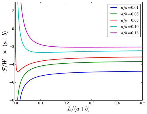
Figure 14: Free energy per unit length (measured in units of $a+b$), as given by the exact formula of Eq. (51) as function of $L$ for different values of $a/b$. Note that the free energy shown here contains ($L$-independent) surface self-energies and hence does not vanish for $L\to\infty$. The self-energies depend on the boundary conditions and hence on $a/b$.

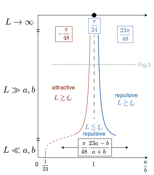
Figure 15: Schematic overview of critical Casimir force amplitudes as function of the strip width $L$ and the ratio $a/b$. For $L\gg a,b$ the solid curves represent the diverging crossover length $\xi_{c}$. The horizontal dashed line indicates the cut along which the force amplitude is plotted in Fig. 16. Across the red curve the sign of the force changes whereas the blue curve indicates only a change between two universal (repulsive) limits.

Figure 16: Universal scaling function $\Theta(x_{s})$ for the critical Casimir force as function of the scaling variable $x_{s}\sim a-b$.

Our overall findings for configuration II can be summarized by the scheme of Fig. 15. It shows the different scaling regimes and the corresponding asymptotic amplitudes of the Casimir force. At short distance $L\ll a,b$ the amplitude varies continuously across the critical point at $a=b$, with a sign change at $b/a=23$. For $L\gg a,b$ there exist three distinct regions: around $a=b$ appears a region where $L\ll\xi_{c}$ where the force is repulsive and approaches for asymptotic $L$ the universal amplitude for fixed-free spin boundary conditions. For $a<b$, the force changes sign from attractive to repulsive when $L$ approaches $\xi_{c}$, corresponding to a stable point. For $a>b$, the force is always repulsive but the amplitude crosses over from $\pi/24$ to $23\pi/48$ under an increase of $L$ beyond $\xi_{c}$.

The dependence of the force $F$ on $|a-b|$ at fixed $L\gg a,b$ (see dashed horizontal line in Fig. 15) is determined by $F=-\partial{\cal F}/\partial L=\Theta(x_{s})L^{-2}$ with a universal scaling function $\Theta$ of the scaling variable $x_{s}$ that is defined on both sides of the critical point by $x_{s}=\text{sign}(\tau)(L/\xi_{c})^{1/2}\sim a-b$. This function is shown in Fig. 16 where we used the results for $\vartheta_{\pm}(\zeta)$ of Eqs. (64), (74). In the critical region $|x_{s}|\ll 1$, one has the expansions

$$\Theta(x_{s})=\left\{\begin{array}[]{ll}\frac{\pi}{24}-\frac{\pi^{2}}{64}x_{s}^{2}+\ldots&\text{for }x_{s}<0\\[10.00002pt] \frac{\pi}{24}+\frac{\pi^{3/2}}{8\sqrt{2}}x_{s}+\ldots&\text{for }x_{s}>0\end{array}\right.\,,$$ (75)

whereas for $L$ outside the critical region, $|x_{s}|\gg 1$,

$$\Theta(x_{s})=\left\{\!\begin{array}[]{ll}-\frac{\pi}{48}+\frac{32\log 2}{\pi^{4}}\frac{1}{x_{s}^{2}}+\ldots&\text{for }x_{s}<0\\[10.00002pt] \frac{23\pi}{48}-\frac{32(\pi^{2}-\log 2)}{\pi^{4}}\frac{1}{x_{s}^{2}}+\ldots&\text{for }x_{s}>0\end{array}\right..$$ (76)

We see that $\Theta(x_{s})$ is not analytic around $x_{s}=0$ and hence constitutes a singular part of the free energy density. This resembles the singular nature of scaling functions describing the bulk transition at $T=T_{c}$.

VI Conclusion

We have demonstrated that boundary CFT is a powerfull tool to study critical Casimir forces in two dimensional systems with inhomogeneous boundary conditions. We have studied explicitly a Ising strip at its critical temperature with periodically varying boundary conditions along the edges of the strip. Depending on the relative number and position of the fixed spins at the edges, we have observed a number of interesting phenomena:

1. At short separation between the edges, their Casimir interaction is determined by additivity, i.e., by a superposition of the interaction for like and unlike fixed spin boundary conditions.

2. If an edge has identical numbers of fixed up and down spins, at large separations it contributes to the Casimir interaction effectively as an edge with homogeneous free spin boundary conditions.

3. When the fixed spin boundary conditions break $\mathbb{Z}_{2}$ symmetry (edge with unequal number of up and down spins) the effective boundary condition determining the Casimir force depends on the edge separation. The crossover in the Casimir interaction between the different boundary conditions is described by a universal scaling function.

4. The normal Casimir force between the edges can be attractive or repulsive. There are cases where the force changes sign from attractive to repulsive when the edge separation is reduced, leading to a stable equilibrium position.

5. For the configurations studied here, a stable position (with respect to the normal separation $L$) exists for configuration I if the lateral shift $\delta$ obeys the condition $a/24<|\delta|<a$ (modulo periodicity) and for configuration II if the modulation length obey the condition $b/23<a<b$.

6. When both edges have periodically modulated fixed spin boundary conditions, there acts a lateral Casimir force between them. This force decays exponentially with the edge separation over a length scale that is given by the wavelength of the boundary conditions. At short separations, the lateral force follows from additivity, leading to a piecewise constant force. At large separations, the lateral force assumes a universal form that follows a simple cosine profile.

The observed renormalization of modulated fixed spin boundary conditions, in binary mixtures, allows for an experimental realization of ordinary (free spin) boundary conditions. These boundary conditions can be “switched” on and off by varying the distance $L$, or an inhomogeneous surface field. The position of the minimum of the free energy can be tuned either by varying the lateral shift between the boundaries or by changing the relative number of up and down spins. This provides external control parameters to define a preferred equilibrium separation between the surfaces. It is interesting to explore these concepts in three dimensions for Ising and XY models, and tri-critical points which have an even richer spectrum of possible boundary conditions. Previous mean field and numerical studies of a 3D Ising system confined between parallel boundaries with alternating boundary conditions indicated indeed the possibility of a sign change of the force Toldin et al. (2013).

Acknowledgements. We are grateful to Davide Vodola, Jean-Marie Stéphan, Eddy Ardonne, Estelle Basor and Karol Kozlowski for very helpful discussions and exchange about section IV. We also thank Andrea Gambassi and Mehran Kardar for general discussions. This work was partially supported (JD) by the Conseil Général de Lorraine and the Université de Lorraine and by the CNRS ”Défi Inphyniti”. JD thanks Nordita, Stockholm, for hospitality during the workshop ”From quantum field theories to numerical methods”, where part of this work was done.

Appendix A Asymptotics infinite sums

We define the functions:

$$f_{1}(x)=\frac{\sin(x\theta)}{\sinh(\beta x)},\quad f^{\pm}_{2}(x)=\frac{\exp(\pm ix\theta)}{\sinh(\beta x\mp\alpha),}\quad f^{\pm}_{3}(x)=\frac{\exp(\pm ix\theta)}{\cosh(\beta x\mp\alpha)}$$ (77)

and the corresponding sums:

$$\gamma_{1}(\theta)=\sum_{n\in\mathbb{Z}^{+}}^{\infty}f_{1}(n),\quad\gamma_{2}(\theta)=\sum_{n\in\mathbb{Z}}^{\infty}f^{+}_{2}(n)\quad\text{and}\quad\gamma_{3}(\theta)=\sum_{n\in\mathbb{Z}}^{\infty}f^{+}_{3}(n).$$ (78)

We are interested in the asymptotics of the above sums in the limit:

$$\beta\to 0,\quad\alpha\to 0,\quad\text{and}\quad\frac{\alpha}{\beta}\to\text{constant}.$$ (79)

Unless otherwise stated, the variable $\theta$ runs in the interval $-\pi<\theta\leq\pi$.

We use the Euler-MacLaurin summation formula:

$$\sum_{n=n_{\text{min}}}^{\infty}f(x)=\int_{n_{\text{min}}}^{\infty}dxf(x)+\frac{1}{2}f(n_{\text{min}})+\Delta.$$ (80)

The rest term $\Delta$ in the above formula is given by:

$$\Delta=-\sum_{l=1}^{\infty}\frac{B_{2l}}{2l!}f^{(2l-1)}(n_{\text{min}}),$$ (81)

where the $B_{2l}$ are the Bernoulli numbers. We will also use the Abel-Plana formulation Dowling (1989) for the sum (80) with $n_{min}=0$. In Abel-Plana formula the rest $\Delta$ is expressed as:

$$\Delta=i\int_{0}^{\infty}\frac{f(iy)-f(-iy)}{e^{2\pi y}-1}.$$ (82)

A.1 Asymptotics of $\gamma_{1}(\theta)$

From the Eq. (80) and Eq. (81)) one obtains:

$$\gamma_{1}(\theta)=\int_{1}^{\infty}dxf_{1}(x)+\frac{\sin(\theta)}{2\sinh(\beta)}-\sum_{l=1}^{\infty}\frac{B_{2l}}{2l!}f_{1}^{(2l-1)}(1).$$ (83)

The above expression can be rewritten in the form:

$$\gamma_{1}(\theta)=\frac{1}{\beta}\left(\int_{0}^{\infty}dx-\int_{0}^{\beta}dx\right)\frac{\sin(x\theta/\beta)}{\sinh(x)}+\frac{\sin(\theta)}{2\sinh(\beta)}-\sum_{l=1}^{\infty}\frac{B_{2l}}{2l!}f_{1}^{(2l-1)}(1).$$ (84)

In the limit $\beta\to 0$ we can use the expansion $\sinh{\beta n}=\beta n+O(\beta^{2})$: the dominant contribution $\Delta^{0}_{1}$ in the expansion of the rest term:

$$\sum_{l=1}^{\infty}\frac{B_{2l}}{2l!}f_{1}^{(2l-1)}(1)=-\beta^{-1}\Delta^{0}_{1}+O(\beta^{0}),$$ (85)

is given by:

$$\Delta^{0}_{1}=-\sum_{l=1}^{\infty}\frac{B_{2l}}{2l!}\frac{d^{2l-1}}{dx^{2l-1}}\left[\frac{\sin{(x\theta)}}{x}\right](1)$$ (86)

The integrals:

$$\int_{0}^{\infty}dx\;\frac{\sin(xy)}{\sinh(x)}=\frac{\pi}{2}\tanh{\left(\frac{\pi}{2}y\right)},\quad\text{Si}(\theta)\equiv\int_{0}^{1}\;dx\frac{\sin{(\theta)x}}{x},$$ (87)

give, for the expansion (83), the following result:

$$\gamma_{1}(\theta)=\frac{1}{\beta}\left[\frac{\pi}{2}\tanh{\left(\frac{\pi\theta}{2\beta}\right)}+\frac{\sin(\theta)}{2}-\text{Si}(\theta)+\Delta_{1}^{0}\right]+O(\beta^{0}).$$ (88)

The term $\Delta_{1}^{0}$ in (86) can also be computed by applying the Euler-Maclaurin formula to the sum:

$$\sum_{n=1}^{\infty}\frac{\sin{\left(n\theta\right)}}{n}=\begin{cases}\frac{\pi}{2}-\frac{\theta}{2},&\text{if }\;0<\theta\leq\pi\\ -\frac{\pi}{2}-\frac{\theta}{2},&\text{if}\;\pi\leq\theta<0\\ 0&\text{if}\;\theta=0,\end{cases}.$$ (89)

One obtains:

$$\Delta_{1}^{0}=\frac{\theta}{2}-\frac{\sin(\theta)}{2}+\text{Si}(\theta).$$ (90)

Collecting all the previous formula one finally gets:

$$\gamma_{1}(\theta)=\frac{1}{\beta}\left(\frac{\pi}{2}\tanh{\left(\frac{\pi\theta}{2\beta}\right)}-\frac{\theta}{2}\right)+O(\beta^{0}),\quad\text{for}\;-\pi<\theta\leq\pi$$ (91)

The validity of (91) is verified in Fig (17).

Figure 17: The plots compare, for different values of $\beta=5,2,0.5$, the function $\gamma_{1}(\theta)$ computed using the sum in (78) and the asymptotic formula (91)

In the interval $0\leq\theta<2\pi$, the result (91) reads:

$$\gamma_{1}(\theta)=\begin{cases}\frac{1}{\beta}\left(\frac{\pi}{2}\tanh{\left(\frac{\pi\theta}{2\beta}\right)}-\frac{\theta}{2}\right),&\text{if }\;0\leq\theta\leq\pi\\ \frac{1}{\beta}\left(\frac{\pi}{2}\tanh{\left(\frac{\pi(\theta-2\pi)}{2\beta}\right)}-\frac{\theta}{2}+\pi\right).&\text{if}\;\pi<\theta<2\pi\end{cases}+O(\beta^{0}).$$ (92)

The above formuala can be approximated (with a difference $\sim e^{-1/\beta}$) by the expression:

$$\gamma_{1}(\theta)=\frac{1}{\beta}\left(\frac{\pi}{2}-\frac{\theta}{2}+\frac{\pi}{2}\tanh{\left(\frac{\pi\theta}{2\beta}\right)}+\frac{\pi}{2}\tanh{\left(\frac{\pi(\theta-2\pi)}{2\beta}\right)}\right)+O(\beta^{0})$$ (93)

A.2 Asymptotics of $\gamma_{2}(\theta)$

Using the identity:

$$\sum_{n\in\mathbb{Z}^{+}}\frac{e^{in\theta}}{\sinh{(\beta n-\alpha)}}=e^{i\theta+\alpha}\sum_{p=0}^{\infty}\frac{e^{2\alpha p}}{e^{\beta(2p+1)}-e^{i\theta}},$$ (94)

the sum $\gamma_{2}(\theta)$ can be written in the form:

$$\gamma_{2}(\theta)=-\frac{1}{2\sinh{(\alpha)}}+e^{i\theta+\alpha}\sum_{p=0}^{\infty}\frac{e^{2\alpha p}}{e^{\beta(2p+1)}-e^{i\theta}}-e^{-i\theta-\alpha}\sum_{p=0}^{\infty}\frac{e^{-2\alpha p}}{e^{\beta(2p+1)-e^{-i\theta}}}$$ (95)

Applying the summation formula (80) to the (94) and using the integral representation of the hypergeometric functions ${}_{2}F_{1}(a,b;c;z)$, we obtain:

$$\gamma_{2}(\theta) = -\frac{1}{2\sinh{(\alpha)}}+e^{\alpha+i\theta}\left[\frac{e^{-\beta}}{2(\beta-\alpha)}\,_{2}F_{1}\left(1,1-\frac{\alpha}{\beta};2-\frac{\alpha}{\beta};e^{i\theta-\beta}\right)+\frac{1}{2(e^{\beta}-e^{i\theta})}\right]-$$ (96)

$$-e^{-\alpha-i\theta}\left[\frac{e^{-\beta}}{2(\beta+\alpha)}\,_{2}F_{1}\left(1,\frac{\alpha}{\beta}+1;\frac{\alpha}{\beta}+2;e^{-\beta-i\theta}\right)+\frac{1}{2(e^{\beta}-e^{-i\theta})}\right]+\Delta_{2},$$

where a convenient expression for the rest $\Delta_{2}$ is found by the formula (82):

$$\Delta_{2}=i\int_{0}^{\infty}dy\frac{h^{+}(iy)-h^{-}(iy)-h^{+}(-iy)+h^{-}(-iy)}{e^{2\pi y}-1},\quad h^{\pm}(x)=\frac{e^{\pm 2\alpha x}}{e^{\beta(1+2x)-e^{\pm i\theta}}}.$$ (97)

A.2.1 $\beta,\alpha\to 0$ and $\theta>>\alpha,\beta$

In the limit $\beta,\alpha\to 0$ and $\theta>>\alpha,\beta$, it is straightforward to obtain from the above expression that:

$$\gamma_{2}(\theta)=\beta^{-1}\hat{\gamma}_{2}(\theta)+O(\alpha^{0},\beta^{0}),$$ (98)

where

$$\hat{\gamma}_{2}(\theta)=-\frac{\beta}{2\alpha}+e^{i\theta}\left[\frac{\beta}{2(\beta-\alpha)}\,_{2}F_{1}\left(1,1-\frac{\alpha}{\beta};2-\frac{\alpha}{\beta};e^{i\theta}\right)\right]-e^{-i\theta}\left[\frac{\beta}{2(\beta+\alpha)}\,_{2}F_{1}\left(1,\frac{\alpha}{\beta}+1;\frac{\alpha}{\beta}+2;e^{-i\theta}\right)\right].$$ (99)

The above expression expresses the leading behavior of $\gamma_{2}(\theta)$ for values of $\theta>>\alpha,\beta$. More subtle is to find the contribution to the leading term of $\gamma_{2}(\theta)$ coming from the region $\theta\leq\alpha,\beta$. In order to derive this contribution, we computed the small $\theta$ expansion of $\gamma_{2}(\theta)$.

A.2.2 $\beta,\alpha\to 0$ and $\theta<<\beta,\alpha$

Differently from what seen before, we use the summation formula (80) and (81) on the sum $\gamma_{2}(\theta)$ as expressed in (78):

$$\gamma_{2}(\theta)=\frac{1}{2}\left(\int_{2}^{\infty}dy\;f_{2}^{+}(x)-\int_{1}^{\infty}dy\;f_{2}^{-}(x)\right)+\frac{e^{i\theta}}{2\sinh{(\beta-\alpha)}}-\frac{1}{2\sinh{\alpha}}+\Delta_{2},$$ (100)

where the rest $\Delta_{2}$ is expressed now as:

$$\Delta_{2}=\sum_{l=1}^{\infty}\frac{B_{2l}}{(2l)!}\left(\frac{d^{(2l-1)}}{dx^{2l-1}}f^{-}_{2}(1)-\frac{d^{(2l-1)}}{dx^{2l-1}}f^{+}_{2}(2)\right).$$ (101)

It is convenient to express the functions under consideration in terms of the parameters $(\tilde{\theta},\beta,\tilde{\varepsilon})$ that are defined as:

$$\tilde{\epsilon}=2\frac{\alpha}{\beta}-1,\quad\tilde{\theta}=\frac{\theta}{\beta}.$$ (102)

The contribution coming from the integrals in (100) admits the following expansion in $\beta$ :

$$\frac{1}{2}\left(\int_{2}^{\infty}dy\;f_{2}^{+}(x)-\int_{1}^{\infty}dy\;f_{2}^{-}(x)\right)=\frac{e^{i\tilde{\theta}\beta(1-\tilde{\epsilon})/2}}{2\beta}\left(\int_{\beta(3/2-\tilde{\epsilon}/2)}^{\infty}\;dx\;\frac{e^{ix\tilde{\theta}}}{\sinh{(x)}}-\int_{\beta(3/2+\tilde{\epsilon}/2)}^{\infty}\;dx\;\frac{e^{-ix\tilde{\theta}}}{\sinh{(x)}}\right)=$$

$$=\beta^{-1}\left[-\text{coth}^{-1}\left(\frac{\tilde{\epsilon}}{3}\right)+i\frac{\pi}{2}\tanh\left(\frac{\pi\tilde{\theta}}{2}\right)-i\frac{\pi}{2}\right]+O(\beta^{0}).$$ (103)

The rest $\Delta_{2}$ behaves as:

$$\Delta_{2}=\beta^{-1}\Delta^{0}_{2}(\tilde{\epsilon})+O(\beta^{0},\tilde{\theta}),$$ (104)

where $\Delta^{0}_{2}(\tilde{\epsilon})$ is some function of $\tilde{\epsilon}$. We obtain therefore the following result:

$$\gamma_{2}(\tilde{\theta})=\beta^{-1}\left[-\text{coth}^{-1}\left(\frac{\tilde{\epsilon}}{3}\right)+i\frac{\pi}{2}\tanh\left(\frac{\pi\tilde{\theta}}{2}\right)-i\frac{\pi}{2}+\frac{1}{-1+\tilde{\epsilon}}+\frac{1}{1+\tilde{\epsilon}}+\Delta^{0}_{2}(\tilde{\epsilon})\right]+O(\beta^{0})$$ (105)

In the small $\tilde{\epsilon}$ expansion, the (105) yields:

$$\gamma_{2}(0)=\beta^{-1}\left[d_{0}+\tilde{\epsilon}\left(-\frac{7}{3}+d_{1}\right)+O(\tilde{\epsilon}^{2})\right]+O(\beta^{0}),$$ (106)

where $d_{0}$ and $d_{1}$ are the coefficients of the expansion of $\Delta^{0}_{2}(\tilde{\epsilon})=d_{0}+d_{1}\tilde{\epsilon}+O(\epsilon^{2})$. The direct computation of $\gamma_{2}(0)$:

$$\gamma_{2}(0) = \frac{1}{\beta}\sum_{n\geq 0}\left[\frac{1}{2n+(1+\tilde{\epsilon})}-\frac{1}{2n+(1-\tilde{\epsilon})}\right]+O(\beta^{0})=\beta^{-1}\left[-2\tilde{\epsilon}\sum_{n\geq 0}\frac{1}{(2n+1)^{2}}+O(\tilde{\epsilon})\right]+O(\beta^{0})=$$ (107)

$$= \beta^{-1}\left[-\frac{\pi^{2}}{4}\tilde{\epsilon}+O(\tilde{\epsilon}^{2})\right]+O(\beta^{0}),$$

fixes $d_{0}=0$ and $d_{1}=-\pi^{2}/4+7/3$.

We have obtained therefore the following expansion of $\gamma_{2}(\theta)$ for small $\tilde{\epsilon}$:

$$\gamma_{2}(\tilde{\theta})=\beta^{-1}\left[-\frac{\pi^{2}}{4}\tilde{\epsilon}+i\frac{\pi}{2}\tanh\left(\frac{\pi\tilde{\theta}}{2}\right)+O(\tilde{\epsilon}^{2})\right]+O(\beta^{0}).$$ (108)

Comparing the above result with the small $\tilde{\epsilon}$ expansion of $\hat{\gamma}_{2}(0)$ in (99):

$$\hat{\gamma}_{2}(0)=\begin{cases}-i\frac{\pi}{2}-\frac{\pi^{2}}{4}\tilde{\epsilon}+O(\tilde{\epsilon}^{2}),&\text{if }\;0\leq\theta\leq\pi\\ i\frac{\pi}{2}-\frac{\pi^{2}}{4}\tilde{\epsilon}+O(\tilde{\epsilon}^{2}),&\text{if}\;-\pi<\theta<0\end{cases},$$ (109)

we find:

$$\gamma_{2}(\theta)=\begin{cases}\beta^{-1}\left[\hat{\gamma}_{2}(\theta)+i\frac{\pi}{2}\left(\tanh\left(\frac{\pi\theta/\beta}{2}\right)-1\right)\right],&\text{if }\;0\leq\theta\leq\pi\\ \beta^{-1}\left[\hat{\gamma}_{2}(\theta)+i\frac{\pi}{2}\left(\tanh\left(\frac{\pi\theta/\beta}{2}\right)+1\right)\right].&\text{if}\;-\pi<\theta<0\end{cases}+O(\beta^{0}).$$ (110)

The above asymptotics are checked in Fig. (18).

Figure 18: The plots compare the real and imaginary part of the functions $\gamma_{2}(\theta)$ computed from (78) and its asymptotics (110) for values of $(\alpha,\beta)=(1,1.5),(0.1,0.15)$.

A compact expression in the interval $0\leq\theta<2\pi$ providing an approximation $\sim e^{-1/\beta}$ to the asymptotics (110) is:

$$\gamma_{2}(\theta)=\beta^{-1}\left[\hat{\gamma}_{2}(\theta)+i\frac{\pi}{2}\left(\tanh{\left(\frac{\pi\theta}{2\beta}\right)}+\tanh{\left(\frac{\pi(\theta-2\pi)}{2\beta}\right)}\right)\right]+O(\beta^{0})$$ (111)

A.3 Asymptotics of $\gamma_{3}(\theta)$

In the limit $\beta,\alpha\to 0$ and in the region $\theta>>\beta,\alpha$, one can replaces $\cosh(\beta n-\alpha)$ by one, as $\cosh(\beta n-\alpha)=1+O(\beta^{-2})$.

In this case one obtains:

$$\gamma_{3}(\theta)=0+O(\beta^{-2})\quad\theta>>\beta$$ (112)

In the region $\theta\leq\beta$, the asymptotics of the function $\gamma_{3}(\theta)$ can be found as in the previous case by using the formula (81):

$$\gamma_{3}(\theta)=\frac{1}{2}\left(\int_{2}^{\infty}dy\;f_{3}^{+}(x)+\int_{1}^{\infty}dy\;f_{3}^{-}(x)\right)+\frac{e^{i\theta}}{2\cosh{(\beta-\alpha)}}-\frac{1}{2\cosh{\alpha}}+\Delta_{3}$$ (113)

where

$$\Delta_{3}=\sum_{l=1}^{\infty}\frac{B_{2l}}{(2l)!}\left(\frac{d^{(2l-1)}}{dx^{2l-1}}f^{-}_{3}(1)-\frac{d^{(2l-1)}}{dx^{2l-1}}f^{+}_{3}(2)\right).$$ (114)

One can verify that the rest term $\Delta_{3}$ behaves as:

$$\Delta_{3}=i\left(e^{i\theta}-e^{2i\theta}\right)\frac{-2+\theta\cot(\theta/2)}{2x}+O(\beta^{2}),$$ (115)

thus producing a term of order $\beta^{0}$, $\Delta_{3}=O(1)$ The only terms that contribute with a $O(\beta^{-1})$ term are the integrals in (113). Using the same manipulations as before, one obtains:

$$\gamma_{3}(\theta)=\beta^{-1}\left[\frac{\pi}{2}e^{i\theta\frac{\alpha}{\beta}}\cosh\left(\frac{\pi\theta}{\beta 2}\right)^{-1}\right]+O(\beta^{0}).$$ (116)

The validity of the above asymptotic is tested in Fig. (19). In the interval $0\leq\theta<2\pi$ the (116) takes the form:

$$\gamma_{3}(\theta)=\begin{cases}\beta^{-1}\left[\frac{\pi}{2}e^{i\theta\frac{\alpha}{\beta}}\cosh\left(\frac{\pi\theta}{\beta 2}\right)^{-1}\right],&\text{if }\;0\leq\theta\leq\pi\\ \beta^{-1}\left[\frac{\pi}{2}e^{i(\theta-2\pi)\frac{\alpha}{\beta}}\cosh\left(\frac{\pi(\theta-2\pi)}{\beta 2}\right)^{-1}\right].&\text{if}\;-\pi<\theta<0\end{cases}+O(\beta^{0}).$$ (117)

Figure 19: The plots compares the real and imaginary part of the function $\gamma_{3}(\theta)$ as in (78) with its asymptotics (116)

References

• Parsegian (2005) V. A. Parsegian, Van der Waals Forces (Cambridge University Press, 2005).
• Casimir (1948) H. B. G. Casimir, Proc. K. Ned. Akad. Wet. 51, 793 (1948).
• Bordag et al. (2009) M. Bordag, G. L. Klimchitskaya, U. Mohideen, and V. M. Mostepanenko, Advances in the Casimir Effect (Oxford University Press, 2009).
• de Gennes and Fisher (1978) P.-G. de Gennes and M. E. Fisher, C. R. Acad. Sci. Ser. B 287, 207 (1978).
• Krech (1994) M. Krech, The Casimir effect in Critical systems (World Scientific, 1994).
• Gambassi (2009) A. Gambassi, J. Phys.: Conf. Ser. 161, 012037 (2009).
• Diehl (1986) H.-W. Diehl, Phase Transitions and Critical Phenomena (Academic Press, London, 1986), vol. 10, p. 75.
• Abraham and Maciolek (2010) D. B. Abraham and A. Maciolek, Phys. Rev. Lett. 105, 055701 (2010).
• Vasilyev et al. (2011) O. Vasilyev, A. Maciolek, and S. Dietrich, Phys. Rev. E 84, 041605 (2011).
• Munday et al. (2009) J. Munday, F. Capasso, and V. Parsegian, Nature 457, 170 (2009).
• Soyka et al. (2008) F. Soyka, O. Zvyagolskaya, C. Hertlein, L. Helden, and C. Bechinger, Phys. Rev. Lett. 101, 208301 (2008).
• Hertlein et al. (2008) C. Hertlein, L. Helden, A. Gambassi, S. Dietrich, and C. Bechinger, Nature 451, 172 (2008).
• Gambassi et al. (2009) A. Gambassi, A. Maciołek, C. Hertlein, U. Nellen, L. Helden, C. Bechinger, and S. Dietrich, Phys. Rev. E 80, 061143 (2009).
• Kenneth and Klich (2006) O. Kenneth and I. Klich, Phys. Rev. Lett. 97, 160401 (2006).
• Bachas (2007) C. P. Bachas, J. Phys. A: Math. Theor. 40, 9089 (2007).
• Rahi et al. (2010) S. J. Rahi, M. Kardar, and T. Emig, Phys. Rev. Lett. 105, 070404 (2010).
• Bimonte et al. (2015) G. Bimonte, T. Emig, and M. Kardar, Phys. Lett. B 743, 138 (2015).
• Kleban and Vassileva (1991) P. Kleban and I. Vassileva, J. Phys. A: Math. Gen. 24, 3407 (1991).
• Kleban and Peschel (1996) P. Kleban and I. Peschel, Z. Phys. B 101, 447 (1996).
• Toldin et al. (2013) F. P. Toldin, M. Tröndle, and S. Dietrich, Phys. Rev. E 88, 052110 (2013).
• Nightingale and Indekeu (1985) M. P. Nightingale and J. O. Indekeu, Phys. Rev. B 32, 3364 (1985).
• Garcia and Chan (1999) R. Garcia and M. H. W. Chan, Phys. Rev. Lett. 83, 1187 (1999).
• Garcia and Chan (2002) R. Garcia and M. H. W. Chan, Phys. Rev. Lett. 88, 086101 (2002).
• Sprenger et al. (2006) M. Sprenger, F. Schlesener, and S. Dietrich, The Journal of chemical physics 124, 134703 (2006).
• Tröndle et al. (2009) M. Tröndle, S. Kondrat, A. Gambassi, L. Harnau, and S. Dietrich, EPL (Europhysics Letters) 88, 40004 (2009).
• Tröndle et al. (2010) M. Tröndle, S. Kondrat, A. Gambassi, L. Harnau, and S. Dietrich, The Journal of chemical physics 133, 074702 (2010).
• Nowakowski and Napiorkowski (2014) P. Nowakowski and M. Napiorkowski, J. Chem. Phys. 141, 064704 (2014).
• Veatch et al. (2007) S. L. Veatch, O. Soubias, S. L. Keller, and K. Gawrisch, PNAS 104, 17650 (2007).
• Baumgart et al. (2007) T. Baumgart, A. T. Hammond, P. Sengupta, S. T. Hess, D. A. Holowka, B. A. Baird, and W. W. Webb, PNAS 104, 3165 (2007).
• Machta et al. (2012) B. B. Machta, S. L. Veatch, and J. Sethna, Phys. Rev. Lett. 109, 138101 (2012).
• Vasilyev et al. (2007) O. Vasilyev, A. Gambassi, A. Maciołek, and S. Dietrich, EPL 80, 60009 (2007).
• Hasenbusch (2010) M. Hasenbusch, Phys. Rev. B 82, 104425 (2010).
• Vasilyev and Dietrich (2013) O. Vasilyev and S. Dietrich, EPL 104 (2013).
• Hasenbusch (2013) M. Hasenbusch, Phys. Rev. E 87, 022130 (2013).
• Labbe-Laurent and Dietrich (2016) M. Labbe-Laurent and S. Dietrich, Preprint arXiv:1605.05126 (2016).
• Belavin et al. (1984) A. A. Belavin, A. M. Polyakov, and A. B. Zamolodchikov, Nuclear Physics B 241, 333 (1984).
• Henkel (2013) M. Henkel, Conformal invariance and critical phenomena (Springer Science & Business Media, 2013).
• Francesco et al. (2012) P. Francesco, P. Mathieu, and D. Sénéchal, Conformal field theory (Springer Science & Business Media, 2012).
• Cardy (1986) J. Cardy, Nucl. Phys. B 275, 200 (1986).
• Cardy (1989) J. L. Cardy, Nucl. Phys. B 324, 581 (1989).
• Vasilyev et al. (2013) O. A. Vasilyev, E. Eisenriegler, and S. Dietrich, Phys. Rev. E 88, 012137 (2013).
• Bimonte et al. (2013) G. Bimonte, T. Emig, and M. Kardar, EPL 104, 21001 (2013).
• Eisenriegler and Burkhardt (2016) E. Eisenriegler and T. W. Burkhardt, Phys. Rev. E 94, 032130 (2016).
• (44) M. A. Rajabpour, preprint arXiv:1609.06279.
• Polyakov (1981) A. M. Polyakov, Physics Letters B 103, 207 (1981).
• Alvarez (1983) O. Alvarez, Nuclear Physics B 216, 125 (1983).
• Dubail et al. (2016) J. Dubail, R. Santachiara, and T. Emig, EPL 112, 66004 (2016).
• Diehl (1997) H. W. Diehl, International Journal of Modern Physics B 11, 3503 (1997).
• Widom (1976) H. Widom, Advances in Mathematics 21, 1 (1976).
• Böttcher and Silbermann (2013) A. Böttcher and B. Silbermann, Analysis of Toeplitz operators (Springer Science & Business Media, 2013).
• (51) E. Basor, J. Dubail, R. Santachiara, and T. Emig, in preparation.
• Kitaev (2001) A. Y. Kitaev, Physics-Uspekhi 44, 131 (2001).
• Atiyah (1969) M. Atiyah, in Lectures in Modern Analysis and Applications I (Springer, 1969), pp. 101–121.
• Böttcher and Widom (2006) A. Böttcher and H. Widom, Linear algebra and its applications 419, 656 (2006).
• Deift et al. (2013) P. Deift, A. Its, and I. Krasovsky, Communications on Pure and Applied Mathematics 66, 1360 (2013).
• Büscher and Emig (2005) R. Büscher and T. Emig, Phys. Rev. Lett. 94, 133901 (2005).
• Dowling (1989) J. P. Dowling, Mathematics Magazine 62, 324 (1989).