Large-scale tidal effect on redshift-space power spectrum in a finite-volume survey

Abstract

Long-wavelength matter inhomogeneities contain cleaner information on the nature of primordial perturbations as well as the physics of the early universe. The large-scale coherent overdensity and tidal force, not directly observable for a finite-volume galaxy survey, are both related to the Hessian of large-scale gravitational potential and therefore of equal importance. We show that the coherent tidal force causes a homogeneous anisotropic distortion of the observed distribution of galaxies in all three directions, perpendicular and parallel to the line-of-sight direction. This effect mimics the redshift-space distortion signal of galaxy peculiar velocities, as well as a distortion by the Alcock-Paczynski effect. We quantify its impact on the redshift-space power spectrum to the leading order, and discuss its importance for the ongoing and upcoming galaxy surveys.

I Introduction

Observations of large-scale structure in the universe through a wide-area spectroscopic survey of galaxies are a very powerful probe of fundamental physics, e.g. to test the nature of dark energy via the baryon acoustic oscillation (BAO) measurements of cosmological distances (Seo and Eisenstein, 2003; Hu and Haiman, 2003; Eisenstein et al., 2005; Aubourg et al., 2015), to test the gravity theory on cosmological scales (Zhang et al., 2007), to weigh the neutrino mass (Hu et al., 1998; Takada et al., 2006; Saito et al., 2008), to extract the physics of the early universe Dalal et al. (2008); Carbone et al. (2011); Arkani-Hamed and Maldacena (2015), to constrain the spatial curvature (Takada and Doré, 2015), and to constrain the abundance of light relics such as axions (Hlozek et al., 2015). The current-generation galaxy surveys such as the SDSS Baryon Oscillation Spectroscopic Survey (BOSS) have provided stringent cosmological constraints that are yet complementary to constraints from the cosmic microwave background (CMB) (Reid et al., 2012; Alam et al., 2016). There are upcoming wide-area galaxy surveys probing the three-dimensional distribution of galaxies at higher redshifts: the Subaru Prime Focus Spectrograph (PFS) (Takada et al., 2014), the Dark Energy Spectrograph Instrument (DESI) (DESI Collaboration et al., 2016), the ESA Euclid , the NASA SPHEREx (Doré et al., 2014) and the NASA WFIRST-AFTA (Spergel et al., 2015).

To attain the full potential of wide-area galaxy surveys, it is crucial to understand the statistical properties of large-scale structure probes. Even though the initial density field is nearly Gaussian, the subsequent nonlinear evolution of structure formation causes substantial non-Gaussian features in the observed distribution of galaxies and matter (Bernardeau et al., 2002). Most of the useful cosmological information lies in the weakly or deeply nonlinear regime, where different Fourier modes are no longer independent but tightly coupled.

The fact that any galaxy survey has to be done within a finite volume also causes an unavoidable uncertainty in the actual cosmological analysis. Matter density perturbations with very long wavelengths outside a survey volume, hereafter called super-survey modes, should be present, but are not directly observable. In the nonlinear regime of structure formation, the super-survey modes become coupled to short-wavelength modes inside the survey volume. Consequently cosmological probes measured from a given survey region are modulated coherently by the super-survey modes, and the effects need to be taken into account in the analysis in order not to have any bias in cosmological parameter estimation. In addition the super-survey modes are tricky to consider, because their effects vanish for $N$-body simulations with periodic boundary conditions that have no contribution of modes outside the simulation box.

Various works have studied the super-survey effects for cosmological observables such as the weak lensing correlation functions (Hu and Kravtsov, 2003; Hamilton et al., 2006; Takada and Bridle, 2007; Takada and Jain, 2009; Sato et al., 2009; Sherwin and Zaldarriaga, 2012; Kayo et al., 2013; Takada and Hu, 2013; Takada and Spergel, 2014; Schaan et al., 2014; Li et al., 2014a, b; Mohammed and Seljak, 2014; Mohammed et al., 2016; Dai et al., 2015; Shirasaki et al., 2016). Most of them focused on the effects of the large-scale coherent overdensity, denoted by $\delta_{{\rm b}}$ (see Takada and Hu, 2013, for a unified formulation of the effect). The effect of $\delta_{\rm b}$ on sub-survey modes for a cold dark matter model with the cosmological constant ($\Lambda$CDM) can be absorbed into an apparent curvature parameter of the local volume – a separate universe picture (McDonald, 2003; Sirko, 2005; Gnedin et al., 2011; Baldauf et al., 2011; Li et al., 2014a; Wagner et al., 2015; Dai et al., 2015). This approach allows one to include the fully nonlinear mode-coupling of $\delta_{\rm b}$ with all short-wavelength modes, by performing $N$-body simulations on a perturbed background correctly capturing the local expansion.

However, the effects of a long-wavelength and coherent gravitational tidal force on short-wavelength modes have yet to be fully studied. The coherent overdensity and the coherent tidal force are both related to the Hessian of the gravitational potential (or more generally the metric perturbations), and have comparable amplitudes in each realization. Since the long-wavelength tidal field could have a direct link to the physics of the early universe (e.g. Erickcek et al., 2008; White et al., 2013; Creminelli et al., 2013; Arkani-Hamed and Maldacena, 2015), it would be interesting to explore the effects from the observed galaxy distribution. Recently Ip and Schmidt (2017) developed a formulation to describe effects of the coherent tidal force on nonlinear structure formation in a local volume within the framework of general relativity (also see Eisenstein and Loeb, 1995; Hui and Bertschinger, 1996; Bond and Myers, 1996). In this paper we study how the super-survey coherent tidal force causes an apparent anisotropic clustering in the galaxy distribution. We will show that the effects appear to look like the redshift-space distortion due to peculiar motions of galaxies as well as the Alcock-Paczynski effect.

The structure of this paper is as follows. In § II we derive a formula to describe an effect of the large-scale coherent gravitational tidal force on the redshift-space galaxy power spectrum measured in a given realization of a finite-volume survey, followed by its contribution to the covariance matrix of the quadrupole power spectrum. In § III, we assess its impact on the quadrupole power spectrum measurement for a hypothetical galaxy survey. § IV is devoted to discussion. In Appendix A we derive the response of the power spectrum to the large-scale tide, based on the perturbation theory.

II Super-survey tidal effect

II.1 Super-survey modes

For purpose of the following discussion let us consider the gravitational potential field smoothed with a survey window function:

$$\Phi_{W}({\bf x})\equiv\frac{1}{V_{W}}\int\!\mathrm{d}^{3}{\bf y}~{}\Phi({\bf y})W({\bf y}-{\bf x}),$$ (1)

where $V_{W}=\int\!\mathrm{d}^{3}{\bf y}~{}W({\bf y}-{\bf x})$. For simplicity throughout the paper we assume a connected survey geometry, which does not have any hole or masked region. The survey window thus defines the boundary of a survey region around the fiducial point ${\bf x}$; $W({\bf y}-{\bf x})=1$ if the vector ${\bf y}-{\bf x}$ is inside a survey region, otherwise $W({\bf y}-{\bf x})=0$. In this way we can consider $\Phi_{W}({\bf x})$ as the smoothed gravitational field as a function of the position ${\bf x}$. If a typical length scale of the survey window is $L$, the above integration smooths out all fluctuations with scales smaller than $L$ around the position ${\bf x}$. $\Phi_{W}({\bf x})$ only varies significantly on scales comparable to or greater than $L$.

Now suppose that a hypothetical survey region is located at the position ${\bf x}_{0}$. Then consider to Taylor-expand the smoothed gravitational field around the position ${\bf x}_{0}$ as

$$\Phi_{W}({\bf x}) = \Phi_{W}({\bf x}_{0})+\left.\nabla_{i}\Phi_{W}\right|_{{\bf x}_{0}}x^{i}+\frac{1}{2}\left.\nabla_{i}\nabla_{j}\Phi_{W}\right|_{{\bf x}_{0}}x^{i}x^{j}+\mathcal{O}(\nabla^{3}\Phi_{W}|_{{\bf x}_{0}}x^{3})$$ (2)

$$= \Phi_{W}({\bf x}_{0})+\left.\nabla_{i}\Phi_{W}\right|_{{\bf x}_{0}}x^{i}+\frac{2}{3}\pi G\bar{\rho}_{\rm m}a^{2}\left.\delta_{\rm b}\right|_{{\bf x}_{0}}x^{2}+2\pi G\bar{\rho}_{\rm m}a^{2}\left.\tau_{Wij}\right|_{{\bf x}_{0}}x^{i}x^{j}+\mathcal{O}(\nabla^{3}\Phi_{W}|_{{\bf x}_{0}}x^{3}),$$

where the comoving displacement $x^{i}\equiv({\bf x}-{\bf x}_{0})^{i}$, $\nabla_{i}\equiv\partial/\partial x^{i}$, $a(t)$ is the scale factor of the global universe, and $\delta_{{\rm b}}$ is the smoothed overdensity in the survey window (see below). We have used the Poisson equation, $\Delta\Phi({\bf x})=4\pi G\bar{\rho}_{\rm m}a^{2}\delta({\bf x})$. $\tau_{Wij}$ is the smoothed tidal field defined as the traceless Hessian matrix of the smoothed gravitational field

$$\tau_{Wij}\equiv\frac{1}{4\pi G\bar{\rho}_{\rm m}a^{2}}\left(\Phi_{W,ij}-\frac{1}{3}\delta^{K}_{ij}\Delta\Phi_{W}\right),$$ (3)

and $\delta^{K}_{ij}$ is the Kronecker delta function. We introduced the prefactor $(1/4\pi G\bar{\rho}_{\rm m}a^{2})$ in the definition of $\tau_{Wij}$ to make it dimensionless. By using the properties of survey window as well as the partial integral, we can rewrite the partial derivatives of the smoothed gravitational field, for example, as

$$\left.\nabla_{i}\Phi_{W}\right|_{{\bf x}_{0}} \equiv \frac{\partial}{\partial x^{i}}\left[\frac{1}{V_{W}}\int\!\mathrm{d}^{3}{\bf y}~{}\Phi({\bf y})W({\bf y}-{\bf x})\right]_{{\bf x}_{0}}=\left.\frac{1}{V_{W}}\int\!\mathrm{d}^{3}{\bf y}~{}\Phi({\bf y})\frac{\partial W({\bf y}-{\bf x})}{\partial x^{i}}\right|_{{\bf x}_{0}}$$ (4)

$$= \left.\frac{1}{V_{W}}\int\!\mathrm{d}^{3}{\bf y}~{}\Phi({\bf y})(-1)\frac{\partial W({\bf y}-{\bf x})}{\partial y^{i}}\right|_{{\bf x}_{0}}$$

$$= {\frac{1}{V_{W}}\left[\int\!\mathrm{d}^{3}{\bf y}~{}\frac{\partial}{\partial y^{i}}\left\{\Phi({\bf y})(-1)W({\bf y}-{\bf x})\right\}-\int\!\mathrm{d}^{3}{\bf y}~{}\frac{\partial\Phi({\bf y})}{\partial y^{i}}(-1)W({\bf y}-{\bf x})\right]_{{\bf x}_{0}}}$$

$$= \left.\frac{1}{V_{W}}\int\!\mathrm{d}^{3}{\bf y}~{}\frac{\partial\Phi({\bf y})}{\partial y^{i}}W({\bf y}-{\bf x})\right|_{{\bf x}_{0}}=\left.\Phi_{W,i}\right.|_{{\bf x}_{0}}.$$

That is, the derivatives of the smoothed field in Eq. (2) are equivalent to the survey window average of the derivatives of the gravitational potential field. With this equality, we rewrote the Laplacian of the smoothed field in the third line on the right hand side of Eq. (2) as

$$\left.\Delta\Phi_{W}\right|_{{\bf x}_{0}} = \left.\frac{1}{V_{W}}\int\!\mathrm{d}^{3}{\bf y}~{}\Delta\Phi({\bf y})W(|{\bf y}-{\bf x}|)\right|_{{\bf x}_{0}}$$ (5)

$$= \left.\frac{1}{V_{W}}\int\!\mathrm{d}^{3}{\bf y}~{}4\pi G\bar{\rho}_{\rm m}a^{2}\delta({\bf y})W(|{\bf y}-{\bf x}|)\right|_{{\bf x}_{0}}=4\pi G\bar{\rho}_{\rm m}a^{2}\delta_{\rm b}|_{{\bf x}_{0}}.$$

where $\delta_{\rm b}({\bf x}_{0})\equiv(1/V_{W})\int\!\!\mathrm{d}^{3}{\bf x}~{}W({\bf y}-{\bf x}_{0})\delta({\bf y})$. All the coefficients of $x^{n}$ on the right hand side of Eq. (2) are evaluated at the position ${\bf x}_{0}$, at a given time, $\delta_{\rm b}=\delta_{\rm b}(t)$ and $\tau_{Wij}=\tau_{Wij}(t)$. Hereafter we will often omit the dependence of ${\bf x}_{0}$ in the super-survey modes when considering a fixed position of the survey region. As long as the survey window is sufficiently large, the super-survey modes evolve linearly, i.e. $\delta_{{\rm b}}\propto D(t)$ and $\tau_{Wij}\propto\Phi_{W}/(\bar{\rho}_{\rm m}a^{2})\propto D(t)$, where $D(t)$ is the linear growth function (Dodelson, 2003).

The ensemble averages of the super-survey modes, which are equivalent to the average when varying the position ${\bf x}_{0}$ for a fixed survey window function, can be estimated based on the linear theory for an assumed $\Lambda$CDM model. For a general survey window $\left\langle\Phi_{W}\right\rangle=\left\langle\tau_{Wij}\right\rangle=\left\langle\delta_{{\rm b}}\right\rangle=0$ and their variances are expressed as

$$\sigma_{\rm b}^{2}\equiv\left\langle\delta_{\rm b}^{2}\right\rangle=\frac{1}{V_{W}^{2}}\int\!\!\frac{\mathrm{d}^{3}{\bf q}}{(2\pi)^{3}}~{}P^{L}(q)|\tilde{W}({\bf q})|^{2},$$

$$(\sigma_{\tau_{ij}\tau_{lm}})^{2}\equiv\left\langle\tau_{Wij}\tau_{Wlm}\right\rangle=\frac{1}{V_{W}^{2}}\int\!\!\frac{\mathrm{d}^{3}{\bf q}}{(2\pi)^{3}}~{}\left(\hat{q}_{i}\hat{q}_{j}-\frac{\delta^{K}_{ij}}{3}\right)\left(\hat{q}_{l}\hat{q}_{m}-\frac{\delta^{K}_{lm}}{3}\right)P^{L}(q)|\tilde{W}({\bf q})|^{2},$$ (6)

where $\hat{q}_{i}\equiv q_{i}/q$, we have used $\left\langle\tilde{\delta}_{{\bf k}}\tilde{\delta}_{{\bf k}^{\prime}}\right\rangle\equiv(2\pi)^{3}P^{L}(k)\delta_{D}^{3}({\bf k}+{\bf k}^{\prime})$ as well as the Poisson equation in the Fourier space, $-k^{2}\tilde{\Phi}_{\bf k}=(4\pi G\bar{\rho}_{\rm m}a^{2})\tilde{\delta}_{\bf k}$, and $P^{L}(k)$ is the linear mass power spectrum. For a general survey window, $\left\langle\delta_{\rm b}\tau_{Wij}\right\rangle\neq 0$. The linear variance $\sigma_{\rm b}$ and $\left\langle\tau_{Wij}\tau_{Wlm}\right\rangle$ can be easily computed for any survey geometry, either by evaluating Eq. (6) directly or using Gaussian realizations of the linear density field. Note that, even for a fixed survey volume, different components of the linear tidal variance $\left\langle\tau_{Wij}\tau_{Wlm}\right\rangle$ generally have different amplitudes for an irregular-shaped window; for example, if a survey window has a collapsed shape rather than an isotropic shape, $\left\langle\tau_{Wij}\tau_{Wlm}\right\rangle$ has a greater amplitude for the components corresponding to the smaller window size (see below for further discussion).

For an isotropic window, $\tilde{W}({\bf q})=\tilde{W}(q)$, the components of the linear tidal variance are simplified as

$$\left\langle\delta_{\rm b}\tau_{Wij}\right\rangle=0,$$

$$\sigma_{\tau}^{2}\equiv\left\langle(\tau_{W11})^{2}\right\rangle=\left\langle(\tau_{W22})^{2}\right\rangle=\left\langle(\tau_{W33})^{2}\right\rangle=\frac{3}{4}\left\langle(\tau_{Wij})^{2}\right\rangle_{i\neq j}=\frac{4}{45V_{W}^{2}}\int\!\!\frac{q^{2}\mathrm{d}q}{2\pi^{2}}~{}P^{L}_{\delta}(q)|\tilde{W}(q)|^{2}=\frac{4}{45}\sigma_{\rm b}^{2},$$ (7)

and other variances are vanishing: $\left\langle\tau_{Wij}\tau_{Wlm}\right\rangle=0$. Thus the large-scale overdensity and tidal variances have comparable amplitudes, $\sigma_{\tau}\sim\sigma_{\rm b}/3$, because both are related to the Hessian of the gravitational field. No correlation between $\delta_{\rm b}$ and $\tau_{Wij}$ means that the two carry independent information of the super-survey modes. The higher-order derivatives than $\Phi_{W,ijl}$ in Eq. (2) are more sensitive to smaller scale modes (larger-$k$ modes), and are suppressed by a factor of $(x/L)^{n}$, where $x$ is the length scale of sub-survey modes we are interested in and $L$ is the survey size. Hence $\delta_{\rm b}$ and $\tau_{Wij}$ give leading-order contributions to the super-survey effects. In fact Li et al. (2014a) showed that the higher-order contributions with $n\geq 3$ seem negligible for the matter power spectrum, using the separate universe simulations.

II.2 The redshift-space power spectrum

Let us consider structure formation in a finite-volume survey window in the universe. To do this we employ a “separate universe picture” (Baldauf et al., 2011; Li et al., 2014a; Wagner et al., 2015; Dai et al., 2015) – we consider time-evolution of motions of particles comoving with this finite volume region in a Lagrangian picture, which is separated from the global universe. As can be found from Eq. (2), the same coherent force arising from the large-scale gravitational field, $\nabla_{{\bf x}}\Phi_{W}({\bf x})$, acts on all particles inside the survey region. The first term of Eq. (2), $\Phi_{W}|_{{\bf x}_{0}}$, is vanishing, so irrelevant for $\nabla_{\bf x}\Phi_{W}({\bf x})$. The force from the 2nd term, $\Phi_{W,i}|_{{\bf x}_{0}}$, causes a parallel translation of all the particles by the same amount, and does not cause any additional clustering inside the survey region. The force arising from the 3rd and 4th terms ($\delta_{\rm b}$ and $\tau_{Wij}$) causes the leading-order effect on which we focus in this paper. If we consider particles that were initially co-moving with the global comoving coordinates at a sufficiently high redshift (where $|\delta_{\rm b}|,|\tau_{Wij}|\ll 1$), their subsequent trajectories deviate from the global comoving coordinates as time goes by, due to the large-scale gravitational force. That is, their equation of motion in this “separate” survey region is given as

$$\ddot{X}^{i}=-\frac{4}{3}\pi G\bar{\rho}_{\rm m}(1+\delta_{{\rm b}})X^{i}+\frac{\Lambda}{3}X^{i}-4\pi G\bar{\rho}_{\rm m}\tau_{Wij}X^{j},$$ (8)

where $X^{i}$ is the displacement vector between the two particles (the initially co-moving particles) in the physical coordinates, and we have taken into account the gravitational force for a background universe, including the effect of the cosmological constant (Dodelson, 2003). The above equation (8) can be realized as a modified Friedmann-Robertson-Walker (FRW) equation that describes an effective expansion of the local survey region due to the presence of super-survey modes. The term involving $\delta_{{\rm b}}$ causes a greater or smaller gravitational force relative to the FRW background, if the survey region is embedded into a coherent over- or under-density region ($\delta_{\rm b}>0$ or $<0$), respectively. This effect can be absorbed by a redefinition of the background density, $\bar{\rho}_{W{\rm m}}=\bar{\rho}_{\rm m}(1+\delta_{\rm b})$, as can be found from the above equation. The effect on the growth of sub-survey modes, through the nonlinear mode coupling, can be described by introducing an apparent curvature parameter of the order of $\delta_{\rm b}$ in the effective FRW equation of the local universe, in the separate universe picture (Li et al., 2014a)(see also Sirko, 2005; Li et al., 2014b; Wagner et al., 2015). The term involving the super-survey tidal tensor $\tau_{Wij}$ is a novel effect, and causes a homogeneous anisotropic expansion due to its tensor nature. We meant by “homogeneous” here that the expansion rate between two points inside the local volume is the same or homogeneous independently of where the two points are placed inside the volume, as long as the two points are taken along the same direction, as in the Hubble law. This homogeneity is guaranteed by the assumption that here we considered only up to the second order of the Taylor expansion of the gravitational potential, which is the leading order effects of the super-survey modes as we discussed above.

Using the Zel’dovich approximation (Zel’dovich, 1970) or the linearized Lagrangian perturbation theory (e.g. Matsubara, 2008), the effect of super-survey modes on the local expansion can be described by a temporal perturbation of the comoving coordinates of the local survey region as

$$q_{Wi}=q_{i}+\Psi_{Wij}(t)q_{j},$$ (9)

where

$$\Psi_{Wij}(t)=\frac{\delta^{K}_{ij}}{3}\delta_{{\rm b}}(t)+{\tau}_{Wij}(t).$$ (10)

Here $q_{Wi}$ are the perturbed comoving coordinates in the local survey region, and $q_{i}$ is the comoving coordinate of the global background. In the following quantities with or without subscript “$W$” denote the quantities in the local survey volume or the global background, respectively. For a sufficiently high redshift, $|\Psi_{Wij}|\ll 1$, $q_{Wi}\simeq q_{i}$. Hence, the Lagrangian coordinates in the local volume can be defined by the global comoving coordinates at sufficiently high redshift. These effects can be also described by a modification of the scale factor of the local background. Note that, in the separate universe picture, the physical length scale should be kept the same in the local volume and the global background, as discussed in Li et al. (2014a):

$$a_{W}\lambda_{W}=a\lambda,$$ (11)

where $\lambda_{W}$ and $\lambda$ are in the comoving wavelength scales. Hence, the effect of $\delta_{\rm b}$ can also be realized as a modification of the scale factor: $a_{W}(t)\simeq a(t)\left[1-\delta_{\rm b}(t)/3\right]$ up to the linear order of $\delta_{\rm b}$, which reproduces the results around Eq. (35) in Li et al. (2014a). On the other hand, the coherent tidal force $\tau_{Wij}$ causes a homogeneous anisotropic expansion effect on the local comoving coordinates. If we take the axes of local comoving coordinates along the principal axes of the coherent tidal force, which can be done without loss of generality, the tensor $\tau_{Wij}$ becomes diagonal: $\tau_{Wij}=\tau_{Wi}\delta^{K}_{ij}$. Then the deformation of the comoving coordinates can be realized as a homogeneous anisotropic deformation of the scale factor along each axis up to the linear order of $\tau_{Wi}$: $a_{Wi}(t)\simeq a(t)\left[1-\tau_{Wi}(t)\right]$, satisfying the trace condition ${\rm Tr}(a_{Wi})=3a(t)$ (also see Bond and Myers, 1996; Hui and Bertschinger, 1996; Ip and Schmidt, 2017, for the similar discussion).

As discussed in Sherwin and Zaldarriaga (2012) (also see Takada and Hu, 2013; Li et al., 2014a), the super-survey modes affect the clustering correlation function measured in the local survey volume. Extending the method in Sherwin and Zaldarriaga (2012) to include the coherent tidal force, we can deduce that the clustering correlation function of total matter, $\xi_{W}({\bf r})$, in the local volume is modified, up to the linear order of the super-survey modes, as

$$\xi_{W}({\bf r}) \equiv \langle\delta({\bf q}_{W1})\delta({\bf q}_{W2})\rangle_{{\bf r}={\bf q}_{W1}-{\bf q}_{W2}}$$ (12)

$$= \left(1+\frac{68}{21}\delta_{\rm b}\right)\xi\!\left(r^{i}+\frac{\delta_{\rm b}}{3}r^{i}+{\tau}_{Wij}r^{j}\right)$$

$$\simeq \xi(r)+\left[\frac{68}{21}\xi(r)+\frac{1}{3}r^{i}\frac{\partial\xi(r)}{\partial r^{i}}\right]\delta_{\rm b}+\frac{\partial\xi(r)}{\partial r^{i}}r^{j}{\tau}_{Wij}.$$

Note that the above correlation function is from the ensemble average of sub-survey modes on a realization basis of the local volume that has the fixed super-survey modes, $\delta_{\rm b}$ and $\tau_{Wij}$. Eq. (12) shows that, even if the real-space clustering is isotropic, the correlation function measured in the local volume generally becomes two-dimensional due to the coherent tidal force. It causes an apparent anisotropic clustering in the local volume, and the amount of the anisotropic clustering depends on angles between the directions of $\tau_{Wij}$ and the separation vector ${\bf r}$.

Fourier-transforming Eq. (12), we can find that the power spectrum measured in the local volume is modified as

$$P_{W}({\bf k})\simeq P(k)+\delta_{\rm b}\left[\frac{47}{21}-\frac{1}{3}\frac{\partial\ln P(k)}{\partial\ln k}\right]P(k)-\tau_{Wij}\hat{k}_{i}\hat{k}_{j}\frac{\partial P(k)}{\partial\ln k},$$ (13)

where $\hat{k}_{i}\equiv k_{i}/k$. Furthermore, in Appendix A, we use the formulation in Takada and Hu (2013) to derive the full expression for the responses of the power spectrum to the super-survey modes in the weakly nonlinear regime. We show that the large-scale tide also causes a change in the amplitude of the power spectrum. Thus the full expression is given as

$$P_{W}({\bf k})\simeq P(k)+\delta_{\rm b}\left[\frac{47}{21}-\frac{1}{3}\frac{\partial\ln P(k)}{\partial\ln k}\right]P(k)+\hat{k}_{i}\hat{k}_{j}\tau_{Wij}\left[\frac{8}{7}-\frac{\partial\ln P(k)}{\partial\ln k}\right]P(k).$$ (14)

The term with prefactor $8/7$ gives the effect of the large-scale tide on the power spectrum amplitude. For an arbitrary line-of-sight direction that an observer takes, the anisotropic power spectrum in the above equation appears exactly similar to the Alcock-Paczynski (AP) distortion effect (Alcock and Paczynski, 1979) (also see Seo and Eisenstein, 2003; Hu and Haiman, 2003; Takada et al., 2006) as well as the redshift-space distortion (RSD) effect, the Kaiser effect Kaiser (1987). The large-scale overdensity $\delta_{\rm b}$ alters the power spectrum amplitude as well as causes an isotropic dilation effect that is given by the term involving $\partial P(k)/\partial k$. Note that the terms involving $\delta_{\rm b}$ reproduce the 2-halo term of Eq. (27) in Li et al. (2014a) (also see Takada and Hu, 2013). On the other hand, the coherent tidal force causes a homogeneous anisotropic dilation in all three directions, perpendicular and parallel to the line-of-sight direction, while the RSD effect causes a distortion of the clustering along the line-of-sight direction. In particular, the terms involving the power spectrum derivative, $\partial P/\partial k$, causes a shift of the BAO peak location compared to what the BAO location should be in the global background (also see Sherwin and Zaldarriaga, 2012, for the effect of $\delta_{\rm b}$ on the BAO peak location). Due to the tensor nature of $\tau_{Wij}$, the directional dependence of $k^{i}k^{j}$ causes a quadratic anisotropy in the power spectrum. Thus the coherent tidal force causes a systematic error when estimating the Hubble expansion rate and the angular diameter distance from the anisotropic clustering via the AP effect.

Next we consider effects of super-survey modes on the redshift-space power spectrum of galaxies. Galaxies are biased tracers of the underlying matter distribution in the large-scale structure. In this paper, we assume that the number density fluctuation field of galaxies is locally related to the matter density fluctuation field at the same position via a linear bias parameter $b$: $\delta_{g}({\bf x})=b\delta_{\rm m}({\bf x})$. As shown in Hu and Kravtsov (2003), the mean number density of galaxies in a finite-volume survey is modulated from the global mean by $\delta_{\rm b}$ as

$$\bar{n}_{{\rm g}W}\simeq\bar{n}_{\rm g}\left[1+b\delta_{\rm b}\right].$$ (15)

Then the two-point correlation function of the galaxies in a local volume is estimated relative to the local mean density, $\xi_{{\rm g}W}({\bf r})=\left\langle n_{\rm g}({\bf x})n_{\rm g}({\bf x}+{\bf r})\right\rangle/\bar{n}_{{\rm g}W}^{2}-1$. As discussed in Li et al. (2014a) (also see Baldauf et al., 2016), the real-space power spectrum of galaxies is modified by super-survey modes as

$$P_{{\rm g}W}(k)\simeq b^{2}\left(1-2b\delta_{\rm b}\right)P_{W}(k).$$ (16)

Combining this with the super-survey effects (Eq. 13) and the Kaiser RSD effect, we can find that the redshift-space power spectrum of galaxies is given as

$$P^{S}_{{\rm g}W}({\bf k})=\left[1+\beta\mu^{2}\right]^{2}\left[P_{\rm g}(k)+\delta_{\rm b}\left\{\frac{47}{21}-2b-\frac{1}{3}\frac{\partial\ln P_{\rm g}(k)}{\partial\ln k}\right\}P_{\rm g}(k)+\hat{k}_{i}\hat{k}_{j}\tau_{Wij}\left\{\frac{8}{7}-\frac{\partial\ln P_{\rm g}(k)}{\partial\ln k}\right\}P_{\rm g}(k)\right],$$ (17)

where $P_{\rm g}(k)$ is the real-space power spectrum in the global background, $\mu$ is the cosine angle between the line-of-sight direction and the wavevector ${\bf k}$, and $\beta\equiv(1/b)\mathrm{d}\ln D/\mathrm{d}\ln a$. In the above equation we simply assumed that the Kaiser RSD effect causes an additional distortion of the galaxy distribution, and treated the effect as a multiplicative factor to the real-space power spectrum (see below for further discussion). Thus the redshift-space power specrum in the presence of the super-survey effects have redshift-space distortions up to $\mu^{6}$, in the weakly nonlinear regime. In the following we focus on the effect of $\tau_{Wij}$ on the redshift-space spectrum, and ignore the effect of $\delta_{\rm b}$ (i.e. set $\delta_{\rm b}=0$).

Now we consider the multipole power spectra that are useful spectra to quantify the RSD effects. Without loss of generality, we can assume that the $z$-axis direction in the local coordinates is along the line-of-sight direction of an observer. Taking into account the fact that the coherent tidal force also causes an anisotropic dilation even in the $xy$-plane perpendicular to the line-of-sight direction, where the redshift distortion effect is absent, we can define the multipole power spectrum as

$$P^{S}_{{\rm g}\ell W}(k)=(2\ell+1)\int^{1}_{-1}\!\!\frac{\mathrm{d}\mu}{2}\int^{2\pi}_{0}\!\frac{\mathrm{d}\varphi}{2\pi}~{}P^{S}_{{\rm g}W}({\bf k}){\cal L}_{\ell}(\mu),$$ (18)

where $\varphi$ and $\mu$ are the angle and cosine angle between the coordinate axes and the wavevector ${\bf k}$, i.e. ${\bf k}\equiv k\left(\sqrt{1-\mu^{2}}\cos\varphi,\sqrt{1-\mu^{2}}\sin\varphi,\mu\right)$ and ${\cal L}_{\ell}(\mu)$ is the $\ell$-th order Legendre polynomial; ${\cal L}_{0}(\mu)=1$ and ${\cal L}_{2}(\mu)=(3\mu^{2}-1)/2$ that are relevant for the following calculation.

The monopole power spectrum is found to be

$$P^{S}_{{\rm g}0W}(k) = \left(1+\frac{2\beta}{3}+\frac{\beta^{2}}{5}\right)P_{\rm g}(k)+\left(\frac{1}{3}+\frac{2\beta}{5}+\frac{\beta^{2}}{7}\right)\left({\tau}_{W11}+{\tau}_{W22}+{\tau}_{W33}\right)\left[\frac{8}{7}-\frac{\partial\ln P_{\rm g}(k)}{\partial\ln k}\right]P_{\rm g}(k)$$ (19)

$$= \left(1+\frac{2\beta}{3}+\frac{\beta^{2}}{5}\right)P_{\rm g}(k),$$

where we used ${\rm Tr}({\tau_{Wij}})=0$. Thus the coherent tidal force does not affect the monopole power spectrum because of the trace-free nature of $\tau_{Wij}$.

On the other hand, the super-survey tide causes a modulation in the quadrupole power spectrum:

$$P^{S}_{{\rm g}2W}(k) = \left(\frac{4\beta}{3}+\frac{4\beta^{2}}{7}\right)P_{\rm g}(k)+\left(1+\frac{22\beta}{21}+\frac{3\beta^{2}}{7}\right){\tau}_{W33}\left[\frac{8}{7}-\frac{\partial\ln P_{\rm g}(k)}{\partial\ln k}\right]P_{\rm g}(k)$$ (20)

where we used the fact ${\tau}_{W11}+{\tau}_{W22}=-{\tau}_{W33}$ in deriving the above equation. Since the quadrupole power spectrum amplitude depends on $\beta$, or in other words no contribution from the monopole power spectrum, it is a useful probe of the growth rate. However, the coherent tidal force causes an extra contribution to the quadrupole power spectrum (the 2nd term on the r.h.s.). As we emphasized above, the tidal effect varies with a position of the survey region, and in this sense ${\tau}_{Wij}$ is a statistical variable. Note that, even if the coherent density mode $\delta_{\rm b}$ exists in the survey region, it only affects the amplitude of the quadrupole power spectrum, and the effect is therefore perfectly degenerate with the bias parameter.

Similarly one can compute the extra contribution to the higher-order multipole power spectra:

$$P^{S}_{{\rm g}4W}(k) = \frac{8\beta^{2}}{35}P_{\rm g}(k)+\left(\frac{24\beta}{35}+\frac{136\beta^{2}}{385}\right){\tau}_{W33}\left[\frac{8}{7}-\frac{\partial\ln P_{\rm g}(k)}{\partial\ln k}\right]P_{\rm g}(k),$$

$$P^{S}_{{\rm g}6W}(k) = \frac{8\beta^{2}}{77}{\tau}_{W33}\left[\frac{8}{7}-\frac{\partial\ln P_{\rm g}(k)}{\partial\ln k}\right]P_{\rm g}(k)$$ (21)

and $P^{S}_{\ell W}(k)=0$ for $\ell\geq 8$. Thus the coherent tidal force generally induces a non-vanishing $P_{6}$ power spectrum, which is absent in the Kaiser formula.

In the following, we consider $P_{{\rm g}2W}^{S}(k)$, the leading-order anisotropic power spectrum, to study the impact of the coherent tidal force.

II.3 Super-sample covariance

We have so far shown that the super-survey tidal force affects a measurement of the redshift-space power spectrum, and here estimate how the effect is important compared to a statistical precision of the power spectrum measurement.

Extending the formulation for the real-space power spectrum in Scoccimarro et al. (1999) (also see Takada and Bridle, 2007; Takada and Hu, 2013), we can write down an estimator for the quadrupole power spectrum in a given survey region:

$$\hat{P}^{S}_{{\rm g}2}(k_{i})\equiv\frac{5}{V_{W}}\int_{|{\bf k}|\in k_{i}}\!\frac{\mathrm{d}^{3}{\bf k}}{V_{k_{i}}}\tilde{\delta}_{{\rm g}W}({\bf k})\tilde{\delta}_{{\rm g}W}(-{\bf k}){\cal L}_{2}(\mu),$$ (22)

where $\tilde{\delta}_{{\rm g}W}({\bf k})$ is the density fluctuation field of galaxies convolved with the survey window, the prefactor $5$ is from the definition of multipole power spectrum (Eq. 18), $(2l+1)$, the integral is over a shell in $k$-space of width $\Delta k$ and volume $V_{k_{i}}\simeq 4\pi k_{i}^{2}\Delta k$ for $\Delta k/k_{i}\ll 1$. We have here employed the continuous limit of discrete Fourier transforms under the approximation that the total volume for the Fourier transform is much greater than the survey region (see Ref. Takada and Bridle (2007); Kayo et al. (2013) for a pedagogical derivation of power spectrum estimator and the covariance based on the discrete Fourier decomposition).

Similarly to the formulation in Schaan et al. (2014), we introduce the ensemble average of sub-survey modes for a fixed coherent tidal force, $\tau_{Wij}$, denoted as $\left\langle\hskip 10.00002pt\right\rangle_{\tau_{W}}$. When we focus on wavenumber modes satisfying $k\gg 1/L$, the average of the estimator (22) is computed as

$$\left\langle\hat{P}^{S}_{{\rm g}2}(k_{i})\right\rangle_{\tau_{W}} \equiv \frac{5}{V_{W}}\int_{|{\bf k}|\in k_{i}}\!\frac{\mathrm{d}^{3}{\bf k}}{V_{k_{i}}}\left\langle\tilde{\delta}_{{\rm g}W}({\bf k})\tilde{\delta}_{{\rm g}W}(-{\bf k})\right\rangle_{\tau_{W}}{\cal L}_{2}(\mu)$$ (23)

$$\simeq \frac{5}{V_{W}}\int_{|{\bf k}|\in k_{i}}\!\frac{\mathrm{d}^{3}{\bf k}}{V_{k_{i}}}P^{S}_{{\rm g}W}({\bf k};\tau_{W}){\cal L}_{2}(\mu)\int\!\!\frac{\mathrm{d}^{3}{\bf q}}{(2\pi)^{3}}|\tilde{W}({\bf q})|^{2}$$

$$= 5\int_{|{\bf k}|\in k_{i}}\!\frac{4\pi k^{2}~{}\mathrm{d}k}{V_{k_{i}}}\int_{-1}^{1}\!\frac{\mathrm{d}\mu}{2}P^{S}_{{\rm g}W}({\bf k};\tau_{W}){\cal L}_{2}(\mu)$$

$$= \int_{|{\bf k}|\in k_{i}}\!\frac{4\pi k^{2}~{}\mathrm{d}k}{V_{k_{i}}}\left[\left(\frac{4\beta}{3}+\frac{4\beta^{2}}{7}\right)P_{\rm g}(k)+\left(1+\frac{22\beta}{21}+\frac{3\beta^{2}}{7}\right){\tau}_{W33}\left\{\frac{8}{7}-\frac{\partial\ln P_{\rm g}(k)}{\partial\ln k}\right\}P_{\rm g}(k)\right]$$

$$\simeq \left(\frac{4\beta}{3}+\frac{4\beta^{2}}{7}\right)P_{\rm g}(k_{i})+\left(1+\frac{22\beta}{21}+\frac{3\beta^{2}}{7}\right){\tau}_{W33}\left[\frac{8}{7}-\frac{\partial\ln P_{\rm g}(k)}{\partial\ln k}\right]_{k_{i}}P_{\rm g}(k_{i})$$

where $P^{S}_{{\rm g}W}({\bf k};\tau_{W})$ is the power spectrum obtained by setting $\delta_{\rm b}=0$ in Eq. (17). Furthermore, because the convolution changes the power spectrum only around $k\lesssim 1/L$ due to the nature of the window function, here we are interested in the spectra of modes satisfying $k\gg 1/L$. That is, we have used $P^{S}_{W}({\bf k}-{\bf q};\tau_{W})\simeq P^{S}_{W}({\bf k};\tau_{W})$ over the integral range of $\mathrm{d}^{3}{\bf q}$, and assumed that the power spectrum $P_{\rm g}(k)$ is not a rapidly varying function within a $k$-bin. Thus the average of the estimator (Eq. 22) for a fixed $\tau_{Wij}$ recovers Eq. (20).

Now we introduce the ensemble average that is the average of the estimator with varying positions of the survey regions, denoted as $\left\langle\hskip 10.00002pt\right\rangle$:

$$\left\langle\hat{P}^{S}_{{\rm g}2}(k_{i})\right\rangle \simeq \left(\frac{4\beta}{3}+\frac{4\beta^{2}}{7}\right)P_{\rm g}(k_{i})+\left(1+\frac{22\beta}{21}+\frac{3\beta^{2}}{7}\right)\left\langle{\tau}_{W33}\right\rangle\left[\frac{8}{7}-\frac{\partial\ln P_{\rm g}(k)}{\partial\ln k}\right]_{k_{i}}P_{\rm g}(k_{i})$$ (24)

$$\simeq \left(\frac{4\beta}{3}+\frac{4\beta^{2}}{7}\right)P_{\rm g}(k_{i}),$$

where we assumed $\left\langle\hat{\tau}_{W33}\right\rangle=0$, i.e. the average of the coherent tidal force is vanishing in the ensemble average sense. Thus the ensemble average of the estimator (22) recovers the quadrupole power spectrum in the Kaiser formula.

Now we consider the covariance of the quadrupole power spectrum, defined in terms of the estimator as

$$C_{ij}\equiv\left\langle\hat{P}_{2}(k_{i})\hat{P}_{2}(k_{j})\right\rangle-\left\langle\hat{P}_{2}(k_{i})\right\rangle\left\langle\hat{P}_{2}(k_{j})\right\rangle$$ (25)

Similarly to Takada and Hu (2013), we find that the covariance is decomposed into two contributions

$${\bf C}\simeq{\bf C}^{\rm G}+{\bf C}^{\rm SSC}.$$ (26)

The first term is a Gaussian term, and the second term is the non-Gaussian error arising from the coherent tidal force on which we focus in this paper. Here we ignored the trispectrum contribution of sub-survey modes to the sample variance for simplicity.

Following method in Guzik et al. (2010) and Takada and Hu (2013), we can compute the Gaussian term as

$$C_{ij}^{\rm G} \simeq {\delta_{ij}^{K}}\frac{25}{V_{W}}\frac{(2\pi)^{3}}{V_{k_{i}}}\int_{|{\bf k}|\in k_{i}}\!\frac{\mathrm{d}^{3}{\bf k}}{V_{k_{i}}}2\left[1+\beta\mu^{2}\right]^{2}\left[P_{\rm g}(k)+\frac{1}{\bar{n}_{\rm g}}\right]^{2}\left[{\cal L}_{2}(\mu)\right]^{2}$$ (27)

$$= {\delta_{ij}^{K}}\frac{50}{V_{W}}\frac{(2\pi)^{3}}{V_{k_{i}}}\int_{|{\bf k}|\in k_{i}}\!\frac{4\pi k^{2}\mathrm{d}k}{V_{k_{i}}}\int_{-1}^{1}\!\frac{\mathrm{d}\mu}{2}\left[1+\beta\mu^{2}\right]^{2}\left[P_{\rm g}(k)+\frac{1}{\bar{n}_{\rm g}}\right]^{2}\left[{\cal L}_{2}(\mu)\right]^{2}$$

$$\simeq \delta^{K}_{ij}\frac{(2\pi)^{3}}{V_{W}V_{k_{i}}}10\left[1+\frac{44}{21}\beta+\frac{18}{7}\beta^{2}+\frac{340}{231}\beta^{2}+\frac{415}{1287}\beta^{4}\right]\left[P_{\rm g}(k)+\frac{1}{\bar{n}_{\rm g}}\right]^{2},$$

where we have included the shot noise term arising from a finite number of sampled galaxies, given by the terms including $1/\bar{n}_{\rm g}$. The Gaussian covariance scales as $1/V_{W}$. More exactly speaking, it scales as the number of independent $k$-modes in the shell as

$$N_{\rm mode}(k_{i})=\frac{V_{k_{i}}V_{W}}{(2\pi)^{3}}\simeq\frac{4\pi k_{i}^{2}\Delta k~{}V_{W}}{(2\pi)^{3}}$$ (28)

The Gaussian covariance matrix is diagonal, and in other words, its off-diagonal components are vanishing.

On the other hand, the super sample covariance (SSC) term is given as

$$C^{\rm SSC}_{ij}=\left(1+\frac{22\beta}{21}+\frac{3\beta^{2}}{7}\right)^{2}\left[\frac{8}{7}-\frac{\partial\ln P_{\rm g}(k)}{\partial\ln k}\right]_{k_{i}}\left[\frac{8}{7}-\frac{\partial\ln P_{\rm g}(k)}{\partial\ln k}\right]_{k_{j}}P_{\rm g}(k_{i})P_{\rm g}(k_{j})\sigma_{\tau 33}^{2}.$$ (29)

where $\sigma_{\tau 33}^{2}$ can be calculated using Eq. (6) for a given cosmological model and survey window, and we have assumed $\left\langle\delta_{\rm b}\tau_{W33}\right\rangle\ll\sigma_{\tau 33}^{2}$ for a reasonable window. The SSC covariance has off-diagonal components.

In the following we will use Eqs. (27) and (29) to compute the covariance for a measurement of the quadrupole power spectrum for a hypothetical galaxy survey.

III Results

We throughout this paper employ cosmological parameters that are consistent with the nine-year WMAP results (Hinshaw et al., 2012): $\Omega_{\rm c0}h^{2}=0.1165$, $\Omega_{\rm b0}h^{2}=0.02248$, and $\Omega_{\Lambda}=0.7055$ for the density parameters of CDM, baryon and the cosmological constant, $A_{s}=2.455\times 10^{-9}$ for the amplitude of the primordial curvature perturbation, $n_{s}=0.967$ for the tilt of primordial power spectrum, and $h=0.687$ for the Hubble constant. In this model $\sigma_{8}=0.815$, which is the variance of present-day, linear matter fluctuations within a sphere of radius $8~{}{\rm Mpc}/h$.

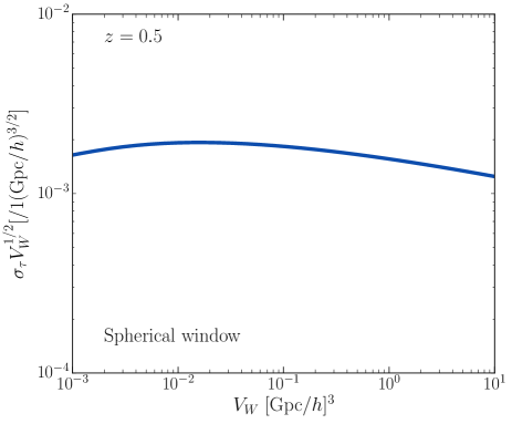
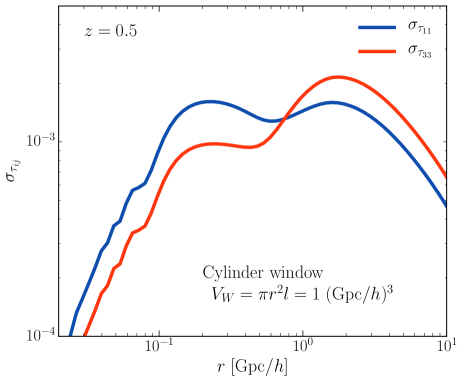
Figure 1: The rms of linear gravitational tidal field convolved with the survey window, $\sigma_{\tau ij}$ for a $\Lambda$CDM model and $z=0.5$ (see Eqs. 6 and 7). Left panel: the rms as a function of survey volume for spherical window, $V_{W}=4\pi r^{3}/3$. In this case, the tidal tensor becomes diagonal; $\sigma_{\tau}\equiv\sigma_{\tau 11}=\sigma_{\tau 22}=\sigma_{\tau 33}$. Right panel: the rms for cylinder windows of fixed volume $V_{W}=\pi r^{2}\ell=1~{}({\rm Gpc}/h)^{3}$, as a function of the radius of base circle, $r$. Here we assume that the height of cylinder is along the 3-axis (the light-of-sight) direction, and the base circle is in the plane perpendicular to the line-of-sight direction (therefore $\sigma_{\tau 11}=\sigma_{\tau 22}$). For an elongated cylinder window, i.e. a tube-like shaped survey, $\sigma_{\tau 11}$ has a greater amplitude, while $\sigma_{\tau 33}$ has a greater amplitude for a pill-like shape. When $r\sim\ell$, $\sigma_{\tau 11}\simeq\sigma_{\tau 33}$, and the linear variance has a largest amplitude.

The key quantity to characterize the effect of coherent tidal force is the variance of linear tidal field averaged over the survey window, $\sigma_{\tau}$ (Eq. 6). The left panel of Fig. 1 shows the variance for a $\Lambda$CDM model, for spherical window as a function of survey volume $V_{W}$. Other covariance term scales with $1/V_{W}$, so the curve shows the relative contribution of the coherent tidal force to the sample variance. Likewise the effect of super-survey overdensity $\sigma_{\rm b}$ (Takada and Hu, 2013), the super-survey covariance has a weak dependence on the volume. For a sufficiently large cosmological volume such as $V_{W}\gtrsim 1~{}({\rm Gpc}/h)^{3}$, $\sigma_{\tau}\sim 10^{-3}$.

As can be found from Eq. (6), the different components of the linear variance of super-survey tidal tensor, $\sigma_{\tau ij}$, depends on the shape of survey window. The right panel of Fig. 1 studies this for a cylinder window as a function of the different shape, for a fixed survey volume of $V_{W}=\pi r^{2}\ell=1~{}({\rm Gpc}/h)^{3}$. When $r\ll\ell$, a survey window corresponds to a survey being “narrow” in area coverage on the sky, but deep in redshift direction – a “tube-shaped” survey. A survey with $\ell\ll r$ corresponds to a survey being “wide” in area, but shallow in redshift – a “pill-shaped” survey. The linear variance components have different amplitudes depending on angles between the coordinate axes and the principal axes of tidal tensor. Here we consider the line-of-sight direction to lie along the 3rd-axis direction of an observer coordinate’s system and the height direction of the cylinder window ($\ell$-direction); in this case $\sigma_{\tau 11}=\sigma_{\tau{22}}$. The variance components, $\sigma_{\tau 33}\simeq\sigma_{\tau 11}$ when $r\simeq 0.7~{}{{\rm Gpc}/h}$ or equivalently $\ell\simeq r$. For either case of extreme “tube” or “pill” shape, one component $\sigma_{\tau 11}$ or $\sigma_{\tau 33}$ has a greater amplitude than the other. However, the variance amplitude gets smaller due to cancellation effect of the linear variances (also see Takada and Hu, 2013). However, the extreme cases are not desirable, because one length scale of the volume can be in the nonlinear regime, and the linear-order approximation of the super-survey modes breaks down.

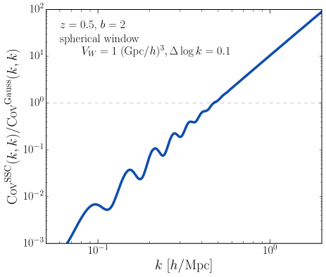
Figure 2: Shown is how the super-survey tidal force causes an increase in the sample variance in a measurement of the quadrupole power spectrum of redshift-space galaxy distribution. The curve shows the super-sample covariance (SSC) contribution to the sample variance relative to the Gaussian variance, for a survey with volume $1~{}({\rm Gpc}/h)^{3}$, at $z=0.5$ and galaxies with linear bias $b=2$ (Eqs. 27 and 29). Here we ignored the shot noise contribution due to a finite number density of galaxies. Since the Gaussian term depends on the bin width of wavenumber, we assumed a binning of $\Delta\log k=0.1$ (10 bins in one decade of wavenumber). The SSC effects causes a significant sample variance at $k\gtrsim 0.5~{}h/{\rm Mpc}$.

Fig. 2 compares the Gaussian and super-survey covariance terms in the covariance matrix of the quadrupole power spectrum, for a spherical window of $V_{W}=1~{}({\rm Gpc}/h)^{3}$ (see Eqs. 27 and 29). Here we assume a survey probing the three-dimensional distribution of galaxies at $z=0.5$ and with linear bias parameter $b=2$, which roughly resemble SDSS CMASS-type galaxies (Reid et al., 2012). Here we ignored the effect of a finite number density of the galaxies. Since the Gaussian covariance depends on the bin width of wavenumber, we employ $\Delta\log k=0.1$. Note that, in order to show the effect of the coherent tidal force on the BAO features, we employed a much finer $k$-binning to plot the curve, but used $\Delta\log k=0.1$ to compute the Gaussian term at each $k$-bin. The figure shows that the super-survey effect gives a dominant contribution to the sample variance in the weakly nonlinear regime, $k\gtrsim 0.7~{}{h/{\rm Mpc}}$.

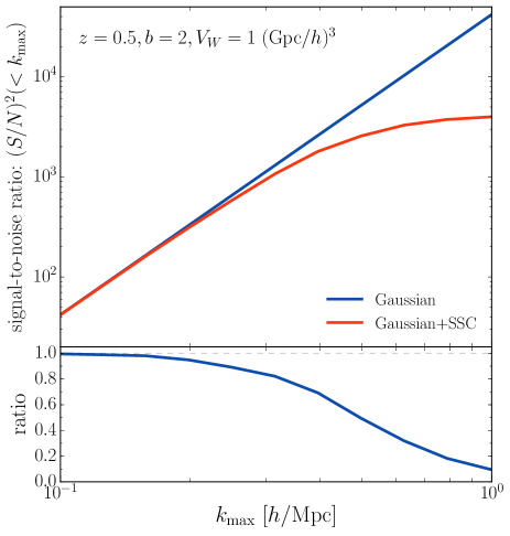
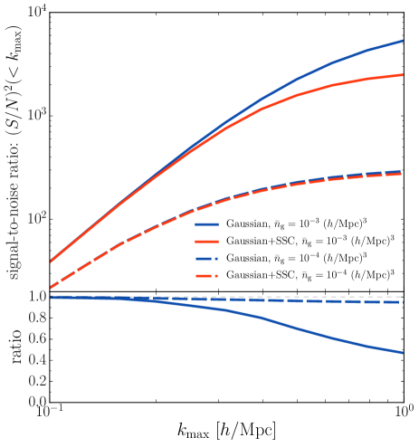
Figure 3: Cumulative signal-to-noise ratio (S/N) for a measurement of the quadrupole power spectrum, as a function of maximum wavenumber $k_{\rm max}$. We here assumed $V_{W}=1~{}({\rm Gpc}/h)^{3},z=0.5$ and $b=2$ as in the previous figure. S/N does not depend on the bin width of $k$. Left panel: The results for an infinite number density of galaxies; we ignored the shot noise contribution. The upper or lower curves in the upper plot are the results when assuming the Gaussian covariance or including the SSC contribution, respectively. The lower panel shows the ratio. Right panel: The similar plot, but for a finite number density of galaxies: $\bar{n}_{\rm g}=10^{-3}$ or $10^{-4}~{}(h/{\rm Mpc})^{3}$, respectively.

As one demonstration of the impact of the coherent tidal force on a measurement of the quadrupole power spectrum in redshift space, we study a cumulative signal-to-noise ratio, defined as

$$\left(\frac{S}{N}\right)^{2}_{\leq k_{\rm max}}\equiv\sum_{k_{i}k_{j}\in k_{\rm max}}P^{S}_{{\rm g}2W}(k_{i})\left[{\bf C}^{-1}\right]_{ij}P^{S}_{{\rm g}2W}(k_{j}),$$ (30)

where ${\bf C}^{-1}$ is the inverse of the covariance matrix, and the summation runs over all wavenumber bins up to a given maximum wavenumber $k_{\rm max}$. This quantity does not depend on the bin width. The inverse of $(S/N)$ gives a statistical precision of measuring the overall amplitude of the power spectrum, if the shape is completely known. Fig. 3 shows the results. The super-survey tidal force causes a degradation in the power spectrum measurement, at $k_{\rm max}\gtrsim\mbox{a few}~{}h/{\rm Mpc}$, and for a galaxy survey with a high number density such as $\bar{n}_{\rm g}\simeq 10^{-3}~{}(h/{\rm Mpc})^{3}$, which is the case for the WFIRST-AFTA survey (Spergel et al., 2015).

IV Discussion

We have derived a formula to describe the effect of super-survey, coherent tidal force on the redshift-space power spectrum measured in a finite volume survey. The large-scale coherent overdensity and tidal field both arise from the Hessian of the long-wavelength gravitational potential, and are of equal importance. Since the super-survey modes are not direct observables, the effects on cosmological observables need to be theoretically modeled. The super-survey tide causes a characteristic, anisotropic clustering pattern in the distribution of the tracers, in all three directions perpendicular and parallel to the line-of-sight direction (see Eq. 17). This effect appears to be exactly similar to the geometrical Alcock-Paczynski (AP) distortion as well as the redshift-space distortion effect of peculiar velocities. We then derived a formula to model the contribution of the coherent tidal force to the sample variance in a measurement of the quadrupole redshift-space power spectrum. We showed that the super-sample variance is not negligible if including the power spectrum information up to the weakly nonlinear regime, $k\gtrsim\mbox{a few}~{}h/{\rm Mpc}$ or for a galaxy survey with a high number density such as $\bar{n}_{\rm g}\simeq 10^{-3}~{}(h/{\rm Mpc})^{3}$. In our derivation, we have not yet properly included the super-survey effects on the nonlinear Kaiser factor. This can be done by using the perturbation theory, and is our future work.

For a galaxy survey with a volume coverage greater than $\sim({\rm Gpc/h})^{3}$ and $z=0.5$ as in the SDSS survey, the linear variance of super-survey tidal force $\sigma_{\tau}\sim 10^{-3}$ for a $\Lambda$CDM model. This implies that the super-survey tide causes about 0.1% anisotropy in the clustering distribution. However, the expectation value of the variance is after the angle average, compared to the variance of coherent density contrast: $\sigma_{\tau}\simeq\sqrt{4/45}\sigma_{\rm b}\simeq\sigma_{\rm b}/3.4$ (see Eq. 7). If the principal axes of the super-survey tidal tensor have an alignment to directions parallel and/or perpendicular to the line-of-sight direction, the tide could have a similar amplitude as $\delta_{\rm b}$ in a particular realization: $\tau\sim\delta_{\rm b}$ corresponding to $\sim 0.3\%$ anisotropy. Since the current state-of-the-art SDSS BOSS survey already achieved about 1% accuracy for the BAO distance measurements (Alam et al., 2016), the super-survey tide could cause a bias by an amount of the $1\sigma$ statistical error, if the SDSS survey volume is embedded into a particular region where the aligned tide has a $3\sigma$ value. Hence, it would be more important to study how the coherent tidal force could cause a bias in measurements of the cosmological distances via the AP test as well as the growth rate via the RSD effect. This requires to propagate the expected statistical accuracy of the redshift-space power spectrum measurement into parameter estimation for a given survey geometry, including marginalization over other parameters. This is our future work, and will be presented elsewhere.

The redshift-space clustering of galaxies is anisotropic by nature, and the coherent tidal force causes a similar anisotropic clustering pattern in the observed distribution. For the monopole power spectrum such as the weak lensing power spectrum, the effect disappears at the first order of $\tau_{Wij}$ due to the trace-less nature ${\rm Tr}(\tau_{Wij})=0$. There are other effects of the coherent tidal force that can be observed in principle from upcoming wide-area galaxy surveys. First, it is shown that the coherent tidal force causes a modification of dark matter halo formation via a coupling of the inertia of mass distribution in a proto-halo region with the coherent tidal force, leaving a non-local bias effect relative to the underlying matter distribution at the second order: $\partial\delta_{\rm h}/\partial(\tau_{W}^{2})=b_{\tau}$ (Chan et al., 2012; Saito et al., 2014). The non-local bias can be measured by combining measurements of the power spectrum (two-point) and bispectrum (three-point) of large-scale structure tracers. Another observable is the correlation of the large-scale tidal force with shapes of galaxies at much smaller scales, the so-called intrinsic alignments (Heavens et al., 2000; Hirata and Seljak, 2004). The intrinsic alignments are one of the major systematic effects for ongoing and upcoming weak lensing surveys. Conversely, the intrinsic alignments can be regarded as a “signal”, rather than a contaminating systematic error, and can be measured from these wide-area galaxy surveys in order to constrain the large-scale tidal force Schmidt et al. (2015); Chisari et al. (2016). Furthermore, a better understanding of the nonlinear mode coupling allows one to use a combination of the observed sub-survey modes to estimate the large-scale tidal field (Pen et al., 2012; Zhu et al., 2016a, b).

In order to realize the effect of coherent tidal force on structure formation in the deeply nonlinear regime, such as halo formation, we need to use $N$-body simulations. For this purpose, a separate universe simulation technique would be powerful; since the large-scale tidal force can be absorbed into the perturbed scale factors along each coordinate axis, $a_{W}(t)\simeq a(t)\left[1-\tau_{Wi}\right]$, we can follow the full nonlinear mode coupling of the large-scale tide with sub-box modes by running $N$-body simulations in the perturbed background. For the coherent overdensity $\delta_{\rm b}$, the effect for a $\Lambda$CDM model can be absorbed as an apparent curvature, even if the global background is flat. Several works have developed the separate universe simulation technique to study the mode coupling effect of $\delta_{\rm b}$ with sub-box modes (Li et al., 2014a, b; Wagner et al., 2015; Baldauf et al., 2016; Lazeyras et al., 2016; Li et al., 2016). The separate universe simulation allows for a better calibration of various effects such as the super-sample covariance and the local halo bias, without running a large number of huge box simulations. In a very similar way we believe that the separate universe simulation technique can be applied to the large-scale tidal effect. Recently Ip and Schmidt (2017) developed a unified formula to model the effect of the coherent tidal force on the evolution of sub-survey modes within the framework of general relativity. However, there are in general two contributions to the large-scale tidal field: the internal tidal force arising from the anisotropic matter distribution within a finite-volume boundary and the external tidal force that is not specified by the internal boundary conditions (also see Bond and Myers, 1996; Hui and Bertschinger, 1996). Nevertheless, as long as we are interested in the effects of the linear tidal force, it would be possible to develop a separate universe simulation technique to include the large-scale tide in the simulation as well as to study the effect on nonlinear structure formation. If this is true, the separate universe simulations would give us a better way to calibrate the large-scale tidal effects on various cosmological observables. This is in progress and will be presented elsewhere.

Acknowledgments.– We thank Matias Zaldarriaga, Fabian Schmidt, Atsushi Taruya and Tobias Baldauf for useful discussion, and we also thank to YITP, Kyoto University for their warm hospitality. KA is supported by the Advanced Leading Graduate Course for Photon Science at the University of Tokyo. MT is supported by World Premier International Research Center Initiative (WPI Initiative), MEXT, Japan, by the FIRST program “Subaru Measurements of Images and Redshifts (SuMIRe)”, CSTP, Japan. MT is supported by Grant-in-Aid for Scientific Research from the JSPS Promotion of Science (No. 23340061, 26610058, and 15H05893), MEXT Grant-in-Aid for Scientific Research on Innovative Areas (No. 15K21733, 15H05892) and by JSPS Program for Advancing Strategic International Networks to Accelerate the Circulation of Talented Researchers.

Appendix A Takada & Hu derivation of power spectrum response to super-survey modes

In this appendix we derive the responses of the real-space power spectrum to the long-wavelength tidal force, based on the formulation in Takada and Hu (2013).

Taking into account the survey window, The observed field of the matter fluctuation field can be defined as

$$\delta_{W}({\bf x})=\delta({\bf x})W({\bf x}),$$ (31)

whose Fourier transform is a convolution

$$\tilde{\delta}_{W}({\bf k})=\int\!\!\frac{d^{3}{\bf q}}{(2\pi)^{3}}~{}\tilde{W}({\bf q})\tilde{\delta}({\bf k}-{\bf q}).$$ (32)

In order to study how the large-scale tide causes an anisotropic modulation in the measured power spectrum, let us define an estimator of the two-dimensional power spectrum of wavevector ${\bf k}$ as

$$\hat{P}({\bf k})=\frac{1}{V_{W}}\tilde{\delta}_{W}({\bf k})\tilde{\delta}_{W}(-{\bf k}),$$ (33)

Note that the wavevector bin ${\bf k}$ can be finite, compared to the fundamental mode of a survey, $k_{f}\simeq 2\pi/L$, and in that case the above estimator is defined from a sum of the modes within the bin width. The power spectrum estimator satisfies a parity invariance:

$$\hat{P}({\bf k})=\hat{P}(-{\bf k}).$$ (34)

The ensemble average of the estimator is found to recover the underlying true power spectrum

$$\left\langle\hat{P}({\bf k})\right\rangle = \frac{1}{V_{W}}\int\!\!\frac{\mathrm{d}^{3}{\bf q}}{(2\pi)^{3}}~{}|\tilde{W}({\bf q})|^{2}P({\bf k}-{\bf q})\simeq P({\bf k})\frac{1}{V_{W}}\int\!\!\frac{\mathrm{d}^{3}{\bf q}}{(2\pi)^{3}}~{}|\tilde{W}({\bf q})|^{2}=P({\bf k})$$ (35)

Here we have used that $P({\bf k}-{\bf q})\simeq P({\bf k})$ over the integration range of $d^{3}{\bf q}$ which the window function supports and also assumed that $P({\bf k})$ is not a rapidly varying function within the $k$-bin. In the third equality on the r.h.s., we have used the general identity for the window function:

$$V_{W}=\int\!d^{3}{\bf x}~{}W^{n}({\bf x})=\int\!\left[\prod_{a=1}^{n}\frac{d^{3}{\bf q}_{a}}{(2\pi)^{3}}\tilde{W}({\bf q}_{a})\right](2\pi)^{3}\delta^{3}_{D}({\bf q}_{1\ldots n}),$$ (36)

where ${\bf q}_{1\ldots n}={\bf q}_{1}+\ldots{\bf q}_{n}$ here and below. For $n=2$, $V_{W}=\int|\tilde{W}({\bf q})|^{2}d^{3}{\bf q}/(2\pi)^{3}$.

As we have discussed, the super-survey modes affect the power spectrum measured in a finite-volume survey region. Hence, when a given survey volume has super-survey modes of $\delta_{\rm b}$ and $\tau_{Wij}$, the effects on power spectrum measured in the survey realization are expressed as

$$P({\bf k};\delta_{\rm b},\tau_{W})\simeq P(k)+\frac{\partial P(k)}{\partial\delta_{\rm b}}\delta_{\rm b}+\frac{\partial P(k)}{\partial\tau_{Wij}}\tau_{Wij}.$$ (37)

Here $\partial P(k)/\partial\delta_{\rm b}$ and $\partial P(k)/\partial\tau_{Wij}$ are the responses of the power spectrum to the super-survey modes, $\delta_{\rm b}$ and $\tau_{Wij}$, respectively. Here we consider the power spectrum responses at the leading order of the super-survey modes, or in other words we ignored the responses at the higher orders of $O(\delta_{\rm b}^{2},\tau_{W}^{2})$. The ensemble average of the above power spectrum, which is equivalent to the average of the power spectrum estimator for different survey regions, is

$$\left\langle P({\bf k};\delta_{\rm b},\tau_{W})\right\rangle=P(k)+\frac{\partial P(k)}{\partial\delta_{\rm b}}\left\langle\delta_{\rm b}\right\rangle+\frac{\partial P(k)}{\partial\tau_{Wij}}\left\langle\tau_{Wij}\right\rangle=P({\bf k}),$$ (38)

where we used $\left\langle\delta_{\rm b}\right\rangle=\left\langle\tau_{Wij}\right\rangle=0$. Thus the ensemble average of the power spectrum estimator recovers the true power spectrum in the global universe.

Now let us consider the covariance matrix of the power spectrum estimator (Eq. 33):

$$C({\bf k},{\bf k}^{\prime})=\left\langle\hat{P}({\bf k})\hat{P}({\bf k}^{\prime})\right\rangle-P({\bf k})P({\bf k}^{\prime}).$$ (39)

Inserting Eq. (37) into the above equation leads us to find a formal expression of the super-sample covariance due to $\delta_{\rm b}$ and $\tau_{W}$:

$$C^{\rm SSC}({\bf k},{\bf k}^{\prime})=\sigma_{\rm b}^{2}\frac{\partial P(k)}{\partial\delta_{\rm b}}\frac{\partial P(k^{\prime})}{\partial\delta_{\rm b}}+\left\langle\tau_{Wij}\tau_{Wlm}\right\rangle\frac{\partial P(k)}{\partial\tau_{Wij}}\frac{\partial P(k^{\prime})}{\partial\tau_{Wlm}},$$ (40)

where we have assumed $\left\langle\delta_{\rm b}\tau_{Wij}\right\rangle\simeq 0$ for a reasonably symmetric survey window.

Following the formulation in Takada and Hu (2013) (Li et al., 2014b), we advocate that the squeezed trispectrum can be characterized by the responses of the power spectrum to the super-survey modes as

$$\lim_{q\rightarrow 0}\left[T^{\rm PT}({\bf k},-{\bf k}+{\bf q},{\bf k}^{\prime},-{\bf k}-{\bf q})-T^{\rm PT}({\bf k},-{\bf k},{\bf k}^{\prime},-{\bf k}^{\prime})\right]\simeq P^{L}(q)\left[\frac{\partial P(k)}{\partial\delta_{\rm b}}+\tau_{Wij}\frac{\partial P(k)}{\partial\tau_{Wij}}\right]\left[\frac{\partial P(k^{\prime})}{\partial\delta_{\rm b}}+\tau_{Wlm}\frac{\partial P(k^{\prime})}{\partial\tau_{Wlm}}\right],$$ (41)

where the Fourier modes ${\bf q}$ are super-survey modes satisfying $k,k^{\prime}\gg q$. Using the perturbation theory (Bernardeau et al., 2002), we can compute the squeezed trispectrum contribution:

$$C^{\rm SSC}({\bf k},{\bf k}^{\prime}) = \frac{1}{V_{W}^{2}}\int\!\!\frac{\mathrm{d}^{2}{\bf q}}{(2\pi)^{3}}|\tilde{W}({\bf q})|^{2}\left[T^{\rm PT}({\bf k},-{\bf k}+{\bf q},{\bf k}^{\prime},-{\bf k}^{\prime}-{\bf q})-T^{\rm PT}({\bf k},-{\bf k},{\bf k}^{\prime},-{\bf k}^{\prime})\right].$$ (42)

$T^{\rm PT}$ is the tree-level trispectrum, defined as

$$\left\langle\delta({\bf k}_{1})\delta({\bf k}_{2})\delta({\bf k}_{3})\delta({\bf k}_{4})\right\rangle_{c}=(2\pi)^{3}\delta_{D}^{3}({\bf k}_{1234})T^{\rm PT}({\bf k}_{1},{\bf k}_{2},{\bf k}_{3},{\bf k}_{4}).$$ (43)

where

$$T^{\rm PT}({\bf k}_{1},{\bf k}_{2},{\bf k}_{3},{\bf k}_{4}) = 4\left[F_{2}({\bf k}_{13},-{\bf k}_{1})F_{2}({\bf k}_{13},{\bf k}_{2})P^{{\rm L}}(k_{13})P^{{\rm L}}(k_{1})P^{{\rm L}}(k_{2})+11{\rm perm.}\right]$$ (44)

$$+6\left[F_{3}({\bf k}_{1},{\bf k}_{2},{\bf k}_{3})P^{{\rm L}}(k_{1})P^{{\rm L}}(k_{2})P^{{\rm L}}(k_{3})+\mbox{3 perm.}\right],$$

with the Fourier kernels defined as

$$F_{2}({\bf k}_{1},{\bf k}_{2}) = \frac{5}{7}+\frac{1}{2}\left(\frac{1}{k_{1}^{2}}+\frac{1}{k_{2}^{2}}\right)({\bf k}_{1}\cdot{\bf k}_{2})+\frac{2}{7}\frac{({\bf k}_{1}\cdot{\bf k}_{2})^{2}}{k_{1}^{2}k_{2}^{2}},$$ (45)

and the definition of $F_{3}$ is given by Eq. (31) in Takada and Hu (2013), but the term involving $F_{3}$ is not relevant for the following calculation.

Inserting Eqs. (44) and (45) into Eq. (42) leads to

$$C^{\rm SSC}({\bf k},{\bf k}^{\prime}) \simeq \frac{1}{V_{W}^{2}}\int\!\!\frac{\mathrm{d}^{3}{\bf q}}{(2\pi)^{3}}|\tilde{W}({\bf q})|^{2}4P^{L}(q)\left[P^{L}(k)F_{2}({\bf q},-{\bf k})+P^{L}(|{\bf k}-{\bf q}|)F_{2}({\bf q},{\bf k}-{\bf q})\right]$$

$$\hskip 100.00015pt\times\left[P^{L}(k^{\prime})F_{2}({\bf q},{\bf k}^{\prime})+P^{L}(|{\bf k}^{\prime}+{\bf q}|)F_{2}(-{\bf q},{\bf k}^{\prime}+{\bf q})\right],$$

To further proceed the calculation, we need to care the fact that the mode coupling kernel $F_{2}$ has a pole. More especially, under the fact $k,k^{\prime}\gg q$, we need to use the following expansion such as

$$P^{L}(|{\bf k}-{\bf q}|)F_{2}({\bf q},{\bf k}-{\bf q})\simeq\left[P(k)-\frac{\partial P(k)}{\partial k}({\bf k}\cdot{\bf q})\right]\left[\frac{5}{7}+\frac{1}{2}\left(\frac{1}{q^{2}}+\frac{1}{k^{2}}\right)\left({\bf k}\cdot{\bf q}-q^{2}\right)+\frac{({\bf k}\cdot{\bf q}-q^{2})^{2}}{q^{2}k^{2}}\right].$$ (47)

Then we can find that the super-sample covariance can be computed as

$$C^{\rm SSC}({\bf k},{\bf k}^{\prime}) \simeq \sigma_{\rm b}^{2}\left[\frac{47}{21}-\frac{1}{3}\frac{\partial\ln P(k)}{\partial\ln k}\right]\left[\frac{47}{21}-\frac{1}{3}\frac{\partial\ln P(k^{\prime})}{\partial\ln k^{\prime}}\right]P^{L}(k)P^{L}(k^{\prime})$$ (48)

$$+\left\langle\tau_{Wij}\tau_{Wlm}\right\rangle\hat{k}_{i}\hat{k}_{j}\hat{k}_{l}^{\prime}\hat{k}_{m}^{\prime}\left[\frac{8}{7}-\frac{\partial\ln P(k)}{\partial\ln k}\right]\left[\frac{8}{7}-\frac{\partial\ln P(k^{\prime})}{\partial\ln k^{\prime}}\right]P^{L}(k)P^{L}(k^{\prime}),$$

where $\hat{{\bf k}}={\bf k}/k$. To arrive at this equation, we used the following identities for the ${\bf q}$-integration:

$$\int\!\!\frac{\mathrm{d}^{3}{\bf q}}{(2\pi)^{3}}~{}|\tilde{W}({\bf q})|^{2}P^{L}(q) = \sigma_{\rm b}^{2}$$ (49)

$$\int\!\!\frac{\mathrm{d}^{3}{\bf q}}{(2\pi)^{3}}~{}|\tilde{W}({\bf q})|^{2}P^{L}(q)q_{i}q_{j} = \int\!\!\frac{\mathrm{d}^{3}{\bf q}}{(2\pi)^{3}}~{}|\tilde{W}({\bf q})|^{2}P^{L}(q)\left[\left(q_{i}q_{j}-\frac{\delta^{K}_{ij}}{3}\right)+\frac{\delta^{K}_{ij}}{3}\right]$$ (50)

$$= \left\langle\delta_{\rm b}\tau_{Wij}\right\rangle+\frac{\delta^{K}_{ij}}{3}\sigma_{{\rm b}}^{2}$$

$$\simeq \frac{\delta^{K}_{ij}}{3}\sigma_{{\rm b}}^{2}$$

$$\int\!\!\frac{\mathrm{d}^{3}{\bf q}}{(2\pi)^{3}}~{}|\tilde{W}({\bf q})|^{2}P^{L}(q)q_{i}q_{j}q_{l}q_{m} \simeq \int\!\!\frac{\mathrm{d}^{3}{\bf q}}{(2\pi)^{3}}~{}|\tilde{W}({\bf q})|^{2}P^{L}(q)\left[\left(q_{i}q_{j}-\frac{\delta^{K}_{ij}}{3}\right)\left(q_{l}q_{m}-\frac{\delta^{K}_{lm}}{3}\right)+\frac{\delta^{K}_{ij}\delta^{K}_{lm}}{9}\right]$$ (51)

$$= \left\langle\tau_{Wij}\tau_{Wlm}\right\rangle+\frac{\delta^{K}_{ij}\delta^{K}_{lm}}{9}\sigma_{{\rm b}}^{2}.$$

Note that we also used the fact that terms involving the moments with an odd power of $q_{i}$ or equivalently an odd power of $k_{i}$ are vanishing under the parity invariance conditions of ${\bf k}\leftrightarrow-{\bf k}$ and ${\bf k}^{\prime}\leftrightarrow-{\bf k}^{\prime}$.

Comparing Eqs. (40) and (48) leads us to find that the power spectrum response can be given as

$$P({\bf k};\delta_{\rm b},\tau_{W})\simeq P(k)+\delta_{\rm b}\left[\frac{47}{21}-\frac{1}{3}\frac{\partial\ln P(k)}{\partial\ln k}\right]P(k)+\hat{k}_{i}\hat{k}_{j}\tau_{Wij}\left[\frac{8}{7}-\frac{\partial\ln P(k)}{\partial\ln k}\right]P(k).$$ (52)

References

- Seo and Eisenstein (2003) H. Seo and D. J. Eisenstein, Astrophys. J. 598, 720 (2003), arXiv:astro-ph/0307460 .
- Hu and Haiman (2003) W. Hu and Z. Haiman, Phys. Rev. D 68, 063004 (2003), astro-ph/0306053 .
- Eisenstein et al. (2005) D. J. Eisenstein et al., Astrophys. J. 633, 560 (2005), arXiv:astro-ph/0501171 .
- Aubourg et al. (2015) É. Aubourg, S. Bailey, J. E. Bautista, F. Beutler, V. Bhardwaj, D. Bizyaev, M. Blanton, M. Blomqvist, A. S. Bolton, J. Bovy, H. Brewington, J. Brinkmann, J. R. Brownstein, A. Burden, N. G. Busca, W. Carithers, C.-H. Chuang, J. Comparat, R. A. C. Croft, A. J. Cuesta, K. S. Dawson, T. Delubac, D. J. Eisenstein, A. Font-Ribera, J. Ge, J.-M. Le Goff, S. G. A. Gontcho, J. R. Gott, J. E. Gunn, H. Guo, J. Guy, J.-C. Hamilton, S. Ho, K. Honscheid, C. Howlett, D. Kirkby, F. S. Kitaura, J.-P. Kneib, K.-G. Lee, D. Long, R. H. Lupton, M. V. Magaña, V. Malanushenko, E. Malanushenko, M. Manera, C. Maraston, D. Margala, C. K. McBride, J. Miralda-Escudé, A. D. Myers, R. C. Nichol, P. Noterdaeme, S. E. Nuza, M. D. Olmstead, D. Oravetz, I. Pâris, N. Padmanabhan, N. Palanque-Delabrouille, K. Pan, M. Pellejero-Ibanez, W. J. Percival, P. Petitjean, M. M. Pieri, F. Prada, B. Reid, J. Rich, N. A. Roe, A. J. Ross, N. P. Ross, G. Rossi, J. A. Rubiño-Martín, A. G. Sánchez, L. Samushia, R. T. G. Santos, C. G. Scóccola, D. J. Schlegel, D. P. Schneider, H.-J. Seo, E. Sheldon, A. Simmons, R. A. Skibba, A. Slosar, M. A. Strauss, D. Thomas, J. L. Tinker, R. Tojeiro, J. A. Vazquez, M. Viel, D. A. Wake, B. A. Weaver, D. H. Weinberg, W. M. Wood-Vasey, C. Yèche, I. Zehavi, G.-B. Zhao, and BOSS Collaboration, Phys. Rev. D 92, 123516 (2015), arXiv:1411.1074 .
- Zhang et al. (2007) P. Zhang, M. Liguori, R. Bean, and S. Dodelson, Physical Review Letters 99, 141302 (2007), arXiv:0704.1932 .
- Hu et al. (1998) W. Hu, D. J. Eisenstein, and M. Tegmark, Physical Review Letters 80, 5255 (1998), astro-ph/9712057 .
- Takada et al. (2006) M. Takada, E. Komatsu, and T. Futamase, Phys. Rev. D 73, 083520 (2006), arXiv:astro-ph/0512374 .
- Saito et al. (2008) S. Saito, M. Takada, and A. Taruya, Physical Review Letters 100, 191301 (2008), arXiv:0801.0607 .
- Dalal et al. (2008) N. Dalal, O. Doré, D. Huterer, and A. Shirokov, Phys. Rev. D 77, 123514 (2008), arXiv:arXiv:0710.4560 .
- Carbone et al. (2011) C. Carbone, A. Mangilli, and L. Verde, JCAP 9, 028 (2011), arXiv:1107.1211 [astro-ph.CO] .
- Arkani-Hamed and Maldacena (2015) N. Arkani-Hamed and J. Maldacena, ArXiv e-prints (2015), arXiv:1503.08043 [hep-th] .
- Takada and Doré (2015) M. Takada and O. Doré, Phys. Rev. D 92, 123518 (2015), arXiv:1508.02469 .
- Hlozek et al. (2015) R. Hlozek, D. Grin, D. J. E. Marsh, and P. G. Ferreira, Phys. Rev. D 91, 103512 (2015), arXiv:1410.2896 .
- Reid et al. (2012) B. A. Reid, L. Samushia, M. White, W. J. Percival, M. Manera, N. Padmanabhan, A. J. Ross, A. G. Sánchez, S. Bailey, D. Bizyaev, A. S. Bolton, H. Brewington, J. Brinkmann, J. R. Brownstein, A. J. Cuesta, D. J. Eisenstein, J. E. Gunn, K. Honscheid, E. Malanushenko, V. Malanushenko, C. Maraston, C. K. McBride, D. Muna, R. C. Nichol, D. Oravetz, K. Pan, R. de Putter, N. A. Roe, N. P. Ross, D. J. Schlegel, D. P. Schneider, H.-J. Seo, A. Shelden, E. S. Sheldon, A. Simmons, R. A. Skibba, S. Snedden, M. E. C. Swanson, D. Thomas, J. Tinker, R. Tojeiro, L. Verde, D. A. Wake, B. A. Weaver, D. H. Weinberg, I. Zehavi, and G.-B. Zhao, Mon. Not. Roy. Astron. Soc. 426, 2719 (2012), arXiv:1203.6641 .
- Alam et al. (2016) S. Alam, M. Ata, S. Bailey, F. Beutler, D. Bizyaev, J. A. Blazek, A. S. Bolton, J. R. Brownstein, A. Burden, C.-H. Chuang, J. Comparat, A. J. Cuesta, K. S. Dawson, D. J. Eisenstein, S. Escoffier, H. Gil-Marín, J. N. Grieb, N. Hand, S. Ho, K. Kinemuchi, D. Kirkby, F. Kitaura, E. Malanushenko, V. Malanushenko, C. Maraston, C. K. McBride, R. C. Nichol, M. D. Olmstead, D. Oravetz, N. Padmanabhan, N. Palanque-Delabrouille, K. Pan, M. Pellejero-Ibanez, W. J. Percival, P. Petitjean, F. Prada, A. M. Price-Whelan, B. A. Reid, S. A. Rodríguez-Torres, N. A. Roe, A. J. Ross, N. P. Ross, G. Rossi, J. A. Rubiño-Martín, A. G. Sánchez, S. Saito, S. Salazar-Albornoz, L. Samushia, S. Satpathy, C. G. Scóccola, D. J. Schlegel, D. P. Schneider, H.-J. Seo, A. Simmons, A. Slosar, M. A. Strauss, M. E. C. Swanson, D. Thomas, J. L. Tinker, R. Tojeiro, M. Vargas Magaña, J. A. Vazquez, L. Verde, D. A. Wake, Y. Wang, D. H. Weinberg, M. White, W. M. Wood-Vasey, C. Yèche, I. Zehavi, Z. Zhai, and G.-B. Zhao, ArXiv e-prints (2016), arXiv:1607.03155 .
- Takada et al. (2014) M. Takada, R. S. Ellis, M. Chiba, J. E. Greene, H. Aihara, N. Arimoto, K. Bundy, J. Cohen, O. Doré, G. Graves, J. E. Gunn, T. Heckman, C. M. Hirata, P. Ho, J.-P. Kneib, O. L. Fèvre, L. Lin, S. More, H. Murayama, T. Nagao, M. Ouchi, M. Seiffert, J. D. Silverman, L. Sodré, D. N. Spergel, M. A. Strauss, H. Sugai, Y. Suto, H. Takami, and R. Wyse, PASJ 66, R1 (2014), arXiv:1206.0737 .
- DESI Collaboration et al. (2016) DESI Collaboration, A. Aghamousa, J. Aguilar, S. Ahlen, S. Alam, L. E. Allen, C. Allende Prieto, J. Annis, S. Bailey, C. Balland, and et al., ArXiv e-prints (2016), arXiv:1611.00036 [astro-ph.IM] .
- Note (1) http://sci.esa.int/euclid/.
- Doré et al. (2014) O. Doré, J. Bock, M. Ashby, P. Capak, A. Cooray, R. de Putter, T. Eifler, N. Flagey, Y. Gong, S. Habib, K. Heitmann, C. Hirata, W.-S. Jeong, R. Katti, P. Korngut, E. Krause, D.-H. Lee, D. Masters, P. Mauskopf, G. Melnick, B. Mennesson, H. Nguyen, K. Öberg, A. Pullen, A. Raccanelli, R. Smith, Y.-S. Song, V. Tolls, S. Unwin, T. Venumadhav, M. Viero, M. Werner, and M. Zemcov, ArXiv e-prints (2014), arXiv:1412.4872 .
- Spergel et al. (2015) D. Spergel, N. Gehrels, C. Baltay, D. Bennett, J. Breckinridge, M. Donahue, A. Dressler, B. S. Gaudi, T. Greene, O. Guyon, C. Hirata, J. Kalirai, N. J. Kasdin, B. Macintosh, W. Moos, S. Perlmutter, M. Postman, B. Rauscher, J. Rhodes, Y. Wang, D. Weinberg, D. Benford, M. Hudson, W.-S. Jeong, Y. Mellier, W. Traub, T. Yamada, P. Capak, J. Colbert, D. Masters, M. Penny, D. Savransky, D. Stern, N. Zimmerman, R. Barry, L. Bartusek, K. Carpenter, E. Cheng, D. Content, F. Dekens, R. Demers, K. Grady, C. Jackson, G. Kuan, J. Kruk, M. Melton, B. Nemati, B. Parvin, I. Poberezhskiy, C. Peddie, J. Ruffa, J. K. Wallace, A. Whipple, E. Wollack, and F. Zhao, ArXiv e-prints (2015), arXiv:1503.03757 [astro-ph.IM] .
- Bernardeau et al. (2002) F. Bernardeau, S. Colombi, E. Gaztañaga, and R. Scoccimarro, Phys. Rep. 367, 1 (2002), arXiv:astro-ph/0112551 .
- Hu and Kravtsov (2003) W. Hu and A. V. Kravtsov, Astrophys. J. 584, 702 (2003), arXiv:astro-ph/0203169 .
- Hamilton et al. (2006) A. J. S. Hamilton, C. D. Rimes, and R. Scoccimarro, Mon. Not. Roy. Astron. Soc. 371, 1188 (2006), arXiv:astro-ph/0511416 .
- Takada and Bridle (2007) M. Takada and S. Bridle, New Journal of Physics 9, 446 (2007), arXiv:arXiv:0705.0163 .
- Takada and Jain (2009) M. Takada and B. Jain, Mon. Not. Roy. Astron. Soc. 395, 2065 (2009), arXiv:0810.4170 .
- Sato et al. (2009) M. Sato, T. Hamana, R. Takahashi, M. Takada, N. Yoshida, T. Matsubara, and N. Sugiyama, Astrophys. J. 701, 945 (2009), arXiv:0906.2237 [astro-ph.CO] .
- Sherwin and Zaldarriaga (2012) B. D. Sherwin and M. Zaldarriaga, Phys. Rev. D 85, 103523 (2012), arXiv:1202.3998 [astro-ph.CO] .
- Kayo et al. (2013) I. Kayo, M. Takada, and B. Jain, Mon. Not. Roy. Astron. Soc. 429, 344 (2013), arXiv:1207.6322 [astro-ph.CO] .
- Takada and Hu (2013) M. Takada and W. Hu, Phys. Rev. D 87, 123504 (2013), arXiv:1302.6994 [astro-ph.CO] .
- Takada and Spergel (2014) M. Takada and D. N. Spergel, Mon. Not. Roy. Astron. Soc. 441, 2456 (2014), arXiv:1307.4399 .
- Schaan et al. (2014) E. Schaan, M. Takada, and D. N. Spergel, Phys. Rev. D 90, 123523 (2014), arXiv:1406.3330 .
- Li et al. (2014a) Y. Li, W. Hu, and M. Takada, Phys. Rev. D 89, 083519 (2014a), arXiv:1401.0385 .
- Li et al. (2014b) Y. Li, W. Hu, and M. Takada, Phys. Rev. D 90, 103530 (2014b), arXiv:1408.1081 .
- Mohammed and Seljak (2014) I. Mohammed and U. Seljak, Mon. Not. Roy. Astron. Soc. 445, 3382 (2014), arXiv:1407.0060 .
- Mohammed et al. (2016) I. Mohammed, U. Seljak, and Z. Vlah, ArXiv e-prints (2016), arXiv:1607.00043 .
- Dai et al. (2015) L. Dai, E. Pajer, and F. Schmidt, JCAP 10, 059 (2015), arXiv:1504.00351 .
- Shirasaki et al. (2016) M. Shirasaki, M. Takada, H. Miyatake, R. Takahashi, T. Hamana, T. Nishimichi, and R. Murata, ArXiv e-prints (2016), arXiv:1607.08679 .
- McDonald (2003) P. McDonald, Astrophys. J. 585, 34 (2003), astro-ph/0108064 .
- Sirko (2005) E. Sirko, Astrophys. J. 634, 728 (2005), arXiv:astro-ph/0503106 .
- Gnedin et al. (2011) N. Y. Gnedin, A. V. Kravtsov, and D. H. Rudd, Astrophys.J.Suppl. 194, 46 (2011), arXiv:1104.1428 [astro-ph.CO] .
- Baldauf et al. (2011) T. Baldauf, U. Seljak, L. Senatore, and M. Zaldarriaga, JCAP 1110, 031 (2011), arXiv:1106.5507 [astro-ph.CO] .
- Wagner et al. (2015) C. Wagner, F. Schmidt, C.-T. Chiang, and E. Komatsu, Mon. Not. Roy. Astron. Soc. 448, L11 (2015), arXiv:1409.6294 .
- Erickcek et al. (2008) A. L. Erickcek, M. Kamionkowski, and S. M. Carroll, Phys. Rev. D 78, 123520 (2008), arXiv:0806.0377 .
- White et al. (2013) J. White, M. Minamitsuji, and M. Sasaki, JCAP 9, 015 (2013), arXiv:1306.6186 [astro-ph.CO] .
- Creminelli et al. (2013) P. Creminelli, A. Joyce, J. Khoury, and M. Simonović, JCAP 4, 020 (2013), arXiv:1212.3329 [hep-th] .
- Ip and Schmidt (2017) H. Y. Ip and F. Schmidt, JCAP 2, 025 (2017), arXiv:1610.01059 .
- Eisenstein and Loeb (1995) D. J. Eisenstein and A. Loeb, Astrophys. J. 439, 520 (1995), astro-ph/9405012 .
- Hui and Bertschinger (1996) L. Hui and E. Bertschinger, Astrophys. J. 471, 1 (1996), astro-ph/9508114 .
- Bond and Myers (1996) J. R. Bond and S. T. Myers, Astrophys. J. Suppl. 103, 1 (1996).
- Dodelson (2003) S. Dodelson, Modern cosmology / Scott Dodelson. Amsterdam (Netherlands): Academic Press. ISBN 0-12-219141-2, 2003, XIII + 440 p. (2003).
- Zel’dovich (1970) Y. B. Zel’dovich, Astronomy & Astrophysics 5, 84 (1970).
- Matsubara (2008) T. Matsubara, Phys. Rev. D 78, 083519 (2008), arXiv:0807.1733 .
- Alcock and Paczynski (1979) C. Alcock and B. Paczynski, Nature (London) 281, 358 (1979).
- Kaiser (1987) N. Kaiser, Mon. Not. Roy. Astron. Soc. 227, 1 (1987).
- Baldauf et al. (2016) T. Baldauf, U. Seljak, L. Senatore, and M. Zaldarriaga, JCAP 9, 007 (2016), arXiv:1511.01465 .
- Scoccimarro et al. (1999) R. Scoccimarro, M. Zaldarriaga, and L. Hui, Astrophys. J. 527, 1 (1999), arXiv:astro-ph/9901099 .
- Guzik et al. (2010) J. Guzik, B. Jain, and M. Takada, Phys. Rev. D 81, 023503 (2010), arXiv:0906.2221 [astro-ph.CO] .
- Hinshaw et al. (2012) G. Hinshaw, D. Larson, E. Komatsu, D. N. Spergel, C. L. Bennett, J. Dunkley, M. R. Nolta, M. Halpern, R. S. Hill, N. Odegard, L. Page, K. M. Smith, J. L. Weiland, B. Gold, N. Jarosik, A. Kogut, M. Limon, S. S. Meyer, G. S. Tucker, E. Wollack, and E. L. Wright, ArXiv e-prints (2012), arXiv:1212.5226 [astro-ph.CO] .
- Chan et al. (2012) K. C. Chan, R. Scoccimarro, and R. K. Sheth, Phys. Rev. D 85, 083509 (2012), arXiv:1201.3614 [astro-ph.CO] .
- Saito et al. (2014) S. Saito, T. Baldauf, Z. Vlah, U. Seljak, T. Okumura, and P. McDonald, Phys. Rev. D 90, 123522 (2014), arXiv:1405.1447 .
- Heavens et al. (2000) A. Heavens, A. Refregier, and C. Heymans, Mon. Not. Roy. Astron. Soc. 319, 649 (2000), astro-ph/0005269 .
- Hirata and Seljak (2004) C. M. Hirata and U. Seljak, Phys. Rev. D 70, 063526 (2004), arXiv:astro-ph/0406275 .
- Schmidt et al. (2015) F. Schmidt, N. E. Chisari, and C. Dvorkin, JCAP 10, 032 (2015), arXiv:1506.02671 .
- Chisari et al. (2016) N. E. Chisari, C. Dvorkin, F. Schmidt, and D. N. Spergel, Phys. Rev. D 94, 123507 (2016), arXiv:1607.05232 .
- Pen et al. (2012) U.-L. Pen, R. Sheth, J. Harnois-Deraps, X. Chen, and Z. Li, ArXiv e-prints (2012), arXiv:1202.5804 [astro-ph.CO] .
- Zhu et al. (2016a) H.-M. Zhu, U.-L. Pen, Y. Yu, X. Er, and X. Chen, Phys. Rev. D 93, 103504 (2016a), arXiv:1511.04680 .
- Zhu et al. (2016b) H.-M. Zhu, U.-L. Pen, Y. Yu, and X. Chen, ArXiv e-prints (2016b), arXiv:1610.07062 .
- Lazeyras et al. (2016) T. Lazeyras, C. Wagner, T. Baldauf, and F. Schmidt, JCAP 2, 018 (2016), arXiv:1511.01096 .
- Li et al. (2016) Y. Li, W. Hu, and M. Takada, Phys. Rev. D 93, 063507 (2016), arXiv:1511.01454 .