Optimally Leveraging Density and Locality
to Support LIMIT Queries

Abstract

Existing database systems are not optimized for queries with a LIMIT clause—operating instead in an all-or-nothing manner. In this paper, we propose a fast LIMIT query evaluation engine, called NeedleTail, aimed at letting analysts browse a small sample of the query results on large datasets as quickly as possible, independent of the overall size of the result set. NeedleTail introduces density maps, a lightweight in-memory indexing structure, and a set of efficient algorithms (with desirable theoretical guarantees) to quickly locate promising blocks, trading off locality and density. In settings where the samples are used to compute aggregates, we extend techniques from survey sampling to mitigate the bias in our samples. Our experimental results demonstrate that NeedleTail returns results 4$\times$ faster on HDDs and 9$\times$ faster on SSDs on average, while occupying up to 23$\times$ less memory than existing techniques.

1 Introduction

Users of databases are frequently interested in retrieving only a small subset of records that satisfy a query, e.g., by specifying a LIMIT clause in a SQL query. Although there has been extensive work on top-k queries that retrieve the largest or smallest results in a result set, or that tries to provide a random sample of results, there has been relatively little work on so-called any-$k$ queries that simply retrieve a few results without any requirements about the ordering or randomness of the results.

Any-$k$ has many applications in exploratory data analysis. When exploring new or unfamiliar datasets, users often issue arbitrary queries, examine a subset or sample (a “screenful”) of records, and incrementally and re-issue their queries based on observations from this sample [59, 29]. To support this form of exploratory browsing, many popular SQL IDEs implicitly limit the number of result records displayed, recognizing the fact that users often do not need to, nor do they have the time to see all of the result records. For example, phpMyAdmin for MySQL has a MaxRows configuration parameter; pgAdmin for PostgreSQL has a rowset size parameter; and SQL Developer for Oracle has a array fetch size parameter. Even outside of the context of SQL IDEs, in tabular interfaces such as Microsoft Excel or Tableau’s Table View, users only browse or examine a “screenful” of records at a time.

LIMIT clauses provide a way to express any-$k$ in traditional data-bases, and are supported by most modern database systems [52]. Surprisingly, despite their fundamental importance, there has been little work in executing LIMIT queries efficiently. Existing databases support LIMIT/any-$k$ by simply executing the entire query, and returning the first $k$ result records as soon as they are ready, via pipelining. This is often not interactive on large datasets, especially if the query involves selective predicates. To address this limitation, in this paper, we develop methods that allow us to quickly identify a subset of records for arbitrary any-$k$ queries.

Specifically, we develop indexing and query evaluation techniques to address the any-$k$ problem. Our new data exploration engine, NeedleTail , employs (i) a lightweight indexing structure, density maps, tailored for any-$k$, along with (ii) efficient algorithms that operate on density maps and select a sequence of data blocks that are optimal for locality (i.e., how close are the blocks to each other), or optimal for density (i.e., how dense are the blocks in terms of containing relevant results). We couple these algorithms with (iii) an algorithm that is optimal for overall I/O, by employing a simple disk model, as well as a hybrid algorithm that selects between the locality and density-optimal variants. Finally, while any-$k$ is targeted at browsing, to allow the retrieved results to be used for a broader range of use-cases involving aggregation (e.g., for computing statistics or visualizations), (iv) we extend statistical survey sampling techniques to eliminate the bias in the retrieved results.

We now describe these contributions and the underlying challenges in more detail.

(i) Density Maps: A Lightweight Indexing Scheme. Inspired by bitmap indexes, which are effective for arbitrary read-only queries, but are somewhat expensive to store, we develop a lightweight indexing scheme called density maps. Like bitmaps, we store a density map for each value of each attribute. However, unlike bitmaps, which store a column of bits for each distinct value of an attribute, density maps store an array of densities for each block of records, where the array contains one entry per distinct value of the attribute. This representation allows density maps to be 3-4 orders of magnitude smaller than bitmaps, so we can easily store a density map for every attribute in the data set, and these can comfortably fit in memory even on large datasets. Note that prior work has identified other lightweight statistics that help rule out blocks that are not relevant for certain queries [62, 43, 38, 15, 24]: we compare against the appropriate ones in our experiments and argue why they are unsuitable for any-$k$ in Section 10.

(ii)-(iii) Density Maps: Density vs. Locality. In order to use density maps to retrieve $k$ records that satisfy query constraints, one approach would be to identify blocks that are likely to be “dense” in that they contain more records that satisfy the conditions and preferentially retrieve those blocks. However, this density-based approach may lead to excessive random access. Because random accesses—whether in memory, on flash, or on rotating disks—are generally orders of magnitude slower than sequential accesses, this is not desirable. Another approach would be to identify a sequence of consecutive blocks with $k$ records that satisfy the conditions, and take advantage of the fact that sequential access is faster than random access, exploiting locality. In this paper, we develop algorithms that are optimal from the perspective of density (called Density-Optimal) and from the perspective of locality (called Locality-Optimal).

Overall, while we would like to optimize for both density and locality, optimizing for one usually comes at the cost of the other, so developing the globally optimal strategy to retrieve $k$ records is non-trivial. To combine the benefits of density and locality, we need a cost model for the storage media that can help us reason about their relative benefits. We develop a simple cost model in this paper, and use this to develop an algorithm that is optimal from the perspective of overall I/O (called IO-Optimal). We further extend the density and locality-optimal algorithms to develop a hybrid algorithm (called Two-Phase) that fuses the benefits of both approaches. We integrated all four of these algorithms, coupled with indexing structures, into our NeedleTail data exploration engine. On both synthetic and real datasets, we observe that NeedleTail can be several orders of magnitude faster than existing approaches when returning $k$ records that satisfy user conditions.

(iv) Aggregate Estimation with Any-$k$ Results. In some cases, instead of just optimizing for retrieving any-$k$, it may be important to use the retrieved results to estimate some aggregate value. Although NeedleTail can retrieve more samples in the same time, the estimate of the aggregate may be biased, since NeedleTail may preferentially sample from certain blocks. This is especially true if the attribute being aggregated is correlated with the layout of data on disk or in memory. We employ survey sampling [31, 42] techniques to support accurate aggregate estimation while retrieving any-$k$ records. We adapt cluster sampling techniques to reason about block-level sampling, along with unequal probability estimation techniques to correct for the bias. With these changes, NeedleTail is able to achieve error rates similar to pure random sampling—our gold standard—in much less time, while returning multiple orders of magnitude more records for the analyst to browse. Thus, even when computing aggregates, NeedleTail is substantially better than other schemes.

Of course, there are other techniques for improving analytical query response time, including in-memory caching, materialized views, precomputation, and materialized samples. These techniques can also be applied to any-$k$, and are largely orthogonal to our work. One advantage of our density-map approach versus much of this related work is that it does not assume a query workload is available or that queries are predictable, which enables us to support truly exploratory data analysis. Similarly, traditional indexing structures, such as B+ Trees, could efficiently answer some any-$k$ queries. However, to support any-$k$ queries with arbitrary predicates, we would need B+ Trees on every single attribute or combination of attributes, which often will be prohibitive in terms of space. Bitmap indexes are a more space efficient approach, but even so, storing a bitmap in memory for every single value for every single attribute (10s of values for 100s of attributes) is impossible for large datasets, as we show in our experimental analysis.

Contributions and Outline. The chief contribution of this paper is the design and development of NeedleTail, an efficient data exploration engine for both browsing and aggregate estimation that retrieves samples in orders of magnitude faster than other approaches. NeedleTail’s design includes its density map indexing structure, retrieval algorithms (Density-Optimal, Locality-Optimal, Two-Phase, and IO-Optimal) with extensions for complex queries, and statistical techniques to correct for biased sampling in aggregate estimation.

We formalize the browsing problem in Section 2, describe the indexing structures in Section 3, the any-$k$ sampling algorithms in Section 4 and 5, the statistical debiasing techniques in Section 6, extensions to complex queries in Section 7, and the system architecture in Section 8. We evaluate NeedleTail in Section 9.

2 Problem Formulation

We now formally define the any-$k$ problem. We consider a standard OLAP data exploration setting where we have a database $D$ with a star schema consisting of continuous measure attributes $M$ and categorical dimension attributes $A$. For simplicity, we focus on a single database table $T$, with $r$ dimension attributes and $s$ measure attributes, leading to the schema: $T=\{A_{1},A_{2},...,A_{r},M_{1},M_{2},...,M_{s}\}$; our techniques generalize beyond this case, as we will show in later sections. We use $\delta_{i}$ to denote the number of distinct values for the dimension attribute $A_{i}$ with distinct values $\{V_{i}^{1},V_{i}^{2},..,V_{i}^{\delta_{i}}\}$.

Consider a selection query $Q$ on $T$ where the selection condition is a boolean formula formed out of equality predicates on the dimension attributes $A$. We define the set of records which form the result set of query $Q$ to be the valid records with respect to $Q$. As a concrete example, consider a data analyst exploring campaign finance data. Suppose they want to find any-$k$ individuals who donated to Donald Trump, live in a certain county, and are married. Here, the query $Q$ on $T$ has a selection condition that is a conjunction of three predicates—donated to Trump, lives in a particular county, and is married.

Given the query $Q$, traditional databases would return all the valid records for $Q$ in $T$, irrespective of how long it takes. Instead, we define an any-$k$ query $Q_{k}$ as the query which returns $k$ valid records out of the set of all valid records for a given query $Q$. $Q_{k}$ can be written as follows:

$$\text{SELECT }\text{\bf ANY-K}(*)\text{ FROM }T\text{ WHERE }\langle\text{CONDITION}\rangle\vspace{-7pt}$$

For now we consider simple selection queries of the above form; we show how to extend our approach to support aggregates in Section 6 and how to support grouping and joins in Section 7.

We formally state the any-$k$ sampling problem for simple selection queries as follows:

Problem 1 (any-$k$ sampling)

Given an any-$k$ query $Q_{k}$, the goal of any-$k$ sampling is to retrieve any $k$ valid records in as little time as possible.

Note that unlike random sampling, any-$k$ does not require the returned records to be randomly selected. Instead, any-$k$ sampling prioritizes query execution time over randomness. We will revisit the issue of randomness in Section 6. Next, we develop the indexing structures required to support any-$k$ algorithms.

3 Index Structure

To support the fast retrieval of any-$k$ samples, we develop a lightweight indexing structure called the DensityMap. DensityMaps share some similarities with bitmaps, so we first briefly describe bitmap indexes. We then discuss how DensityMaps address the shortcomings of bitmap indexes.

3.1 Bitmap Index: Background

Bitmap indexes [46] are commonly used for ad-hoc queries in read-mostly workloads [17, 64, 50, 65]. Typically, the index contains one bitmap for each distinct value $V$ of each dimension attribute $A$ in a table. Each bitmap is a vector of bits in which the $i$th bit is set to $1$, if $A=V$ for the $i$th record, and 0 otherwise. If a query has a equality predicate on only one attribute value, we can simply look at the corresponding bitmap for that attribute value and return the records whose bits are set in the bitmap. For queries that have more than one predicate, or range predicates, we must perform bitwise AND or OR operations on those bitmaps before fetching the valid records. Bitwise operations can be executed rapidly, particularly when bitmaps fit in memory.

Although bitmap indexes have proven to be effective for traditional OLAP-style workloads, these workloads typically consist of queries in which the user expects to receive all valid records that match the filter. Nevertheless, bitmap indexes can be used for any-$k$ sampling. One simple strategy would be to perform the bitwise operations across all predicated bitmap indexes, perform a scan on the resulting bitmap, and return the first $k$ records with matching bits. However, the efficiency of this strategy greatly depends on the layout of the valid records. For example, if all valid records are clustered near the end of the dataset, the system would have to scan the entire bitmap index before finding the set bits. Furthermore, returning the first matching $k$ records may be sub-optimal if the first $k$ records are dispersed across the dataset, since retrieving each record would result in a random access. If a different set of $k$ records existed later in the dataset, but with better locality, a preferred strategy might be to return that second set of records instead.

In addition to some limitations when performing any-$k$ sampling, bitmap indexes often take up a large amount of space, since we need to store one bitmap per distinct value of each dimension. As the number of attribute values and dimension attributes increase, a greater number of bitmap indexes is required. Even with various methods to compress bitmaps, such as BBC [12], WAH [67], PLWAH [22], EWAH [40], density maps consume orders of magnitude less space than bitmap indexes, as we show in Section 9.

3.2 Density Map Index

We now describe how DensityMap addresses the shortcomings of bitmap indexes. Our design starts from the observation that modern hard disk drive (HDDs) typically have 4KB minimum storage units called sectors, and systems may only read or write from HDDs in whole sectors. Therefore, it takes the same amount of time to retrieve a block of data as it does a single record. DensityMaps take advantage of this fact to reason about the data at a block-level, rather than at the record-level as bitmaps do. Similarly, SSD and RAM access pages or cache lines of data at a time.

Thus, for each block, a DensityMap stores the frequency of set bits in that block, termed the density, rather than enumerating the set bits. This enables the system to “skip ahead” to these dense blocks to retrieve the any-$k$ samples. Further, by storing block-level statistics rather than record-level statistics, DensityMaps can greatly reduce the amount of indexing space required compared to bitmaps. In fact, DensityMaps can be thought of a form of lossy compression. Overall, by storing density-based information at the block level, we benefit from smaller size and more relevant information tailored to the any-$k$ sampling problem.

Formally, for each attribute $A_{i}$, and each attribute value taken on by $A_{i}$, $V_{i}^{j}$, we store a DensityMap $D_{i}^{j}$, consisting of $\lambda$ entries, one corresponding to each block on disk. We can express $D_{i}^{j}$ as $\{d_{i_{1}}^{j},d_{i_{2}}^{j},..,d_{i_{k}}^{j},..,d_{i_{\lambda}}^{j}\},$ where $d_{i_{k}}^{j}$ is the percentage of tuples in block $k$ that satisfy the predicate $A_{i}=V_{i}^{j}$. Note that while DensityMaps are stored per column, the actual underlying data is assumed to be stored in row-oriented fashion.

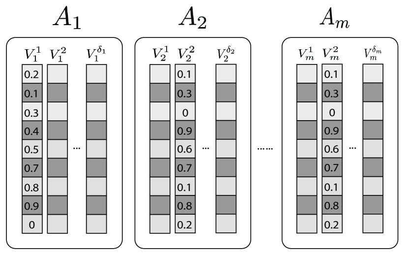
Figure 1: ${\sc DensityMap}$s

Example 1

The table in Figure 1 is stored over 9 blocks. The density map $D_{1}^{1}$ for $V_{1}^{1}$ is $\{0.2,0.1,0.3,0.4,0.5,0.7,0.8,0.9,0\}$, indicating 20 percent of tuples in block 1 and 10 percent of tuples in block 2 have value $V_{1}^{1}$ for attribute $A_{1}$ respectively.

DensityMaps are a very flexible index structure as they can estimate the percentage of valid records for any ad-hoc query with single or nested selection constraints. For queries with more than one predicate, we can combine multiple DensityMaps together to calculate the estimated percentage of valid records per block, multiplying densities for conjunction and adding them for disjunction. In performing this estimation, we implicitly assume that the DensityMaps are independent, akin to selectivity estimation in query optimization [25]. As in query optimization, this assumption may not always hold, but as we demonstrate in our experiments on real datasets, it still leads to effective results. In particular, DensityMaps drastically reduce the number of disk accesses by skipping blocks whose estimated densities are zero (and thus definitely do not contain valid records). Some readers may be reminded of other statistics used for query optimization, such as histograms [25]. However, unlike histograms which store the overall frequencies of records for entire relations, DensityMaps store this information at a finer block-level granularity.

Example 2

In Figure 1, for a given query Q with selection constraints $A_{1}$ = $V_{1}^{1}$ AND $A_{2}$ = $V_{2}^{2}$, the estimated DensityMap after combing $D_{1}^{1}$ and $D_{2}^{2}$ is $\{0.02,0.03,0,0.36,0.3,0.49,0.08,0.72,0\}$, indicating (approximately) that block 1 has 2 percent matching records, and block 2 has 3 percent matching records for Q.

Thus, compared to bitmaps, DensityMaps are a coarser statistical summary of valid records in each block for each attribute value. DensityMaps save significant storage costs by keeping information at the block-level instead of record-level, making maintaining DensityMaps in memory feasible. Moreover, coupled with efficient algorithms, which we describe in detail next, DensityMaps can decrease the number of blocks read from disk for any-$k$ sampling and therefore reduce the query execution time.

One concern with DensityMap is that, since we admit all records from a block which satisfy the constraints into our any-$k$ sample set, the samples we retrieve may be biased with respect to the data layout. In Section 6, we describe techniques to correct the bias due to possible correlations between the samples and the data layout by applying cluster sampling and unequal probability estimation techniques.

4 Any-K Algorithms: Extremes

We introduce two algorithms which take advantage of our DensityMaps to perform fast any-$k$ sampling. The primary insights for these algorithms come from the following two observations.

First, a high density block has more valid records than a low density block. Thus, it is more beneficial to retrieve the high density block, so that overall, fewer blocks are retrieved.

Observation 1 (Density: Denser is better.)

Under the same circumstances, retrieving a block with high density is preferable to retrieving a low density block.

In a HDD, the time taken to retrieve a block from disk can be split into seek time and transfer time. The seek time is the time it takes to locate the desired block, and the transfer time is the time required to actually transfer the bytes of data in the block from the HDD to the operating system. Blocks which are far apart incur additional seek time, while neighboring blocks typically only require transfer time. Thus, retrieving neighboring blocks is preferred. Similar locality arguments hold (to varying degrees) on SSD and RAM.

Observation 2 (Locality: Closer is better)

Under the same circumstances, retrieving neighboring blocks is preferable to retrieving blocks which are far apart.

Our basic any-$k$ sampling algorithms take advantage of each of these observations: Density-Optimal optimizes for density while Locality-Optimal optimizes for locality. These two algorithms are optimal extremes, favoring just one of locality or density.

On different types of storage media, the two observations can have different amounts of impact. For example, the locality observation may not be as important for in-memory data and solid-state drives (SSDs), since the random I/O performance of these storage media is not as poor as it is on HDDs. For our purposes, we focus on the HDDs, which is the most common type of storage device, but we also evaluate our techniques on SSDs.

To judge which of these two algorithms is better in a given setting, or to combine the benefits of these two algorithms, we require a cost model for storage media, which we present in Section 5.

Table 1 provides a summary of the notation used in the following sections.

Symbol	Meaning
$\lambda$	Number of blocks
$\gamma$	Number of predicates
$\tau$	Number of samples received
$\kappa$	An empirical constant to sequentially access one block
$S=\{S_{1},S_{2},\cdots,S_{\gamma}\}$	DensityMap indicated in the WHERE clause
$S_{j}[i]$	the $i$th entry of DensityMap $S_{j}$
$\hat{S}=\{\hat{S}_{1},\hat{S}_{2},\cdots,\hat{S}_{\gamma}\}$	Sorted DensityMap indicated in the WHERE clause
$\hat{S}_{i}[j]$	the $j$th entry of the $i$th sorted DensityMap in $\hat{S}$
$\theta$	Threshold
$M$	Set of block IDs with their aggregated densities
$Seen$	Set of block IDs seen so far
$R$	Set of block IDs returned by the algorithm

Table 1: Table of Notation

4.1 Density-Optimal Algorithm

Density-Optimal is based on the threshold algorithm proposed by Fagin et al. [23]. The goal of Density-Optimal is to use our in-memory DensityMap index to retrieve the densest blocks until $k$ valid records are found. The unmodified threshold algorithm by Fagin et al. would attempt to find the $p$ densest blocks. However, in our setting, we do not know the value of $p$ in advance: we only know $k$, the number of valid tuples required, so we need to set the value of $p$ on the fly.

For fast execution of Density-Optimal, an additional sorted DensityMap data structure is required. For every DensityMap $D$, we sort it in descending order of densities to create a sorted DensityMap $\hat{D}$. Every element $\hat{D}[i]$ has two attributes: $bid$, the block ID, and $density$, the percentage of tuples in this block which satisfies the corresponding constraint. Here $D[1]$ refers to the first block of the data and $\hat{D}[1]$ refers to the densest block in the data. Sorted DensityMaps are precomputed during data loading time and stored in memory along with the DensityMaps, so the sorting time does not affect the execution times of queries.

High-Level Intuition. At a high level, the algorithm examines each of the relevant sorted DensityMaps corresponding to the predicates in the query. It traverses these sorted DensityMaps in sorted order, while maintaining a record of the blocks with the highest overall density for the query, i.e., the highest number of valid tuples. The algorithm stops when the maintained blocks have at least $k$ valid records, and it is guaranteed that none of the unexplored blocks can have a higher overall density than the ones maintained.

Algorithmic Details. Algorithm 1 provides the full pseudocode. With sorted DensityMaps, it is easy to see how Density-Optimal handles a query with a single predicate: $A_{i}=V_{i}^{j}$. Density-Optimal simply selects the $\hat{D}_{i}^{j}$ which corresponds to the predicate and retrieves the first few blocks of $\hat{D}_{i}^{j}$ until $k$ valid records are found. For multiple predicates, the execution of Density-Optimal is more complicated. Depending on how the predicates are combined, $\bigoplus$ could mean $\prod$, i.e., product, if the predicates are all combined using ANDs, or $\sum$, i.e., sum, if the predicates are all combined using ORs. Each DensityMap in $\{S_{1},...,S_{\gamma}\}$ represents a predicate from the query, while $\{\hat{S}_{1},...,\hat{S}_{\gamma}\}$ represent the sorted variants. At each iteration, we traverse down $\hat{S}_{i}$, while maintaining a running threshold $\theta=\bigoplus_{j=1}^{\gamma}\hat{S}_{j}[i].density$, and also keeping track of all the block ids encountered across the sorted density maps. This threshold $\theta$ represents the minimum aggregate density that a block must have across the predicates before we are sure that it is one of the densest blocks. During iteration $i$, we consider all blocks in $M$ examined in the previous iterations that have not yet been selected to be part of the output. If the one with the highest density has density greater than $\theta$, then it is added to the output $R$. We know that $\theta$ is an upper-bound for any blocks that have not already been seen in this or the previous iterations, due to the monotonicity of the operator $\bigoplus$. Thus, Density-Optimal maintains the following invariant: a block is selected to be part of the output iff its density is as good or better than any of the blocks that not yet been selected to be part of the output. Overall, Density-Optimal ends up adding the blocks to the output in decreasing order of density. Density-Optimal terminates when the number of valid records in the output blocks selected is at least $k$.

To retrieve the any-$k$ samples, we then load the blocks returned by Density-Optimal into memory and return all valid records seen in those blocks. If the total number of query results in those blocks are less than $k$, we re-execute Density-Optimal on the blocks that have not been retrieved in previous invocations.

Fetch Optimization. Depending on the order of the blocks returned by Density-Optimal, the system may perform many unnecessary random I/O operations. For example, if Density-Optimal returns blocks $\{B_{100},B_{1},B_{83},B_{3}\}$, the system may read block $B_{100}$, seek to block $B_{1}$, and then seek back to block $B_{83}$, resulting in expensive disk seeks. Instead, we can sort the blocks $\{B_{1},B_{3},B_{83},B_{100}\}$ before fetching them from disk, thereby minimizing random I/O and overall query execution time.

Algorithm 1 Density-Optimal

1:Initialize $\theta\leftarrow 0$, $i\leftarrow 1$, $\tau\leftarrow 0$, $R,M,Seen\leftarrow\varnothing$

2:while $i\leq\lambda$ do

3:    $\theta\leftarrow\displaystyle\bigoplus_{j=1}^{\gamma}$ $\hat{S}_{j}[i].\textit{density}$

4:    for $j=1\dots\gamma$ do

5:         if $\hat{S}_{j}[i].bid\notin Seen$ then

6:             $\rho\leftarrow\hat{S}_{j}[i].bid$

7:             $\xi\leftarrow\left\{\begin{array}[]{ll}bid:&\rho\\ density:&\bigoplus_{k=1}^{\gamma}S_{k}[\rho].density\end{array}\right.$

8:             $M\leftarrow M\cup\{\xi\}$

9:             $Seen\leftarrow Seen\cup\{\rho\}$              

10:    $\mu\leftarrow\operatorname*{argmax}_{\mu^{\prime}\in M}\;\mu^{\prime}.density$

11:    while $\mu\geq\theta$  do

12:         $\tau\leftarrow\tau+\mu.density\times records\_per\_block$

13:         $R\leftarrow R\cup\{\mu.bid\}$

14:         $M\leftarrow M\setminus\{\mu\}$

15:         if $\tau\geq k$ then

16:             return $R$

17:         else

18:             $\mu\leftarrow\operatorname*{argmax}_{\mu^{\prime}\in M}\;\mu^{\prime}.density$              

19:    $i\leftarrow i+1$

20:return $R$

Guarantees. We now show that Density-Optimal retrieves the minimum set of blocks when optimizing for density.

Theorem 1 (Density Optimality)

Under the independence assumption, Density-Optimal returns the set of blocks with the highest densities with at least $k$ valid records.

Since Density-Optimal is a significant modification of the threshold algorithm the proof of the above theorem does not follow directly from prior work.

Proof 4.2.

The proof is composed of two parts: first, we demonstrate that Density-Optimal adds blocks to $R$ in the order of decreasing overall density; second, we demonstrate that Density-Optimal stops only when the number of valid records in $R$ is $\geq k$. The second part is obvious from the pseudocode (line 16). We focus on the first part. The first part is proven using an inductive argument. We assume that the blocks added to $R$ through $i$th iteration satisfy the property and that $\theta$ of the $i$th iteration is denoted as $\theta_{i}$. We note that for the $i+1$th iteration, $\theta_{i}\geq\theta_{i+1}$. Consider the blocks that are part of $M$ at the end of line 10 in the $i+1$th iteration. These blocks fall into two categories: either they were already part of $M$ in the $i$th iteration, and hence have densities less than $\theta_{i}$, or were added to $M$ in the $i+1$th iteration, and due to monotonicity, once again have density less than $\theta_{i}$. Furthermore, any blocks that have not yet been examined will have densities less than $\theta_{i+1}$. Since all blocks that have been added at iteration $i$ or prior have densities greater than or equal to $\theta_{i}$, all the blocks still under contention for adding to $R$—those in $M$ or those yet to be examined—have densities below those in $R$. Now, in iteration $i+1$, we add all blocks in $M$ whose densities are greater than $\theta_{i+1}$, in decreasing order. We know that all of these blocks have higher densities than all the blocks that have yet to be examined (once again using monotonicity). Thus, we have shown that any blocks added to $R$ in iteration $i+1$ are lower in terms of density than those added to $R$ previously, and are the best among the ones in $M$ and those that will be encountered in future iterations.

4.2 Locality-Optimal Algorithm

Our second algorithm, Locality-Optimal, prioritizes for locality rather than density, aiming to identify the shortest sequence of blocks that guarantee $k$ valid records. The naive approach to identify this would be to consider the sequence formed by every pair of blocks (along with all of the blocks in between)—leading to an algorithm that is quadratic in the number of blocks. Instead, Locality-Optimal, described below, is linear in the number of blocks.

High-level Intuition. Locality-Optimal moves across the sequence of blocks using a sliding window formed using a start and an end pointer, and eventually returns the smallest possible window with $k$ valid records. At each point, Locality-Optimal ensures that the window has at least $k$ valid records within it, by first advancing the end pointer until we meet the constraint, then advancing the start pointer until the constraint is once again violated. It can be shown that this approach considers all minimal sequences of blocks with $k$ valid records. Subsequently, Locality-Optimal returns the smallest such sequence.

Algorithmic Details. The pseudocode for the algorithm is listed in Algorithm 2. The Locality-Optimal algorithm operates on an array of values formed by applying the operator $\bigoplus$ to the predicate DensityMaps $\{S_{1},..,S_{\gamma}\}$, one block at a time. At the start, both pointers are at the value corresponding to the density of the first block. We move the end pointer to the right until the number of valid records between the two pointers is no less than $k$; at this point, we have our first candidate sequence containing at least $k$ valid records. We then move the start pointer to the right, checking if each sequence contains at least $k$ valid records, and continuing until the constraint of having at least $k$ valid records is once again violated. Afterwards, we once again operate on the end pointer. At all times, we maintain the smallest sequence found so far, replacing it when we find a new sequence that is smaller.

Algorithm 2 Locality-Optimal

1:Initialize $\tau\leftarrow 0$, $R\leftarrow\varnothing$

2:Initialize $start,end,min\_start,min\_end\leftarrow 1$

3:for $i=1\dots\lambda$ do

4:    $M[i]\leftarrow\left\{\begin{array}[]{ll}bid:&i\\ density:&\bigoplus_{j=1}^{\gamma}S_{j}[i].density\end{array}\right.$

5:while $end<\lambda$ do

6:    while $\tau<k$ and $end<\lambda$ do

7:         $\tau$ $\leftarrow\tau+M[end].density\times records\_per\_block$

8:         $end\leftarrow end+1$     

9:    while $\tau\geq k$ and $start<\lambda$ do

10:         if $(end-start)<(min\_end-min\_start)$ then

11:             $min\_end\leftarrow end$

12:             $min\_start\leftarrow start$          

13:         $\tau\leftarrow\tau-M[start].density\times records\_per\_block$

14:         $start\leftarrow start+1$     

15:$R\leftarrow\bigcup_{min\_start\leq i<min\_end}\{i\}$

16:return $R$

Guarantees. We now show that Locality-Optimal retrieves the minimum sequence of blocks when optimizing for locality.

Theorem 4.3 (Locality Optimality).

Under the independence assumption, Locality-Optimal returns the smallest sequence of blocks that contains at least $k$ valid records.

We demonstrate that for every block $i$, Locality-Optimal considers the smallest sequence of blocks with $k$ valid records beginning at block $i$ at some point in the algorithm, thereby proving the above theorem.

Proof 4.4.

For $i=1$, this is easy to see. The end pointer of Locality-Optimal starts at 1 and increases; the start pointer is not moved until a valid sequence of blocks is found, so by construction Locality-Optimal considers the smallest sequence of blocks starting at 1. For the remaining $i$’s we prove this by contradiction. Let the smallest sequence of blocks beginning at block $i$ end at $j$, where $j\geq i$; we denote this sequence as $[i,j]$. Now, let $j^{\prime}$ be the ending block for the smallest sequence of blocks starting at $i+1$; this sequence is denoted as $[i+1,j^{\prime}]$. If $j^{\prime}\geq j$, our Locality-Optimal algorithm considers the sequence as we move the end pointer forward (lines 6-8 in the pseudocode). Assume to the contrary that $j^{\prime}=j-1<j$; that is, the sequence $[i+1,j-1]$ is the smallest sequence of blocks starting at $i+1$ that has $k$ valid records. $[i+1,j-1]$ is a subsequence of $[i,j-1]$, so $[i,j-1]$ must also have at least $k$ valid records. However, we already declared $[i,j]$ to be the smallest sequence of blocks starting at $i$ that has $k$ valid records, and thus a contradiction is found. Similar arguments can be made for all $j^{\prime}<j-1$, so Locality-Optimal must consider the smallest sequence of blocks starting at block $i$ for every $i$.

5 Hybrid ANY-K Algorithms

The two desired properties of density and locality can often be at odds with each other depending on the data layout; dense blocks may be far apart, and neighboring blocks may contain many blocks which have no valid records. In this section, we first present a cost model to estimate the I/O cost of a any-$k$ algorithm, and use it to design an any-$k$ algorithm that is I/O-optimal, providing the best balance between density and locality, and a hybrid algorithm, that selects between Density-Optimal and Locality-Optimal.

5.1 A Simple I/O Cost Model

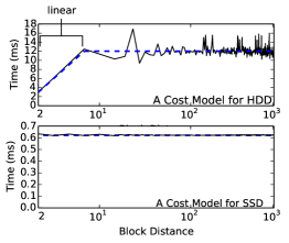
Figure 2: I/O Cost Model for HDDs and SSDs

To set up the cost model for I/O for HDDs (Hard Disk Drives), we profile the storage system as described by Ruemmler et al. [47]. We randomly choose various starting blocks and record the time taken to fetch other blocks that are varying distances away (where distance is measured in number of blocks), for distance onwards. As shown in Figure 2, which uses a linear scale on the x-axis from x=2 until x=10, and then logarithmic scale after that, we observe that with block size equal to 256KB, the I/O cost is smallest when doing a sequential I/O operation to fetch the next block ($\sim$ 2ms), and increases with the distance up to a certain maximum distance $t$ after which it becomes constant ($\sim$ 12ms). We have overlaid our cost model estimate using a dashed blue line. More formally, for two blocks $i$ and $j$, we model the cost of fetching block $j$ after block $i$ as follows:

$$RandIO(i,j)=\left\{\begin{array}[]{@{}c@{\quad}l@{}}cost(i,j)&\text{if $\left|j-i\right|\leq t$}\\ constant&\text{$otherwise$}\\ \end{array}\right.\vspace{-3pt}w$$

When distance is less than $t$, we use a simple linear fit for $cost(i,j)$, using the Python numpy.polyfit function

On the other hand, as shown in Figure 2, the I/O Cost Model for SSDs is different from the one we see for HDDs. Overall, we see a constant time ($\sim$ 0.6ms) to fetch a block (overlaid in a dashed blue line) independent of the block distance.

5.2 IO-Optimal Algorithm

IO-Optimal considers both density and locality to search for the set of blocks that will provide the minimum I/O cost overall. Specifically, given our cost model, we can use dynamic programming to find the optimal set of blocks with $k$ valid records.

We define $C(s,i)$ as the minimal cost to retrieve $s$ estimated valid records when block $i$ is amongst the blocks fetched. We define $Opt(s,i)$ as the cost to retrieve the optimal set of blocks with $s$ estimated valid records when considering the first $i$ blocks. Finally, we denote $s_{i}$ as the estimated number of valid records inside block $i$, derived, as before, using the $\bigoplus$ computation. With this notation, we have:

$$\small C(s,i) =\min\left\{\begin{array}[]{lr}C(s-s_{i},j)+RandIO(j,i),\quad\forall j\in[\,i-t,i-1]\\ Opt(s-s_{i},i-t-1)+RandIO(i-t-1,i)&\end{array}\right.$$

$$Opt(s,i) =\min\left\{\begin{array}[]{lr}C(s,i)\\ Opt(s,i-1)\end{array}\right.$$

The intuition is as follows: for each block $i$ that has $s_{i}$ estimated valid records, either the block can be in the final optimal set or not. If we decide to include block $i$, the cost is the minimum cost amongst the following: (i) the smallest I/O cost of having $s-s_{i}$ samples at block $j$ where $|i-j|\leq t$, plus the cost of jumping from block $j$ to $i$ (i.e., $C(s-s_{i},j)+RandIO(j,i)$), or (ii) the optimal cost at block $i-t-1$, plus the random I/O cost of jumping from some block in the first $i-t-1$ blocks to block $i$ (i.e., $Opt(s-s_{i},i-t-1)+RandIO(i-t-1,i))$.

For the second expression, if we exclude block $i$, then the optimal cost is the same as the optimal cost at block $i-1$. Consequently, the optimal cost at block $i$ is the smallest value in these two cases. The full algorithm is shown in Algorithm  3, where $\kappa$ is some constant cost to fetch the first block.

Algorithm 3 IO-Optimal

1:Initialize $R\leftarrow\varnothing$.

2:for $i=1\dots\lambda$ do

3:    $M[i]\leftarrow\left\{\begin{array}[]{ll}bid:&i\\ density:&\bigoplus_{j=1}^{\gamma}S_{j}[i].density\end{array}\right.$

4:    $s_{i}$ $\leftarrow$ $M[i].density\times records\_per\_block$

5:for $s$ = $0$ …$s_{1}$ do

6:    $C(s,1)\leftarrow\kappa$

7:    $Opt(s,1)\leftarrow\kappa$

8:for $s$ = $s_{1}+1,$ …$,k$ do

9:    $C(s,1)\leftarrow\infty$

10:    $Opt(s,1)\leftarrow\infty$

11:for $i$ = $2$ …$\lambda$ do

12:    for $s$ = $0$ …$s_{i}$ do

13:         $C(s,i)\leftarrow RandIO(1,i)$

14:         $Opt(s,i)\leftarrow\min{\{Opt(s,i-1),C(s,i)\}}$     

15:    for $j$ = $s_{i}+1,$ …$,k$ do

16:         $C(s,i)\leftarrow\min\left\{\begin{array}[]{lr}C(s-s_{i},j)+RandIO(j,i),\forall j\in[\,i-t,i-1]\\ Opt(s-s_{i},i-t-1)+RandIO(i-t-1,i)&\end{array}\right.$

17:         $Opt(s,i)\leftarrow\min{\{Opt(s,i-1),C(s,i)\}}$     

18:$R\leftarrow$ sequence of blocks that result the cost in $Opt(k,\lambda)$

19:return $R$

Guarantees. We can show the following property.

Theorem 5.5 (IO-Optimal).

Under the independence assumption and the constructed cost model for disk I/O, IO-Optimal gives the blocks with optimal I/O cost for fetching any-$k$ valid records.

The proof is listed in full detail in Appendix A.1.

5.3 Hybrid Algorithm

Even though IO-Optimal is able to return the optimal I/O cost for fetching any-$k$ samples, its much higher computation cost (as we show in our experiments) makes it impractical for large datasets. We propose Hybrid which simply selects between the best of Density-Optimal and Locality-Optimal, using our I/O cost model, when a query is issued. Since Hybrid needs to run both algorithms to determine the set of blocks selected by each algorithm, using Hybrid would involve a higher up-front computational cost, but as we will see, leads to substantial performance benefits.

6 Aggregate Estimation

So far, our any-$k$ algorithms retrieve $k$ records without any consideration of how representative they are of the entire population of valid records. If these records are used to estimate an aggregate (e.g., a mean), there could be bias in this value due to possible correlations between the value and the data layout. While this is fine for browsing, it leaves the user unable to make any statistically significant claims about the aggregated value. To address this problem, we make two simple adjustments to extend our any-$k$ algorithms. First, we introduce a Two-Phase sampling scheme where we add small amounts of random data to our any-$k$ estimates. This random data is added in a fashion such that it does not significantly affect the overall running time, while at the same time, allowing us to “correct for” the bias easily. Second, we correct the bias by leveraging techniques from the survey sampling literature. Specifically, we leverage the Horvitz-Thompson [31] and ratio [42] estimators, as described below. Note that such approaches have been employed in other settings in approximate query processing [44, 41, 21, 32, 36], but their application to any-$k$ is new.

6.1 Two-Phase Sampling

We propose a Two-Phase sampling scheme, in which we collect a large portion of the $k$ requested samples using an any-$k$ algorithm, and collect the rest in a random fashion. We denote $(1-\alpha)$ as the proportion of $k$ samples we retrieve using the any-$k$ algorithm, and $\alpha$ as the proportion of $k$ samples we retrieve using random sampling. The user chooses the parameter $\alpha$ upfront based on how much random sampling they wish to add. While a larger $\alpha$ may reduce the number of total samples needed to obtain a statistically significant result, the time taken to retrieve random samples greatly exceeds the time taken to retrieve samples based on our any-$k$ algorithms. Therefore, $\alpha$ needs to be carefully chosen; we experiment with different $\alpha$s in Section 9.

More formally, if we let $S_{v}$ be the set of blocks which have at least one valid record in them, we can describe Two-Phase sampling as follows: (1) Use an any-$k$ algorithm to choose the densest blocks $S_{c}$ from $S_{v}$, and derive $(1-\alpha)k$ samples from $S_{c}$. (2) Uniformly randomly select blocks $S_{r}$ from the remaining blocks, and derive $\alpha$ samples from $S_{r}$. Note that $S_{c}\cap S_{r}=\varnothing$.

6.2 Unequal Probability Estimation

Within the Two-Phase sampling scheme, the probability a block is sampled is not uniform. Therefore, we must use an unequal probability estimator [56] and inversely weigh samples based on their selection probabilities. We introduce two different estimators for this: the Horvitz-Thompson estimator and the ratio estimator.

6.2.1 Requisite Notation

The goal of our two estimators is to estimate the true aggregate sum $\tau$ and the true aggregate mean $\mu$ of measure attribute $M$ given a query $Q$. We use $\tau_{i}$ to denote the aggregate sum of $M$ for block $i$ and $L$ for the total number of valid records for query $Q$. We can estimate $L$ using the DensityMaps.

The estimators inversely weigh samples based on their probability of selection. So, we define the inclusion probability $\pi_{i}$ as the probability that block $i$ is included in the overall sample:

$$\pi_{i}=\begin{cases}1&\text{if }i\in S_{c}\\ \frac{|S_{r}|}{|S_{v}|-|S_{c}|}&\text{if }i\in S_{v}\setminus S_{c}\\ 0&\text{otherwise}\end{cases}$$

For the $(1-\alpha)k$ samples that come from the any-$k$ blocks in $S_{c}$, the probability of being chosen is always 1. After these blocks have been selected, a uniformly random subset of the remaining blocks are chosen to produce the $\alpha k$ random samples; thus the probability that these samples are chosen is $\frac{|S_{r}|}{|S_{v}|-|S_{c}|}$.

We define the joint inclusion probability $\pi_{ij}$ as the probability of selecting both blocks $i$ and $j$ for the overall sample:

$$\pi_{ij}=\begin{cases}1&\text{if }i\in S_{c}\land j\in S_{c}\\ \frac{|S_{r}|}{|S_{v}|-|S_{c}|}&\text{if }(i\in S_{c}\land j\in S_{r})\lor(i\in S_{r}\land j\in S_{c})\\ \frac{|S_{r}|}{|S_{v}|-|S_{c}|}\frac{|S_{r}|-1}{|S_{v}|-|S_{c}|-1}&\text{if }i\in S_{r}\land j\in S_{r}\\ 0&\text{otherwise}\end{cases}$$

6.2.2 Horvitz-Thompson Estimator

Using the Horvitz-Thompson [31] estimator, $\tau$ is estimated as:

$$\hat{\tau}_{HT}=\sum_{i\in S_{c}}\frac{\tau_{i}}{\pi_{i}}+\sum_{i\in S_{r}}\frac{\tau_{i}}{\pi_{i}}$$ (1)

As mentioned before, the sums $\tau_{i}$ are inversely weighted by their probabilities $\pi_{i}$ to account for the different probabilities of selecting blocks in $S_{v}$. Based on $\hat{\tau}_{HT}$, we can also easily estimate $\mu$ by dividing the size of the population:

$$\hat{\mu}_{HT}=\frac{\hat{\tau}_{HT}}{L}$$ (2)

The Horvitz-Thompson estimator guarantees us that both $\hat{\tau}_{HT}$ and $\hat{\mu}_{HT}$ are unbiased estimates: $E(\hat{\tau}_{HT})=\tau$ and $E(\hat{\mu}_{HT})=\mu$. A full proof can be found in [31]. In addition, the Horvitz-Thompson estimator gives us a way to calculate the variances of of $\hat{\tau}_{HT}$ and $\hat{\mu}_{HT}$, which represent the expected bounds of $\hat{\tau}_{HT}$ and $\hat{\mu}_{HT}$:

$$Var({\hat{\tau}_{HT}})=\sum_{i\in S_{v}}\left(\frac{1-\pi_{i}}{\pi_{i}}\right)\tau_{i}^{2}+\sum_{i\in S_{v}}\sum_{j\neq i}\left(\frac{\pi_{ij}-\pi_{i}\pi_{j}}{\pi_{i}\pi_{j}}\right)\tau_{i}\tau_{j}$$ (3)

$$Var(\hat{\mu}_{HT})=Var(\hat{\tau}_{HT}/L)=Var(\hat{\tau}_{HT})/L^{2}$$ (4)

6.2.3 Ratio Estimator

Although the Horvitz-Thompson estimator is an unbiased estimator, it is possible that the variances given by Equations 3 and 4 can be quite large if the aggregated variable is not well related to the inclusion probabilities [56]. To reduce the variance, the ratio estimator [42] may be used:

$$\hat{\mu}_{R}=\frac{\hat{\tau}_{HT}}{\sum_{i\in S_{c}\cup S_{r}}\frac{L_{i}}{\pi_{i}}}$$ (5)

$$\hat{\tau}_{R}=\hat{\mu}_{R}L$$ (6)

where $L_{i}$ is the number of valid records in block $i$. The variances of $\hat{\mu}_{R}$ and $\hat{\tau}_{R}$ are given by:

$$Var(\hat{\mu}_{R})= \frac{1}{L^{2}}\Bigg{[}\sum_{i\in S_{v}}\left(\frac{1-\pi_{i}}{\pi_{i}}\right)(\tau_{i}-\mu)^{2}$$

$$+\sum_{i\in S_{v}}\sum_{j\neq i}\left(\frac{\pi_{ij}-\pi_{i}\pi_{j}}{\pi_{i}\pi_{j}}\right)(\tau_{i}-\mu)(\tau_{j}-\mu)\Bigg{]}$$ (7)

$$Var(\hat{\tau}_{R})=Var(\hat{\mu}_{R}L)=L^{2}Var(\hat{\mu}_{R})$$ (8)

While the ratio estimator is not precisely unbiased, in Equation 5, we see that the numerator is the unbiased Horvitz-Thompson estimate of the sum and the denominator is an unbiased Horvitz-Thompson estimate of the total number of valid records, so the bias tends to be small and decreases with increasing sample size.

We compare the empirical accuracies of these two estimators in Section 9, and demonstrate how our Two-Phase sampling technique, when employing these estimators, provides accurate estimates of various aggregates values.

7 Grouping and Joins

So far, we have assumed that all our sampling queries have the form dictated by the SELECT query given in Section 2, thus limiting our operations to a single database table, with simple selection predicates and no group-by operators. We now extend the any-$k$ sampling problem formulation and our algorithms to handle more complex queries that involve grouping and join operations.

7.1 Supporting Grouping

Rather than computing a simple any-$k$, users may want to retrieve $k$ values per group, e.g., to compute an estimate of an aggregate value in each group.

Although a trivial way to do this would be to run a separate any-$k$ query per group, in this section we discuss an algorithm that can share the computation across groups in the common case when users want $k$ values per group.

Consider an any-$k$ query $Q_{k}$ over a table $T$ with $S$ representing the predicate in the where clause. Let $A_{G}$ be the grouping attribute with values in $\{V_{G}^{1},V_{G}^{2},\ldots,V_{G}^{\delta_{G}}\}$. The formal goal of this grouped any-$k$ sampling can be stated as:

Problem 7.6 (grouped any-$k$ sampling).

Given a query $Q_{k}$ defined by a predicate S on table $T$, and a grouping attribute $A_{G}$, the goal of grouped any-$k$ sampling is to retrieve any $k$ valid records for each group in as little time as possible.

Our basic approach is to create a combined density map, which takes into account every group in the group-by operation, and run the any-$k$ algorithm for all groups at once. This is akin to sharing scans in traditional databases.

In order to run our any-$k$ algorithms for all groups, we first define the combined density of the $l$th block as multiplication of two factors: (1) the density of the $l$th block with respect to predicate $S$, and (2) the sum of the densities for group values in $A_{G}$ in the $l$th block which still need to be sampled. The first factor has been discussed previously, while the second factor can be defined as:

$$\vspace{-3pt}d_{G_{l}}^{*}=\frac{1}{\text{RPB}}\sum_{j=1}^{\delta_{G}}min\left(k-r_{G}^{j}\;,\;d_{G_{l}}^{j}\times\text{RPB}\right)\vspace{-3pt}$$ (9)

where RPB is $records\_per\_block$, $r_{G}^{j}$ is the number of samples already retrieved for group $V_{G}^{j}$, and $d_{G_{l}}^{j}$ is the density of the $l$th block for the value $V_{G}^{j}$. The expression inside the $min$ function estimates the number of expected records in block $l$ for each group $V_{G}^{j}$, but limits the estimate by the number of samples left to be retrieved for that group. Thus, the combined density ($d_{S_{l}}d_{G_{l}}^{*}$), where $d_{S_{l}}$ is the density of the $l$th block with respect to predicate $S$, gives priority to groups which have had fewer than k samples retrieved so far, and groups which already have $k$ samples no longer contribute to the combined density. The $1/$RPB in front of the summation for $d_{G_{l}}^{*}$ acts a normalization factor to ensure that $d_{G_{l}}^{*}$, and thereby $d_{S_{l}}d_{G_{l}}^{*}$, are both density values between 0 and 1.

With this combined density estimate $d_{S_{l}}d_{G_{l}}^{*}$, we can now construct an iterative any-$k$ algorithm for grouped sampling operations, similar to the algorithms in Sections 4 and 5. The main structure of the algorithm is as follows: (1) Update all densities using with $d_{S_{l}}d_{G_{l}}^{*}$. (2) Run one of the any-$k$ algorithms to retrieve $\psi$ blocks with the highest combined density. (3) Update the densities of the $\psi$ blocks as 0. (4) If $k$ samples still have not been retrieved for each group, go back to step (1). Since $d_{G_{l}}^{*}$ depends on the number of samples already retrieved, it must be updated periodically to ensure the correctness of the combined densities. The $\psi$ parameter controls the periodicity of these updates. The problem of setting $\psi$ becomes a trade-off between CPU time and I/O time. Setting $\psi=1$ updates the densities after every block retrieval; while this more correctly prioritizes blocks and is likely to lead to fewer blocks retrieved overall, there is a high CPU cost in updating the densities after each block retrieval. As $\psi$ increases, the CPU cost goes down due to less frequent updates, but the overall I/O cost is likely to go up since the combined densities are not completely up-to-date for each block retrieved. Although our iterative algorithm is not particularly complex, and globally IO-optimal solutions may perform better than our locally optimal solution, our algorithm has the advantage of simplicity of implementation and likely lower CPU overhead. We defer consideration of more sophisticated algorithms to future work.

Algorithm Details. The full algorithm for the grouping any-$k$ query is shown in Algorithm 4. In Section 4, $\tau$ was a single value representing the number of samples retrieved; for the grouping any-$k$ algorithm, $\tau$ is now an array of size $\delta_{G}$ where each entry represents the number of samples for that group. Every iteration consists of updating the combined density estimates or the priorities of blocks $M$ based on the number of samples retrieved (setting it to 0 if it has already been seen), and calling an any-$k$ algorithm with $M$ and the number of blocks desired $\psi$. The algorithm updates the counts of $\tau$ and the algorithm only ends once every entry in $\tau$ is at least $k$.

Algorithm 4 Group-by any-$k$ algorithm.

1:Initialize $\tau\leftarrow[0,...,0]$, $R,M\leftarrow\varnothing$

2:while $\exists j\in\{1,...,\delta_{G}\},\;\tau[j]<k$ do

3:    for $i=1\dots\lambda$ do

4:         if $i\in R$ then

5:             $M[i]\leftarrow\left\{\begin{array}[]{ll}bid:&i\\ density:&0\end{array}\right.$

6:         else

7:             $M[i]\leftarrow\left\{\begin{array}[]{ll}bid:&i\\ density:&d_{S_{i}}\sum_{j=1}^{\delta_{G}}d_{G_{i}}^{*}\end{array}\right.$              

8:    $R^{\prime}\leftarrow\text{any-$k$}(M,\psi)$

9:    for $r\in R^{\prime}$ do

10:         for $j\in\{1,...,\delta_{G}\}$ do

11:             $\tau[j]\leftarrow\tau[j]+d_{S_{r}}d_{G_{r}}^{j}\times records\_per\_block$              

12:    $R\leftarrow R\cup R^{\prime}$

13:return $R$

As we show in the next section, the key-foreign key join any-$k$ problem is essentially equivalent to this grouped any-$k$ formulation, and we evaluate the performance of our algorithm on these problems in Section 9.7.

Optimal Solution. As mentioned, the grouping any-$k$ solution uses a heuristic to find the best blocks to retrieve. However, an I/O optimal solution, similar to IO-Optimal from Section 5.2, could be derived using dynamic programming with a recursive relationship based on the notion of priority from Equation 9, $\tau$, and the disk model from Section 5.2. Unfortunately, the resulting dynamic programming solution becomes a complex program of even more dimensions than the program from Section 5.2. Since we already showed in Section 9 that IO-Optimal incurs a prohibitively high CPU cost in exchange for its optimal I/O time, we chose not to pursue this avenue.

Multiple Groupings. For multiple group-by attributes, we simply extend the above formula to account for every possible combination of values from the different groupings. For example, if we have two group-by attributes $A_{G}$ and $A_{G^{\prime}}$ , we can specify our updated notion of density with $d_{S_{l}}\sum_{j=1}^{\delta_{G}}\sum_{i=1}^{\delta_{G^{\prime}}}d_{G_{l}}^{*}d_{{G^{\prime}}_{l}}^{*}.$

7.2 Supporting Key-Foreign Key Joins

Consider any-$k$ sampling on the result of a key-foreign key join between two tables $T$ and $T^{\prime}$, where $A_{J}$ is the primary key in $T$, and $A_{J^{\prime}}$ is the foreign key in $T^{\prime}$. Similar to grouping, the formal definition of join any-$k$ sampling can be defined as:

Problem 7.7 (join any-$k$ sampling).

Given a query $Q_{k}$ defined by a predicate $S$ and a join over tables $T$ and $T^{\prime}$, on primary key $A_{J}$ from table $T$ and foreign key $A_{J^{\prime}}$ from table $T^{\prime}$, the goal of join any-$k$ sampling is to retrieve any $k$ valid joined records for each join value in as little time as possible.

For example, if we want to join on a “departments” attribute, $k$ samples would be retrieved for each department.

Since we assume $A_{J}$ is the primary key, and therefore unique, the join any-$k$ sampling problem can be reduced to finding any $k$ valid records in table $T^{\prime}$ for each join value $V_{J}\in A_{J}$. However, this is the exact same problem as the grouped any-$k$ sampling problem in which the group values are $V_{J}\in A_{J}$. Thus, we can use the algorithm described in the previous section, using the values of $A_{J}$ as the grouping value on the foreign key table $T^{\prime}$.

In this way, NeedleTail is able to best indicate the blocks that can be retrieved to minimize the overall time for joins. We evaluate our join any-$k$ algorithm in Section 9.7. We leave optimizations for other join variants as future work.

8 System Design

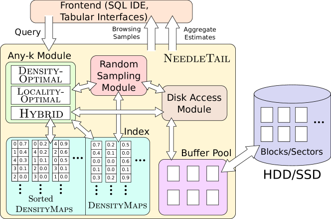
Figure 3: NeedleTail Architecture

We implemented our DensityMaps, any-$k$ algorithms, and aggregate estimators in a system called NeedleTail. NeedleTail is developed as a standalone browsing-based data exploration engine, capable of returning individual records as well as estimating aggregates. NeedleTail can be invoked by various frontends, e.g., SQL IDEs or interfaces such as Tableau or Excel. Figure 3 depicts the overall architecture of NeedleTail. It includes four major components: the any-$k$ module, the random sampling module, the index, and the disk access module. The any-$k$ module receives queries from the user and executes our any-$k$ algorithms from Sections 4, 5, and 7 to return any-$k$ browsing samples as quickly as possible. For aggregate queries, the random sampling module is used in conjunction with the any-$k$ module to perform the Two-Phase sampling from Section 6. The index contains the DensityMaps and sorted DensityMaps. Finally, the disk access module is in charge of interacting with the buffer pool to retrieve blocks from disk. Since DensityMaps are a lossy compression of the original bitmaps, it is possible that some blocks with no valid records may be returned; these blocks are filtered out by the disk access module.

Our NeedleTail prototype is currently implemented in C++ using about 5000 lines of code. It is capable of reading in row-oriented databases with int, float, and varchar types and supports Boolean-logic predicates. Although the current implementation is limited to a single machine, we plan to extend NeedleTail to run in a distributed environment in the future. We believe the collective memory space available in a distributed environment will allow us to leverage the DensityMaps in even better ways.

9 Performance Evaluation

In this section, we evaluate NeedleTail, focusing on runtime, memory consumption, and accuracy of estimates. We show that our DensityMap-based any-$k$ algorithms outperform any “first-to-$k$-samples” algorithms using traditional OLAP indexing structures such as bitmaps or compressed bitmaps on a variety of synthetic and real datasets. In addition, we empirically demonstrate that our Two-Phase sampling scheme is capable of achieving as accurate an aggregate estimation as random sampling in a fraction of the time. Then, we demonstrate that our join any-$k$ algorithms provide substantial speedups for key-foreign key joins. We conclude the section with an exploration into the effects of different parameters on our any-$k$ algorithms.

9.1 Experimental Settings

We now describe our experimental workload, the evaluated algorithms, and the experimental setup.

Synthetic Workload: We generated 10 clustered synthetic datasets using the data generation model described by Anh and Moffat [11]. Every synthetic dataset has 100 million records, 8 dimension attributes, and 2 measure attributes. For the sake of simplicity, we forced every dimension attribute to be binary (i.e., valid values were either 0 or 1), and with measure attributes being sampled from normal distributions, independent of the dimension attributes. For each dimension attribute, we enforced an overall density of 10%; the number of 1’s for any attribute was 10% of the overall number of records. Since we randomly generated the clusters of 1’s in each attribute value, we ran queries with equality-based predicates on the first two dimensional attributes (i.e., $A_{1}=0$ and $A_{2}=1$). Note that this does not always result in a selectivity of 10% since the records whose $A_{1}=0$ may not have $A_{2}=1$.

Real Workload: We also used two real datasets.

• Airline Dataset [1]: This dataset contained the details of all flights within the USA from 1987–2008, sorted based on time. It consisted of 123 million rows and 11 attributes with a total size of 11 GB. We ran 5 queries with 1 to 3 predicates on attributes such as origin airport, destination airport, flight-carrier, month, day of week. For our experiments on error (described later), we estimated the average arrival delay, average departure delay, and average elapsed time for flights.

• NYC Taxi Dataset [5]: This dataset contained logs for a variety of taxi companies in New York City for the years 2014 and 2015. The dataset as provided was first sorted by the year; within each year, it was first sorted on the three taxi types and then on time. It consisted of 253 million rows and 11 attributes with a total size of 21 GB. We ran 5 queries with 1 to 2 predicates on attributes including pickup location, dropoff location, time slots, month, passenger count, vendors, and taxi type. For our experiments on error, we estimated the average fare amount and average distance traveled for the chosen trips.

Algorithms: We evaluated the performance of the three any-$k$ algorithms presented in Section 4 and 5: (i) IO-Optimal, (ii) Density-Optimal, (iii) Locality-Optimal, and (iv) Hybrid We compared our algorithms against the following four “first-to-$k$-samples” baselines. Bitmap-Scan and Disk-Scan are representative of how current databases implement the LIMIT clause.

• Bitmap-Scan: Assuming we have bitmaps for every predicate, we use bitwise AND and OR operations to construct a resultant bitmap corresponding to the valid records. We then retrieve the first $k$ records whose bits are set in this bitmap.

• Lossy-Bitmap [62]: Lossy-Bitmap is a variant of bitmap indexes where a bit is set for each block instead of each record. For each attribute value, a set bit for a block indicates that at least one record in that block has that attribute value. During data retrieval, we perform bitwise AND or OR operations and on these bitmaps then fetch $k$ records from the first few blocks which their bit set. Note that this is equivalent to a DensityMap which rounds its densities up to 1 if it is $>0$.

• EWAH: This baseline is identical to Bitmap-Scan, except the bitmaps are compressed using the Enhanced Word-Aligned Hybrid (EWAH) technique [40] implemented using  [3]

• Disk-Scan: Without using any index structures, we continuously scan the data on disk until we retrieve $k$ valid records.

For our experiments on aggregate estimation, we compared our Two-Phase sampling algorithms against the baseline Bitmap-Random, which is similar to Bitmap-Scan, except that it selects $k$ random records among all the valid records. We describe our setup for the join any-$k$ experiments in Section 9.7.

Figure 4: Query runtimes for the synthetic workload on a HDD.

Setup: All experiments were conducted on a 64-bit Linux server with 8 3.40GHz Intel Xeon E3-1240 4-core processors and 8GB of 1600 MHz DDR3 main memory. We tested our algorithms with a 7200rpm 1TB HDD and a 350GB SSD. For each experimental setting, we ran 5 trials (30 trials for the random sampling experiments) for each query on each dataset. In every trial, we measured the end-to-end runtime, the CPU time, the I/O time, and the memory consumption. Before each trial, we dropped the operating system page cache and filled it with dummy blocks to ensure the algorithms did not leverage any hidden benefits from the page cache. To minimize experimental variance, we discarded the trials with the maximum and minimum runtime and reported the average of the remaining. Finally, after empirically testing a few different block sizes, we found 256KB to be a good default block size for our datasets: the block size does not significantly impact the relative performance of the algorithms.

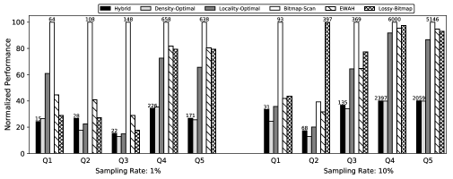
Figure 5: Query runtimes for airline workload on a HDD.

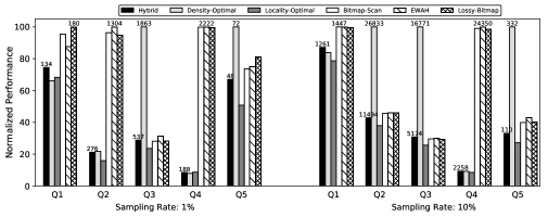
Figure 6: Query runtimes for taxi workload on a HDD.

9.2 Query Execution Time

Summary: In the synthetic datasets on a HDD, our Hybrid any-$k$ sampling algorithm was on average 13$\times$ faster than the baselines. For the real datasets, Hybrid performed at least as well as the baselines for every query, and on average was 4$\times$ and 9$\times$ faster for queries on HDDs and SSDs respectively.

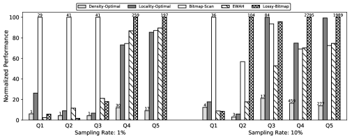
Figure 7: Query runtimes for airline workload on a SSD.

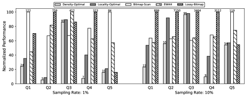
Figure 8: Query runtimes for taxi workload on a SSD.

Synthetic Experiments on a HDD. Figure 4 presents the runtimes for Hybrid, Density-Optimal, Locality-Optimal, and the four baselines for varying sampling rates. (We will evaluate IO-Optimal later on.) Sampling rate is defined to be the ratio of $k$ divided by the number of valid records. Since the queries can have a wide variety in the number of valid records, we decided to plot the impact on varying sampling rate rather than $k$. (Results for varying $k$ are similar.) The bars in the figure above represent the average runtimes for five sampling rates over 10 synthetic datasets. Note that the figure is in log-scale.

Regardless of the sampling rate, Density-Optimal, Hybrid, and Locality-Optimal significantly outperformed Bitmap-Scan, Lossy-Bitmap, EWAH, and Disk-Scan, with speedups of an order of magnitude. For example, for a sampling rate of 1%, Density-Optimal, Locality-Optimal, and Hybrid took 74ms, 45ms, and 58ms on average respectively, while Bitmap-Scan, Lossy-Bitmap, EWAH, and Disk-Scan took 647ms, 624ms, 662ms and 630ms on average respectively. Thus, our any-$k$ algorithms are more effective at identifying the right sequence of blocks that contain valid records than the baselines which do not optimize for any-$k$—the baselines are subject to the vicissitudes of random chance: if there are large number of valid records early on, then they will do well, and not otherwise. This is despite the fact that Bitmap-Scan and EWAH store more fine-grained information than our algorithms, and are therefore able to effectively skip over blocks without valid records.

There was no consistent winner between Density-Optimal and Locality-Optimal across sampling rates and queries, but Hybrid always selected the faster algorithm from the two and thus had an average speedup of 13$\times$ over the baselines. Despite that, Hybrid’s performance on lower sampling rates (0.1%, 1%) is a bit worse than Density-Optimal and Locality-Optimal, since it has to run both algorithms and pick the better one: but this difference in performance is small—around 10ms. From 5% onwards, Hybrid’s performance is clearly better than Density-Optimal and Locality-Optimal, since the increase in computation time is dwarfed by the improvement in I/O time.

Real Data Experiments on a HDD. Figures 5 and 6 show the runtimes of our algorithms over 5 diverse queries for the airline and taxi workloads respectively. For each query and sampling rate, we normalized the runtime of each algorithm by the largest runtime across all algorithms, while also reporting actual runtime (in ms) taken by Hybrid and the maximum runtime. We omitted Disk-Scan since Disk-Scan was found to be have the worst runtime in the previous experiment, and similarly performs poorly here. For the real workloads, we noticed that the runtimes of the queries were much more varied, so we report the average runtime for each query separately.

For the airline workload, we noticed that our any-$k$ algorithms consistently outperformed the bitmap-based baselines: Density-Optimal had a speedup of up to 8 compared to Bitmap-Scan and EWAH, while Locality-Optimal had a speedup of up to 7$\times$. Across all queries, when sampling rate equals 1%, Density-Optimal and Locality-Optimal were on average 3$\times$ and 5$\times$ faster than Bitmap-Scan and EWAH, despite having a much smaller memory footprint (Section 9.3). For example for Q3, which had two predicates on month and origin airport, the block with the highest density contained 1% samples already. Moreover, since the airline dataset is naturally sorted on time attributes (e.g., year, month), the valid tuples were more likely to clustered in a few number of blocks. Therefore, compared with Locality-Optimal, Density-Optimal fetched up to 10% less blocks, resulting in less query execution time than Locality-Optimal in all of cases. For the small additional cost of estimating the sequence of blocks for both Locality-Optimal and Density-Optimal, Hybrid ends up always selecting the faster algorithm in both this and the taxi workload, with an average speedup of 4$\times$. For example, for Q4 with 1% sampling rate Hybrid’s time is closer to Density-Optimal, and half of that of Locality-Optimal.

We noticed a different (and somewhat surprising) trend for the taxi workload. Here, Hybrid continued to do well, and much better than the worst algorithm on every setting, with an average speedup of 4$\times$ compared to the baselines. Similarly, Locality-Optimal performed similar or better than the baselines for every experiment. However, on multiple occasions, we found that Density-Optimal was slower than the baselines, and was the worst algorithm, e.g., in Q3 and Q5. Upon closer examination, we found that Density-Optimal did in fact retrieve the fewest number of blocks for every query. However, the taxi dataset was much larger than the airline dataset, so the blocks were more spread out, and the time to seek from block to block went up significantly. As a result, we found the locality-favoring Locality-Optimal to perform better on a HDD where seeks were expensive. To further exacerbate the issue, we found that the taxi workload also had a much more uniform distribution of tuples; the tuples that satisfied query predicates (which were not based on taxi type) were spread fairly uniformly across the dataset. In some sense, this made the dataset “adversarial” for density-based schemes. In other words, it is hard to conclude either Density-Optimal or Locality-Optimal is better than another, given their performance depends on the distribution of valid tuples of a given ad-hoc query—and it is therefore safer to use Hybrid to pick between the two.

Real Data Experiments on a SSD. We also ran the same workload on SSD; SSDs have random I/O performance that is comparable to sequential I/O performance. The results are depicted in Figures 7 and 8. We omit Hybrid, since Hybrid always selects Density-Optimal over Locality-Optimal due to the fact that Density-Optimal fetches the smallest number of blocks. Overall, the performance of Density-Optimal is much faster than the bitmap-based baselines, with average speedups of 14$\times$ and 6$\times$ in the airline and taxi workload respectively. There were two exceptions: Q1 (10%) in airline and Q3 in taxi, where the total number of blocks fetched by Density-Optimal, Bitmap-Scan, Lossy-Bitmap, and EWAH were similar. In this uncommon situation, even though Density-Optimal has the lowest I/O time, the CPU cost of checking for valid records in each block was slightly higher, thus its runtime was a little higher than Bitmap-Scan and EWAH.

9.3 Memory Consumption

Summary: DensityMaps consumed on average 48$\times$ less memory than the regular bitmaps and 23$\times$ less memory than EWAH-compressed bitmaps.

Dataset	Disk Usage	# Tuples	Cardinality	Bitmap	EWAH	LossyBitmap	DensityMap
Synthetic	7.5 GB	100M	16	190.73MB	182.74MB	0.06MB	3.73MB
Taxi	21 GB	253M	64	1936.99MB	663.63MB	0.65MB	41.63MB
Airline	11GB	123M	805	11852.33MB	744.05MB	3.98MB	254.72MB

Table 2: Memory consumption of index structures.

Table 2 reports the amount of memory used by DensityMaps compared to the other three bitmap baselines. We observed that DensityMaps were very lightweight and consumed around 51$\times$, 47$\times$, and 47$\times$ less memory than uncompressed bitmaps respectively in the three datasets. Even with EWAH-compression, we observed an almost 49$\times$ reduction in size for the taxi dataset for DensityMaps relative to EWAH. In the airline dataset, since the selectivity of each attribute value is low, EWAH compressed the bitmaps much better than in the other two datasets. Still, EWAH consumed 3$\times$ more memory than DensityMap. Lastly, since Lossy-Bitmap requires only one bit per block while DensityMap is represented as a 64-bits double per block respectively, Lossy-Bitmap unsurprisingly consumed less memory than DensityMap. However, as we showed in Section 9.2, the smaller memory consumption incurred a large cost in query latency due to the large number of false positives (e.g., Q3 with sampling rate 10% in Figure5); especially when the number of predicates is large and exhibit complex correlations. In comparison, the DensityMap-based any-$k$ algorithms were orders of magnitude faster than the baselines, while still maintaining a modest memory footprint ($\sim 0.1\%$ of original dataset).

9.4 IO-Optimal Performance

Summary: IO-Optimal had up to 3.9$\times$ faster I/O time than Hybrid and the best I/O performance among all the algorithms described above. However, its large computational cost made it impractical for real datasets.

For the evaluation of IO-Optimal, we used a smaller synthetic dataset of 1 million records and a block size of 4KB, and conducted the evaluation on a HDD. We compared its overall end-to-end runtime, CPU time, and I/O time with every other algorithm, and found that it consistently had the best I/O times. However, we found that computational cost of dynamic programming in IO-Optimal outweighed any benefits from the shorter I/O time. Consequently, we found IO-Optimal to be impractical for larger datasets. Figure 9 shows both the overall times and I/O times for IO-Optimal and Hybrid for varying sampling rates.

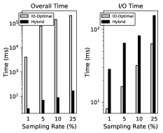
Figure 9: Overall and I/O time for IO-Optimal and Hybrid.

9.5 Time vs Error Analysis

Summary: Compared to random sampling using bitmap indexes, our Two-Phase sampling schemes that mix samples from any-$k$ sampling algorithms with a small percentage of random cluster samples attained the same error rate in much less time.

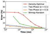
(a) NYC-Taxi - Ratio Estimator

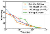
(b) Airline - Ratio Estimator

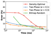
(c) NYC-Taxi - HT Estimator

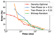
(d) Airline - HT Estimator

Figure 10: Time vs empirical error.

Using the Two-Phase sampling techniques in Section 6, we can obtain estimates of aggregate values on data; here we experiment with $\alpha=0\%,10\%,30\%$ random samples, and use the Density-Optimal algorithm, since it ended up performing the most consistently well across queries and workloads, for SSDs and HDDs. We compared these results with pure random sampling (Bitmap-Random) using bitmaps on a HDD. We used the same set of queries as in Section 9.2. For each query, we varied the sampling rate and measured the runtime and the empirical error of the estimated aggregate with respect to the true average value. Figure 10 depicts the average results for both the Horvitz-Thompson estimator and the ratio estimator. In log scale. We’ll start with the taxi dataset and the ratio estimator. Figure 10a shows that if all the sampling schemes are allowed to run for 500ms (commonly regarded as the threshold for interactivity), Density-Optimal, Two-Phase sampling with $\alpha=0.1$, Two-Phase sampling with $\alpha=0.3$, and Bitmap-Random have average empirical error rates of 29.64%, 4.83%, 3.66% and 19.64%, respectively; the corresponding number of the samples retrieved are 11102, 7977, 5684, 35 respectively. Thus, the Two-Phase sampling schemes are able to effectively correct the bias in Density-Optimal, while still retrieving a comparable amount of samples. Furthermore, note that Bitmap-Random suffers from the same problem as Bitmap-Scan in large memory consumption. In contrast, even though Density-Optimal was not the fastest algorithm in the taxi workload, our Two-Phase sampling algorithms cluster sample at the block level and only need access to the much more compressed DensityMaps.

The behavior on the airline workload is somewhat different: here we find that Density-Optimal performs better than the Two-Phase sampling scheme with the ratio estimator for the initial period until about 100ms, after which the Two-Phase sampling schemes perform better than Density-Optimal and Bitmap-Scan. We found this behavior repeated across other queries and trials: Density-Optimal sometimes ends up having very low error (like in Figure 10b), and sometimes fairly high error (like in Figure 10a), but the Two-Phase sampling schemes consistently achieve low error relative to Density-Optimal. This is because Density-Optimal’s accuracy is highly dependent on the correlation between the data layout and the attribute of interest, and can sometimes lead to highly biased results. At the same time, the Two-Phase sampling schemes return much more samples and much more accurate estimates than Bitmap-Random, effectively supporting browsing and sampling at the same time.

Between the Horvitz-Thompson estimator and the ratio estimator, the ratio estimator often had higher accuracies. As explained in Section 6, the ratio estimator works quite well in situations where aggregation estimate is not correlated with the block densities. We found this to be the case for both the airline and taxi workloads, so the ratio estimator helped for both these workloads.

9.6 Effect of Parameters

To explore the properties of our any-$k$ algorithms, we varied various parameters and noted their effect on overall runtimes for synthetic workloads. Varied parameters included: (i) data size, (ii) number of predicates, (iii) density, (iv) block size, and (v) granularity.

Data Size: We varied the synthetic dataset size from 1 million to 1 billion, but we found that the overall runtimes of our any-$k$ algorithms remained relatively the same. Our algorithms return only a fixed $k$ number of samples and explicitly avoid reading the entire dataset, so it makes sense that the runtimes stay consistent even when the data size increases.

Number of Predicates: As we increased the number of predicates in a query, we saw that overall runtimes increase as well. Since our predicates were combined using ANDs, an increase in the number of predicates meant a decrease in the number of valid records per block. Therefore, both Density-Optimal and Locality-Optimal needed to fetch more blocks to retrieve the same number of samples, and this caused an increase in the overall runtime.

Density: As we increased the overall density of valid records in the dataset, the runtimes for our any-$k$ algorithms got faster. As the overall density increased, the average density per block also increased, so our any-$k$ algorithms could retrieve fewer blocks to achieve the same number of $k$ samples.

Block Size: We tried varying the block sizes of our datasets from 4KB, to 256KB, to 1MB, to 2MB. We found that as we decreased the block sizes, the runtimes for Density-Optimal increased drastically because smaller block sizes meant that more random I/O was being done. However, we did not see any definite correlation as we increased the block size. Although larger block sizes do bias the algorithms toward more locality, they also mean density information is collected at a coarser granularity. We suspect that this tradeoff prevented us from seeing any improvements in performance with increased block size.

9.7 Key-Foreign Key Join Performance

Sampling Rate	Shared-Scan	Bitmap-Combined	Density-Combined ($\Psi$=5)	Density-Combined ($\Psi$=10)	Density-Combined ($\Psi$=50)
0.1%	2465.67	215.678	67.6398	63.7114	73.7204
0.5%	2632.32	1049.92	307.534	300.023	301.193
1.0%	2761.74	1424.12	616.090	593.258	591.201

Table 3: Query runtimes (in ms) on SSD for join operations on foreign key tables with 10 million rows.

Sampling Rate	Shared-Scan	Bitmap-Combined	Density-Combined ($\Psi$=5)	Density-Combined ($\Psi$=10)	Density-Combined ($\Psi$=50)
0.1%	1266.06	110.63	33.59	32.38	68.16
0.5%	1359.80	548.88	154.34	159.45	153.65
1.0%	1418.73	737.64	308.00	299.78	307.44

Table 4: Query runtimes (in ms) on SSD for join operations on foreign key tables with 5 million rows.

Sampling Rate	Shared-Scan	Bitmap-Combined	Density-Combined ($\Psi$=5)	Density-Combined ($\Psi$=10)	Density-Combined ($\Psi$=50)
0.1%	12415.26	1114.80	417.18	347.93	314.27
0.5%	13019.96	5193.80	2068.75	1708.97	1476.64
1.0%	13651.02	7143.95	4167.87	3478.81	2971.74

Table 5: Query runtimes (in ms) on SSD for join operations on foreign key tables with 50 million rows.

Sampling Rate	Shared-Scan	Bitmap-Combined	Density-Combined ($\Psi$=5)	Density-Combined ($\Psi$=10)	Density-Combined ($\Psi$=50)
0.1%	1930.30	134.84	47.62	46.94	95.57
0.5%	2069.74	628.99	223.42	228.43	225.59
1.0%	2197.38	904.28	453.56	452.34	447.00

Table 6: Query runtimes (in ms) on SSD for join operations on a foreign key table with 5 attributes.

Sampling Rate	Shared-Scan	Bitmap-Combined	Density-Combined ($\Psi$=5)	Density-Combined ($\Psi$=10)	Density-Combined ($\Psi$=50)
0.1%	7223.28	926.99	278.35	217.47	165.21
0.5%	7348.53	4460.22	1422.41	1108.15	886.90
1.0%	7573.63	5758.62	2859.31	2220.21	1770.48

Table 7: Query runtimes (in ms) on SSD for join operations on a foreign key table with 50 attributes.

Sampling Rate	Shared-Scan	Bitmap-Combined	Density-Combined ($\Psi$=5)	Density-Combined ($\Psi$=10)	Density-Combined ($\Psi$=50)
0.1%	2220.28	226.89	62.43	65.48	74.75
0.5%	2389.59	1110.59	312.64	303.34	304.42
1.0%	2509.94	1478.30	625.06	605.06	606.28

Table 8: Query runtimes (in ms) on SSD for join operations on a primary key table with 5 attributes.

Sampling Rate	Shared-Scan	Bitmap-Combined	Density-Combined ($\Psi$=5)	Density-Combined ($\Psi$=10)	Density-Combined ($\Psi$=50)
0.1%	5177.96	245.09	70.56	75.44	85.31
0.5%	5453.41	1172.76	361.24	350.30	351.10
1.0%	5692.40	1618.83	722.81	696.12	698.50

Table 9: Query runtimes (in ms) on SSD for join operations on a primary key table with 50 attributes.

Sampling Rate	Shared-Scan	Bitmap-Combined	Density-Combined ($\Psi$=5)	Density-Combined ($\Psi$=10)	Density-Combined ($\Psi$=50)
0.1%	2528.40	68.33	60.85	58.91	68.16
0.5%	2699.45	326.55	280.79	278.06	279.73
1.0%	2843.45	651.10	558.19	547.48	559.85

Table 10: Query runtimes (in ms) on SSD for join operations on 5 unique join attribute values.

Sampling Rate	Shared-Scan	Bitmap-Combined	Density-Combined ($\Psi$=5)	Density-Combined ($\Psi$=10)	Density-Combined ($\Psi$=50)
0.1%	2445.25	1250.18	2148.35	1845.65	1603.79
0.5%	2597.23	1513.81	2304.90	2008.87	1759.71
1.0%	2757.08	1704.73	2421.01	2116.32	1873.40

Table 11: Query runtimes (in ms) on SSD for join operations on 50 unique join attribute values.

Sampling Rate	Shared-Scan	Bitmap-Combined	Density-Combined ($\Psi$=5)	Density-Combined ($\Psi$=10)	Density-Combined ($\Psi$=50)
0.1%	1527	1527	1284	1284	1284
0.5%	1527	1527	1284	1284	1284
1.0%	1527	1527	1284	1284	1284

Table 12: Number of blocks fetched for join operations on 50 unique join attribute values.

Sampling Rate	Shared-Scan	Bitmap-Combined	Density-Combined ($\Psi$=5)	Density-Combined ($\Psi$=10)	Density-Combined ($\Psi$=50)
0.1%	62154.22	142.40	56.50	54.40	78.98
0.5%	63513.28	664.69	273.63	259.14	252.80
1.0%	64099.30	1308.80	542.67	522.12	510.73

Table 13: Query runtimes (in ms) on SSD for join operations on a foreign key with Zipf distribution parameter of 1.5.

Sampling Rate	Shared-Scan	Bitmap-Combined	Density-Combined ($\Psi$=5)	Density-Combined ($\Psi$=10)	Density-Combined ($\Psi$=50)
0.1%	1673.12	1077.73	1783.76	1706.39	1647.18
0.5%	1704.48	1120.75	1823.00	1742.84	1711.86
1.0%	1742.57	1186.66	1841.09	1734.92	1721.47

Table 14: Query runtimes (in ms) on SSD for join operations on a foreign key with Zipf distribution parameter of 5.

Sampling Rate	Shared-Scan	Bitmap-Combined	Density-Combined ($\Psi$=5)	Density-Combined ($\Psi$=10)	Density-Combined ($\Psi$=50)
0.1%	1526	1526	1525	1525	1525
0.5%	1527	1527	1525	1525	1525
1.0%	1527	1527	1525	1525	1525

Table 15: Number of blocks fetched for join operations on a foreign key with Zipf distribution parameter of 5.

Summary: Our iterative join any-$k$ algorithm has an average speedup of 3$\times$ compared to existing baselines not optimized for any-$k$.

We now evaluate the extension of our any-$k$ algorithms to key-foreign key joins from Section 7. We compare the performance of our join algorithm with two baselines: (1) Shared-Scan: a single scan of the foreign key table, shared across different join attribute values, with no indexes and (2) Bitmap-Combined: a single scan of the foreign key table, shared across different join attribute values, with bitmap indexes to skip to the next valid record which can serve as a sample. In both cases, the algorithms terminate as soon as $k$ samples for each join value are found, and a hash join is used to combine the foreign key record with the primary key record, with the hash table constructed on the primary key table. In Bitmap-Combined, bitmaps for different join values were first combined using OR, then once a join attribute value had reached $k$ samples, its bitmap is subtracted from the combined bitmap.

For our join any-$k$ algorithm, we ran the iterative algorithm presented in Section 7 and used Density-Optimal as our any-$k$ algorithm in each iteration. We varied the number of blocks retrieved per iteration ($\Psi$) before the updates to the combined densities, and evaluated its impact on the overall runtime. As with Shared-Scan and Bitmap-Combined, we used a hash join with the hash table constructed on the primary key table.

All experiments were run with a synthetic dataset using a SSD drive. The synthetic dataset had two tables: one for the primary key and one for the foreign key. All attributes for both tables were of int type. The primary key table’s $i$th row had $i$ as the its unique primary key value, and the foreign key table’s foreign key attribute values were generated using a Zipf distribution. Note that this means there were some foreign keys which did not match with any primary key. In addition, we varied the following parameters: (1) the number of rows in the foreign key table, (2) the number of attributes in the foreign key table, (3) the number of attributes in the primary key table, (4) number of unique values for the join attribute in the primary key table (and thereby the number of the rows in the primary key table), and (5) the Zipf distribution parameter. Each experimental setup was run 5 times and the means of these average runtimes are reported in this paper. The standard deviation between the runtimes were less than 1% for the experiments, so they are not reported.

Table 3 shows the overall runtimes for different sampling rates with the following parameters: (1) 10 million rows for the foreign key table, (2) 10 foreign key key table attributes, (3) 10 primary key table attributes, (4) 10 unique join attribute values, and (5) 2 as the Zipf distribution parameter. The lowest runtimes for each sampling rate are highlighted in bold and the speedup relative to Bitmap-Combined (the better of the two baselines) are indicated in parentheses. As shown, our Density-Combined was the fastest algorithm for each sampling rate, with a 3$\times$ speedup compared to Bitmap-Combined and an order of magnitude difference with respect to Shared-Scan. This was largely due to the fact that Density-Combined retrieved far fewer blocks than either Bitmap-Combined or Shared-Scan. For a sampling rate of 0.05%, Density-Combined ($\Psi$=10) only retrieved 190 blocks, while Bitmap-Combined retrieved 1259 and Shared-Scan retrieved 1527. Since we used a SSD, this always resulted in a lower runtime. Note that had these experiments been run on a HDD, we would have used Hybrid as our any-$k$ algorithm.

We found that varying $\Psi$ had a rather minimal impact on the overall runtime for values between a certain range (5 - 50 for this case). Outside of this range (e.g., $\Psi=1$), $\Psi$ had a larger impact on performance, but the overall runtime was still lower than either Bitmap-Combined or Shared-Scan.

With the experimental setup used for Table 3, we varied each of the 5 parameters mentioned before one at a time to see their effect on overall runtime performance. Other than the varied parameter for each experiment, the other parameters were set to be the same as those used in the experiment for Table 3.

(1) Rows in Foreign Key Table. First, we wanted to see whether our iterative join any-$k$ algorithm could scale to different dataset sizes. Since, the size of the primary key table is fixed to be the number of unique join attribute values, we first focused on varying the number of rows in the foreign key table. Tables 4 and 5 show the results for 5 and 50 million rows in the foreign key table respectively. As we can see Density-Combined still provided a speedup of 2-3$\times$ over Bitmap-Combined, suggesting that our join any-$k$ algorithm can scale. The reasons for the speedup were the same as for Table 3; much fewer blocks were retrieved by Density-Combined than Bitmap-Combined.

(2) Number of Attributes in Foreign Key Table. Given the row-oriented layout of our data, a change in the number of attributes in the foreign key table meant a change in the number of records per block for the foreign table. This parameter allowed us to observe how Density-Combined would adapt to different numbers of records in the blocks. Furthermore, the number of attributes also affected the size of the dataset, so this experiment served as an additional check on how well Density-Combined scaled with size. Tables 6 and 7 show the results for 5 and 50 attributes in the foreign key table respectively. Density-Combined still remained faster than either Shared-Scan or Bitmap-Combined, and we saw that as the number of attributes increased, the speedup became more pronounced as well. This was due to Density-Combined being more selective with the blocks it chose to retrieve. When there were fewer records per block, the choice of the blocks had a large impact on the number of blocks fetched, making Density-Combined more suited for this case than either Bitmap-Combined or Shared-Scan.

(3) Number of Attributes in Primary Key Table. We hypothesized that varying the number of attributes in the primary key table would have minimal effect on the overall runtime. The only impact this variable should have had was on the time it took to copy the record in the primary key table for the output. Tables 8 and 9 show the results for 5 and 50 attributes in the primary key table respectively. As we expected, this parameter did have a minimal impact on the overall performance of the algorithms, with runtimes extremely similar to Table 3. We believe given the magnitude of the difference, the runtime discrepancies between Table 3 and 8 were due to experimental noise.

(4) Number of Unique Join Attribute Values. We wanted to see how Density-Combined would perform with different number of join values, so we altered the number the number of unique join attribute values, and thereby also increased the number of rows in the primary key table. Table 10 and 11 show the results for 5 and 50 unique join attribute values respectively. As expected, Density-Combined outperformed Bitmap-Combined for 5 unique join values. Interestingly, Bitmap-Combined was more performant than Density-Combined for 50 unique join values. Upon closer examination, we found that although Bitmap-Combined was faster than Density-Combined, Density-Combined was still retrieving fewer blocks as shown by Table 12. However, compared to the other experiments, Density-Combined was returning a larger ratio of blocks with respect to Bitmap-Combined. Due to the Zipf distribution nature of the foreign key values, records with a foreign key value greater than 10 were scarce, and more spread out among the blocks. This meant that a greater number of blocks would have to be returned to satisfy the users’ join any-$k$ query (regardless of any algorithm used). Since we ran the all these experiments with Density-Optimal, we believe that Density-Combined’s lack of awareness caused a greater overall runtime.

(5) Zipf Distribution Parameter. The final variable of interest was the Zipf distribution parameter used to generate the attribute values for the foreign key. Table 13 and 14 show the results for a Zipf distribution parameter of 1.5 and 5 respectively. Density-Combined outperformed Shared-Scan and Bitmap-Combined as usual for a Zipf distribution parameter of 1.5, but Bitmap-Combined once again outperformed Density-Combined for a Zipf distribution parameter of 5. A greater Zipf distribution parameter forced the foreign keys to be more heavily concentrated around the lower numbers, thus causing the higher numbers to become more scarce. Thus, a similar behavior to the experiment with 50 unique join attribute values was exhibited. We can see this from Table 15, in which Density-Combined still retrieved the “fewest” number of blocks, but it was only 1 or 2 less than Bitmap-Combined and Shared-Scan. When retrieving around the same number of blocks, the locality-unaware Density-Combined expectedly performed worse than Bitmap-Combined.

Overall. These experiments suggest that the iterative join any-$k$ algorithm is most effective when a smaller number of blocks needs to be fetched. Luckily, most browsing cases fit into such a category (e.g., a user is not likely to want 10 samples for each of the 50 unique join values), so NeedleTail ends up being a good fit for the browsing use case. Nevertheless, we are still in the midst of trying to make Density-Combined more aware of locality so that it can handle any situation.

10 Related Work

Prior work related to NeedleTail can be divided into the following categories:

Data Skipping. Intelligently identifying and skipping irrelevant blocks can significantly reduce system I/O time. For example, OLAP systems use indexes that track the minimum and maximum value in each block to skip blocks that do not satisfy queries [48, 51, 37]. Sun et al. [54] employ a workload-aware version of this technique that, given common filters in a past workload, partitions data into multiple blocks and skips irrelevant blocks at runtime. NeedleTail also skips blocks, but DensityMaps require no workload to set up and allow us to quickly identify which blocks contain the most records, allowing us to develop our any-$k$ techniques.

Bitmap Indexing. Bitmap indexes [18] improve response-time for queries with multiple boolean predicates by composing bitmaps to filter out rows that do not satisfy the query conditions. The key limitation of bitmap indexes is that their size increases significantly as the cardinality of attributes grows. There exist various techniques to reduce the size of bitmaps, including compression [35, 63, 13, 49], encoding [17, 66] and binning [53, 68]. For the specific problem of any-$k$ sampling, DensityMaps provide a coarser indexing structure that is smaller, faster and sufficient to identify dense blocks without involving compression or decompression.

Block Level Indexing. This group of indexing techniques, including Lossy-Bitmap [62], SMA [43] and variants of SMA [38, 15, 24], were developed to track aggregate attribute information at the block level. These techniques have been used to aid query processing in database systems such as Vertica [37], Netezza [4], and MonetDB/X100 [15]. By tracking aggregate information, these techniques are able to consume less memory than finer-grained index structures such as regular record-level bitmap indexes. While our DensityMap also lies in the same family as these aggregate block-based techniques, DensityMaps are significantly better-suited for the any-$k$ problem. The densities in DensityMaps allow our any-$k$ algorithms to prioritize blocks which are more likely to have valid records, thereby significantly reducing the number of retrieved blocks and overall I/O time. In Section 9, we experimentally demonstrate that our any-$k$ algorithms using DensityMaps outperforms Lossy-Bitmap by up to 5$\times$ and 6$\times$ in HDDs and SSDs respectively.

Approximate Query Processing. In the past decade, a number of approximate query processing techniques [26, 27, 34] and systems [10, 9] have emerged that allow users to trade off query accuracy for interactive response times, by employing random sampling. These techniques fall into one of two categories: either they pre-materialize specific samples or sketches of data, tailored to the queries [10, 14, 19, 33, 8], or perform some form of online sampling [34, 30, 28, 61]. The former category does not apply to exploratory data analysis, since a workload is assumed. The latter category use techniques that are either similar to Bitmap-Random or Disk-Scan in order to achieve adequate randomization. In contrast, NeedleTail primarily focuses on any-$k$ sampling, possibly extended with random sampling. This allows NeedleTail to avoid accessing data in random order, avoiding expensive up-front randomization or inefficient random access to data at runtime.

Random Sampling in Relational Databases. Olken and Rotem [45] examine data structures, algorithms and their performance for simple random sampling from a variety of relational operators. Various database systems [2, 6] extend SQL with functions that lets users randomly select a subset of rows from the query results. However, since these techniques are based on random sampling, they incur high latency even for retrieving a small (1%) amount of samples. In NeedleTail, our Two-Phase sampling technique returns much larger samples than random sampling, but in much less time and with comparable accuracy.

Output Rate Maximization. A related line of work is that of generating join results early, trying to increase the rate of output of tuples [55, 58, 57, 16, 60]. In particular, the papers aim to identify the tuples that are most beneficial to preferentially cache in memory so as to maintain a high output rate, trading off early join results and end-to-end execution time. These papers do not formally articulate or optimize the any-$k$ problem. Moreover, our approach is instead to preferentially read certain portions of the data to solve the any-$k$ problem; thus our approaches are complementary.

In particular, RPJ [55] formulates the output rate based on the data distribution and develops an optimal flush policy when input exceeds memory budget. Instead, RRPJ [58] directly observes the output rate and flushes data according to result statistics. Wee et al., [57] share similar ideas, but uses a spatial join instead of equi-join. Mihaela et al., [16] propose a flush policy based on the range of values of the join attribute and the join result size. Furthermore, Stratis et al., [60] consider maximizing output rate for multi-way join and propose a multi-way join operator called MJoin as an alternative to a tree of binary joins. On the other hand, Lawrence [39] proposes an early hash join algorithm to trade-off between early join results and end-to-end join execution time. The basic idea is through changing reading strategy from the two join tables, e.g., alternative reading or 5:1 ratio from table A and table B. Unlike [55, 58, 60, 39], PR-join [20] focuses on generating early representative join results with statistical guarantees. PR-join improves the blocked ripple join by adaptively changing the ripple width and achieves a higher early join result rate.

11 Conclusions

We presented NeedleTail, a data exploration engine that supports LIMIT queries by retrieving any-$k$ valid records for arbitrary queries as quickly as possible. We proposed DensityMaps, a lightweight index structure, as well as four any-$k$ sampling algorithms built on top of simple cost models. Our experimental evaluations demonstrated that NeedleTail is effectively able to trade-off density and locality to speed up query runtimes up on average by 13$\times$ on synthetic datasets and 4$\times$ and 9$\times$ on real datasets for HDDs and SSDs respectively.

Appendix A Optimality and Complexity

A.1 Optimality Proof for IO-Optimal

Proof A.8.

We demonstrate here that $Opt(k,\lambda)$ in Algorithm 3 gives the optimal I/O cost. Recall that $C(s,i)$ refers to the minimal cost to retrieve $s$ estimated valid records when block $i$ is amongst the blocks fetched. Our first goal is to verify that $C(s,i)$ satisfies the recursive equations. Let $\Omega$ be the set of selected blocks for $C(s,i)$ and $j$ be the block ID just before $i$ in $\Omega$. Then $C(s,i)$ will select the same set of blocks from the first $j$ blocks as that for $C(s-s_{i},j)$, i.e., $\Omega\setminus\{i,j\}$. Otherwise, we can replace one by another to get lower I/O cost. Thus, we have $C(s,i)=\min_{j=1}^{i-1}(C(s-s_{i},j)+RandIO(j,i))$ by considering all $j$. Furthermore, since $RandIO(j,i)$ is a constant when $j-i>t$ and $\min_{k=1}^{j}C(s-s_{i},k)=Opt(s-s_{i},j)$ by considering all the last picked block $k$, we have $\min_{j=1}^{i-t-1}(C(s-s_{i},j)+RandIO(j,i))=Opt(s-s_{i},i-t-1)+constant$. Thus, the formula can be rewritten as that in the beginning of Section 5.2.

First, we observe that $C(s,i)$ has some prefix-optimal property. Let $\Omega$ be the set of selected blocks for $C(s,i)$ and $j$ be the block ID just before $i$ in $\Omega$. Then $C(s,i)$ will select the same set of blocks from the first $j$ blocks as that for $C(s-s_{i},j)$, i.e.,$\Omega\setminus\{i,j\}$. Otherwise, we can replace one by another to get lower I/O cost. Thus, we have $C(s,i)=\min_{j=1}^{i-1}(C(s-s_{i},j)+RandIO(j,i))$ by considering all $j$. Furthermore, since $RandIO(j,i)$ is a constant when $j-i>t$ and $\min_{k=1}^{j}C(s-s_{i},k)=Opt(s-s_{i},j)$ by considering all the last picked block $k$, we have $\min_{j=1}^{i-t-1}(C(s-s_{i},j)+RandIO(j,i))=Opt(s-s_{i},i-t-1)+constant$. Thus, the formula can be rewritten as that in the beginning of Section 5.2.

Next, we obtain $Opt(s,i)$ by considering two different cases: (a) block $i$ is amongst the blocks fetched; (b) block $i$ is not amongst the blocks fetched. In the first case, $Opt(s,i)$ is exactly $C(s,i)$, while in the second case, $Opt(s,i)$ is exactly the same as $Opt(s,i-1)$. Hence we have the formula stated in the beginning of Section 5.2. In all, our proposed DP is correct and $Opt(k,\lambda)$ in Algorithm 3 gives the optimal I/O cost.

A.2 Complexity Analysis

We analyze the complexity for three of our any-$k$ algorithms: Density-Optimal, Locality-Optimal, and IO-Optimal. Naturally, the complexity of Hybrid is the maximum of the Density-Optimal and Locality-Optimal.

A.2.1 Complexity for Density-Optimal

In Algorithm 1, the set $M$ contains the set of blocks that have already been encountered by the algorithm, but not yet selected to be part of the output. We maintain $M$ as a sorted set in the descending order of their densities. Therefore, the complexity of insertion (Line 8) is $O(\log(\mid M\mid))$ while the complexity of retrieval (Line 10 and 18) and deletion (Line 14) is constant. In the worst case, the computational complexity of Density-Optimal is $O(\lambda\gamma+\lambda\log(\lambda))$, where $\lambda$ is the number of blocks that table $T$ is allocated on disk. However, in practice, the number of predicates of a query is generally less than $10$, while datasets are usually allocated on thousands of blocks, indicating we can treat $\gamma$ as roughly constant. Consequently, in general, the complexity of Density-Optimal is $O(\lambda\log(\lambda))$. Additionally, given that our system focuses on the cases of browsing $k$ results where $k$ is usually much smaller than the total number of query records, Density-Optimal usually terminates after looking into only a small number of blocks instead of $\lambda$ blocks, which further reduces the computation time in real world scenarios.

A.2.2 Complexity for Locality-Optimal

The computational complexity of Algorithm 2 consists of two parts; calculating $M$ and performing two (amortized) linear scans of $M$: $O(\lambda\gamma+2\lambda)=O(\lambda\gamma)$. Typically, $\gamma<10$, thus the time complexity can be reduced to $O(\lambda)$.

A.2.3 Complexity for IO-Optimal

The computational complexity of IO-Optimal, shown in Algorithm 3, is $O(\lambda\gamma+\lambda kt)$. However, we once again apply the fact that $\gamma<10$ in practice to reduce the time complexity to $O(\lambda kt)$.

References

- [1] Airline dataset. [Online; accessed 30-Dec-2015].
- [2] Db2:random sampling. [Online; accessed 1-Feb-2016].
- [3] Ewah implementation in c++. https://github.com/lemire/EWAHBoolArray.
- [4] Netezza inc. www.netezza.com. Accessed: 2016-10-9.
- [5] Nyc taxi dataset. [Online; accessed 30-Dec-2015].
- [6] Sql server: Random sampling. [Online; accessed 1-Feb-2016].
- [7] Swift. https://en.wikipedia.org/wiki/Needletail.
- [8] S. Acharya et al. Join synopses for approximate query answering. In ACM SIGMOD Record, volume 28, pages 275–286. ACM, 1999.
- [9] S. Acharya, P. B. Gibbons, V. Poosala, and S. Ramaswamy. The aqua approximate query answering system. SIGMOD, pages 574–576, 1999.
- [10] S. Agarwal et al. Blinkdb: queries with bounded errors and bounded response times on very large data. In EuroSys, pages 29–42, 2013.
- [11] V. N. Anh and A. Moffat. Index compression using 64-bit words. Software: Practice and Experience, 40(2):131–147, 2010.
- [12] G. Antoshenkov. Byte-aligned bitmap compression. In Data Compression Conference, 1995. DCC’95. Proceedings, page 476. IEEE, 1995.
- [13] G. Antoshenkov and M. Ziauddin. Query processing and optimization in oracle rdb. The VLDB Journal, 5(4):229–237, 1996.
- [14] B. Babcock, S. Chaudhuri, and G. Das. Dynamic sample selection for approximate query processing. SIGMOD, pages 539–550, 2003.
- [15] P. A. Boncz, M. Zukowski, and N. Nes. Monetdb/x100: Hyper-pipelining query execution. In CIDR, volume 5, pages 225–237, 2005.
- [16] M. Bornea, V. Vassalos, Y. Kotidis, and A. Deligiannakis. Adaptive join operators for result rate optimization on streaming inputs. TKDE, 22(8):1110–1125, 2010.
- [17] C.-Y. Chan and Y. E. Ioannidis. Bitmap index design and evaluation. In ACM SIGMOD Record, volume 27, pages 355–366. ACM, 1998.
- [18] C. Y. Chan and Y. E. Ioannidis. Bitmap index design and evaluation. In SIGMOD Conference, pages 355–366, 1998.
- [19] S. Chaudhuri, G. Das, M. Datar, R. Motwani, and V. Narasayya. Overcoming limitations of sampling for aggregation queries. In ICDE, pages 534–542, 2001.
- [20] S. Chen, P. B. Gibbons, and S. Nath. Pr-join: a non-blocking join achieving higher early result rate with statistical guarantees. In SIGMOD, pages 147–158. ACM, 2010.
- [21] E. Cohen, G. Cormode, and N. Duffield. Structure-aware sampling: Flexible and accurate summarization. arXiv preprint arXiv:1102.5146, 2011.
- [22] F. Deliège and T. B. Pedersen. Position list word aligned hybrid: optimizing space and performance for compressed bitmaps. In EDBT, pages 228–239. ACM, 2010.
- [23] R. Fagin, A. Lotem, and M. Naor. Optimal aggregation algorithms for middleware. Journal of Computer and System Sciences, 66(4):614–656, 2003.
- [24] P. Francisco et al. The netezza data appliance architecture: A platform for high performance data warehousing and analytics. IBM Redbooks, 3, 2011.
- [25] H. Garcia-Molina. Database systems: the complete book. Pearson Education India, 2008.
- [26] M. N. Garofalakis and P. B. Gibbon. Approximate query processing: Taming the terabytes. In VLDB, pages 725–, 2001.
- [27] P. B. Gibbons. Distinct sampling for highly-accurate answers to distinct values queries and event reports. In VLDB, pages 541–550, 2001.
- [28] P. J. Haas and J. M. Hellerstein. Ripple joins for online aggregation. ACM SIGMOD Record, 28(2):287–298, 1999.
- [29] P. Hanrahan. Analytic database technologies for a new kind of user: the data enthusiast. In SIGMOD, pages 577–578. ACM, 2012.
- [30] J. M. Hellerstein, P. J. Haas, and H. J. Wang. Online aggregation. In SIGMOD Conference, 1997.
- [31] D. G. Horvitz and D. J. Thompson. A generalization of sampling without replacement from a finite universe. Journal of the American statistical Association, 47(260):663–685, 1952.
- [32] Y. Hu, S. Sundara, and J. Srinivasan. Estimating aggregates in time-constrained approximate queries in oracle. In EDBT, pages 1104–1107. ACM, 2009.
- [33] Y. E. Ioannidis and V. Poosala. Histogram-based approximation of set-valued query-answers. VLDB ’99, pages 174–185, 1999.
- [34] C. Jermaine, S. Arumugam, A. Pol, and A. Dobra. Scalable approximate query processing with the dbo engine. ACM Transactions on Database Systems (TODS), 33(4):23, 2008.
- [35] T. Johnson. Performance measurements of compressed bitmap indices. In VLDB, pages 278–289. Morgan Kaufmann Publishers Inc., 1999.
- [36] S. Kandula, A. Shanbhag, A. Vitorovic, M. Olma, R. Grandl, S. Chaudhuri, and B. Ding. Quickr: Lazily approximating complex adhoc queries in bigdata clusters. In SIGMOD, pages 631–646. ACM, 2016.
- [37] A. Lamb et al. The vertica analytic database: C-store 7 years later. VLDB, 5(12):1790–1801, 2012.
- [38] H. Lang, T. Mühlbauer, F. Funke, P. Boncz, T. Neumann, and A. Kemper. Data blocks: Hybrid oltp and olap on compressed storage using both vectorization and compilation. SIGMOD, 2016.
- [39] R. Lawrence. Early hash join: a configurable algorithm for the efficient and early production of join results. In VLDB, pages 841–852. VLDB Endowment, 2005.
- [40] D. Lemire, O. Kaser, and K. Aouiche. Sorting improves word-aligned bitmap indexes. Data & Knowledge Engineering, 69(1):3–28, 2010.
- [41] F. Li, B. Wu, K. Yi, and Z. Zhao. Wander join: Online aggregation for joins. In SIGMOD, pages 2121–2124. ACM, 2016.
- [42] S. Lohr. Sampling: Design and Analysis. Advanced (Cengage Learning). Cengage Learning, 2009.
- [43] G. Moerkotte. Small materialized aggregates: A light weight index structure for data warehousing. 2008.
- [44] B. Mozafari and N. Niu. A handbook for building an approximate query engine. IEEE Data Eng. Bull., 38(3):3–29, 2015.
- [45] F. Olken. Random sampling from databases. PhD thesis, University of California at Berkeley, 1993.
- [46] P. E. O’Neil. Model 204 architecture and performance. In High Performance Transaction Systems, pages 39–59. Springer, 1989.
- [47] C. Ruemmler and J. Wilkes. An introduction to disk drive modeling. Computer, 27(3):17–28, 1994.
- [48] A. Sahuguet and F. Azavant. Building intelligent web applications using lightweight wrappers. Data & Knowledge Engineering, 36(3):283–316, 2001.
- [49] L. Sidirourgos and M. Kersten. Column imprints: a secondary index structure. In SIGMOD, pages 893–904. ACM, 2013.
- [50] R. R. Sinha and M. Winslett. Multi-resolution bitmap indexes for scientific data. ACM Trans. Database Syst., 32(3):16, 2007.
- [51] D. Slezak et al. Brighthouse: an analytic data warehouse for ad-hoc queries. VLDB, 1(2):1337–1345, 2008.
- [52] Stack Overflow. How universal is the limit statement in sql. http://stackoverflow.com/questions/1528604/how-universal-is-the-limit-statement-in-sql.
- [53] K. Stockinger et al. Evaluation strategies for bitmap indices with binning. In Database and Expert Systems Applications, pages 120–129. Springer, 2004.
- [54] L. Sun et al. Fine-grained partitioning for aggressive data skipping. In SIGMOD, pages 1115–1126. ACM, 2014.
- [55] Y. Tao, M. L. Yiu, D. Papadias, M. Hadjieleftheriou, and N. Mamoulis. Rpj: Producing fast join results on streams through rate-based optimization. In SIGMOD, pages 371–382. ACM, 2005.
- [56] S. Thompson. Sampling. CourseSmart. Wiley, 2012.
- [57] W. H. Tok, S. Bressan, and M. L. Lee. Progressive spatial join. In SSDBM, pages 353–358. IEEE, 2006.
- [58] W. H. Tok, S. Bressan, and M.-L. Lee. Rrpj: Result-rate based progressive relational join. In DSAA, pages 43–54. Springer, 2007.
- [59] J. W. Tukey. Exploratory data analysis. 1977.
- [60] S. D. Viglas, J. F. Naughton, and J. Burger. Maximizing the output rate of multi-way join queries over streaming information sources. In VLDB, pages 285–296, 2003.
- [61] L. Wang, R. Christensen, F. Li, and K. Yi. Spatial online sampling and aggregation. Proceedings of the VLDB Endowment, 9(3):84–95, 2015.
- [62] Wikipedia. Bitmap index — wikipedia, the free encyclopedia, 2016. [Online; accessed 5-October-2016].
- [63] K. Wu et al. On the performance of bitmap indices for high cardinality attributes. In VLDB, pages 24–35. VLDB Endowment, 2004.
- [64] K. Wu et al. FastBit: Interactively Searching Massive Data. Journal of Physics Conference Series, Proceedings of SciDAC 2009, 180, June 2009.
- [65] K. Wu, K. Madduri, and S. Canon. Multi-level bitmap indexes for flash memory storage. In IDEAS, pages 114–116, 2010.
- [66] K. Wu, E. Otoo, and A. Shoshani. Compressed bitmap indices for efficient query processing. Lawrence Berkeley National Laboratory, 2001.
- [67] K. Wu, E. J. Otoo, and A. Shoshani. Optimizing bitmap indices with efficient compression. TODS, 31(1):1–38, 2006.
- [68] K. Wu, K. Stockinger, and A. Shoshani. Breaking the curse of cardinality on bitmap indexes. In SSDBM, pages 348–365. Springer, 2008.