Asymptotic Performance Analysis of Majority Sentiment Detection in Online Social Networks

Tian Tong1 and Rohit Negi2 *This research was partially supported by NSF awards CCF1422193 and CNS1218823.Electrical and Computer Engineering Department, Carnegie Mellon University, 1ttong1@andrew.cmu.edu, 2negi@ece.cmu.edu
Abstract

We analyze the problem of majority sentiment detection in Online Social Networks (OSN), and relate the detection error probability to the underlying graph of the OSN. Modeling the underlying social network as an Ising Markov random field prior based on a given graph, we show that in the case of the empty graph (independent sentiments) and the chain graph, the detection is always inaccurate, even when the number of users grow to infinity. In the case of the complete graph, the detection is inaccurate if the connection strength is below a certain critical value, while it is asymptotically accurate if the strength is above that critical value, which is analogous to the phase transition phenomenon in statistical physics.

I Introduction

Online social networks (OSN), such as Facebook and Twitter[1], have a significant influence on people and society. The massive data embedded in these networks have turned OSNs into a gold mine for politicians, economists, and sociologists alike to collect, analyze, and understand the views of people. Therefore, detecting and analyzing the sentiments of OSN users is of great interest in recent machine learning and sociology research [2, 3].

We focus on the problem of majority sentiment detection, also known as the vote detection, where the majority sentiment is estimated based on noisy measurements of user sentiments. (Majority sentiment is the one among two binary sentiments, such as ‘approve’/‘disapprove’, which predominates among the users.) Related research abounds under various topics such as public opinion studies [4], voting theory [5], and opinion mining [6]. The basic assumptions are that users (or members) in the network are connected by some relationships, such as the friend relationship in Facebook, or follower/followee relationship in Twitter, and that two connected users are more probable to share the same sentiment, since the network typically signifies affinity of opinion. At the same time, automated language processing tools that measure individual sentiments from posts or tweets suffer from noise, due to short size of the text or the inability to recognize sarcasm [7].

In this paper, we attempt to answer an interesting question: how does the network (graph111We use the terms ‘graph of OSN’ and ‘network’ interchangeably. of OSN) influence the error performance of (automated) majority sentiment detection? In particular, we wish to investigate whether such detection is asymptotically accurate, i.e., whether the error probability becomes arbitrarily small as the network size, in terms of number of users, grows. As we will show, the error performance is strongly related to the graph of the OSN. It involves two levels of influence: the graph structure and the strength of the connections.

To analyze the performance of majority sentiment detection under various network topologies, we model the network by an Ising Markov Random Field (MRF) model [8]. This model was first introduced in statistical physics to interpret the paramagnetic-ferromagnetic phase transition phenomenon. We first provide general upper and lower bounds on the asymptotic detection error probability. Next, we consider special cases of networks to illustrate the phase-transition-like phenomenon in the error probability behavior, where the detection is either inaccurate or is asymptotically accurate. Specifically, we show that in the case of empty graph and chain graph, both of which are weakly connected networks, the detection is always inaccurate, even when the number of users grows to infinity. This result appears to be of interest in its own right, since one may naively expect accurate performance in the limit of infinite users. On the other hand, in the complete graph (with standard scaling down of the connection strength), there exists a critical value for connection strength (analogous to the critical temperature in statistical physics), below which the detection is inaccurate while above which the detection is asymptotically accurate.

In Section II, we introduce the Ising model of OSN sentiments and analyze majority sentiment detection in the independent sentiment case. In Section III, we obtain bounds on the asymptotic sentiment detection error probability for arbitrary graphs of the Ising model. In Section IV, we consider special cases of graphs to calculate these bounds. Section V shows numerical results while Section VI concludes the paper.

II System Model
Refer to caption

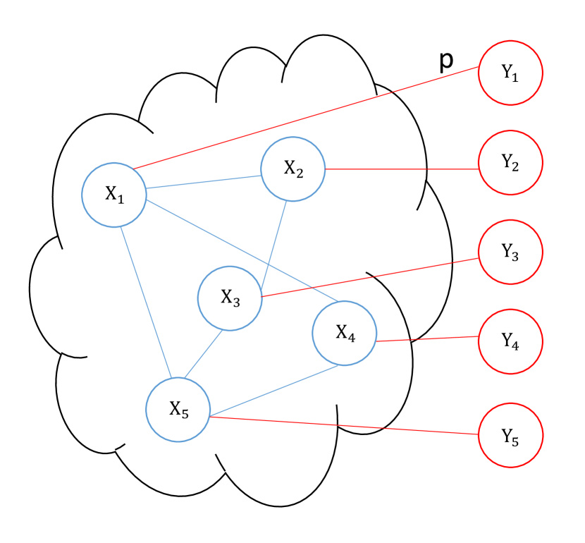
Figure 1: Markov Random Field model of sentiment detection.

The social network structure is modeled as an undirected graph, as shown in Fig. 1. Let 𝐗=(X1,,Xn)T{1,1}n𝐗superscriptsubscript𝑋1subscript𝑋𝑛𝑇superscript11𝑛\mathbf{X}=(X_{1},\dots,X_{n})^{T}\in\{-1,1\}^{n} denote the vector of binary sentiments of n𝑛n members, where 111 or 11-1 denote positive or negative sentiments respectively. These sentiments are unknown to observers. What is observed is a noisy measurement of 𝐗𝐗\mathbf{X}, called 𝐘𝐘\mathbf{Y}. 𝐘=(Y1,,Yn)T{1,1}n𝐘superscriptsubscript𝑌1subscript𝑌𝑛𝑇superscript11𝑛\mathbf{Y}=(Y_{1},\dots,Y_{n})^{T}\in\{-1,1\}^{n} is modeled as conditionally independent binary measurements of 𝐗𝐗\mathbf{X} each with cross-over probability p𝑝p, i.e., the output of a binary symmetric channel with input 𝐗𝐗\mathbf{X}. Without loss of generality, we assume that p<12𝑝12p<\frac{1}{2}. This model was first introduced in [7] for the ‘latent sentiment detection’ problem, with more details about the probability mass function of 𝐗𝐗\bf{X} following in Section II-B.

The majority sentiment is defined as

m=sign(𝟏T𝐗),𝑚signsuperscript1𝑇𝐗\displaystyle m=\text{sign}({\bf 1}^{T}{\bf X}), (1)

where 𝟏1{\bf 1} denotes the vector of all ones. We assume that n𝑛n is odd to avoid trivial ambiguity.

We will use the majority vote detector as our estimator for the majority sentiment:

m^=sign(𝟏T𝐘).^𝑚signsuperscript1𝑇𝐘\displaystyle\hat{m}=\text{sign}({\bf 1}^{T}{\bf Y}). (2)

This detector estimates the majority sentiment as the majority of noisy measurements. In general, it is not the optimal Maximum Aposteriori Probability (MAP) detector. However, it will be sufficient to illustrate the key insights of this paper, promised in Section I, as will be shown below.

The detection error probability (equivalently, classification error probability of the two sentiment class problem) is

Pe(n)=(mm^).subscriptsuperscript𝑃𝑛𝑒𝑚^𝑚\displaystyle P^{(n)}_{e}=\mathbb{P}(m\neq\hat{m}). (3)

We wish to investigate whether the majority sentiment detector is asymptotically accurate, i.e., whether Pe(n)subscriptsuperscript𝑃𝑛𝑒P^{(n)}_{e} becomes arbitrarily small when n𝑛n is sufficiently large.

In the paper, we denote Xn¯=1ni=1nXi¯subscript𝑋𝑛1𝑛superscriptsubscript𝑖1𝑛subscript𝑋𝑖\overline{X_{n}}=\frac{1}{n}\sum_{i=1}^{n}X_{i} as the sample average, Xlimsubscript𝑋X_{\lim} as a variable distributed as the limiting distribution of nXn¯𝑛¯subscript𝑋𝑛\sqrt{n}\,\overline{X_{n}}, and 𝑑𝑑\xrightarrow{d} as convergence in distribution.

II-A I.I.D Case

Before discussing interesting networks, let us first consider the simplest case: Xisubscript𝑋𝑖X_{i}s are independent and identical distributed (i.i.d.) random variables, taking values 11-1 or 111, each with probability 1/2121/2. In this example, the members are not connected, or in other words the network is an empty graph. This is the case in contemporary vote detection schemes where voters are assumed to independently vote, and the underlying network is not modeled [5]. For this case, the detector we adopt in (2) is actually the optimal MAP detector, so that there is no loss of error performance.

For this case, we can derive the exact value of the asymptotic error probability, as shown in Proposition 1.

Proposition 1

In the i.i.d. (empty graph) case,

limnPe=2πarcsinp>0.subscript𝑛subscript𝑃𝑒2𝜋𝑝0\lim_{n\to\infty}P_{e}=\frac{2}{\pi}\arcsin\sqrt{p}>0.
Proof.

Since (Xi,Yi)subscript𝑋𝑖subscript𝑌𝑖(X_{i},Y_{i})s are i.i.d. random variables, with means zero, and variances 𝔼[Xi2]=𝔼[Yi2]=1𝔼delimited-[]superscriptsubscript𝑋𝑖2𝔼delimited-[]superscriptsubscript𝑌𝑖21\mathbb{E}[X_{i}^{2}]=\mathbb{E}[Y_{i}^{2}]=1, 𝔼[XiYi]=12p𝔼delimited-[]subscript𝑋𝑖subscript𝑌𝑖12𝑝\mathbb{E}[X_{i}Y_{i}]=1-2p, the multidimensional central limit theorem tells that:

(nXn¯nYn¯)𝑑(XlimYlim)N((00),(112p12p1)).𝑑matrix𝑛¯subscript𝑋𝑛𝑛¯subscript𝑌𝑛matrixsubscript𝑋subscript𝑌similar-to𝑁matrix00matrix112𝑝12𝑝1\displaystyle\left(\begin{matrix}\sqrt{n}\,\overline{X_{n}}\\ \sqrt{n}\,\overline{Y_{n}}\end{matrix}\right)\xrightarrow{d}\left(\begin{matrix}X_{\lim}\\ Y_{\lim}\end{matrix}\right)\sim N\left(\left(\begin{matrix}0\\ 0\end{matrix}\right),\left(\begin{matrix}1&1-2p\\ 1-2p&1\end{matrix}\right)\right). (4)

Since by definition (3), Pe(n)=(nXn¯nYn¯<0)superscriptsubscript𝑃𝑒𝑛𝑛¯subscript𝑋𝑛𝑛¯subscript𝑌𝑛0P_{e}^{(n)}=\mathbb{P}(\sqrt{n}\,\overline{X_{n}}\sqrt{n}\,\overline{Y_{n}}<0), we can calculate its limit from (4) as

limnPe(n)subscript𝑛subscriptsuperscript𝑃𝑛𝑒\displaystyle\lim_{n\to\infty}P^{(n)}_{e} =(XlimYlim<0)=2πarcsinp,absentsubscript𝑋subscript𝑌02𝜋𝑝\displaystyle=\mathbb{P}(X_{\lim}Y_{\lim}<0)=\frac{2}{\pi}\arcsin\sqrt{p},

where the limit exists thanks to the convergence in distribution (4). ∎

In this special case, the detection error probability tends to some positive constant, and thus never reduces to 00, even with infinite number of sentiments. Inherently, this inaccuracy results from the absence of connections. This result is perhaps counterintuitive, since one may have expected that the majority sentiment can be detected accurately when the user size tends to infinity, as typically happens in the case of single parameter estimation.

II-B Network Model

The network model characterizes the probability mass function of 𝐗𝐗{\bf X}. In general, it could be any prior implying that members with connections are more probable to have the same sentiment. In this paper following [7], we adopt a homogeneous Ising MRF prior as

p(𝐱)=exp(θ𝐱TA𝐱)Zn(θ).𝑝𝐱𝜃superscript𝐱𝑇𝐴𝐱subscript𝑍𝑛𝜃\displaystyle p({\bf x})=\frac{\exp(\theta{\bf x}^{T}A{\bf x})}{Z_{n}(\theta)}. (5)

Here A𝐴A denotes the symmetric graph adjacency matrix, with Aij=0/1subscript𝐴𝑖𝑗01A_{ij}=0/1 denoting absence/presence of an edge respectively. θ>0𝜃0\theta>0 is called the inverse temperature parameter. We remark that θ𝜃\theta characterizes the connection strength in the network, namely, connected members are more probable to share the same sentiment in case of larger θ𝜃\theta. The normalizer Zn(θ)=𝐱{1,1}nexp(θ𝐱TA𝐱)subscript𝑍𝑛𝜃subscript𝐱superscript11𝑛𝜃superscript𝐱𝑇𝐴𝐱Z_{n}(\theta)=\sum_{\mathbf{x}\in\{-1,1\}^{n}}\exp(\theta{\bf x}^{T}A{\bf x}) is called the partition function.

The joint distribution of (𝐱,𝐲)𝐱𝐲({\bf x},{\bf y}) can be written as another Ising MRF as

p(𝐱,𝐲)=exp(θ𝐱TA𝐲+ε𝐲T𝐱)Zn(θ)(2coshε)n.𝑝𝐱𝐲𝜃superscript𝐱𝑇𝐴𝐲𝜀superscript𝐲𝑇𝐱subscript𝑍𝑛𝜃superscript2𝜀𝑛\displaystyle p(\mathbf{x},\mathbf{y})=\frac{\exp(\theta{\bf x}^{T}A{\bf y}+\varepsilon{\bf y}^{T}{\bf x})}{Z_{n}(\theta)(2\cosh\varepsilon)^{n}}. (6)

Here ε𝜀\varepsilon is defined by p=exp(ε)exp(ε)+exp(ε)𝑝𝜀𝜀𝜀p=\frac{\exp(-\varepsilon)}{\exp(\varepsilon)+\exp(-\varepsilon)}. In the next section, we analyze the asymptotic error probability under the above network model. For this purpose, we assume that as n𝑛n grows, there is a given sequence of graphs of n𝑛n vertices that models the OSN as (5).

III Error Probability under Network Model

In this section, we will first derive an upper bound for the detection error probability in Theorem 1, and two exact asymptotic results in Theorems 2 and 3, assuming a given sequence of graph adjacency matrices A𝐴A. After that, we will show that the asymptotic performance of the detection error probability is related to the concentration behavior of nXn¯𝑛¯subscript𝑋𝑛\sqrt{n}\,\overline{X_{n}} in Theorem 4.

Theorem 1
Pe(n)𝔼[exp((12p)28(1p)2(nXn¯)2)].superscriptsubscript𝑃𝑒𝑛𝔼delimited-[]superscript12𝑝28superscript1𝑝2superscript𝑛¯subscript𝑋𝑛2P_{e}^{(n)}\leq\mathbb{E}\left[\exp\left(\frac{-(1-2p)^{2}}{8(1-p)^{2}}(\sqrt{n}\,\overline{X_{n}})^{2}\right)\right].

Here the expectation is taken over 𝐗𝐗{\bf X}.

Proof.

Let Zi=Yi(12p)Xisubscript𝑍𝑖subscript𝑌𝑖12𝑝subscript𝑋𝑖Z_{i}=Y_{i}-(1-2p)X_{i}. Since Zisubscript𝑍𝑖Z_{i}s are conditionally independent given 𝐗𝐗{\bf X}, with 𝔼[Zi|𝐗]=0𝔼delimited-[]conditionalsubscript𝑍𝑖𝐗0\mathbb{E}[Z_{i}|{\bf X}]=0 and |Zi|2(1p)subscript𝑍𝑖21𝑝\lvert Z_{i}\rvert\leq 2(1-p), Hoeffding’s inequality tells that average Zn¯¯subscript𝑍𝑛\overline{Z_{n}} satisfies (nZn¯>ϵ𝐗)exp(ϵ28(1p)2)𝑛¯subscript𝑍𝑛conditionalitalic-ϵ𝐗superscriptitalic-ϵ28superscript1𝑝2\mathbb{P}(\sqrt{n}\,\overline{Z_{n}}>\epsilon\mid{\bf X})\leq\exp\left(\frac{-\epsilon^{2}}{8(1-p)^{2}}\right) and (nZn¯<ϵ𝐗)exp(ϵ28(1p)2)𝑛¯subscript𝑍𝑛braitalic-ϵ𝐗superscriptitalic-ϵ28superscript1𝑝2\mathbb{P}(\sqrt{n}\,\overline{Z_{n}}<-\epsilon\mid{\bf X})\leq\exp\left(\frac{-\epsilon^{2}}{8(1-p)^{2}}\right) for any ϵ>0italic-ϵ0\epsilon>0. By definition (3):

Pe(n)superscriptsubscript𝑃𝑒𝑛\displaystyle P_{e}^{(n)} =(nXn¯nYn¯<0)absent𝑛¯subscript𝑋𝑛𝑛¯subscript𝑌𝑛0\displaystyle=\mathbb{P}(\sqrt{n}\,\overline{X_{n}}\sqrt{n}\,\overline{Y_{n}}<0)
=(nXn¯nZn¯<(12p)(nXn¯)2)absent𝑛¯subscript𝑋𝑛𝑛¯subscript𝑍𝑛12𝑝superscript𝑛¯subscript𝑋𝑛2\displaystyle=\mathbb{P}(\sqrt{n}\,\overline{X_{n}}\sqrt{n}\,\overline{Z_{n}}<-(1-2p)(\sqrt{n}\,\overline{X_{n}})^{2})
=𝔼[(nXn¯nZn¯<(12p)(nXn¯)2𝐗)]absent𝔼delimited-[]𝑛¯subscript𝑋𝑛𝑛¯subscript𝑍𝑛bra12𝑝superscript𝑛¯subscript𝑋𝑛2𝐗\displaystyle=\mathbb{E}\left[\mathbb{P}(\sqrt{n}\,\overline{X_{n}}\sqrt{n}\,\overline{Z_{n}}<-(1-2p)(\sqrt{n}\,\overline{X_{n}})^{2}\mid{\bf X})\right] (7)
𝔼[exp((12p)28(1p)2(nXn¯)2)].absent𝔼delimited-[]superscript12𝑝28superscript1𝑝2superscript𝑛¯subscript𝑋𝑛2\displaystyle\leq\mathbb{E}\left[\exp\left(\frac{-(1-2p)^{2}}{8(1-p)^{2}}(\sqrt{n}\,\overline{X_{n}})^{2}\right)\right].

Theorem 2
lim infnPe(n)=lim infn𝔼[Q((12p)4p(1p)|nXn¯|)],subscriptlimit-infimum𝑛superscriptsubscript𝑃𝑒𝑛subscriptlimit-infimum𝑛𝔼delimited-[]𝑄12𝑝4𝑝1𝑝𝑛¯subscript𝑋𝑛\liminf_{n\to\infty}P_{e}^{(n)}=\liminf_{n\to\infty}\mathbb{E}\left[Q\left(\frac{(1-2p)}{\sqrt{4p(1-p)}}\left\lvert\sqrt{n}\,\overline{X_{n}}\right\rvert\right)\right],

where Q()𝑄Q(\cdot) is the tail probability of standard normal distribution: Q(x)=12πxexp(t2/2)𝑑t𝑄𝑥12𝜋superscriptsubscript𝑥superscript𝑡22differential-d𝑡Q(x)=\frac{1}{\sqrt{2\pi}}\int_{x}^{\infty}\exp(-t^{2}/2)dt.

Theorem 3
  1. (a)

    If nXn¯𝑑Φ𝑑𝑛¯subscript𝑋𝑛Φ\sqrt{n}\,\overline{X_{n}}\xrightarrow{d}\Phi, where ΦΦ\Phi is a distribution, then

    limnPe(n)=Q((12p)4p(1p)|x|)Φ(dx).subscript𝑛superscriptsubscript𝑃𝑒𝑛superscriptsubscript𝑄12𝑝4𝑝1𝑝𝑥Φ𝑑𝑥\lim_{n\to\infty}P_{e}^{(n)}=\int_{-\infty}^{\infty}Q\left(\frac{(1-2p)}{\sqrt{4p(1-p)}}\left\lvert x\right\rvert\right)\Phi(dx).
  2. (b)

    Specifically, if nXn¯𝑑N(0,σ2)𝑑𝑛¯subscript𝑋𝑛𝑁0superscript𝜎2\sqrt{n}\,\overline{X_{n}}\xrightarrow{d}N(0,\sigma^{2}), then

    limnPe(n)=1πarccot((12p)4p(1p)σ)>0.subscript𝑛superscriptsubscript𝑃𝑒𝑛1𝜋arccot12𝑝4𝑝1𝑝𝜎0\lim_{n\to\infty}P_{e}^{(n)}=\frac{1}{\pi}\operatorname{arccot}\left(\frac{(1-2p)}{\sqrt{4p(1-p)}}\sigma\right)>0.

To prove Theorems 2 and 3, we first derive a central limit theorem type result in Lemma 1. This will follow from the conditional independence of Yisubscript𝑌𝑖Y_{i}s given 𝐗𝐗{\bf X}, and reveals that n(Yn¯(12p)Xn¯)𝑛¯subscript𝑌𝑛12𝑝¯subscript𝑋𝑛\sqrt{n}\,(\overline{Y_{n}}-(1-2p)\overline{X_{n}}) tends to a normal distribution conditioned on 𝐗𝐗{\bf X}; besides that, when nXn¯𝑛¯subscript𝑋𝑛\sqrt{n}\overline{X_{n}} converges in distribution, the joint limiting distribution of n(Xn¯,Yn¯)𝑛¯subscript𝑋𝑛¯subscript𝑌𝑛\sqrt{n}(\overline{X_{n}},\overline{Y_{n}}) can also be obtained.

Lemma 1
  1. (a)

    Conditional convergence: For all 𝐗𝐗{\bf X},

    n(Yn¯(12p)Xn¯)𝐗𝑑N(0,4p(1p)).𝑑conditional𝑛¯subscript𝑌𝑛12𝑝¯subscript𝑋𝑛𝐗𝑁04𝑝1𝑝\sqrt{n}(\overline{Y_{n}}-(1-2p)\overline{X_{n}})\mid{\bf X}\xrightarrow{d}N(0,4p(1-p)).
  2. (b)

    Unconditional convergence:

    n(Yn¯(12p)Xn¯)𝑑N(0,4p(1p)).𝑑𝑛¯subscript𝑌𝑛12𝑝¯subscript𝑋𝑛𝑁04𝑝1𝑝\sqrt{n}(\overline{Y_{n}}-(1-2p)\overline{X_{n}})\xrightarrow{d}N(0,4p(1-p)).
  3. (c)

    Joint convergence: If nXn¯𝑑Φ𝑑𝑛¯subscript𝑋𝑛Φ\sqrt{n}\,\overline{X_{n}}\xrightarrow{d}\Phi, then

    n(Xn¯,Yn¯(12p)Xn¯)𝑑(Φ,N(0,4p(1p))),𝑑𝑛¯subscript𝑋𝑛¯subscript𝑌𝑛12𝑝¯subscript𝑋𝑛Φ𝑁04𝑝1𝑝\sqrt{n}\left(\overline{X_{n}},\overline{Y_{n}}-(1-2p)\overline{X_{n}}\right)\xrightarrow{d}\left(\Phi,N(0,4p(1-p))\right),

    where the two limiting distributions are independent.

Proof.

Let Zi=Yi(12p)Xisubscript𝑍𝑖subscript𝑌𝑖12𝑝subscript𝑋𝑖Z_{i}=Y_{i}-(1-2p)X_{i}. By Lévy’s continuity theorem [9], it is equivalent to prove the pointwise convergence of characteristic functions:

limnsubscript𝑛\displaystyle\lim_{n\to\infty} 𝔼[exp(jβnZn¯)|𝐗]=exp(4p(1p)β2/2),𝔼delimited-[]conditional𝑗𝛽𝑛¯subscript𝑍𝑛𝐗4𝑝1𝑝superscript𝛽22\displaystyle\mathbb{E}[\exp(j\beta\sqrt{n}\,\overline{Z_{n}})|{\bf X}]=\exp(-4p(1-p)\beta^{2}/2),
limnsubscript𝑛\displaystyle\lim_{n\to\infty} 𝔼[exp(jβnZn¯)]=exp(4p(1p)β2/2),𝔼delimited-[]𝑗𝛽𝑛¯subscript𝑍𝑛4𝑝1𝑝superscript𝛽22\displaystyle\mathbb{E}\left[\exp(j\beta\sqrt{n}\,\overline{Z_{n}})\right]=\exp(-4p(1-p)\beta^{2}/2),
limnsubscript𝑛\displaystyle\lim_{n\to\infty} 𝔼[exp(jωnXn¯+jβnZn¯)]=𝔼delimited-[]𝑗𝜔𝑛¯subscript𝑋𝑛𝑗𝛽𝑛¯subscript𝑍𝑛absent\displaystyle\mathbb{E}\left[\exp(j\omega\sqrt{n}\,\overline{X_{n}}+j\beta\sqrt{n}\,\overline{Z_{n}})\right]=
ϕ(ω)exp(4p(1p)β2/2),italic-ϕ𝜔4𝑝1𝑝superscript𝛽22\displaystyle\qquad\qquad\phi(\omega)\exp(-4p(1-p)\beta^{2}/2),

where ϕ()italic-ϕ\phi(\cdot) denotes the characteristic function of ΦΦ\Phi.

For part (a), since Zisubscript𝑍𝑖Z_{i}s are conditionally independent given 𝐗𝐗{\bf X}, with 𝔼[Zi|𝐗]=0𝔼delimited-[]conditionalsubscript𝑍𝑖𝐗0\mathbb{E}[Z_{i}|{\bf X}]=0, 𝔼[Zi2|𝐗]=4p(1p)𝔼delimited-[]conditionalsuperscriptsubscript𝑍𝑖2𝐗4𝑝1𝑝\mathbb{E}[Z_{i}^{2}|{\bf X}]=4p(1-p), and |Zi|2(1p)subscript𝑍𝑖21𝑝|Z_{i}|\leq 2(1-p), the Lindeberg condition: ϵ>0for-allitalic-ϵ0\forall\epsilon>0,

limn1n4p(1p)i=1n𝔼[Zi2I(|Zi|ϵn4p(1p))𝐗]=0subscript𝑛1𝑛4𝑝1𝑝superscriptsubscript𝑖1𝑛𝔼delimited-[]conditionalsubscriptsuperscript𝑍2𝑖𝐼subscript𝑍𝑖italic-ϵ𝑛4𝑝1𝑝𝐗0\lim_{n\to\infty}\frac{1}{n4p(1-p)}\sum_{i=1}^{n}\mathbb{E}\left[Z^{2}_{i}I\left(|Z_{i}|\geq\epsilon\sqrt{n4p(1-p)}\right)\mid{\bf X}\right]=0

is satisfied, where I()𝐼I(\cdot) is the indicator function. Lindeberg-Feller central limit theorem [9] tells that:

limn𝔼[exp(jβnZn¯)𝐗]=exp(4p(1p)β2/2),subscript𝑛𝔼delimited-[]conditional𝑗𝛽𝑛¯subscript𝑍𝑛𝐗4𝑝1𝑝superscript𝛽22\displaystyle\lim_{n\to\infty}\mathbb{E}[\exp(j\beta\sqrt{n}\,\overline{Z_{n}})\mid{\bf X}]=\exp(-4p(1-p)\beta^{2}/2), (8)

where RHS of (8) is the characteristic function of N(0,4p(1p))𝑁04𝑝1𝑝N(0,4p(1-p)).

For part (b), extend the result in (a) to the unconditional version. Notice that |𝔼[exp(jβnZn¯)𝐗]|1𝔼delimited-[]conditional𝑗𝛽𝑛¯subscript𝑍𝑛𝐗1\lvert\mathbb{E}[\exp(j\beta\sqrt{n}\,\overline{Z_{n}})\mid\mathbf{X}]\rvert\leq 1, thus

limnsubscript𝑛\displaystyle\lim_{n\to\infty} 𝔼[exp(jβnZn¯]=limn𝔼[𝔼[exp(jβnZn¯)𝐗]]\displaystyle\mathbb{E}[\exp(j\beta\sqrt{n}\,\overline{Z_{n}}]=\lim_{n\to\infty}\mathbb{E}\left[\mathbb{E}[\exp(j\beta\sqrt{n}\,\overline{Z_{n}})\mid\mathbf{X}]\right]
=𝔼[limn𝔼[exp(jβnZn¯)𝐗]]absent𝔼delimited-[]subscript𝑛𝔼delimited-[]conditional𝑗𝛽𝑛¯subscript𝑍𝑛𝐗\displaystyle=\mathbb{E}\left[\lim_{n\to\infty}\mathbb{E}[\exp(j\beta\sqrt{n}\,\overline{Z_{n}})\mid\mathbf{X}]\right]
=exp(4p(1p)β2/2),absent4𝑝1𝑝superscript𝛽22\displaystyle=\exp(-4p(1-p)\beta^{2}/2),

where the expectation and limit are exchanged by Lebesgue’s dominated convergence theorem [9].

For part (c), define Δn(𝐗)=𝔼[exp(jβnZn¯)𝐗]exp(4p(1p)β2/2)subscriptΔ𝑛𝐗𝔼delimited-[]conditional𝑗𝛽𝑛¯subscript𝑍𝑛𝐗4𝑝1𝑝superscript𝛽22\Delta_{n}({\bf X})=\mathbb{E}[\exp(j\beta\sqrt{n}\,\overline{Z_{n}})\mid\mathbf{X}]-\exp(-4p(1-p)\beta^{2}/2). By equation (8), limnΔn(𝐗)=0,𝐗subscript𝑛subscriptΔ𝑛𝐗0for-all𝐗\lim_{n\to\infty}\Delta_{n}({\bf X})=0,\forall{\bf X}. So,

limnsubscript𝑛\displaystyle\lim_{n\to\infty} 𝔼[exp(jωnXn¯+jβnZn¯)]𝔼delimited-[]𝑗𝜔𝑛¯subscript𝑋𝑛𝑗𝛽𝑛¯subscript𝑍𝑛\displaystyle\mathbb{E}\left[\exp(j\omega\sqrt{n}\,\overline{X_{n}}+j\beta\sqrt{n}\,\overline{Z_{n}})\right]
=limn𝔼[exp(jωnXn¯)𝔼[exp(jβnZn¯)𝐗]]absentsubscript𝑛𝔼delimited-[]𝑗𝜔𝑛¯subscript𝑋𝑛𝔼delimited-[]conditional𝑗𝛽𝑛¯subscript𝑍𝑛𝐗\displaystyle=\lim_{n\to\infty}\mathbb{E}\left[\exp(j\omega\sqrt{n}\,\overline{X_{n}})\mathbb{E}[\exp(j\beta\sqrt{n}\,\overline{Z_{n}})\mid\mathbf{X}]\right]
=limn𝔼[exp(jωnXn¯)exp(4p(1p)β2/2)]absentsubscript𝑛𝔼delimited-[]𝑗𝜔𝑛¯subscript𝑋𝑛4𝑝1𝑝superscript𝛽22\displaystyle=\lim_{n\to\infty}\mathbb{E}\left[\exp(j\omega\sqrt{n}\,\overline{X_{n}})\exp(-4p(1-p)\beta^{2}/2)\right]
+limn𝔼[exp(jωnXn¯)Δn(𝐗)]subscript𝑛𝔼delimited-[]𝑗𝜔𝑛¯subscript𝑋𝑛subscriptΔ𝑛𝐗\displaystyle\qquad+\lim_{n\to\infty}\mathbb{E}[\exp(j\omega\sqrt{n}\,\overline{X_{n}})\Delta_{n}(\mathbf{X})] (9)
=ϕ(ω)exp(4p(1p)β2/2).absentitalic-ϕ𝜔4𝑝1𝑝superscript𝛽22\displaystyle=\phi(\omega)\exp(-4p(1-p)\beta^{2}/2).

In equation (9), since |Δn(𝐗)|2subscriptΔ𝑛𝐗2\lvert\Delta_{n}({\bf X})\rvert\leq 2 is bounded, limn𝔼[exp(jωnXn¯)Δn(𝐗)]=0subscript𝑛𝔼delimited-[]𝑗𝜔𝑛¯subscript𝑋𝑛subscriptΔ𝑛𝐗0\lim_{n\to\infty}\mathbb{E}[\exp(j\omega\sqrt{n}\,\overline{X_{n}})\Delta_{n}(\mathbf{X})]=0 by Lebesgue’s dominated convergence theorem [9]. ∎

Now we use Lemma 1 to prove Theorems 2 and 3.

Theorem 2.

Start from equation (III). Define εn(𝐗)=(nXn¯nZn¯<(12p)(nXn¯)2𝐗)Q((12p)4p(1p)|nXn¯|)subscript𝜀𝑛𝐗𝑛¯subscript𝑋𝑛𝑛¯subscript𝑍𝑛bra12𝑝superscript𝑛¯subscript𝑋𝑛2𝐗𝑄12𝑝4𝑝1𝑝𝑛¯subscript𝑋𝑛\varepsilon_{n}({\bf X})=\mathbb{P}(\sqrt{n}\,\overline{X_{n}}\sqrt{n}\,\overline{Z_{n}}<-(1-2p)(\sqrt{n}\,\overline{X_{n}})^{2}\mid{\bf X})-Q\left(\frac{(1-2p)}{\sqrt{4p(1-p)}}\left\lvert\sqrt{n}\,\overline{X_{n}}\right\rvert\right). From the limiting distribution in Lemma 1 part (a), limnεn(𝐗)=0,𝐗subscript𝑛subscript𝜀𝑛𝐗0for-all𝐗\lim_{n\to\infty}\varepsilon_{n}({\bf X})=0,\forall{\bf X}. So,

lim infnPe(n)subscriptlimit-infimum𝑛superscriptsubscript𝑃𝑒𝑛\displaystyle\liminf_{n\to\infty}P_{e}^{(n)} =lim infn𝔼[(nXn¯nZn¯<\displaystyle=\liminf_{n\to\infty}\mathbb{E}[\mathbb{P}(\sqrt{n}\,\overline{X_{n}}\sqrt{n}\,\overline{Z_{n}}<
(12p)(nXn¯)2𝐗)]\displaystyle\qquad\qquad\qquad-(1-2p)(\sqrt{n}\,\overline{X_{n}})^{2}\mid{\bf X})]
=lim infn𝔼[Q((12p)4p(1p)|nXn¯|)]absentsubscriptlimit-infimum𝑛𝔼delimited-[]𝑄12𝑝4𝑝1𝑝𝑛¯subscript𝑋𝑛\displaystyle=\liminf_{n\to\infty}\mathbb{E}\left[Q\left(\frac{(1-2p)}{\sqrt{4p(1-p)}}\left\lvert\sqrt{n}\,\overline{X_{n}}\right\rvert\right)\right]
+lim infn𝔼[εn(𝐗)]subscriptlimit-infimum𝑛𝔼delimited-[]subscript𝜀𝑛𝐗\displaystyle\qquad\qquad\qquad+\liminf_{n\to\infty}\mathbb{E}\left[\varepsilon_{n}({\bf X})\right]
=lim infn𝔼[Q((12p)4p(1p)|nXn¯|)].absentsubscriptlimit-infimum𝑛𝔼delimited-[]𝑄12𝑝4𝑝1𝑝𝑛¯subscript𝑋𝑛\displaystyle=\liminf_{n\to\infty}\mathbb{E}\left[Q\left(\frac{(1-2p)}{\sqrt{4p(1-p)}}\left\lvert\sqrt{n}\,\overline{X_{n}}\right\rvert\right)\right].

Here lim infn𝔼[εn(𝐗)]=𝔼[lim infnεn(𝐗)]=0subscriptlimit-infimum𝑛𝔼delimited-[]subscript𝜀𝑛𝐗𝔼delimited-[]subscriptlimit-infimum𝑛subscript𝜀𝑛𝐗0\liminf_{n\to\infty}\mathbb{E}\left[\varepsilon_{n}({\bf X})\right]=\mathbb{E}\left[\liminf_{n\to\infty}\varepsilon_{n}({\bf X})\right]=0 by Lebesgue’s dominated convergence theorem [9], since |εn(𝐗)|1subscript𝜀𝑛𝐗1\lvert\varepsilon_{n}({\bf X})\rvert\leq 1. ∎

Theorem 3.

Mimic the proof of Theorem 2, with all ‘lim inflimit-infimum\liminf’ replaced by ‘lim\lim’. ∎

Finally, based on Theorems 1, 2 and 3, we prove Theorem 4: whether the detection error probability tends to 00 is exactly determined by whether nXn¯𝑛¯subscript𝑋𝑛\sqrt{n}\,\overline{X_{n}} asymptotically stays away from 00, in probability.

Theorem 4
  1. (a)

    If B>0for-all𝐵0\forall B>0, limn(|nXn¯|B)=0subscript𝑛𝑛¯subscript𝑋𝑛𝐵0\lim_{n\to\infty}\mathbb{P}(\lvert\sqrt{n}\,\overline{X_{n}}\rvert\leq B)=0, then limnPe(n)=0subscript𝑛superscriptsubscript𝑃𝑒𝑛0\lim_{n\to\infty}P_{e}^{(n)}=0.

  2. (b)

    If B>0𝐵0\exists B>0 s.t. lim infn(|nXn¯|B)>0subscriptlimit-infimum𝑛𝑛¯subscript𝑋𝑛𝐵0\liminf_{n\to\infty}\mathbb{P}(\lvert\sqrt{n}\,\overline{X_{n}}\rvert\leq B)>0, then lim infnPe(n)>0subscriptlimit-infimum𝑛superscriptsubscript𝑃𝑒𝑛0\liminf_{n\to\infty}P_{e}^{(n)}>0.

As a comparison to statistical physics, part (a) corresponds to the ferromagnetic phase where spins are mostly in one direction; part (b) corresponds to the paramagnetic phase where spins are nearly equal in both directions.

Proof.

For part (a), given any ϵ>0italic-ϵ0\epsilon>0, choose B𝐵B large enough such that exp((12p)28(1p)2B2)ϵ/2superscript12𝑝28superscript1𝑝2superscript𝐵2italic-ϵ2\exp\left(\frac{-(1-2p)^{2}}{8(1-p)^{2}}B^{2}\right)\leq\epsilon/2, then choose n𝑛n large enough such that (|nXn¯|B)ϵ/2𝑛¯subscript𝑋𝑛𝐵italic-ϵ2\mathbb{P}(\lvert\sqrt{n}\,\overline{X_{n}}\rvert\leq B)\leq\epsilon/2. Theorem 1 tells that

Pe(n)superscriptsubscript𝑃𝑒𝑛\displaystyle P_{e}^{(n)} 𝔼[exp((12p)28(1p)2(nXn¯)2)]absent𝔼delimited-[]superscript12𝑝28superscript1𝑝2superscript𝑛¯subscript𝑋𝑛2\displaystyle\leq\mathbb{E}\left[\exp\left(\frac{-(1-2p)^{2}}{8(1-p)^{2}}(\sqrt{n}\,\overline{X_{n}})^{2}\right)\right]
(|nXn¯|B)+exp((12p)28(1p)2B2)ϵ.absent𝑛¯subscript𝑋𝑛𝐵superscript12𝑝28superscript1𝑝2superscript𝐵2italic-ϵ\displaystyle\leq\mathbb{P}(\lvert\sqrt{n}\,\overline{X_{n}}\rvert\leq B)+\exp\left(\frac{-(1-2p)^{2}}{8(1-p)^{2}}B^{2}\right)\leq\epsilon.

Thus limnPe(n)=0subscript𝑛superscriptsubscript𝑃𝑒𝑛0\lim_{n\to\infty}P_{e}^{(n)}=0.

For part (b), choose a B>0𝐵0B>0, such that lim infn(|nXn¯|B)>0subscriptlimit-infimum𝑛𝑛¯subscript𝑋𝑛𝐵0\liminf_{n\to\infty}\mathbb{P}(\lvert\sqrt{n}\,\overline{X_{n}}\rvert\leq B)>0. Theorem 2 tells that

lim infnsubscriptlimit-infimum𝑛\displaystyle\liminf_{n\to\infty} Pe(n)=lim infn𝔼[Q((12p)4p(1p)|nXn¯|)]superscriptsubscript𝑃𝑒𝑛subscriptlimit-infimum𝑛𝔼delimited-[]𝑄12𝑝4𝑝1𝑝𝑛¯subscript𝑋𝑛\displaystyle P_{e}^{(n)}=\liminf_{n\to\infty}\mathbb{E}\left[Q\left(\frac{(1-2p)}{\sqrt{4p(1-p)}}\left\lvert\sqrt{n}\,\overline{X_{n}}\right\rvert\right)\right]
lim infn(|nXn¯|B)Q((12p)4p(1p)B)>0.absentsubscriptlimit-infimum𝑛𝑛¯subscript𝑋𝑛𝐵𝑄12𝑝4𝑝1𝑝𝐵0\displaystyle\geq\liminf_{n\to\infty}\mathbb{P}(\lvert\sqrt{n}\,\overline{X_{n}}\rvert\leq B)Q\left(\frac{(1-2p)}{\sqrt{4p(1-p)}}B\right)>0.

IV Network Examples

Given a network topology (i.e., graph adjacency matrix A𝐴A), theorems in the previous section characterize the asymptotic performance of the detection error probability. In this section, we will discuss two extreme network examples of Fig. 1: the chain graph (1-D Markov chain), and the complete graph. We will show that in the chain graph (as well as the empty graph as shown in Section II-A), the detection error probability is asymptotically positive; in contrast, in the complete graph there exists a phenomenon of phase transition, where the detection error tends to 00 when the connection strength is more than some critical value, while it is asymptotically positive when the connection strength is less than that critical value. This is similar to the paramagnetic-ferromagnetic phase transition in statistical physics!

IV-A Chain Graph

In a chain graph, each vertex is connected to two neighbors, forming a chain. For convenience, we adopt a periodical boundary condition (PBC), namely, the n𝑛nth member is connected with the first member; nevertheless, boundary conditions asymptotically make no difference. It can be viewed as a Markov chain as: Xi+1={Xi,w.p.exp(θ)exp(θ)+exp(θ)Xi,w.p.exp(θ)exp(θ)+exp(θ),i=1,n,X_{i+1}=\left\{\begin{matrix}X_{i},&w.p.~{}\frac{\exp(\theta)}{\exp(\theta)+\exp(-\theta)}\\ -X_{i},&w.p.~{}\frac{\exp(-\theta)}{\exp(\theta)+\exp(-\theta)}\end{matrix}\right.,i=1,\dots n, with Xn+1subscript𝑋𝑛1X_{n+1} treated as X1subscript𝑋1X_{1}. We will prove that the detection error probability is asymptotically positive, in Proposition 2 below.

Proposition 2

In the chain graph,

limnPe(n)=1πarccot((12p)4p(1p)eθ)>0.subscript𝑛superscriptsubscript𝑃𝑒𝑛1𝜋arccot12𝑝4𝑝1𝑝superscript𝑒𝜃0\lim_{n\to\infty}P_{e}^{(n)}=\frac{1}{\pi}\operatorname{arccot}\left(\frac{(1-2p)}{\sqrt{4p(1-p)}}e^{\theta}\right)>0.
Proof.

In the chain graph, the partition function at field b𝑏b, defined by Zn(θ,b)=𝐱{1,1}nexp(θ(x1x2++xn1xn+xnx1)+b𝟏T𝐱)subscript𝑍𝑛𝜃𝑏subscript𝐱superscript11𝑛𝜃subscript𝑥1subscript𝑥2subscript𝑥𝑛1subscript𝑥𝑛subscript𝑥𝑛subscript𝑥1𝑏superscript1𝑇𝐱Z_{n}(\theta,b)=\sum_{{\bf x}\in\{-1,1\}^{n}}\exp(\theta(x_{1}x_{2}+\cdots+x_{n-1}x_{n}+x_{n}x_{1})+b{\bf 1}^{T}{\bf x}), is [10]

Zn(θ,b)subscript𝑍𝑛𝜃𝑏\displaystyle Z_{n}(\theta,b) =enθ(coshb+sinh2b+e4θ)nabsentsuperscript𝑒𝑛𝜃superscript𝑏superscript2𝑏superscript𝑒4𝜃𝑛\displaystyle=e^{n\theta}\left(\cosh b+\sqrt{\sinh^{2}b+e^{-4\theta}}\right)^{n}
+enθ(coshbsinh2b+e4θ)n.superscript𝑒𝑛𝜃superscript𝑏superscript2𝑏superscript𝑒4𝜃𝑛\displaystyle\qquad+e^{n\theta}\left(\cosh b-\sqrt{\sinh^{2}b+e^{-4\theta}}\right)^{n}. (10)

Plug b=0𝑏0b=0 into (IV-A) to get Zn(θ)Zn(θ,0)=(2coshθ)n+(2sinhθ)napproaches-limitsubscript𝑍𝑛𝜃subscript𝑍𝑛𝜃0superscript2𝜃𝑛superscript2𝜃𝑛Z_{n}(\theta)\doteq Z_{n}(\theta,0)=(2\cosh\theta)^{n}+(2\sinh\theta)^{n}.

The characteristic function of nXn¯𝑛¯subscript𝑋𝑛\sqrt{n}\,\overline{X_{n}} is

limnsubscript𝑛\displaystyle\lim_{n\to\infty} 𝔼[exp(jωnXn¯)]𝔼delimited-[]𝑗𝜔𝑛¯subscript𝑋𝑛\displaystyle\mathbb{E}\left[\exp(j\omega\sqrt{n}\,\overline{X_{n}})\right]
=limn1Zn(θ)𝐱{1,1}nexp(θ(x1x2++xnx1)\displaystyle=\lim_{n\to\infty}\frac{1}{Z_{n}(\theta)}\sum\limits_{{\bf x}\in\{-1,1\}^{n}}\exp(\theta(x_{1}x_{2}+\cdots+x_{n}x_{1})
+jωnXn¯)\displaystyle\qquad+j\omega\sqrt{n}\,\overline{X_{n}})
=limnZn(θ,jωn)Zn(θ)absentsubscript𝑛subscript𝑍𝑛𝜃𝑗𝜔𝑛subscript𝑍𝑛𝜃\displaystyle=\lim_{n\to\infty}\frac{Z_{n}(\theta,\frac{j\omega}{\sqrt{n}})}{Z_{n}(\theta)}
=limnenθ(coshjωn+sinh2jωn+e4θ)n(2coshθ)n+(2sinhθ)nabsentsubscript𝑛superscript𝑒𝑛𝜃superscript𝑗𝜔𝑛superscript2𝑗𝜔𝑛superscript𝑒4𝜃𝑛superscript2𝜃𝑛superscript2𝜃𝑛\displaystyle=\lim_{n\to\infty}\frac{e^{n\theta}\left(\cosh\frac{j\omega}{\sqrt{n}}+\sqrt{\sinh^{2}\frac{j\omega}{\sqrt{n}}+e^{-4\theta}}\right)^{n}}{(2\cosh\theta)^{n}+(2\sinh\theta)^{n}}
+limnenθ(coshjωnsinh2jωn+e4θ)n(2coshθ)n+(2sinhθ)nsubscript𝑛superscript𝑒𝑛𝜃superscript𝑗𝜔𝑛superscript2𝑗𝜔𝑛superscript𝑒4𝜃𝑛superscript2𝜃𝑛superscript2𝜃𝑛\displaystyle\qquad+\lim_{n\to\infty}\frac{e^{n\theta}\left(\cosh\frac{j\omega}{\sqrt{n}}-\sqrt{\sinh^{2}\frac{j\omega}{\sqrt{n}}+e^{-4\theta}}\right)^{n}}{(2\cosh\theta)^{n}+(2\sinh\theta)^{n}} (11)
=exp(e2θω2/2).absentsuperscript𝑒2𝜃superscript𝜔22\displaystyle=\exp\left(-e^{2\theta}\omega^{2}/2\right).

In equation (11), we use Taylor’s expansions of coshjωn𝑗𝜔𝑛\cosh\frac{j\omega}{\sqrt{n}} and sinhjωn𝑗𝜔𝑛\sinh\frac{j\omega}{\sqrt{n}} to calculate the limit. As a result, nXn¯𝑑N(0,e2θ)𝑑𝑛¯subscript𝑋𝑛𝑁0superscript𝑒2𝜃\sqrt{n}\,\overline{X_{n}}\xrightarrow{d}N\left(0,e^{2\theta}\right). So, Theorem 3 tells that:

limnPe(n)=1πarccot((12p)4p(1p)eθ)>0.subscript𝑛superscriptsubscript𝑃𝑒𝑛1𝜋arccot12𝑝4𝑝1𝑝superscript𝑒𝜃0\lim_{n\to\infty}P_{e}^{(n)}=\frac{1}{\pi}\operatorname{arccot}\left(\frac{(1-2p)}{\sqrt{4p(1-p)}}e^{\theta}\right)>0.

IV-B Complete Graph

In a complete graph, each pair of vertices is connected. The corresponding Ising MRF prior (12), also called the Curie-Weiss [11] prior, is defined slightly differently, in that the strength is weakened to θ/n𝜃𝑛\theta/n, to ensure that the total strength from all neighbors of a vertex remains constant, i.e., does not grow with n𝑛n, though the number of neighbors is n1𝑛1n-1. Thus, with this standard modification, the prior is

p(𝐱)=exp(θn(𝟏T𝐱)2)Zn(θ).𝑝𝐱𝜃𝑛superscriptsuperscript1𝑇𝐱2subscript𝑍𝑛𝜃\displaystyle p({\bf x})=\frac{\exp\left(\frac{\theta}{n}({\bf 1}^{T}{\bf x})^{2}\right)}{Z_{n}(\theta)}. (12)

We are interested in the limiting distribution of nXn¯𝑛¯subscript𝑋𝑛\sqrt{n}\,\overline{X_{n}}, with the corresponding variable called Xlimsubscript𝑋X_{\lim}. Intuitively, it should have the density p(xlim)exp(θxlim2)exp(xlim2/2)proportional-to𝑝subscript𝑥𝜃superscriptsubscript𝑥2superscriptsubscript𝑥22p(x_{\lim})\propto\exp(\theta x_{\lim}^{2})\exp(-x_{\lim}^{2}/2), since in the i.i.d. case nXn¯𝑑N(0,1)𝑑𝑛¯subscript𝑋𝑛𝑁01\sqrt{n}\,\overline{X_{n}}\xrightarrow{d}N(0,1), and the Curie-Weiss prior introduces a multiplier exp(θxlim2)𝜃superscriptsubscript𝑥2\exp(\theta x_{\lim}^{2}). In the case θ<12𝜃12\theta<\frac{1}{2}, nXn¯𝑛¯subscript𝑋𝑛\sqrt{n}\,\overline{X_{n}} converges to a normal distribution, and therefore, by Theorem 3, the detection error probability should be asymptotically positive; otherwise nXn¯𝑛¯subscript𝑋𝑛\sqrt{n}\,\overline{X_{n}} diverges so the error probability should tend to 00. We shall prove all these formally in Proposition 3.

Proposition 3

In the complete graph,

  1. (a)

    if θ<12𝜃12\theta<\frac{1}{2}, then

    limnPe(n)=1πarccot((12p)4p(1p)112θ)>0.subscript𝑛superscriptsubscript𝑃𝑒𝑛1𝜋arccot12𝑝4𝑝1𝑝112𝜃0\lim_{n\to\infty}P_{e}^{(n)}=\frac{1}{\pi}\operatorname{arccot}\left(\frac{(1-2p)}{\sqrt{4p(1-p)}}\frac{1}{\sqrt{1-2\theta}}\right)>0.
  2. (b)

    if θ>12𝜃12\theta>\frac{1}{2}, then limnPe(n)=0subscript𝑛superscriptsubscript𝑃𝑒𝑛0\lim_{n\to\infty}P_{e}^{(n)}=0. In fact, it tends to 00 exponentially fast: lim infn1nlogPe(n)>0subscriptlimit-infimum𝑛1𝑛superscriptsubscript𝑃𝑒𝑛0\liminf_{n\to\infty}-\frac{1}{n}\log P_{e}^{(n)}>0.

Proof.

In this model, the partition function at field b𝑏b, defined by Zn(θ,b)=𝐱{1,1}nexp(θn(𝟏T𝐱)2+b𝟏T𝐱)subscript𝑍𝑛𝜃𝑏subscript𝐱superscript11𝑛𝜃𝑛superscriptsuperscript1𝑇𝐱2𝑏superscript1𝑇𝐱Z_{n}(\theta,b)=\sum_{{\bf x}\in\{-1,1\}^{n}}\exp(\frac{\theta}{n}({\bf 1}^{T}{\bf x})^{2}+b{\bf 1}^{T}{\bf x}), is [11]

Zn(θ,b)=2nπexp(t2)coshn(2θnt+b)𝑑t.subscript𝑍𝑛𝜃𝑏superscript2𝑛𝜋superscriptsubscriptsuperscript𝑡2superscript𝑛2𝜃𝑛𝑡𝑏differential-d𝑡\displaystyle Z_{n}(\theta,b)=\frac{2^{n}}{\sqrt{\pi}}\int_{-\infty}^{\infty}\exp(-t^{2})\cosh^{n}\left(2\sqrt{\frac{\theta}{n}}t+b\right)dt. (13)

For part (a), we calculate the characteristic function of nXn¯𝑛¯subscript𝑋𝑛\sqrt{n}\,\overline{X_{n}} as

limnsubscript𝑛\displaystyle\lim_{n\to\infty} 𝔼[exp(jωnXn¯)]=limnZn(θ,jωn)Zn(θ)𝔼delimited-[]𝑗𝜔𝑛¯subscript𝑋𝑛subscript𝑛subscript𝑍𝑛𝜃𝑗𝜔𝑛subscript𝑍𝑛𝜃\displaystyle\mathbb{E}\left[\exp(j\omega\sqrt{n}\,\overline{X_{n}})\right]=\lim_{n\to\infty}\frac{Z_{n}(\theta,\frac{j\omega}{\sqrt{n}})}{Z_{n}(\theta)}
=exp(t2)limncoshn(2θnt+jωn)dtexp(t2)limncoshn(2θnt)dtabsentsuperscriptsubscriptsuperscript𝑡2subscript𝑛superscript𝑛2𝜃𝑛𝑡𝑗𝜔𝑛𝑑𝑡superscriptsubscriptsuperscript𝑡2subscript𝑛superscript𝑛2𝜃𝑛𝑡𝑑𝑡\displaystyle=\frac{\int_{-\infty}^{\infty}\exp(-t^{2})\lim_{n\to\infty}\cosh^{n}\left(2\sqrt{\frac{\theta}{n}}t+\frac{j\omega}{\sqrt{n}}\right)dt}{\int_{-\infty}^{\infty}\exp(-t^{2})\lim_{n\to\infty}\cosh^{n}\left(2\sqrt{\frac{\theta}{n}}t\right)dt}
=exp(t2)exp(12(2θt+jω)2)𝑑texp(t2)exp(12(2θt)2)𝑑tabsentsuperscriptsubscriptsuperscript𝑡212superscript2𝜃𝑡𝑗𝜔2differential-d𝑡superscriptsubscriptsuperscript𝑡212superscript2𝜃𝑡2differential-d𝑡\displaystyle=\frac{\int_{-\infty}^{\infty}\exp(-t^{2})\exp\left(\frac{1}{2}(2\sqrt{\theta}t+j\omega)^{2}\right)dt}{\int_{-\infty}^{\infty}\exp(-t^{2})\exp\left(\frac{1}{2}(2\sqrt{\theta}t)^{2}\right)dt}
=exp(ω22(12θ)).absentsuperscript𝜔2212𝜃\displaystyle=\exp\left(-\frac{\omega^{2}}{2(1-2\theta)}\right).

In the second line, the integral and the limit are exchanged by monotone convergence theorem [9]. In the third line, we use the Gaussian integral formula: exp(x2)𝑑x=πsuperscriptsubscriptsuperscript𝑥2differential-d𝑥𝜋\int_{-\infty}^{\infty}\exp(-x^{2})dx=\sqrt{\pi}, with appropriate changes of variables. As a result, nXn¯𝑑N(0,112θ)𝑑𝑛¯subscript𝑋𝑛𝑁0112𝜃\sqrt{n}\,\overline{X_{n}}\xrightarrow{d}N\left(0,\frac{1}{1-2\theta}\right). So, Theorem 3 tells that

limnPe(n)=1πarccot((12p)4p(1p)112θ)>0.subscript𝑛superscriptsubscript𝑃𝑒𝑛1𝜋arccot12𝑝4𝑝1𝑝112𝜃0\lim_{n\to\infty}P_{e}^{(n)}=\frac{1}{\pi}\operatorname{arccot}\left(\frac{(1-2p)}{\sqrt{4p(1-p)}}\frac{1}{\sqrt{1-2\theta}}\right)>0.

For part (b), we only need to prove that lim infn1nlogPe(n)>0subscriptlimit-infimum𝑛1𝑛superscriptsubscript𝑃𝑒𝑛0\liminf_{n\to\infty}-\frac{1}{n}\log P_{e}^{(n)}>0. Define Cp=(12p)28(1p)2subscript𝐶𝑝superscript12𝑝28superscript1𝑝2C_{p}=\frac{(1-2p)^{2}}{8(1-p)^{2}}. Start from Theorem 1:

Pe(n)superscriptsubscript𝑃𝑒𝑛\displaystyle P_{e}^{(n)} 𝔼[exp(Cp(nXn¯)2)]absent𝔼delimited-[]subscript𝐶𝑝superscript𝑛¯subscript𝑋𝑛2\displaystyle\leq\mathbb{E}\left[\exp\left(-C_{p}(\sqrt{n}\,\overline{X_{n}})^{2}\right)\right]
=1Zn(θ)𝐱{1,1}nexp(θn(𝟏T𝐱)2Cp(nXn¯)2)absent1subscript𝑍𝑛𝜃subscript𝐱superscript11𝑛𝜃𝑛superscriptsuperscript1𝑇𝐱2subscript𝐶𝑝superscript𝑛¯subscript𝑋𝑛2\displaystyle=\frac{1}{Z_{n}(\theta)}\sum_{{\bf x}\in\{-1,1\}^{n}}\exp\left(\frac{\theta}{n}({\bf 1}^{T}{\bf x})^{2}-C_{p}(\sqrt{n}\,\overline{X_{n}})^{2}\right)
=Zn(θCp)Zn(θ)absentsubscript𝑍𝑛𝜃subscript𝐶𝑝subscript𝑍𝑛𝜃\displaystyle=\frac{Z_{n}(\theta-C_{p})}{Z_{n}(\theta)}
=exp(t2)coshn(2θCpnt)𝑑texp(t2)coshn(2θnt)𝑑tabsentsuperscriptsubscriptsuperscript𝑡2superscript𝑛2𝜃subscript𝐶𝑝𝑛𝑡differential-d𝑡superscriptsubscriptsuperscript𝑡2superscript𝑛2𝜃𝑛𝑡differential-d𝑡\displaystyle=\frac{\int_{-\infty}^{\infty}\exp(-t^{2})\cosh^{n}\left(2\sqrt{\frac{\theta-C_{p}}{n}}t\right)dt}{\int_{-\infty}^{\infty}\exp(-t^{2})\cosh^{n}\left(2\sqrt{\frac{\theta}{n}}t\right)dt}
=exp(ns2+nlogcosh(2θCps))𝑑sexp(ns2+nlogcosh(2θs))𝑑s.absentsuperscriptsubscript𝑛superscript𝑠2𝑛2𝜃subscript𝐶𝑝𝑠differential-d𝑠superscriptsubscript𝑛superscript𝑠2𝑛2𝜃𝑠differential-d𝑠\displaystyle=\frac{\int_{-\infty}^{\infty}\exp(-ns^{2}+n\log\cosh(2\sqrt{\theta-C_{p}}s))ds}{\int_{-\infty}^{\infty}\exp(-ns^{2}+n\log\cosh(2\sqrt{\theta}s))ds}. (14)

In the fourth line, we use formula (13), with Z(θ)Z(θ,0)approaches-limit𝑍𝜃𝑍𝜃0Z(\theta)\doteq Z(\theta,0). In the fifth line, we change the variable to s=t/n𝑠𝑡𝑛s=t/\sqrt{n}.

Define f(θ,s)=logcosh(2θs)s2𝑓𝜃𝑠2𝜃𝑠superscript𝑠2f(\theta,s)=\log\cosh(2\sqrt{\theta}s)-s^{2}. From equation (14) we obtain that:

1nlogPe(n)1𝑛superscriptsubscript𝑃𝑒𝑛\displaystyle-\frac{1}{n}\log P_{e}^{(n)} 1nlogexp(nf(θ,s))𝑑sabsent1𝑛superscriptsubscript𝑛𝑓𝜃𝑠differential-d𝑠\displaystyle\geq\frac{1}{n}\log\int_{-\infty}^{\infty}\exp(nf(\theta,s))ds
1nlogexp(nf(θCp,s))𝑑s.1𝑛superscriptsubscript𝑛𝑓𝜃subscript𝐶𝑝𝑠differential-d𝑠\displaystyle\qquad-\frac{1}{n}\log\int_{-\infty}^{\infty}\exp(nf(\theta-C_{p},s))ds.

By Laplace’s approximation [12], listed below as Lemma 2, whose conditions are satisfied by f(θ,s)𝑓𝜃𝑠f(\theta,s) when θ>12𝜃12\theta>\frac{1}{2}, limn1nlogexp(nf(θ,s))𝑑s=maxsf(θ,s)subscript𝑛1𝑛superscriptsubscript𝑛𝑓𝜃𝑠differential-d𝑠subscript𝑠𝑓𝜃𝑠\lim_{n\to\infty}\frac{1}{n}\log\int_{-\infty}^{\infty}\exp(nf(\theta,s))ds=\max_{s}f(\theta,s), and similarly for the second term.

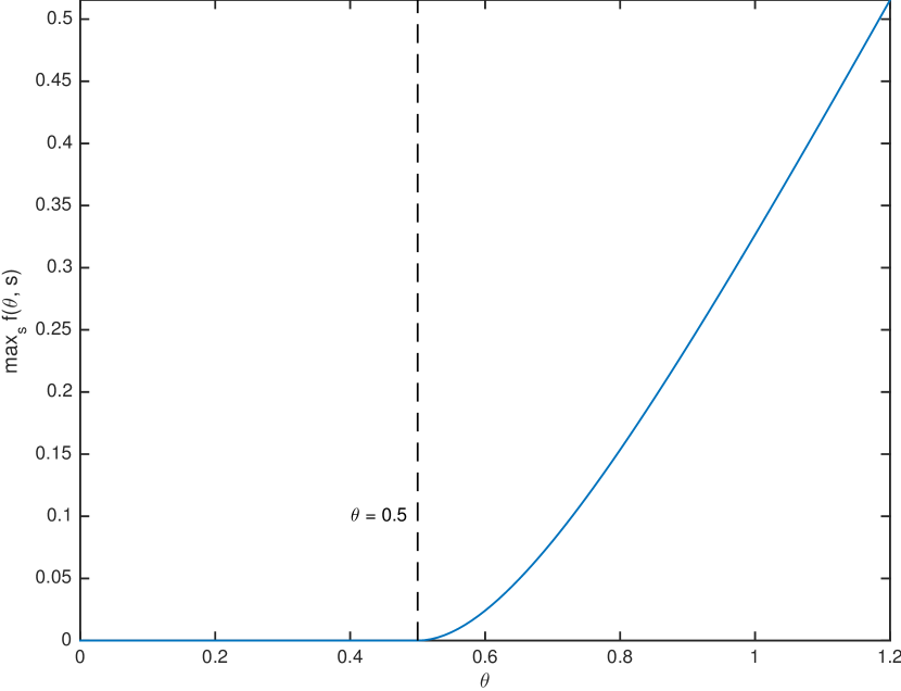
It can be observed (proof is omitted here) that maxsf(θ,s)subscript𝑠𝑓𝜃𝑠\max_{s}f(\theta,s) is 00 when θ12𝜃12\theta\leq\frac{1}{2} and monotonically increases with θ𝜃\theta when θ>12𝜃12\theta>\frac{1}{2}, as illustrated in Fig. 2. Under the condition θ>12𝜃12\theta>\frac{1}{2}, noticing that 0<Cp180subscript𝐶𝑝180<C_{p}\leq\frac{1}{8} by definition, we state that maxsf(θ,s)>maxsf(θCp,s)subscript𝑠𝑓𝜃𝑠subscript𝑠𝑓𝜃subscript𝐶𝑝𝑠\max_{s}f(\theta,s)>\max_{s}f(\theta-C_{p},s). In conclusion,

lim infn1nlogPe(n)subscriptlimit-infimum𝑛1𝑛superscriptsubscript𝑃𝑒𝑛\displaystyle\liminf_{n\to\infty}-\frac{1}{n}\log P_{e}^{(n)} maxsf(θ,s)maxsf(θCp,s)>0.absentsubscript𝑠𝑓𝜃𝑠subscript𝑠𝑓𝜃subscript𝐶𝑝𝑠0\displaystyle\geq\max_{s}f(\theta,s)-\max_{s}f(\theta-C_{p},s)>0.

Refer to caption

Figure 2: maxsf(θ,s)subscript𝑠𝑓𝜃𝑠\max_{s}f(\theta,s) v.s. θ𝜃\theta
Lemma 2 (Laplace’s approximation)

Given that g(s)𝑔𝑠g(s) is twice differentiable, with s=argmaxsg(s)superscript𝑠subscript𝑠𝑔𝑠s^{\star}=\arg\max_{s}g(s), and g′′(s)<0superscript𝑔′′superscript𝑠0g^{{}^{\prime\prime}}(s^{\star})<0, then

limn1nlogexp(ng(s))𝑑s=maxsg(s).subscript𝑛1𝑛superscriptsubscript𝑛𝑔𝑠differential-d𝑠subscript𝑠𝑔𝑠\displaystyle\lim_{n\to\infty}\frac{1}{n}\log\int_{-\infty}^{\infty}\exp(ng(s))ds=\max_{s}g(s). (15)

V Numerical Results

In this section, we will provide numerical results for two examples to illustrate the theoretical results presented.

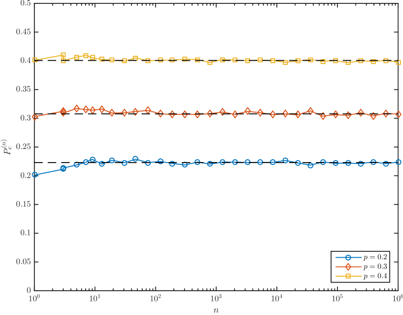
First for the i.i.d. (empty graph) case, Fig. 3 illustrates the detection error probability Pe(n)superscriptsubscript𝑃𝑒𝑛P_{e}^{(n)} versus user size n𝑛n, for several cross-over probabilities p𝑝p. The horizontal lines denote the limit in Proposition 1. It can be seen that Pe(n)superscriptsubscript𝑃𝑒𝑛P_{e}^{(n)} tends to the positive constant given in Proposition 1.
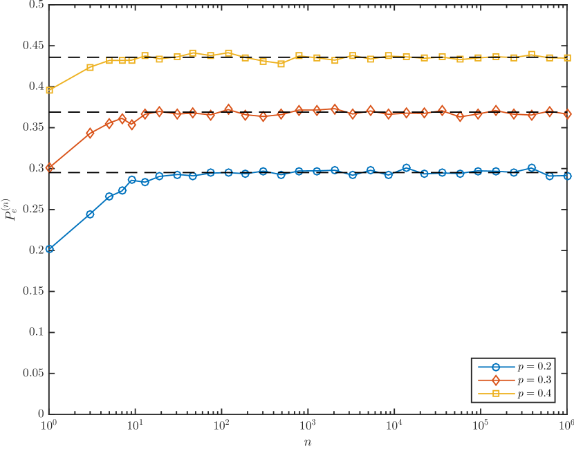
Refer to caption

Figure 3: Pe(n)superscriptsubscript𝑃𝑒𝑛P_{e}^{(n)} v.s. n𝑛n in i.i.d. (empty graph) case.

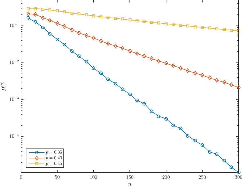
Next for the complete graph case, Fig. 4 illustrates Pe(n)superscriptsubscript𝑃𝑒𝑛P_{e}^{(n)} v.s. n𝑛n for several cross-over probabilities p𝑝p: Fig. 4(a) with θ=0.3𝜃0.3\theta=0.3 corresponds to part (a) of Proposition 3, where the detection error probability tends to the positive constant given there; Fig. 4(b) with θ=0.7𝜃0.7\theta=0.7 corresponds to part (b) of Proposition 3, where the error probability decays to 00 exponentially fast.

Refer to caption
(a) θ=0.3𝜃0.3\theta=0.3
Refer to caption
(b) θ=0.7𝜃0.7\theta=0.7
Figure 4: Pe(n)superscriptsubscript𝑃𝑒𝑛P_{e}^{(n)} v.s. n𝑛n in complete graph case.

VI Conclusion

In this paper, we have analyzed the asymptotic performance of majority sentiment detection in online social networks, and revealed that the detection error probability of a majority sentiment detector is strongly related to the network connections. In the i.i.d. case, where users are not connected, the error probability never reduces to zero, regardless of how large the user base is. This result is interesting in its own right, since one would naively expect the error probability to decay to zero with increasing number of users. Furthermore, by modeling the underlying social network as an Ising Markov random field prior, we discovered an interesting phenomenon of phase transition: in the complete graph case, which is an example of a highly connected network, there exists a critical connection strength. If the strength is below this critical value, the error probability is asymptotically positive, while above this critical value, the error probability tends to zero as the number of users increases. This phase transition seen in the complete graph case is analogous to the critical temperature in statistical physics, which separates the paramagnetic phase, where atom magnetic spins are disordered, from the ferromagnetic phase, where the spins are predominantly in one direction resulting in a magnet. We remark that this phenomenon in the OSN model is not due to the type of detector used - but rather is due to the inherent similarity of opinions among users produced by the network model.

References

  • [1] Philip N Howard and Muzammil M Hussain. Democracy’s fourth wave?: digital media and the Arab Spring. Oxford University Press on Demand, 2013.
  • [2] Efthymios Kouloumpis, Theresa Wilson, and Johanna D Moore. Twitter sentiment analysis: The good the bad and the omg! Icwsm, 11:538–541, 2011.
  • [3] Mike Thelwall, Kevan Buckley, and Georgios Paltoglou. Sentiment in twitter events. Journal of the American Society for Information Science and Technology, 62(2):406–418, 2011.
  • [4] Walter Lippmann. Public opinion. Transaction Publishers, 1946.
  • [5] Peter J Coughlin. Probabilistic voting theory. Cambridge University Press, 1992.
  • [6] Bo Pang and Lillian Lee. Opinion mining and sentiment analysis. Foundations and trends in information retrieval, 2(1-2):1–135, 2008.
  • [7] Rohit Negi, Vinay Uday Prabhu, and Miguel Rodrigues. Latent sentiment detection in online social networks: A communications-oriented view. In Communications (ICC), 2014 IEEE International Conference on, pages 3758–3763. IEEE, 2014.
  • [8] K Binder. Ising model. Hazewinkel, Michiel, Encyclopedia of Mathematics. Springer, 1, 2001.
  • [9] Richard M Dudley. Real analysis and probability, volume 74. Cambridge University Press, 2002.
  • [10] P Pfeuty. An exact result for the 1d random ising model in a transverse field. Physics Letters A, 72(3):245–246, 1979.
  • [11] Martin Kochmański, Tadeusz Paszkiewicz, and Sławomir Wolski. Curie–weiss magnet?a simple model of phase transition. European Journal of Physics, 34(6):1555, 2013.
  • [12] George Pólya and Gabor Szegö. Problems and Theorems in Analysis II: Theory of Functions. Zeros. Polynomials. Determinants. Number Theory. Geometry. Springer Science & Business Media, 1997.