Day of the week effect in
paper submission/acceptance/rejection to/in/by
peer review journals.
II. An ARCH econometric-like modeling
- : ma683@le.ac.uk
2GRAPES111Group of Researchers for Applications of Physics in Economy and Sociology , rue de la Belle Jardiniere 483,
B-4031, Angleur, Belgium
- : marcel.ausloos@ulg.ac.be
3 Institute for the Application of Nuclear Energy (INEP), University of Belgrade, Banatska 31b, Belgrade-Zemun, Serbia
- : olgica@inep.co.rs
4 Institute of Chemistry, Technology and Metallurgy, Department of Electrochemistry, University of Belgrade, Njegoseva12, Belgrade, Serbia
- : dekanski@ihtm.bg.ac.rs
5Faculty of Physics, Warsaw University of Technology,
Koszykowa 75, PL-00-662, Warsaw, Poland
∗ - : mrow@if.pw.edu.pl
∗∗ - : fronczak@if.pw.edu.pl
∗∗∗ - : agatka@olimp.if.pw.edu.pl )
Abstract
This paper aims at providing a statistical model for the preferred behavior of authors submitting a paper to a scientific journal. The electronic submission of (about 600) papers to the Journal of the Serbian Chemical Society has been recorded for every day from Jan. 01, 2013 till Dec. 31, 2014, together with the acceptance or rejection paper fate. Seasonal effects and editor roles (through desk rejection and subfield editors) are examined. An ARCH-like econometric model is derived stressing the main determinants of the favorite day-of-week process.
Keywords :scientific agent behavior; paper submission day; ARCH modeling; seasonal editor effect; acceptance or rejection rate
1 Foreword
Quantitative considerations on human aspects of synchronized behavior or cyclic rhythms are abundant: e.g., menstruation or heart beat [1] - [4]; specific days of week effects are reported for many issues: birth rates, judges’ decisions, car accidents, thieves activity, hospital admission, mortality rate, or when women are feeling to be least attractive [5] - [11] ; for financial markets [12] - [19] a day-of-the-week effect is very well known. Of course, on all such findings, we are aware that statistical critiques are numerous.
In order to acquire information, intended to monitor (hidden) psychological motivations, it is of interest to focus some attention on similar questions outside the financial and economic sphere. There are many possible cases [4], but the data must be first realistically obtained, next it should be reliable, and in fine has to suggest more investigations within a broadening concern about human behavior.
We have been fortunate to get access to such data about submitted, accepted or rejected papers in the peer review process of the Journal of the Serbian Chemical Society (JSCS). We have examined such data in [20]. A behavioral hypothesis about submitting authors was sketched. However, as mentioned by reviewers and others, there was no subsequent model ”describing” the findings. Nevertheless, the outlined hypothesis, based on some expected behavior(s) of scientists, taking into account their work environment, seemed reasonable, suggesting mutatis mutandis some universal feature for when manuscripts are submitted to a journal [20], related to the paper quality influencing editors and reviewers appreciation, whence leading to acceptance or rejection.
However, to propose a behavioral model is not a trivial or common feature when physics rigor is expected. One may mention work in sociophysics [21, 22, 23], but the pertinence of such models can be debated, because of external factors, as pointed for example in [24, 25] and because it is unclear that collective (herding) causes are the primary source of behaviors. The matter is delicate. We understand that models which intend to capture reality through fitting parameters are much scorned upon in physics realms. However, regression models may also present some interest in order to emphasize significant variables [5]. Here below, we propose such a model, based on econometrics technique.
2 Introduction
A peer-review process starts when a paper is submitted to a journal and ends when the paper is accepted or rejected for publication. How reviewers behave has already been much studied. The intellectual writing process after compiling measures and their subsequent analysis is also quite studied. However, a major step occurring when presenting research results is far less studied. This is studied here below, - the submission day, together with some practical measure of its consequences: its influence on the acceptance (or rejection) of the manuscript.
Due to electronic submissions nowadays, the submission is quasi entirely managed by an author of the paper. It is logical to admit that the behavior is often influenced by the action of others, but could also be intrinsic due to societal constraints or habits [26]. Beside such a behavioral aspect, it seems of practical interest, for editors, reviewers and publishers, to explore the timely behavior of agents submitting papers in scientific journals and the editor work flow [27]. It is usual to find some information on the date of submission of a paper in recent years on the first page of a paper. The date of acceptance is also often announced, but the latter depends on many individual factors, inherent to the editorial peer review and process. What is hardly known is the number of papers which are submitted, - on a given day, whatever their later fate. What is quasi unknown is the number of papers which are rejected, after having been submitted on a given day. These last two numbers of submissions, whence the information on the day of submission are entirely and strictly an author behavioral measure with respect to his/her research work. It is not influenced by reviewers or editors (except maybe for special issues with deadlines). Thus, we stress that even though the acceptance or rejection does not entirely depend on the authors, the submission is in his/her hands only.
We have been fortunate to get access to data on submission, acceptance or also rejection from the Journal of the Serbian Chemical Society (JSCS): about 265 papers were accepted along 600 submitted papers over 2 years, i.e. 730 days. The journal contains various sub-sections. It had an impact factor = 0.912 in 2012, - before the years 2013 and 2014, those in which the peer review starting days are examined below. N.B. One might contrast these quantities with the order of magnitude known for another respected journal, Nature which recently reported 3089 of submissions over 10 weeks; this means about 310 papers per week. Only 4 articles and 13 letters were published, e.g., in one of the latest issues. This means a 4% acceptance rate (or 96% rejection rate) [20]. However, we stress that Nature and other journals have not released, to our knowledge, any information neither on the day of submission nor on the fate of the manuscript according to such a day of submission. Therefore our JSCS data present unique features.
We find that, in the JSCS case at hands, more papers are submitted on Wednesday, but when examining the relative acceptance rate, with respect to the total number of submitted papers in a given week day, more papers are accepted for publications if submitted on Tuesday. There is no information on the day of acceptance or rejection by an editor. Only the submission and paper fate process are thus considered as the dependent variables.
To develop a behavioral (agent based-like) model seems too audacious. Let it be observed that what is presently examined is not the peer review process per se, for which several physics-based models have been already outlined, mainly stressing either the editor side [28] or the reviewer side [29, 30], or both [27]. A ”weaker” approach, like a statistical modeling, can be envisaged, as in econometrics: an ARCH-like modeling [16], [31]-[34], - here emphasizing the authors preferred day of submission as well as the most successful day of submission for paper acceptance. We consider that we may take the same modeling approach used to describe an investor behavior differences (on Monday and Friday with respect to other days of the week),
Time series are shown in Sect. 3. A statistical analysis of the daily distributions is briefly recalled for completeness and coherence, repeating some information but also developing on [20]. in Sect. 4; correlations in daily submissions are examined in Sect. 5 in order to search for hidden structure as through ”well known” but unusual distributions (Sect. 4.2). An interference due to the editor role is discussed in Sect.5.1. A possible seasonal influence is examined in Sect. 5.2. A Granger causality test is also performed (Sect. 5.3). Since ARCH and generalized ARCH models might be unfamiliar to readers, in Sect. 6.1, we explain the technical method leading to an ARCH econometric-like model. In Sect. 6.2, we interpret the model parameters and findings through the author’s role at the manuscript submission time. The final section (Sect. 7) re-emphasizes that the role of authors is the primary concern, their behavior extracted from the data through an original modeling process.
3 Data
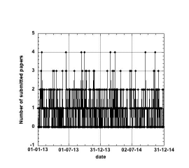
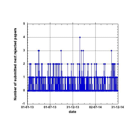
Let us call the number of submitted paper on one given day, the later accepted papers () and those later rejected (). (N.B. In Table 1, , because a few (4) papers were withdrawn by authors.) The submission time series daily records are shown in Fig. 1. It can be mentioned that the periodogram gives a (huge) peak near 0.143 (). A similar graph could be displayed for , but is not shown for saving space. In fact, the latter could be also uploaded for any other journal on internet. Recall that the number of submitted and the number of rejected papers are not usually known (though see [35, 36], in cases concerned with seasonal effects). Therefore, and furthermore in view of the following discussion, it is original to display the time series for the number of rejected papers when submitted on a given day. This is found in Fig. 2.
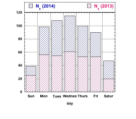
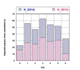
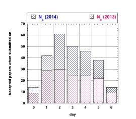
The histogram of the number on a given week day is shown in Fig. 3, emphasizing both years of interest. The corresponding histograms for the number of submitted next either rejected or accepted papers are given in Figs. 4 - 5 respectively.
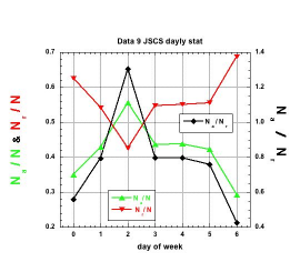
The relative number (expressed in percentages) of papers accepted or rejected after submission ( and ) on a specific day of the week is given in Table 1. The proportion of (i) accepted to submitted papers (), (ii) rejected to submitted papers (), and (iii) accepted to rejected papers (), according to the day-of-the-week is shown in Fig. 6. The ratio of accepted to rejected papers () according to the week day of submission to JSCS in 2013 and 2014 is also shown. The latter number can of course be greater than unity. This occurs on Tuesday.
Thus, it appears that, in contrast to the more often occurring submission day (Wednesday, weekday 3), - see Fig. 3, the papers are (relatively with respect to the number of those submitted on the day) more often accepted when (or if) submitted on Tuesday (day 2). However, the largest number of rejected papers are those submitted on Wednesday (day 3), - see Fig. 4. When expressed in relative terms (in percentages of the submitted papers), - unexpectedly, the greatest proportion of manuscripts gets rejected if they have been submitted on Sunday (day 0) or Saturday (day 6).
| Min | 0 | 0 | 0 | 0 | 0 | 0 | 0 |
| Max | 4 | 3 | 4 | 1 | 1 | 3 | 3 |
| Sum | 597 | 265 | 328 | 177.08 | 212.92 | 102.67 | 97.833 |
| Mean | 0.818 | 0.363 | 0.449 | 0.243 | 0.292 | 0.141 | 0.134 |
| Std Dev | 0.921 | 0.594 | 0.678 | 0.391 | 0.420 | 0.402 | 0.387 |
| Std Err | 0.0341 | 0.0220 | 0.0251 | 0.0145 | 0.01552 | 0.0149 | 0.0143 |
| Skewn | 0.9788 | 1.4865 | 1.4686 | 1.1808 | 0.9093 | 3.1567 | 3.3830 |
| Kurt | 0.457 | 1.522 | 1.935 | -0.3457 | -0.969 | 10.694 | 13.585 |
| 63.92 | 50.884 | 25.244 | [2013-2014] | ||||
| 35.127 | 21.524 | 17.414 | [2013] | ||||
| 32.365 | 36.00 | 14.545 | [2014] | ||||
4 Discussion of the Statistical Daily Distributions
Next, it appears to be of interest to verify whether these visual findings are statistically sound: a value is naturally in order, - see Sect. 4.1. Next, in order to introduce an econometric-like, statistical, modeling, a test on the Weibull distribution seems appropriate, - see Sect. 4.2.
4.1 uniform distribution test
The -test can only be made on the number of papers; assuming a uniform daily distribution, one obtains values given on the last line of Table 1. They range from till . Recall that the value at 0.95% confidence is 18.5476 for 6 degrees of freedom, for a uniform distribution thereby indicating that the submission distribution is far from uniform, i.e. there are significant differences about the day-of-the-week. There is a markedly significant propensity to submit on Wednesday (3rd day-of-the-week). The same conclusion can de drawn about the going-to-be accepted papers. The later rejected papers are more uniformly distributed over the week, - when the yearly distributions are considered. However, when increasing the time range, the -test leads to a value, indicating a non-uniform distribution, in agreement with the visual perception of the Fig. 4 data.
Notice that the distributions are rather skewed and the skewness positive; the statistical characteristics are found in Table 1; the kurtosis is also negative. However an asymmetry holds both for the absolute values and for the percentages; for these the kurtosis is negative. Thus, the characteristics of the various distributions have next been examined in order to search whether they belong to a known case.
4.2 Other shape distribution tests
Searching for the distribution shape, the Weibull probability [37] was first considered; it was originally imagined for survival measures, - of humans or electro-mechanical goods. The Weibull failure model has also been applied in econophysics, for example, when kinds of ”first passage processes” are relevant. Mutatis mutandis, it can be imagined that scientific papers are analog to light bulbs: the former survive if they are published, or die if they are rejected. They might be submitted and accepted elsewhere, of course. We have performed a regression analysis for a ”survival model” assuming that ”failure occurrences” have a Weibull distribution. By extension, we have also tested the Weibull distribution function on the submitted and later accepted papers.
The probability plot correlation coefficient [38] is a graphical technique for identifying the shape parameter for the distributional family that best describes the data set. Such a coefficient has been looked for the 3 distributions (, , and ), for the years 2013 and 2014 and for the whole time interval [2013–2014]. The plots are not ”spectacular” and are not shown for saving space. The optimal shape parameter is always found to be equal to 1, and exponentially decaying when increasing the number of shape parameters, suggesting that the Weibull distribution can be adequate, - among the simplest usually considered. Yet, the skewness and kurtosis seem ”large” (see Table 1), demanding to further examine whether the ”simplicity” of the distributions is so well demonstrated.
The maximum likelihood estimation is another accurate and easy way to estimate distribution parameters [39]. The corresponding plots for papers submitted and those subsequently accepted or rejected on a given day present some structure. The plots (not shown for saving space) do not support normality, but the change in curvature (near ) and the curvature sign allow to infer that the underlying distribution has a tendency toward a so called heavy tail,- whence suggesting a non dubious day effect, but hardly indicating a ”classical distribution”. We are aware that the number of days in a week barely covers one decade, - whence log-log plots for discovering the tail exponents appear to be rather meaningless and are thus not shown.
Tukey tests [40] have also been performed: the resulting values do not point to any of the most usual distribution functions of random events; the distributions are found to be rather far from ”exactly uniform”.
In conclusion of this subsection, it can be considered that the various day-of-the-week distributions do not correspond to a usually well known distribution.
5 Correlations in Daily Submissions
Before attempting an econometric-like regression model, it is necessary to appreciate the relevant variables. One could consider that the editor has a prominent role in rejecting papers, - at least, desk rejected ones. However, there is no information on whether an editor does desk reject a paper on the submission day (or exactly on the corresponding day of submission in another week). A priori, there should be no correlation between the day of submission and the day of desk rejection, since we hypothesize that the rejection follows a lack of quality of a paper because submitted on a given day. Nevertheless some editor role is briefly discussed in Sect. 5.1. In the same spirit, one may wonder whether a seasonal effect can be observed. Indeed most submitted papers are by authors belonging to some university or research laboratory. An academic time effect, related to teaching load, might be searched for. This question is tackled on Sect. 5.2.
5.1 Editor role possible influence
One might argue that the above distributions, in particular those about rejected papers, much depend on reviewers and editors behaviors,- the more so if there are desk rejected papers submitted on days during which the mood or duties of editors is not ”agreeable”. Notice that there were more than a dozen editors during the interval time relevant to this study. Moreover, editors do not necessarily examine submitted papers on the day of submission. It occurred that a few editors were quite responsive, but one case of more than one month ”delay in editor activity” could also been extracted from the data.
The number of desk rejected papers has been mentioned in [20] to be equal to 161. Their day of submission distribution is quasi uniform as depicted in Fig. 4 in [20] and statistically proved through a test corresponding to the 95% confidence of a null hypothesis (uniform distribution) for 6 degrees of freedom. Therefore, the week of day of submission for rejected papers does not seem to be editor dependent, whence allowing us not to consider such a variable for modeling the author behavior and the resulting outcome of his/her submission.
Nevertheless, for completeness, it might be interesting to find out some editorial behavior, through the frequency of desk rejection, in particular the distribution of the day of week when an editor desk reject a paper, whenever the latter has been submitted. In Appendix, it is shown that such a distribution is markedly different from that of the author submission behavior and from that of the distribution of days of submission for rejected papers. This allows us to reject an editorial effect about the submission of papers, and about the outcome (acceptance or rejection) of submitted papers, whence such a variable will not be considered in the following model.
5.2 Possible seasonal influence
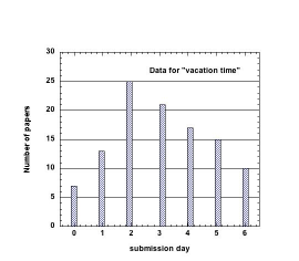
One might argue that authors have a different schedule in the teaching months than during vacation time (say, somewhat arbitrarily between July 01 and August 31). Thus, it may be usefully tested whether the anomalous distribution of submitted papers and of those accepted (or rejected) depends on the year timing. If such a ”teaching duty during academic time” is relevant, it might be expected that the distribution is more uniform during vacation times. We selected the data for those time intervals. The cumulative number of submitted papers for both years on a given day of the week during such so called vacation time (July and August) is shown on Fig. 7. A peak occurs on Tuesday, and a small number of papers is submitted during weekend days. The distribution is visually far from uniform. Thus, it seems apparent that the submission pattern does not depend much on the season, i.e. on academic duties.
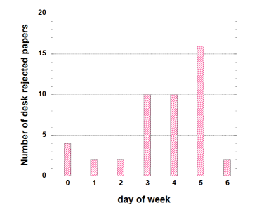
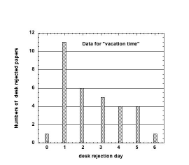
The overall acceptance and rejection fates during vacation time are not examined because they depend on reviewers more than on authors; indeed the paper fate can occur at a later time than July or August. Nevertheless, the desk rejection can be examined to emphasize the editor role, if any, during such a holiday time. This is shown on Fig. 8. As for the academic year, the number of submitted but desk rejected papers increases toward the end of the week. This might imply some effect due to, or correlation with, the mood of editors, during vacation time or before a weekend.
5.3 Granger Causality Test
In view of the above, and with the aim of searching for a model of behavior, one is geared toward further considering the absence of correlations between daily submissions by the different agents. A Granger test of causality seems in order. The Granger causality test is a statistical hypothesis test for determining whether one time series is useful in forecasting another. This is a classical test, for example, systematically applied to the returns on stock indices [41]. Thus, it can be considered as an ad hoc tool for outlining a restricted choice of explanatory variables in the subsequent modeling. The Granger test of causality is based on the vector auto regression (VAR) type regressions, i.e. regression of , i.e. a vector , on its lagged values and the same lags of the , a vector , variable:
| (5.1) |
The null hypothesis corresponds to for all . If so, it means that the does not ”Granger-cause” the variable.
Derived through ”ordinary” least square method (OLS) estimates with robust standard errors, typical results of the Granger causality tests for causality correlations between , , and are given in Table 2, based on F-test statistics values; -values are given.
It can be deduced that the null hypothesis on lack of causality is rejected for all pairs of events with the exception of = f(). The time series are independent of each other (as it should be somewhat expected, it seems). Other time lags have been tested, but have not shown to be carrying any surprising information (bis).
| Model | F | p-value |
|---|---|---|
| = f() | 1.6902 | 0.1082 |
| = f() | 0.3999 | 0.9026 |
| = f() | 0.6622 | 0.7042 |
| = f() | 0.4493 | 0.8709 |
| = f() | 0.8249 | 0.5667 |
| = f() | 1.8717 | 0.0714 * * * |
6 Daily Submission Econometric-like Modeling
Therefore, this paper adopts the forms of so called strong modeling of the day-of-the-week effects of returns () on a stock market, through the ARCH (Autoregressive Conditional Heteroskedasticity) methodology, but differs in the input time series. For the unfamiliar reader, let it be recalled that in econometrics, a ”weak model” has one dummy variable only, so that the time series regression only compares the significance of different coefficients [31]. For example, , where represents the value of the time series on a given Monday; and are to be determined.
In an econometrics ”strong model”, one compares the difference of return rates on one day with those of the other (four) trading days. For example
| (6.1) |
where the coefficients are the unknowns to be determined. Thus, the day-of-the-week effect in a ”strong test” in econometrics refers to the yield rate in a trading day, searching whether this rate is significantly higher or lower than on any other trading day. In this case, five regression equations, like Eq.(6.1) are written to determine the relative size of the yield rate in any of the (five) trading days [44].
A standard OLS method is used for the regression analysis over the single or multiple virtual variables. In bibliometrics, it seems inconvenient to us ”return” as the appropriate word for measuring the fate of scientific papers. The number of these can hardly be called a ”price”, as on a stock market, - although authors when submitting a paper, in some sense, try ”to sell” it to the editor, next to the reviewers, and finally to the community. Thus the analogy with econometrics stops here at the methodology. In brief, the ”short model” will consider one single time series to be regressed through the seven day time series. One will obtain seven coefficients which are to be discussed for observing some significance or not. In contrast, the ”strong model” will consider seven reduced time series, - each one being the original time series measured with respect to the average number (in the appropriate time interval) of submissions in one of each day of the week.
6.1 ARCH-like model
| [day time series] | |||||||
| [2013-2014] | |||||||
| 0 | 0.0000 | -0.5664 | -0.6525 | -0.7381 | -0.5664 | -0.4896 | -0.0768 |
| 1 | 0.5664 | 0.0000 | -0.0861 | -0.1717 | 0.0000 | 0.0768 | 0.4896 |
| 2 | 0.6519 | 0.0860 | -0.0000 | -0.0855 | 0.0860 | 0.1628 | 0.5752 |
| 3 | 0.7374 | 0.1715 | 0.0855 | -0.0000 | 0.1715 | 0.2483 | 0.6607 |
| 4 | 0.5664 | 0.0000 | -0.0861 | -0.1717 | 0.0000 | 0.0768 | 0.4896 |
| 5 | 0.4896 | -0.0768 | -0.1629 | -0.2485 | -0.0768 | -0.0000 | 0.4128 |
| 6 | 0.0768 | -0.4896 | -0.5757 | -0.6613 | -0.4896 | -0.4128 | 0.0000 |
| [2013] | |||||||
| 0 | -0.0000 | -0.5952 | -0.5561 | -0.6912 | -0.5376 | -0.5376 | 0.0960 |
| 1 | 0.5952 | 0.0000 | 0.0391 | -0.0960 | 0.0576 | 0.0576 | 0.6912 |
| 2 | 0.5579 | -0.0392 | 0.0000 | -0.1356 | 0.0185 | 0.0185 | 0.6542 |
| 3 | 0.6912 | 0.0960 | 0.1351 | -0.0000 | 0.1536 | 0.1536 | 0.7872 |
| 4 | 0.5376 | -0.0576 | -0.0185 | -0.1536 | 0.0000 | 0.0000 | 0.6336 |
| 5 | 0.5376 | -0.0576 | -0.0185 | -0.1536 | 0.0000 | 0.0000 | 0.6336 |
| 6 | -0.0960 | -0.6912 | -0.6520 | -0.7872 | -0.6336 | -0.6336 | -0.0000 |
| [2014] | |||||||
| 0 | 0.0000 | -0.5376 | -0.7488 | -0.7861 | -0.5952 | -0.4416 | -0.2496 |
| 1 | 0.5376 | 0.0000 | -0.2112 | -0.2485 | -0.0576 | 0.0960 | 0.2880 |
| 2 | 0.7488 | 0.2112 | 0.0000 | -0.0373 | 0.1536 | 0.3072 | 0.4992 |
| 3 | 0.7887 | 0.2493 | 0.0375 | 0.0000 | 0.1915 | 0.3457 | 0.5383 |
| 4 | 0.5952 | 0.0576 | -0.1536 | -0.1909 | 0.0000 | 0.1536 | 0.3456 |
| 5 | 0.4416 | -0.0960 | -0.3072 | -0.3445 | -0.1536 | 0.0000 | 0.1920 |
| 6 | 0.2496 | -0.2880 | -0.4992 | -0.5365 | -0.3456 | -0.1920 | 0.0000 |
| [day time series] | |||||||
| [2013-2014] | |||||||
| 0 | -0.0000 | -0.2688 | -0.4456 | -0.3600 | -0.2880 | -0.2304 | -0.0000 |
| 1 | 0.2688 | -0.0000 | -0.1768 | -0.0912 | -0.0192 | 0.0384 | 0.2688 |
| 2 | 0.4452 | 0.1767 | -0.0000 | 0.0855 | 0.1575 | 0.2150 | 0.4452 |
| 3 | 0.3597 | 0.0912 | -0.0855 | 0.0000 | 0.0720 | 0.1295 | 0.3597 |
| 4 | 0.2880 | 0.0192 | -0.1576 | -0.0720 | -0.0000 | 0.0576 | 0.2880 |
| 5 | 0.2304 | -0.0384 | -0.2152 | -0.1296 | -0.0576 | 0.0000 | 0.2304 |
| 6 | -0.0000 | -0.2688 | -0.4456 | -0.3600 | -0.2880 | -0.2304 | -0.0000 |
| [2013] | |||||||
| 0 | -0.0000 | -0.3840 | -0.3923 | -0.2880 | -0.2880 | -0.2496 | -0.0000 |
| 1 | 0.3840 | 0.0000 | -0.0083 | 0.0960 | 0.0960 | 0.1344 | 0.3840 |
| 2 | 0.3936 | 0.0084 | 0.0000 | 0.1047 | 0.1047 | 0.1432 | 0.3936 |
| 3 | 0.2880 | -0.0960 | -0.1043 | 0.0000 | 0.0000 | 0.0384 | 0.2880 |
| 4 | 0.2880 | -0.0960 | -0.1043 | 0.0000 | 0.0000 | 0.0384 | 0.2880 |
| 5 | 0.2496 | -0.1344 | -0.1427 | -0.0384 | -0.0384 | -0.0000 | 0.2496 |
| 6 | -0.0000 | -0.3840 | -0.3923 | -0.2880 | -0.2880 | -0.2496 | -0.0000 |
| [2014] | |||||||
| 0 | 0.0000 | -0.1536 | -0.4992 | -0.4315 | -0.2880 | -0.2112 | 0.0000 |
| 1 | 0.1536 | 0.0000 | -0.3456 | -0.2779 | -0.1344 | -0.0576 | 0.1536 |
| 2 | 0.4992 | 0.3456 | -0.0000 | 0.0677 | 0.2112 | 0.2880 | 0.4992 |
| 3 | 0.4329 | 0.2788 | -0.0680 | 0.0000 | 0.1439 | 0.2210 | 0.4329 |
| 4 | 0.2880 | 0.1344 | -0.2112 | -0.1435 | -0.0000 | 0.0768 | 0.2880 |
| 5 | 0.2112 | 0.0576 | -0.2880 | -0.2203 | -0.0768 | 0.0000 | 0.2112 |
| 6 | 0.0000 | -0.1536 | -0.4992 | -0.4315 | -0.2880 | -0.2112 | 0.0000 |
| [day time series] | |||||||
| [2013-2014] | |||||||
| 0 | 0.0000 | -0.3168 | -0.2261 | -0.3782 | -0.2976 | -0.2784 | -0.0960 |
| 1 | 0.3168 | -0.0000 | 0.0907 | -0.0614 | 0.0192 | 0.0384 | 0.2208 |
| 2 | 0.2259 | -0.0906 | -0.0000 | -0.1520 | -0.0714 | -0.0523 | 0.1300 |
| 3 | 0.3779 | 0.0614 | 0.1520 | 0.0000 | 0.0806 | 0.0997 | 0.2820 |
| 4 | 0.2976 | -0.0192 | 0.0715 | -0.0806 | 0.0000 | 0.0192 | 0.2016 |
| 5 | 0.2784 | -0.0384 | 0.0523 | -0.0998 | -0.0192 | 0.0000 | 0.1824 |
| 6 | 0.0960 | -0.2208 | -0.1301 | -0.2822 | -0.2016 | -0.1824 | -0.0000 |
| [2013] | |||||||
| 0 | 0.0000 | -0.2112 | -0.1637 | -0.3648 | -0.2496 | -0.2880 | 0.0960 |
| 1 | 0.2112 | 0.0000 | 0.0475 | -0.1536 | -0.0384 | -0.0768 | 0.3072 |
| 2 | 0.1643 | -0.0476 | -0.0000 | -0.2017 | -0.0861 | -0.1247 | 0.2606 |
| 3 | 0.3648 | 0.1536 | 0.2011 | -0.0000 | 0.1152 | 0.0768 | 0.4608 |
| 4 | 0.2496 | 0.0384 | 0.0859 | -0.1152 | 0.0000 | -0.0384 | 0.3456 |
| 5 | 0.2880 | 0.0768 | 0.1243 | -0.0768 | 0.0384 | -0.0000 | 0.3840 |
| 6 | -0.0960 | -0.3072 | -0.2597 | -0.4608 | -0.3456 | -0.3840 | 0.0000 |
| [2014] | |||||||
| 0 | -0.0000 | -0.4224 | -0.2880 | -0.3931 | -0.3456 | -0.2688 | -0.2880 |
| 1 | 0.4224 | 0.0000 | 0.1344 | 0.0293 | 0.0768 | 0.1536 | 0.1344 |
| 2 | 0.2880 | -0.1344 | -0.0000 | -0.1051 | -0.0576 | 0.0192 | -0.0000 |
| 3 | 0.3944 | -0.0294 | 0.1054 | 0.0000 | 0.0476 | 0.1247 | 0.1054 |
| 4 | 0.3456 | -0.0768 | 0.0576 | -0.0475 | -0.0000 | 0.0768 | 0.0576 |
| 5 | 0.2688 | -0.1536 | -0.0192 | -0.1243 | -0.0768 | 0.0000 | -0.0192 |
| 6 | 0.2880 | -0.1344 | -0.0000 | -0.1051 | -0.0576 | 0.0192 | -0.0000 |
The ”modeling” starts from 7 equations, each left hand side being a time series describing the number of events (which has occurred on a given day). Under a matrix equation form, the system of equations reads
| (6.2) |
where is a (vector) time series and the corresponding average value of an event (in the appropriate time interval), both for some (the same) given week day; is a ( x ) rectangular matrix defining the day when an event occurred, while the vector is supposed to be a white noise; the (7) components of the vector have to be determined. In scalar notations, one has
| (6.3) |
where denotes the successive days in the time series: in our case where = 730 days in 2013-2014, but 365 days in either 2013 or 2014. The index indicates the day of the week: . In other words,
| (6.4) |
where, for example, is a vector which has components equal to 1 each Sunday of the interval and 0 otherwise. The best estimation for the regression parameters holds through the Ordinary Least Squares method for the sum of the ”error” squares:
| (6.5) |
minimizing with respect to , i.e. let the first derivative equal to 0, one gets:
| (6.6) |
where is the transposed of .
The coefficients of the submission time series are given for each year of interest and (for comparison) for the whole time interval in Table 3. The corresponding values of the papers submitted on a given day and either (later) accepted or (later) rejected are given in Table 4 and Table 5, respectively. The data is given with 4 decimals: the last one points to the (expected) precision in the regression parameter estimation. For the reader’s ease, let it be made clear that, for example, the value , in Table 3, corresponds to in Eq.(6.4). The matrix of ’s as given in the Tables is of course antisymmetric, whence the ”diagonal” has 0. Sometimes outside the ”diagonal”. This is a consequence of the fact that the mean number of events occurs to be the same on two different days. The sign indicates whether the contribution is ”positive” or ”negative” with respect to the mean of the day. It can be noticed that the sign can change from a time interval to another, but this (of course) only occurs for small values of .
The differences between the various ’s indicate the relevance of a week day with respect to another one. Recall that if is significantly different from 0, it can be considered that the event (”yield rate” in econometrics) is significant as compared with the other days, namely there is an ”effect” on a given day, - due to activity (or lack of activity) in other days. Visually, the relevance of the days in the middle of the week is noticeable and well reproduced for the submission and (later) acceptance of papers. In contrast, the most likely rejection of papers submitted on the weekend is less systematic. This mathematically illustrates the skewed distribution shown and seen in Fig. 4.
6.2 Reasoning
Recall that we propose the alternative to the null hypothesis about the significance of days of submissions of papers submitted to a scientific journal. We propose that the quality of submitted papers is somewhat reflected through the day of submission.
-
•
Indeed, it can be conjectured that researchers who submit on Saturday or Sunday do so because they want top get rid of papers; some pressurizing coauthor or themselves expect the manuscript to have been sent by Friday. Maybe, these scientists are less eager to read very carefully once again their manuscript or are less inspired to redraw conclusions or to demonstrate significant relations in the results or to report to their boss that ”things” have not yet been finalized.
-
•
A comment on the ARCH regression model is in order here in view of distinguishing it from ”agent based models”. By analogy with econometric forecasters who have found some possibility to predict future variations, it can be immediately suggested that the ARCH model provides one way of forecasting submission variance change over time, outside (or beyond) the usual Markov memory free process. Thus, this type of statistical model has a variety of characteristics which should make it attractive for bibliometrics and scientometrics applications, but also allow technological means of artificial intelligence for helping editors [27].
Nevertheless, the ARCH model can be criticized because it assumes that the variance does not change with time. However, this does not seem to be a strong assumption here. Indeed one can verify that the [2013-2014] variance = 0.8488, while the [2013] and [2014] are respectively equal to 0.8933 and 0.7976, - for submitted manuscripts on a given day. In order to take into account a time dependent variance, a GARCH model [45] would be in order, but this is outside the scope of the present paper.
7 Conclusion
First, in summary, there is quite a number of studies on the ”day-of-the-week” effect on financial markets. To the best of our knowledge, this is the first time that one quantifies the submission of scientific papers, thus the behavior of scientific agents in such a process, i.e. considering some author’s brain work and scientific activity content, depending on the day-of-the-week. It has been shown that the analysis should take into account the relative size of daily submissions within a week. This normalization is relevant in order to observe whether the acceptance and rejection rates will differ depending on the day of submission. In view of the high relative independence of scientific agents submitting papers, a statistical analysis of the submission time series is the most appropriate one. This has been attempted through an econometric formulation like the ARCH model.
Interestingly, since the available data gives some information on the fate of each submitted paper, acceptance or rejection, these two time series have been statistically and ”econometrically” analyzed. It is concluded that in the examined case, there is a significant middle of the week effect, not only for the submission, but also for the acceptance rate. It is surmised that the quality of submitted papers varies with the day of submission. Some explanation of the finding is given in terms of stress and collective pressure. It is true that such a hypothesis would be better confirmed if a study of the number of authors and their expertise level was added to the analysis. This would be an easy addition of a couple terms (”variables”) in the ARCH modeling, but the matter falls far outside the present aims.
Within the present framework and methodology, another aspect could be interestingly examined, i.e. the ”relative time series”: , , and . Indeed the conclusion based on absolute numbers and relative numbers could be debated, - the more so depending on the denominator in an expression ”relative to what”. Thus, an ARCH modeling of percentages might allow some further discrimination in the relative importance of the correlations in the day-of-the week effect.
In conclusion, let us to offer a few suggestions for further research lines, first based on possible ”ambiguities” in our findings. It would be interesting to see: (i) whether there is a general trend in authors’ behavior when choosing the submission day of the week and (ii) whether the final decision on the paper exhibits a similar relation to the day of submission in other types of scientific papers. According to our results, it seems that weekend days (Saturday and Sunday) are not the best time for finalizing and submitting manuscripts. We have been intrigued to see how many papers are desktop rejected. The role of editor does not seem to be stochastic; it confirms the hypothesis that the apparent quality of a paper depends is correlated to the day of submission.
Of course, we admit that the fate of a manuscript depends on many peer review process participants, beside the authors, [46], namely editors and reviewers [47]. In order to reveal (possible) ”day-of-the-week” effect in the entire process of scientific publication, it would be of interest to investigate when reviewers are informed that they should review a paper, when they accept (or refuse) to review the submission, when they comment on the paper, etc., but such data for the JSCS are alas not available. However, these data rather pertain to reviewers and editors behaviors, - not to authors, as focussed upon here.
Acknowledgements
This paper has been part of scientific activities in COST Action TD1306 New Frontiers of Peer Review (PEERE).
MA thanks Sonia Bentes, Roy Cerqueti, Claudiu Herteliu, Bogdan V. Ileanu, and Claudio Lupi for comments and advices on the ARCH methodology.
MM, PF, and AF were supported by internal funds of the Faculty of Physics at Warsaw University of Technology.
Appendix
Note on the day of desk rejection
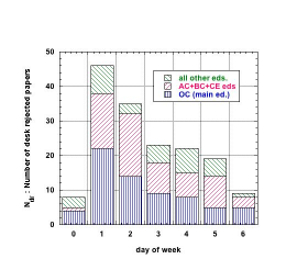
In this Appendix, we examine the editorial behavior with respect to the rejection of papers. Although it is unlikely that an editor waits an exactly multiple of 7 for examining a submitting paper and desk rejecting it, one might in so doing observe when editors are more active during specific days of the week or not, and whether their rejection rate has a specific pattern related to the aper submission. In order to do so, we have examined on what day of the week a paper is desk rejected. Of course, this is strictly an editor affair, unknown to the submitting author. For such a query, and display ease, we have made 3 groups of editors among the dozen or so in charge of subfields: the ”main editor” carrying about 40% of the work load, i.e., the so called OC (organic chemistry subfield), the next editors (analytical chemistry, biochemistry, and chemical engineering, - in short AC, BC, and CE subfields), and the other 10 or so editors. The number of desk rejected papers on a given day of the week, whenever the paper was submitted is shown in Fig. 9. It can be observed that the distribution is an exponentially decaying function () of the day of the week, with a ”relaxation time” .
Apparently editors seem very active at the beginning of the week for rejecting papers, we insist, whatever their submission day. It seems that one can be easily convinced that editors (we do not have data for the reviewer recommendation day) are equally moody and fair (or unfair) during the whole week irrespective of the day; see related discussions in [28] and [48]. Thus, such an a posteriori effect, unknown to authors has not to be included in the relevant variables of the model.
This number of desk rejected papers on a given day (Fig. 9) can be usefully compared to data in Fig. 3 and Fig. 4 pertaining to the submission day and rejection fate depending on the submission day. From these, the related percentages can be easily deduced for comparison to data in Fig. 6. This is left for the reader perusal.
For completeness, in so doing adding to the data reported in Sect. 5.2, we also display the number of desk rejected papers by all editors during ”vacation time” on Fig. 10.
A similar exponential-like behavior, as that found in Fig. 9, for the overall editor rejection day distribution, is found with a relaxation time decay . Thus, one can consider that the editors are equally behaving during the academic year or during the vacation time.
Notice that a conclusion based on the data examined in this appendix seems to indicate that editors work much at the beginning of the week.
References
- [1] McClintock, M. K. (1971). Menstrual Synchrony and Suppression. Nature, 229,(5282): 244-245.
- [2] Ivanov, P.Ch., Amaral, L.A.N., Goldberger, A.L., Havlin, S., Rosenblum, M.G., Struzik, Z., & Stanley, H.E. (1999). Multifractality in human heartbeat dynamics. Nature, 399, 461-465.
- [3] Glass, L. (2001). Synchronization and rhythmic processes in physiology. Nature, 410, 277-284.
- [4] Roehner, B.M. (2007). Driving forces in physical, biological and socio-economic phenomena: a network science investigation of social bonds and interactions (Cambridge University Press).
- [5] Herteliu, C., Ileanu, B.V., Ausloos, M., & Rotundo, G. (2015). Effect of religious rules on time of conception in Romania from 1905 to 2001. Human Reproduction, 30(9), 2202-2214.
- [6] Danziger, S., Levav, J. & Avnaim-Pesso, L. (2011). Extraneous factors in judicial decisions. Proc. Natl Acad. Sci. USA, 108(17), 6889–6892; ibid. 108(42), E834.
- [7] Pigman, J.G. , Rizenbergs, R. L., & Herd, D.R. (1978). Analysis of Weekday, Weekend, and Holiday Accident Frequencies. Research Report No. 513, Division of Research, Bureau of Highways, Department of Transportation, Commonwealth of Kentucky.
- [8] Ryan, K., Levit, K., & Davis, P.H. (2010). Characteristics of Weekday and Weekend Hospital Admissions. Statistical Brief #87, US Agency for Health Care Policy and Research.
- [9] Meacock, R., Anselmi, L., Kristensen, S.R., Doran, T., & Sutton, M. (2016). Higher mortality rates amongst emergency patients admitted to hospital at weekends reflect a lower probability of admission J. Health Serv. Res. Policy . 1355819616649630.
- [10]
- [11]
- [12] French, K.R. (1980). Stock submissions and the weekend effect. Journal of Finance and Economic, 8, 55-69.
- [13] Smirlock, M. & Starks, L. (1986). Day-of-the-week and intra-day effects in stock submission. Journal of Financial Economics, 17,: 197-210.
- [14] Abu Bakar, A., Siganos, A., & Vagenas-Nanos, E. (2014). Does mood explain the Monday effect?. Journal of Forecasting, 33(6), 409-418.
- [15] Rystrom, D.S., & Benson, E.D. (1989). Investor psychology and the day-of-the-week effect. Financial Analysts Journal, 45, 75-78.
- [16] Franses, P.H., & Paap, R. (2000). Modelling day-of-the week seasonality in the S&P 500 index. Applied Financial Economics, 10(5), 483-488
- [17] Berument, H., & Kiymaz, H. (2001). The day of the week effect on stock market volatility. Journal of Economics and Finance, 25(2), 181–193.
- [18] Kiymaz, H., & Berument, H. (2003). The day of the week effect on stock market volatility and volume: International evidence. Review of Financial Economics, 12(4), 363–380.
- [19] Cellini, R., & Cuccia, T. (2014). Seasonal processes in the Euro-US Dollar daily exchange rate. Applied Financial Economics, 24(3), 161-174.
- [20] Ausloos, M., Nedic, O., &. Dekanski, A. (2016). Day of the week effect in paper submission/acceptance/rejection to/in/by peer review journals. Physica A 456, 197-203.
- [21] Galam, S. & Moscovici, S. (1991). Towards a theory of collective phenomena: consensus and attitude changes in groups. European Journal of Social Psychology, 21(1) 49–74.
- [22] Contucci, P. & Ghirlanda, S. (2007). Modeling society with statistical mechanics: an application to cultural contact and immigration Quality & Quantity 41(4), 569–578.
- [23] Ausloos, M. (2013). Another analytic view about quantifying social forces. Advances in Complex Systems 16(1), 1250088.
- [24] Weinshall-Margel K. & Shapard, J. (2011). Overlooked factors in the analysis of parole decisions. Proc. Natl. Acad. Sci. USA, 108 (42), E833.
- [25] Kulakowski, K., Gronek, P., & Dydejczyk, A. (2013). How many parameters to model states of mind? Proceedings 27th European Conference on Modelling and Simulation ECMS Webjorn Rekdalsbakken, Robin T. Bye, Houxiang Zhang (Editors).
- [26] Goodwin, N., Nelson, J.A., Ackerman, F., & Weisskopf, Th. (2004). A Post-Autistic Introduction to Economic Behavior. Post-autistic Economics Review, 28, article 4.
- [27] Mrowinski, M.J., Fronczak, A., Fronczak, P., Nedic, O., & Ausloos, M. (2016). Review times in peer review: quantitative analysis and modelling of editorial workflows, Scientometrics 107, 271-286.
- [28] Wang, W., Kong, X., Zhang, J., Chen, Z., Xia, F., & Wang, X. (2016). Editorial behaviors in peer review. SpringerPlus 5(1), 1–11.
- [29] Thurner, S. & Hanel, R. (2011). Peer-review in a world with rational scientists: Toward selection of the average. The European Physical Journal B 84(4), 707–711
- [30] Kovanis, M., Porcher, R., Ravaud, Ph., & Trinquart, L. (2016). Complex systems approach to scientific publication and peer-review system: development of an agent-based model calibrated with empirical journal data. Scientometrics 106(2), 695–715,
- [31] Bollerslev, T., Engle, R.F., & Nelson, D.B. (1994). ARCH models. Handbook of Econometrics, 4, 2959–3038.
- [32] Aknouche, A., & Bibi, A. (2009). Quasi-maximum likelihood estimation of periodic GARCH and periodic ARMA-GARCH processes. Journal of Time Series Analysis, 30(1), 19-46.
- [33] Cross, F. (1973). The behavior of stock prices on Fridays and Mondays. Financial Analyst Journal, 29(6), 67-69.
- [34] Gibbons, M., & Hess, P. (1981). Day of the week effects and asset returns. Journal of Business, 54, 579-596.
- [35] Bornmann, L. & Daniel, H.-D. (2011). Seasonal bias in editorial decisions? A study using data from chemistry. Learned Publishing 24(4), 3 5–328.
- [36] Schreiber, M. (2012). Seasonal bias in editorial decisions for a physics journal: you should write when you like, but submit in July. Learned Publishing 25(2), 145–151 (2012).
- [37] Sharif, M.N., & Islam, M.N. (1980). The Weibull distribution as a general model for forecasting technological change. Technological Forecasting and Social Change, 18(3), 247-256.
- [38] Filliben, J.J. (1975). The probability plot correlation coefficient test for normality. Technometrics, 17’(1), 111–117;
- [39] NIST/SEMATECH e-Handbook of Statistical Methods, ; MLE 8.4.1.2. Maximum likelihood estimation.
- [40] Tukey, J. (1949). Comparing Individual Means in the Analysis of Variance. Biometrics, 5(2), 99-114.
- [41] Syczewska, E.M. (2014). The EURPLN, DAX and WIG20: The Granger Causality Tests Before and During the Crisis. Dynamic Econometric Models 14, 93-104.
- [42] Wessa P. (2013), Bivariate Granger Causality (v1.0.3) in Free Statistics Software (v1.1.23-r7), Office for Research Development and Education,
- [43] Seth, A.K. (2007). Granger causality. Scholarpedia, 2(7), 1667.
- [44] Brennan, M.J. & A. Subrahmanyam, A. (1996). Market microstructure and asset pricing: On the compensation for illiquidity in stock returns. Journal of Financial Economics, 41(3), 441–464.
- [45] Engle, R. (2001). GARCH 101: The Use of ARCH/GARCH Models in Applied Econometrics. The Journal of Economic Perspectives, 15(4), 157–168.
- [46] Hargens, L.L. (1988). Scholarly Consensus and Journal Rejection Rates. American Sociological Review 53(1), 139-151.
- [47] Ausloos, M., Nedic, O., Fronczak, A., & Fronczak, P. (2015). Quantifying the quality of peer reviewers through Zipf’s law. Scientometrics, 106, 347-368.
- [48] Lortie, Ch.J., Allesina, St., Aarssen, L., Grod, O., & and Budden, A. E. (2013). With Great Power Comes Great Responsibility: the Importance of Rejection, Power, and Editors in the Practice of Scientific Publishing. PloS one 8(12), e85382.