Event-Ready Bell Test Using Entangled Atoms Simultaneously Closing Detection and Locality Loopholes

Abstract

An experimental test of Bell’s inequality allows ruling out any local-realistic description of nature by measuring correlations between distant systems. While such tests are conceptually simple, there are strict requirements concerning the detection efficiency of the involved measurements, as well as the enforcement of spacelike separation between the measurement events. Only very recently could both loopholes be closed simultaneously. Here we present a statistically significant, event-ready Bell test based on combining heralded entanglement of atoms separated by $398\,\mathrm{m}$ with fast and efficient measurements of the atomic spin states closing essential loopholes. We obtain a violation with $S=2.221\pm 0.033$ (compared to the maximal value of $2$ achievable with models based on local hidden variables) which allows us to refute the hypothesis of local-realism with a significance level $P<2.57\cdot 10^{-9}$.

Back in 1935 Einstein, Podolsky and Rosen (EPR) pointed at inconsistencies in quantum mechanics, if one requires that a physical theory has to be realistic and local Einstein et al. (1935). In such theories any signal, influence, or interaction propagates at most at the speed of light (locality), and one can assign properties to quantum systems before a measurement (realism). To achieve the latter, they left open the possibility to complement quantum mechanics with, nowadays called, local hidden variables (LHV). Starting from the EPR example on analyzing measurement results of two independent observers, John Bell showed that the prediction of QM for certain measurement scenarios differ from the prediction of all local, realistic theories Bell (1964). With this he directly provided a prescription for how to evaluate the validity of the EPR claims and of any LHV theory in an experiment.

However, there are stringent requirements on an experimental test, as LHVs give a theory an amazing flexibility to account for observed results. In spite of the many experiments started soon after Bell’s discovery (e.g. Freedman and Clauser (1972); Aspect et al. (1982)), which (almost) all agreed well with QM, they all relied on assumptions on the observers or the observed systems, thus opening loopholes to the LHV theories under test (for reviews see, e.g., Clauser and Shimony (1978); Tittel and Weihs (2001); Larsson (2014)).

One loophole, the locality loophole, concerns the independence of the observers, which only can be warranted if the whole measurement processes of the two observers are spacelike separated. This was achieved by Weihs et al. Weihs et al. (1998), where the whole measurement, starting from the choice of a random number up to the appearance of the classical voltage signal of a single photon detection was outside the light cone of the other measurement. However, as detection of single photons was notoriously inefficient those days, one had to assume fair sampling, i.e. that the registered photon pairs had been a representative sample of all pairs - thus leaving open the so called detection loophole. This was closed for the first time in an experiment using trapped, entangled ions Rowe et al. (2001), which, however, were separated only by few micrometers - leaving the locality loophole open. Since then the goal was to close both in a single experiment, leading to key developments such as the first observations of atom-photon entanglement Blinov et al. (2004); Volz et al. (2006) and atom-atom entanglement over larger distances Moehring et al. (2007); *Ritter2012; Hofmann et al. (2012). Recently, based on electron spins of separated nitrogen-vacancy (NV) centers Jelezko and Wrachtrup (2006) the first experimental test of Bell’s theorem without the locality and detection loophole was performed Hensen et al. (2015). With the development of efficient photon pair sources Fedrizzi et al. (2007); *Trojek2008 and highly efficient single photon detectors Lita et al. (2008) two tests succeeded also with entangled photon pairs Giustina et al. (2015); Shalm et al. (2015).

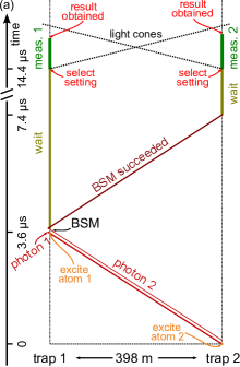
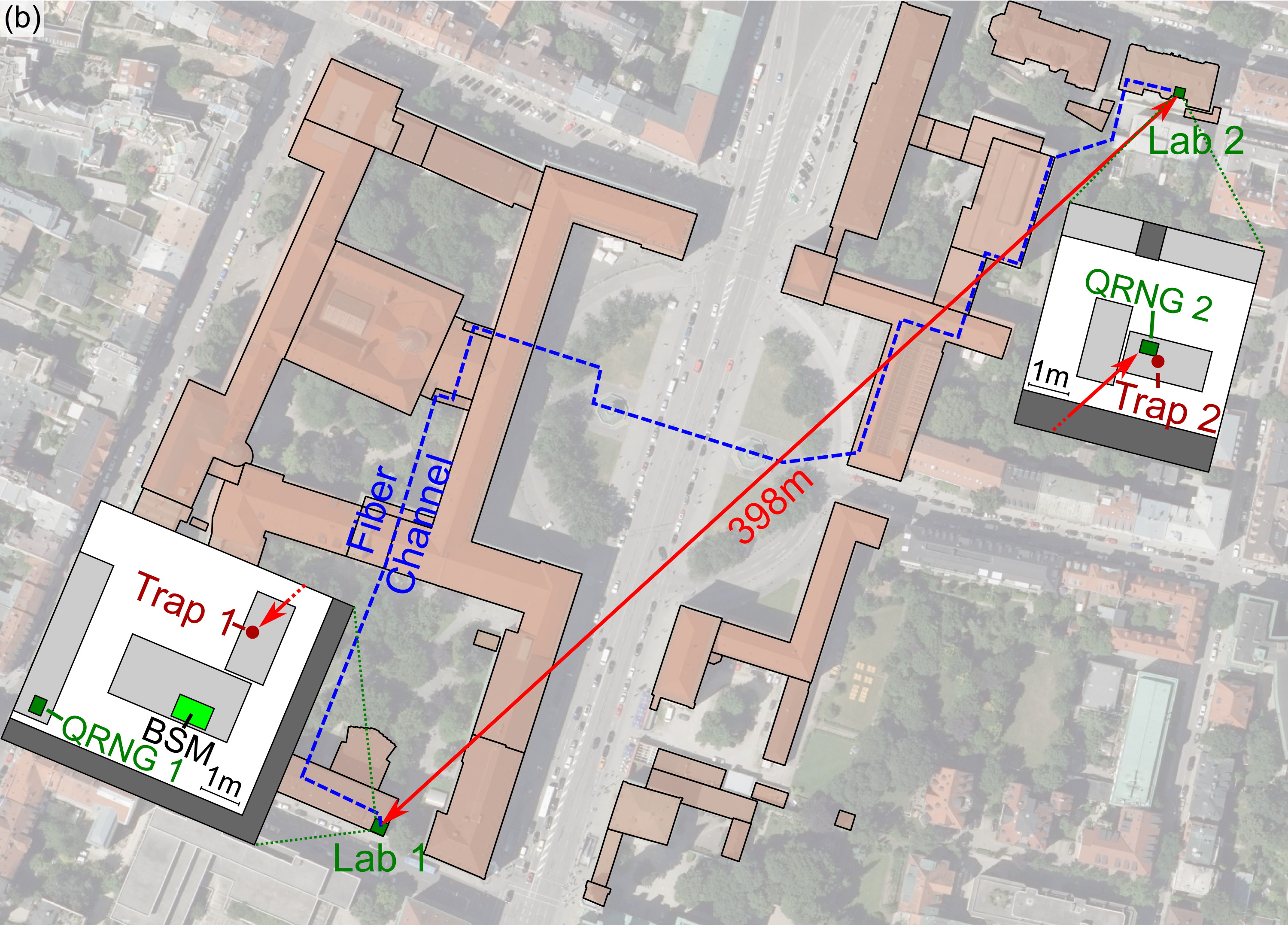
Figure 1: (a) Space-time diagram of the experiment. The two observers (trap 1 and trap 2) are separated by $398\,\mathrm{m}$ with the BSM setup being located close to trap 1. Single photons and all communication signals are transmitted via optical fibers (lengths vary around $700\,\mathrm{m}$) laid in cable ducts connecting the two stations. Sending a photon from trap 2 to the BSM takes roughly $3.6\,\mathrm{\mu s}$ (photons from both traps arrive within a window of $120\,\mathrm{ns}$ represented by two lines for earliest and latest emission). Another $3.7\,\mathrm{\mu s}$ are needed for communicating the success of the BSM back to trap 2. The state measurements (including random choice of the measurement direction) are performed such that a result is obtained outside of the light cone of the other side. (b) Overview of the experimental location on the main campus of LMU. Trap 1 is located in the basement of the faculty of physics and trap 2 in the basement of the department of economics. Map data were provided by ver . BSM: Bell state measurement, QRNG: quantum random number generator.

Here we describe the evaluation of LHV theories using entangled neutral atoms closing both the locality and the detection loophole in a single experiment. Based on atom-photon entanglement, entanglement swapping Zukowski et al. (1993) allowed to prepare in a heralded manner entangled spin states of two atoms separated by a distance of $398\,\mathrm{m}$, well suited for an event-ready test. For an event-ready test no fair sampling assumption has to be made Bell (1988); Zukowski et al. (1993). There a measurement result is reported every time the heralding signal confirming the successful distribution of entanglement to the observers was obtained and thus no detection loophole is opened at all. Any inefficiencies or inaccuracies in the atomic state detection then only influence the degree of achievable correlations. The locality loophole is closed by employing fast and efficient measurements of the atomic spin states at a sufficient distance together with fast quantum random number generators (QRNG) for selection of the measurement basis. We employed state-dependent ionization for highly efficient atomic state analysis and with a total observation time of about a microsecond also the spacelike separation could be warranted. Well-defined hypothesis tests with samples of $10000$ observations clearly indicate that LHV theories do not allow a correct description of nature.

We consider the simplest situation of an event-ready Bell test, where two separate observers are told - according to a heralding signal - to report the result of two-outcome measurements $A$, $B$ $\in\{\uparrow,\downarrow\}$ performed on each side (an example are measurements on spin-$\frac{1}{2}$ particles). For a test of local realism the two observers choose their measurement directions from two possibilities $a\in\{\alpha,\alpha^{\prime}\}$ and $b\in\{\beta,\beta^{\prime}\}$ and afterwards compare their results. For this situation Clauser, Horne, Shimony, and Holt (CHSH) put Bell’s inequality in an experimentally friendly form Clauser et al. (1969):

$$S=\left|\left\langle\sigma_{\alpha}\sigma_{\beta}\right\rangle+\left\langle\sigma_{\alpha}\sigma_{\beta^{\prime}}\right\rangle\right|+\left|\left\langle\sigma_{\alpha^{\prime}}\sigma_{\beta}\right\rangle-\left\langle\sigma_{\alpha^{\prime}}\sigma_{\beta^{\prime}}\right\rangle\right|\leq 2,$$ (1)

with correlators $\left\langle\sigma_{a}\sigma_{b}\right\rangle=\frac{1}{N_{a,b}}(N_{a,b}^{\uparrow\uparrow}+N_{a,b}^{\downarrow\downarrow}-N_{a,b}^{\uparrow\downarrow}-N_{a,b}^{\downarrow\uparrow})$. Here $N_{a,b}^{A,B}$ denote the number of events with the respective outcomes $A$, $B$ for measurement directions $a$, $b$ and $N_{a,b}$ is the total number of events of the respective measurement setting. Quantum mechanics predicts a violation of this inequality when measurements are performed on maximally entangled states $\left|\Psi^{\pm}\right\rangle=\frac{1}{\sqrt{2}}\left(\left|\uparrow\right\rangle\left|\downarrow\right\rangle\pm\left|\downarrow\right\rangle\left|\uparrow\right\rangle\right)$ with certain measurement settings, e.g., $\alpha=0^{\circ}$, $\alpha^{\prime}=90^{\circ}$, $\beta=-45^{\circ}$, $\beta^{\prime}=45^{\circ}$. Angles $\alpha,\beta$ are defined here in the spin space.

In our case the two observer stations are independently operated setups (trap 1 and trap 2) that are equipped with their own laser and control systems. Their separation of $398\,\mathrm{m}$ (Fig. 1) makes $1328\,\mathrm{ns}$ available to warrant spacelike separation of the measurements. On each side we store a single ${}^{87}\mathrm{Rb}$ atom in an optical dipole trap. The employed internal spin states ($\left|\uparrow\right\rangle_{z}$ and $\left|\downarrow\right\rangle_{z}$) are the Zeeman states $\left|m_{F}=+1\right\rangle$ and $\left|m_{F}=-1\right\rangle$ of the ground level $5^{2}S_{1/2}$, $F=1$ (Fig. 2(a)). Entanglement of the atoms is generated by first entangling the spin of each atom with the polarization of a single emitted photon Volz et al. (2006). The photons are guided to an interferometric Bell state measurement (BSM) setup (Fig. 2), located close to trap 1. It consists of a fiber beam splitter (BS) followed by polarizing beam splitters (PBS) in each of the output ports, where detection of photons is performed by four avalanche photodiodes (APDs). This setup allows to distinguish two maximally entangled photon states. Thereby a two-photon coincidence in particular detector combinations (see Sec. I.B of the Supplemental Material sup , which includes Refs. Glauber (2007); Loudon (1997); L’Ecuyer and Simard (2007); Zhang et al. (2013); McDiarmid (1989); Bednorz (2015); Adenier and Khrennikov (2015)) heralds the projection of the atoms onto one of the states $\left|\Psi^{\pm}\right\rangle=\frac{1}{\sqrt{2}}\left(\left|\uparrow\right\rangle_{x}\left|\downarrow\right\rangle_{x}\pm\left|\downarrow\right\rangle_{x}\left|\uparrow\right\rangle_{x}\right)$ Hofmann et al. (2012), where $\left|\uparrow\right\rangle_{x}=\frac{1}{\sqrt{2}}\left(\left|\uparrow\right\rangle_{z}+\left|\downarrow\right\rangle_{z}\right)$ and $\left|\downarrow\right\rangle_{x}=\frac{i}{\sqrt{2}}\left(\left|\uparrow\right\rangle_{z}-\left|\downarrow\right\rangle_{z}\right)$.

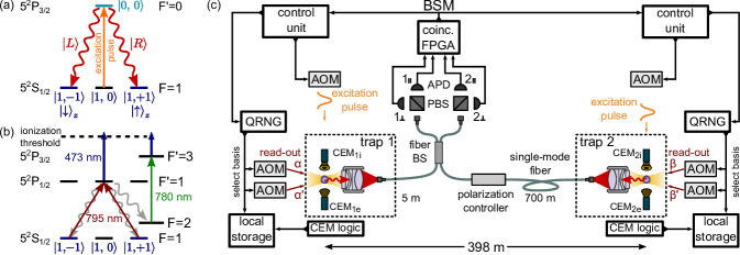
Figure 2: (a) Scheme of the atomic levels involved in the entanglement between the spin state of the atom (subspace $5^{2}S_{1/2}$, $F=1$, $\left|m_{F}=\pm 1\right\rangle$) and polarization of the photon (left- and right-circular, $\left|L\right\rangle$, $\left|R\right\rangle$, respectively). Entanglement is generated in the spontaneous decay of the $5^{2}P_{3/2}$, $F^{\prime}=0$ state after optical excitation. (b) Scheme of the atomic state measurement. A selected superposition of the spin states is excited to the $5^{2}P_{1/2}$, $F^{\prime}=1$ level depending on the polarization of a $795\,\mathrm{nm}$ laser pulse and is ionized with a $473\,\mathrm{nm}$ laser. The atom can spontaneously decay to the $5^{2}S_{1/2}$, $F=1$ or $F=2$ levels during this procedure (gray wavy arrows). While decays into the $F=1$ level can reduce the fidelity of the measurement process, population in the $F=2$ level is excited with an additional $780\,\mathrm{nm}$ laser and ionized as well. (c) Schematic of the experimental setup. In each trap spin-polarization entanglement is generated between the atom and a single photon which is guided to the BSM via a single-mode fiber. Polarization stability in the $700\,\mathrm{m}$ fiber connecting trap 2 and the BSM is ensured by automatic compensation Rosenfeld et al. (2008) performed every $5\,\mathrm{min}$ using reference light and a polarization controller. The photons are overlapped on a fiber beam splitter (BS), their coincident detection heralds entanglement of the atomic spins. Local measurements are performed on the atomic spins according to settings selected by quantum random number generators (QRNGs). AOM: acousto-optic modulator, APD: avalanche photo diode, CEM: channel electron multiplier, FPGA: field programmable gate array, PBS: polarizing beam-splitter.

The experimental sequence (see Supplemental Material sup Sec. I.B for further details) starts after two atoms are loaded into the traps. Photons emitted by the atoms are coupled into optical fibers. The efficiencies for detecting a single photon in the BSM arrangement after excitation in trap 1 or trap 2 are $\eta_{1}=1.65\times 10^{-3}$ and $\eta_{2}=0.85\times 10^{-3}$ (the latter also includes the transmission loss of photons ($\lambda=780\,\mathrm{nm}$) in the $700\,\mathrm{m}$ fiber of approximately $50\%$). This results in an overall probability to obtain a heralding signal in the BSM of $0.7\times 10^{-6}$. If no signal is obtained the excitation sequence of the atoms is repeated. Including times necessary for transmission of signals as well as to prepare and to cool the atoms, the average rate of excitation attempts is $5.2\times 10^{4}\,\mathrm{s^{-1}}$. Depending on the loading rate of the traps this results in about $1$ - $2$ heralding events per minute. The atom excitation procedures are synchronized to $<1\,\mathrm{ns}$ (Supplemental Material sup Sec. I.A) such that the emitted photons entangled with the respective atoms have, at the BSM setup, a temporal overlap close to unity Hofmann et al. (2012).

After a successful BSM signals are sent to both observers where they trigger the switching to atomic state measurement. An additional waiting time has to be introduced due to dephasing and rephasing of atomic states in strongly focused dipole traps. There, longitudinal field components lead to an inhomogeneous light polarization which results in a state- and position-dependent AC Stark shift. Due to the antisymmetry of the polarization distribution this accumulated phase is compensated after one transverse oscillation Rosenfeld (2008); *Thompson2013; *TBP01. To obtain simultaneous rephasing the radial trap frequencies are chosen for an oscillation period $\frac{2\pi}{\omega_{r}}$ of $11.2\,\mu s$ and $14.5\,\mathrm{\mu s}$ for trap 1 and trap 2, respectively, by setting the trap depths. The measurement procedure starts with selecting the analysis direction according to the output of a fast quantum random number generator. As a further development of Fürst et al. (2010) these QRNGs have minimal bias (typ. less than $10^{-5}$) without any postprocessing Abellan et al. (2015). The random bit in trap 1 (trap 2) determining the direction $\alpha/\alpha^{\prime}$ ($\beta/\beta^{\prime}$) is provided on request and has no measurable correlation to bits generated earlier than $80\,\mathrm{ns}$ before, see the Supplemental Material sup Sec. II for details. In the sense of independence to previous information, we thus consider this moment before the request as the starting time of the measurement.

For the analysis of the atomic state a state-selective ionization is employed where the measurement direction $\gamma\in\{\alpha,\alpha^{\prime},\beta,\beta^{\prime}\}$ is determined by the polarization of a readout laser at $795\,\mathrm{nm}$ exciting the atom to the $5^{2}P_{1/2}$, $F^{\prime}=1$ level from where it is ionized by an additional laser at $473\,\mathrm{nm}$ (Fig. 2(b)). In particular, we ionize the state $\left|\uparrow\right\rangle_{\gamma}=\sin(\gamma/2)\left|\uparrow\right\rangle_{x}-\cos(\gamma/2)\left|\downarrow\right\rangle_{x}$ using linear polarization at an angle $\gamma/2$ relative to the horizontal. The state $\left|\downarrow\right\rangle_{\gamma}=\cos(\gamma/2)\left|\uparrow\right\rangle_{x}+\sin(\gamma/2)\left|\downarrow\right\rangle_{x}$ remains unaffected. The resulting ${}^{87}\mathrm{Rb}^{+}$-ion and electron are accelerated by an electric field to two channel electron multipliers (CEMs) placed in $8\,\mathrm{mm}$ distance from the trapping region. The ionization fragments are detected with high efficiencies $\eta_{i}=0.90..0.94$ (ions), $\eta_{e}=0.75..0.90$ (electrons), the efficiencies are slightly different for the two labs and also vary between different measurement runs. We assign detection of at least one of the fragments to the atomic state $\left|\uparrow\right\rangle_{\gamma}$, providing a total detection efficiency of $\geq 0.98$ Henkel et al. (2010); Ortegel (2016), while detection of no fragment is assigned to the state $\left|\downarrow\right\rangle_{\gamma}$. Note that in the event-ready scheme an imperfect detection efficiency does only affect the fidelity of the measurement process.

In order to perform a fast selection of the measurement direction we switch on one of two polarized readout laser beams with an acousto-optical modulator (AOM) (Fig. 2). The latency time from the output of the random bit of the QRNG until the readout pulse reaches the atom is $217\,(204)\,\mathrm{ns}$. Optimizing the measurement fidelity we accept ions arriving at the detectors up to $570\,(725)\,\mathrm{ns}$ after the beginning of the ionization process. The different times for the two traps result from different acceleration fields and, consequently, different times of flight of the ions. Together with the avalanche transition time within the CEMs and the latency of the processing electronics of $80\,(84)\,\mathrm{ns}$, the total time until the result appears as a digital pulse at the output is $947\,(1093)\,\mathrm{ns}$ after the starting time of the measurement. We consider this signal being perfectly clonable and, thus, representing a definite classical entity with a value existing independent of observation. It is recorded together with the respective random bit (at trap 1 also with the result of the BSM) in a local storage unit.

We performed several measurement runs in the time period between November 2015 and June 2016. After a first clear violation with $300$ events could be observed on Nov. 27, 2015 (see sup Sec. VI.A), the stability of the setup was improved allowing for long-term measurements. For testing the hypothesis that our experimental results can be described by a LHV theory, a well-defined experimental procedure was established to avoid expectation bias Jeng (2006). For that purpose all relevant details were fixed before the start of each run. These include the number of events to be collected, the analysis procedure, as well as scheduled maintenance to be performed, see the Supplemental Material sup Sec. IV. We chose $5000$ events for each prepared atomic state to achieve an appropriate level of significance, evaluation according to Eq. (1) and maintenance every $24$ hours. We present two runs fulfilling these criteria in the following.

For the measurement run started on Apr. 15, 2016 the obtained correlations are shown in Fig. 3. For the $5000$ events for each of the two atom-atom states collected during $4$ days, the resulting $S$-parameters of $2.240\pm 0.047$ ($\left|\Psi^{-}\right\rangle$) and $2.204\pm 0.047$ ($\left|\Psi^{+}\right\rangle$) show a violation of the LHV limit by $5.1$ and $4.3$ standard deviations, respectively. By combining the events for the two atomic states we obtain $S=2.221\pm 0.033$ corresponding to a violation by $6.7$ standard deviations.

In order to determine the impact of these results for ruling out LHV theories we use the null hypothesis that the experiment is governed by LHV. Under this assumption one can estimate the probability of obtaining a certain violation of Bell’s inequality or a more extreme one, which is called the P-value. Within the hypothesis one can also allow for potential memory effects Barrett et al. (2002), where the history of the experiment may influence the probabilities of outcomes. We use two different models for calculating upper bounds for the P-value: the martingale approach Gill (2003) ($P_{m}$) and the game formalism Brunner et al. (2014); *Elkouss2016 ($P_{g}$), for details see sup Sec. III. For the combined data of the measurement above we obtain $P_{m}=2.57\cdot 10^{-9}$ and $P_{g}=1.74\cdot 10^{-10}$.

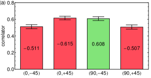
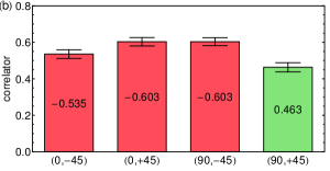
Figure 3: Measured correlators $\left\langle\sigma_{a}\sigma_{b}\right\rangle$ for the run started on Apr. 15, 2016 for the atom-atom state $\left|\Psi^{-}\right\rangle$ (a) and $\left|\Psi^{+}\right\rangle$ (b). Displayed errors are equal to one standard deviation.

Explicit data for the above run, for the first violation in 2015, as well as of further runs are documented in the Supplemental Material sup Sec. VI. Especially, we want to point at the run started on June 14, 2016. The start of it was made public via the Twitter account @munichbellexp and simultaneously at a conference Vae . The results of each of the events, coming in at a rate of about $1/\mathrm{min}$, were directly communicated to a central server http://bellexp.quantum.physik.uni-muenchen.de, which made all the data available together with the momentary evaluation. In this public Bell test, due to the lower rate of trapping single atoms the $2\times 5000$ events were collected during a time of $10$ days, resulting in $S=2.134\pm 0.048$ ($\left|\Psi^{-}\right\rangle$) and $S=2.057\pm 0.048$ ($\left|\Psi^{+}\right\rangle$). The violations of $2.8$ and $1.2$ standard deviations result in P-values for the combined data of $P_{m}=0.0267$ and $P_{g}=2.82\cdot 10^{-3}$. It should be noted, that with the modest event rate the effect of counting statistics on the momentary value of the S-parameter became clearly visible to a wide audience. The complete data are available for download from the server.

Finally, we consider a further frequently mentioned loophole - the free-will (or freedom of choice) loophole Bell et al. (1985) targeting the independence of choice of the analysis directions from the hidden variables and vice versa Larsson (2014). Contrary to experiments with photon pairs Giustina et al. (2015); Shalm et al. (2015), event-ready tests using entanglement swapping do not have a typical moment where the LHVs would have been defined Branciard et al. (2010). If we assume that the LHVs are defined at the time of the BSM, in our experiment taking place $10.7\,\mu s$ before the choice of the local analysis directions, they are clearly not influenced by the latter. Yet, contrary, the random settings are determined within the light cone of the BSM and independence has to be assumed here. This was accounted for in Hensen et al. (2015); Giustina et al. (2015); Shalm et al. (2015) where generation of the random numbers is considered being outside of the light cone of the entanglement generation (allowing to exclude influences within one trial of the experiment up to a few nanoseconds for the photon experiments Giustina et al. (2015); Shalm et al. (2015) or $690\,\mathrm{ns}$ for the experiment using NV-centers Hensen et al. (2015)).

However, in the analysis of all experiments (including the present one) there is still the implicit assumption that the dependence of the random numbers generated for the $n$-th observation event on processes or events of any kind in their backward light cone is strongly limited (e.g., dependence on previous settings and outcomes of the experiment). Effectively, while one allows memory and by this dependence on the history for the LHV model determining the measurement outcomes, one does not allow memory for the (quantum) systems observed in the QRNGs to determine the settings. To avoid such assumptions - and the corresponding loopholes - and to warrant true independence of the random settings also in view of memory attributed to all quantum systems one should produce random numbers outside the light cones of all other events of the Bell test. Spacelike separated extraterrestrial sources of randomness are required and have to be developed to ensure this Gallicchio et al. (2014); *Handsteiner2017.

In this Letter we described a highly reliable event-ready Bell test, showing in several attempts a clear violation of a Bell inequality. With violations of more than $6$ standard deviations obtained in a run with $10000$ events the probability that this actual result could be described by local hidden variables is at most $P_{m}=2.57\cdot 10^{-9}$. Taking all data accumulated during a time period of $7$ months with over $55000$ events (without any postselection) decreases this value to $P_{m}=1.02\cdot 10^{-16}$. On the fundamental side, further reducing the number of assumptions on the independence of the randomness generation makes the development of methods for employing extraterrestrial sources highly desirable. From the point of view of applications, where the requirements for the random setting choice are different, our essentially loophole-free Bell test forms a promising platform for device-independent secure communication. The methods and results achieved here pave the way for new developments of quantum information and for future quantum repeater networks.

Supplemental material

I Experimental Details

I.1 Synchronization and control of the experiment

The experiment consists of two independent atom traps connected by a $700\,\mathrm{m}$ long fiber link for photons emitted by trapped atoms as well as for synchronization and communication between the two setups. All communication between the two sides is done optically at telecom wavelength (Fig. S1, fibers 2-6). Depending on the specific requirements the signals are transmitted via analog (a), digital (d) or network (n) electro-optical converters. Each trap is controlled locally by a PC and a custom-built pattern generator that is used as a control unit (CU). The PC next to trap 1 acts as master. It is capable of controlling the remote PC in lab 2 by sending commands via an optical network connection (fiber 5). It also continuously analyzes the photon counts collected from both traps via the 4 avalanche photo diodes (APDs) of the BSM arrangement. The CUs operate at a clock speed of $50\,\mathrm{MHz}$ and thus a resolution of $20\,\mathrm{ns}$ with a timing jitter of $<40\,\mathrm{ps}$. They are capable of switching lasers and logic signals in a programmable way and also respond to external signals. All timing-critical components are synchronized to a common $100\,\mathrm{MHz}$ clock located in lab 2 whose signal is distributed via fiber 2. Synchronization of the CUs is monitored by a synchronization unit in lab 1 with the help of an additional signal transmitted via fiber 4 guaranteeing altogether a low relative jitter of less than $150\,\mathrm{ps}$ rms betwen the two labs. A time-to-digital converter (TDC) with a time resolution of $80\,\mathrm{ps}$, connected to the master PC, records all necessary time stamps, e.g., all photons counts and time markers generated by CUs indicating the different sequences in the experiment.

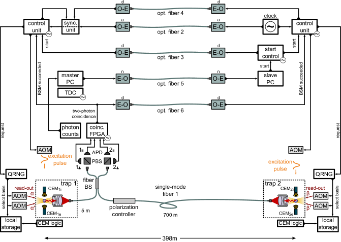
Figure S1: Synchronization and control of the experiment. Some signals are omitted for simplicity. Devices marked with a \textasciitilde{}⃝ symbol are synchronized to the common $100\,\mathrm{MHz}$ clock. AOM: acousto-optic modulator, APD: avalanche photo diode, BS: beam splitter, CEM: channel electron multiplier, EO/OE: electro-optic/opto-electric converters for analog (a), digital (d) or network (n) signals, FPGA: field programmable gate array, PBS: polarizing beam-splitter, QRNG: quantum random number generator.

I.2 Experimental sequence

Loading of the atom traps is controlled by the PCs. Depending on the level of photon counts integrated within $40\,\mathrm{ms}$, it is distinguished whether atoms are present in the two traps and loading operations are initialized accordingly. Loading of both atom traps takes typically about $2-3\,\mathrm{s}$.

After both traps are loaded the master PC initiates switching of the two CUs to the excitation sequence (Fig. S2). The required signal is generated by the start control unit (SCU) in lab 2 and communicated to lab 1 via fiber 3 (Fig. S1). The excitation sequence consists of preparation of the $5^{2}S_{1/2},F=1,m_{F}=0$ by optical pumping followed by excitation to the $5^{2}P{}_{3/2},F^{\prime}=0,m_{F^{\prime}}=0$ state. After each excitation there is a waiting time of $7.3\,\mathrm{\mu s}$ needed to transmit the photons from trap 2 to the BSM setup in lab 1 and to transmit a potential two-photon detection signal back to lab 2. This procedure is performed in repeated bursts that are timed such that the emitted photons of both trap setups have a temporal overlap close to unity at the BSM arrangement. A successful BSM is registered by one of four characteristic two-photon detection events ($1_{\perp}2_{\parallel}$ or $1_{\parallel}2_{\perp}$ for $\left|\Psi^{-}\right\rangle$ and $1_{\perp}1_{\parallel}$ or $2_{\perp}2_{\parallel}$ for $\left|\Psi^{+}\right\rangle$) in a time-window of $120\,\mathrm{ns}$ Hofmann et al. (2012). If one of those two-photon detections has occurred, signals are sent to both CUs to switch to the state measurement. Otherwise after $40$ preparation-excitation cycles the atoms are recooled for $350\,\mathrm{\mu s}$ and the sequence is restarted giving an average rate of excitation attempts is $5.2\times 10^{4}\,\mathrm{s^{-1}}$. If the master PC registers loss of one of the atoms the corresponding trap is reloaded.

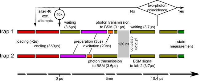
Figure S2: Experimental sequence.

I.3 Detailed timing scheme of the atomic state measurement

Fig. S3 shows the measured timings of all relevant processes of the atomic state measurement after a two-photon coincidence. The state-measurements have to be space-like separated which requires fast measurements with precisely known timings.

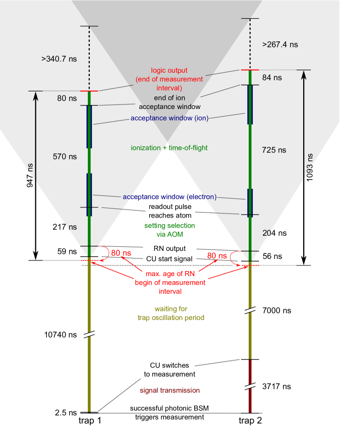
Figure S3: Detailed timing scheme of the experimental sequence after successful BSM.

The common start signal for the state-measurement is generated in lab 1 by a FPGA registering a two-photon coincidence in the BSM arrangement. This signal is distributed to both control units (CUs) locally via a $50\,\mathrm{cm}$ coaxial cable and via the $700\,\mathrm{m}$ long optical link for the distant location. The propagation time is measured by the delay of a signal transmitted to the remote location and back. This yields signal transmission times of $2.5\pm 0.2\,\mathrm{ns}$ and $3717\pm 7\,\mathrm{ns}$, respectively. Additional waiting times on both sides are necessary to minimize dephasing of the atomic state which are chosen such that the state measurement is performed after a full transverse oscillation period of the atom in the respective trap. The CU in lab 1 waits $10.74\,\mathrm{\mu s}$ and in lab 2 waits $7.00\,\mathrm{\mu s}$, respectively, before a measurement start signal is issued. With this the measurements in the two traps start almost simultaneously (trap 2 starts $28.5\,\mathrm{ns}$ earlier).

First, a random bit is requested determining the measurement direction and, in our setup, determining which of the two acousto-optic modulators (AOMs) is activated to switch readout laser beam with the respective polarization. The switching times of the AOMs, given by the propagation of the acoustic wave in the crystal, together with propagation delays in cables, electronic components, and the optical path of the readout pulse to the position of the atom are measured with fast photo diodes placed in an equivalent distance to the atom traps. The delays between the output of a random bit and the beginning of the ionization process are $217\pm 4\,\mathrm{ns}$ and $204\pm 4\,\mathrm{ns}$. The time of flight of electrons towards the channel electron multipliers (CEMs) was calculated to be $3\,\mathrm{ns}$. Using this, the ionization time and time of flight of the ions to the CEMs are extracted from the arrival time histogram of electrons and ions. With these times at the beginning of measurement run we define two fixed time-windows for accepting electron and ion detection events chosen to optimize the signal to noise ratio for better fidelity. In the presented measurement runs the lengths of these windows were $240\,\mathrm{ns}$ ($160\,\mathrm{ns}$) for electrons and $240\,\mathrm{ns}$ ($220\,\mathrm{ns}$) for ions for trap 1 (trap 2). The maximal time for ionization and flight given by the end of the ion acceptance window is $570\pm 3\,\mathrm{ns}$ and $725\pm 3\,\mathrm{ns}$ for the two traps, respectively (the uncertainty results from the rising edge in the electron arrival time histogram at the beginning of the process). These are different for two traps as the acceleration voltages between the CEMs differ to avoid high-voltage breakdowns in trap 2.

The measurement is considered finished when the detection clicks of the CEMs are transformed to a logic pulse in electronics outside the vacuum chamber which happens $80\,\mathrm{ns}$ and $84\,\mathrm{ns}$ after the detection. Together with the time of the RN generation/correlation of $80\,\mathrm{ns}$ this results in the overall measurement time of $947\pm 1\,\mathrm{ns}$ and $1093\pm 1\,\mathrm{ns}$, respectively. Note that this time is known with a high precision as it is based on signals of the CU (starting signal of the measurement and the end of the ion acceptance window). The stated uncertainty results mostly from the additional signal processing units (like signal converters, etc.).

I.4 Criteria of space-like separation

The distances between the laboratories and in particular between the QRNGs and atom traps were determined by combining measurements within the buildings with maps and building outlines provided by the Bavarian land surveying office ver . The positions of the atom trap and the QRNG in each lab were determined with respect to a reference position at the outer corner of the building in three dimensions with an accuracy of better than $10\,\mathrm{cm}$. The accuracy of this measurement guarantees that for each point the real position is within a volume of $0.5\,\mathrm{m}$ radius around the measured position. The coordinates of the reference points, the orientations of the buildings and respective altitudes were extracted from the provided data ver . By these means the measured distances between the QRNGs and atom traps are $398.0\,\mathrm{m}$ (QRNG 2 $\leftrightarrow$ trap 1) and $402.7\,\mathrm{m}$ (QRNG 1 $\leftrightarrow$ trap 2). Assuming maximal errors favoring the shortest distance we arrive at minimal time for a luminal signal to reach the other side of $(398.0\,\mathrm{m}-2\cdot 0.5\,\mathrm{m})/c=1324.2\,\mathrm{ns}$ and $(402.7\,\mathrm{m}-2\cdot 0.5\,\mathrm{m})/c=1339.9\,\mathrm{ns}$, respectively.

Taking the values from section I.3, the maximal measurement times are $947+1\,\mathrm{ns}=948\,\mathrm{ns}$ and $1093+1\,\mathrm{ns}=1094\,\mathrm{ns}$. The uncertainty of the signal transmission time (Sec. I.3) leads to an uncertainty in the measurement start time for trap 2 of $\pm 7\,\mathrm{ns}$. Since the atomic state measurement in trap 2 starts $28.5\,\mathrm{ns}$ earlier, space-like separation is therefore guaranteed with remaining margins of $1324.2\,\mathrm{ns}-28.5\,\mathrm{ns}-7\,\mathrm{ns}-948\,\mathrm{ns}=340.7\,\mathrm{ns}$ and $1339.9\,\mathrm{ns}+28.5\,\mathrm{ns}-7\,\mathrm{ns}-1094\,\mathrm{ns}=267.4\,\mathrm{ns}$ (Fig. S3). By further delaying the measurement at trap 1 the margin could in principle be made symmetric at $304.0\,\mathrm{ns}$.

I.5 Data recording

For evaluation of the experiment we use two independent ways for data recording. First, for every successful BSM event, the resulting Bell state, the requested random bit and the measurement outcomes (CEM signals) are recorded locally on both sides (“local storage” in Fig. S1). This enables an evaluation of correlations and of Bell’s inequality. Second, the TDC records time stamps of all photons registered in the BSM arrangement, as well as of the requested random bits and CEM detection clicks from both sides. Additional signals indicating the position in the experimental sequence are stored in this data stream enabling a complete analysis of the experiment.

II Generation of Random Settings

For performing a test of Bell’s inequality free of the locality loophole the choices of the measurement directions, in the ideal case, are perfectly unpredictable. In our experiment these choices are derived from the outputs of quantum random number generators (QRNGs) which are unpredictable according to the physical model of the QRNGs. Technical imperfections can lead to a residual predictability of the output bit sequences which has to be taken into account in the analysis of the experimental results (Sec. III). In particular to derive the P-values one requires the maximal deviation $\tau$ from perfect unpredictability, which is defined such that for all output bits $q_{i}$: $\frac{1}{2}-\tau\text{$\leq$}Pr(q_{i}=0)\leq\frac{1}{2}+\tau$. In the following we describe the function of the employed QRNGs and estimate their predictability from a model. Furthermore we perform evaluation of bias, serial correlations and general statistical tests. Although statistical testing can never certify real randomness, it is the method of choice for testing the hypothesis of the bit sequence being random. Moreover, it still gives some information about the quality of randomness of the bits obtained from the QRNGs and allows identifying potential artifacts.

II.1 Random number generators

The method used for the random number generator (QRNG) Fürst et al. (2010) is based on counting the number of photons emerging from a light emitting diode (LED) source, passing an attenuator and detected by a photo-multiplier tube (PMT). The analog pulses at the output of the PMT are digitized by a comparator and counted within time bins of $20\,\mathrm{ns}$. The parity of the registered photon number finally constitutes the random bit.

The physical model employs the fact that according to photodetection theory Glauber (2007); Loudon (1997) the detection events from a broadband light source of constant power are fully uncorrelated on the timescale of the counting interval. In particular, each photon is assumed to be registered by the detector at an unpredictable time which is independent of any previous events in the backward light-cone as well as of the LHVs in the experiment. This leads to a Poissonian distribution of the detected photon numbers at the PMT. In our implementation the extendable dead time of the detector, i.e. its inability to register pulses arriving in a short succession which are interpreted as one long pulse, modifies this distribution Fürst et al. (2010), Fig.2. This is analogous to a real-time hardware processing additionally allowing to avoid bias of the output bits without the need for any further post-processing Fürst et al. (2010). Here we also assume that the detector itself can not be influenced within the LHV model.

In the experiment the QRNGs are operated at a speed of $50\,\mathrm{Mbps}$ and provide the last generated random bit on request within $8\,\mathrm{ns}$. Including all hardware latencies, the maximal “age” of this bit is $60\,\mathrm{ns}$ since the emission of the detected, contributing photon(s). The generators exhibit a modest next neighbor correlation of typically $<1.5\cdot 10^{-5}$ while all evaluated correlations with higher lag were found to be compatible with zero (see below). We thus include $20\,\mathrm{ns}$ for generation of the previous random bit and consider the output to be at most $80\,\mathrm{ns}$ “old”. All bits generated during an experimental run were continuously recorded for analysis purposes (organized in files of $1\,\mathrm{Gb}$) . The QRNGs incorporate continuous stabilization and monitoring of temperature and count rate to allow for long-term operation.

II.2 Estimation of predictability

While the emission and detection of photons are intrinsically random fundamental processes at the current state of knowledge, there are further technical parameters which may affect the output bit. Depending on the model, such parameters may be accessible when the outputs $A$, $B$ are generated by the observers and thus increase the predictability. The crucial parameters of the generators used are the average photon count rate, the threshold level of the comparator digitizing the PMT output pulses (influencing the extendable dead time Fürst et al. (2010)) and the temperature of the QRNG devices.

Photon count rate

For a given threshold of the PMT pulse comparator, the bias of the QRNG is a function of the photon count rate. Thus knowledge of the count rate allows a certain predictability. Before each measurement run the QRNGs are operated for a longer period to determine the count rate for minimal bias. During the measurement run the count rate is stabilized at this value by a feedback loop controlling the LED current. Once fixed, the count rate shows only expected statistical fluctuations. While this already shows the high stability of the involved components, we have additionally characterized the sensitivity of the bias to the LED current leading to effects much lower then the error made when determining the optimal count rate for minimal bias. This leads to a residual bias of typically between $10^{-6}$ and $10^{-5}$ (see Tab. S1).

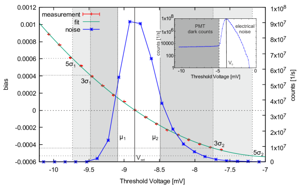
Figure S4: Measured bias (red crosses, approximated by second order polynomial green fit curve) as a function of the comparator threshold voltage level for the QRNG operated at typical LED current. The inset shows the distribution of registered counts as a function of the threshold voltage for LED switched off revealing the electrical noise and dark counts of the PMT. The blue stars in the main graph show the measurement from the inset on a linear scale and additionally centered around the set value of the threshold voltage $V_{set}$ (thus being equivalent to an integrated histogram of effective fluctuations of the set value). We approximate the rising and falling slope of the electrical noise part by error functions of the form $a\cdot(\mathrm{erf}(\frac{\mu-v_{thr}}{\sqrt{2}\sigma})+1)$ from both sides yielding the $3\sigma$ and $5\sigma$ intervals of amplitude fluctuations. This allows us to determine the maximal predictability for the corresponding confidence levels.

Threshold level of the comparator

Any fluctuations of the threshold level, or complementary any noise on the signal from the PMT will lead to a time-dependent bias and predictability. We thus analyze the bias for different threshold levels at a constant LED current. The result is shown in Fig. S4(red crosses). In a second measurement we have determined the distribution of registered counts with LED being switched off. Here we can observe two regions - one dominated by the dark counts of the PMT ($<-5\,\mathrm{mV}$) and one dominated by the electrical noise (Fig. S4, inset). For further analysis we assume that the measured data is an integrated histogram of the the noise amplitude distribution. We thus approximate the rising and the falling slopes of the electrical noise part (S4, blue stars) which is centered around the threshold set voltage by error functions obtaining the mean value $\mu_{1}=-9.09\,\mathrm{mV}$ and standard deviation $\sigma_{1}=0.13\,\mathrm{mV}$ on the rising side and $\mu_{2}=-8.48\,\mathrm{mV}$ and standard deviation $\sigma_{2}=0.25\,\mathrm{mV}$ on the falling side. Since the electrical noise adds to the real PMT pulses, it can be considered equivalent to noise of the comparator threshold level. Thus the influence of this noise on the predictability (bias) can be directly derived from these numbers. For a “paranoid” model which grants the LHV-controlled observers full knowledge about the noise of the QRNG in the distant lab we can now consider either the average over the time-dependent predictability or merely the maximal predictability (within a $5\sigma$ confidence interval). In the latter, most paranoid, case we arrive at a maximal additional predictability of $\tau=6.12\cdot 10^{-4}$.

Temperature of the QRNG device

The temperature of the critical part of the QRNG including LED, PMT and the comparator is actively stabilized to better than $\pm 0.15\,\mathrm{{}^{\circ}C}$. Still, the residual fluctuations, which may be accessible, can influence the critical threshold level of the comparator. Here the specified temperature coefficients of the comparator offset voltage and of the DAC providing the threshold level are both $10^{-5}\,\mathrm{V/^{\circ}C}$. This gives together with the bias dependence from above (S4) an additional predictability of $\tau=6.7\cdot 10^{-6}$ (in the case the effects add up).

Resulting predictabilities

Let us distinguish two models:

• a (reasonable) model where the information on the internal parameters of the QRNG are inaccessible except for temperature and the count rate (which are both stabilized and monitored with information being available externally). The resulting deviations of the generated bit sequence from an ideal random one determine the bias of the sequence. The maximal observed bias over all measurements (Tab. S1) is $8.74\cdot 10^{-6}$, compatible with the expectation. Taking this value and additionally adding a $2\sigma$ margin to it we can conservatively estimate a deviation from perfect unpredictability of $\tau_{1}=1.04\cdot 10^{-5}$.

• a (very paranoid) model where also the full information on the internal noise at the comparator is known and can be used when determining the measurement result according to such LHV models. This allows for an additional predictability which might not be visible in any typical statistical test. Note that exploiting this information for the distant lab requires extrapolation of the noise behavior for $1.3\,\mathrm{\mu s}$ into the future. With this ability granted, we sum over all above effects (error in the setting of photon count rate, noise on the threshold level, temperature dependence) arriving at a $\tau_{2}<6.3\cdot 10^{-4}$. We take this value for calculation of all P-values allowing us to exclude even such models.

We note that the predictabilites, even in the paranoid models, can be significantly reduced by performing an XOR operation on several successive output bits thereby combining them into one bit. This operation can be efficiently performed in hardware. In our experiment the time budget allows for combining at least $13$ bits, while $\tau$ would be $<10^{-6}$ already for a combination depth of $2$ bit.

II.3 Bias

We have evaluated the bias $B=\frac{n_{0}}{n}-\frac{1}{2}$ ($n_{0}$ being the number of ones in a sample of $n$ bits) of the generated bit sequences. Figure S5 shows an example of the observed bias as a function of time for one of the measurement runs. The bin size is chosen large enough for the statistical noise to be smaller than the observed value, which still allows observing possible drifts on a long time scale. Table S1 gives an overview of the data and the maximal observed bias for different measurement runs.

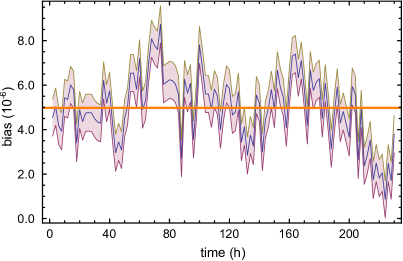
Figure S5: Time evolution of the bias in lab 1 for the measurement run on June 14, 2016. Each bin contains $360\,\mathrm{Gb}$ of data, corresponding to $2\,\mathrm{h}$ of measurement time. The shaded area represents a $\pm\sigma$ interval. The orange line shows the average value.

run	#bits	$\max(\left|B\right|)_{a}$	$\max(\left|B\right|)_{b}$	$\sigma$
Nov. 27, 2015	$2\times 10.6\,\mathrm{Tb}$	$2.66\cdot 10^{-6}$	$4.76\cdot 10^{-6}$	$8.33\cdot 10^{-7}$
Apr. 04, 2016	$2\times 8.0\,\mathrm{Tb}$	$4.04\cdot 10^{-6}$	$2.99\cdot 10^{-6}$	$8.33\cdot 10^{-7}$
Apr. 15, 2016	$2\times 16.0\,\mathrm{Tb}$	$4.33\cdot 10^{-6}$	$3.22\cdot 10^{-6}$	$8.33\cdot 10^{-7}$
June 14, 2016	$2\times 41.6\,\mathrm{Tb}$	$8.74\cdot 10^{-6}$	$7.15\cdot 10^{-6}$	$8.33\cdot 10^{-7}$

Table S1: Bias for various measurement runs. $\sigma$ corresponds to the standard deviation in a $360\,\mathrm{Gb}$ bin.

II.4 Correlations

For each measurement and both random number generators we analyzed the data of every file for serial correlations (or autocorrelation) according to

$$SCC_{l}=\frac{\sum_{k=1}^{n-l}(q_{k}-\frac{1}{2})(q_{k+l}-\frac{1}{2})}{\sum_{k=1}^{n}(q_{k}-\frac{1}{2})^{2}}$$

where $q_{k}\in\{0,1\}$ are the bits and $l$ is the lag (we evaluated correlations up to a lag of $56$). This formula is not corrected for bias which in our case would lead only to negligible corrections. All correlations with lag $l>1$ were found to be consistent with zero. Tab. S2 exemplarily shows the correlations for one of the measurement runs. We also evaluated the time evolution of $SCC_{1}$, only a small variation could be observed within $\sim 230\,\mathrm{h}$ of measurement time, see Fig. S6.

$l$	$SCC_{l}$	$l$	$SCC_{l}$	$l$	$SCC_{l}$	$l$	$SCC_{l}$	$l$	$SCC_{l}$	$l$	$SCC_{l}$
1	$\phantom{-}1.32\cdot 10^{-5}$	11	$-2.13\cdot 10^{-7}$	21	$-2.46\cdot 10^{-7}$	31	$-2.97\cdot 10^{-7}$	41	$-3.33\cdot 10^{-7}$	51	$\phantom{-}1.57\cdot 10^{-7}$
2	$\phantom{-}1.47\cdot 10^{-7}$	12	$-2.40\cdot 10^{-7}$	22	$-1.60\cdot 10^{-7}$	32	$\phantom{-}8.58\cdot 10^{-8}$	42	$\phantom{-}2.74\cdot 10^{-7}$	52	$-3.43\cdot 10^{-7}$
3	$-9.79\cdot 10^{-8}$	13	$-1.52\cdot 10^{-7}$	23	$\phantom{-}1.94\cdot 10^{-7}$	33	$\phantom{-}8.53\cdot 10^{-8}$	43	$\phantom{-}5.56\cdot 10^{-10}$	53	$-5.15\cdot 10^{-8}$
4	$\phantom{-}3.41\cdot 10^{-8}$	14	$-1.75\cdot 10^{-8}$	24	$\phantom{-}4.48\cdot 10^{-8}$	34	$\phantom{-}2.52\cdot 10^{-8}$	44	$\phantom{-}1.04\cdot 10^{-7}$	54	$\phantom{-}1.49\cdot 10^{-7}$
5	$\phantom{-}5.87\cdot 10^{-9}$	15	$-3.31\cdot 10^{-8}$	25	$\phantom{-}1.42\cdot 10^{-7}$	35	$-1.22\cdot 10^{-7}$	45	$\phantom{-}2.13\cdot 10^{-8}$	55	$\phantom{-}2.20\cdot 10^{-7}$
6	$-8.19\cdot 10^{-8}$	16	$-1.60\cdot 10^{-8}$	26	$-1.22\cdot 10^{-7}$	36	$\phantom{-}6.94\cdot 10^{-8}$	46	$-2.45\cdot 10^{-7}$	56	$\phantom{-}9.64\cdot 10^{-9}$
7	$-4.74\cdot 10^{-8}$	17	$\phantom{-}5.42\cdot 10^{-8}$	27	$-1.79\cdot 10^{-7}$	37	$\phantom{-}1.19\cdot 10^{-7}$	47	$-2.83\cdot 10^{-8}$
8	$\phantom{-}1.38\cdot 10^{-7}$	18	$\phantom{-}6.01\cdot 10^{-8}$	28	$-3.26\cdot 10^{-7}$	38	$-1.99\cdot 10^{-8}$	48	$-2.43\cdot 10^{-7}$
9	$\phantom{-}1.62\cdot 10^{-7}$	19	$\phantom{-}1.49\cdot 10^{-7}$	29	$-4.92\cdot 10^{-8}$	39	$\phantom{-}9.53\cdot 10^{-8}$	49	$-2.90\cdot 10^{-7}$
10	$\phantom{-}2.19\cdot 10^{-7}$	20	$-7.91\cdot 10^{-8}$	30	$\phantom{-}1.56\cdot 10^{-8}$	40	$-2.39\cdot 10^{-7}$	50	$\phantom{-}1.65\cdot 10^{-8}$

Table S2: Averaged correlations in lab 1 for the measurement run on June 14, 2016. The statistical errors of all correlations in this data set are $\sigma=1.55\cdot 10^{-7}$ (one standard deviation).

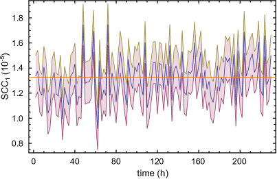
Figure S6: Time evolution of $SCC_{1}$ in lab 1 for the measurement run on June 14, 2016. Each bin contains $360\,\mathrm{Gb}$ of data, corresponding to $2\,\mathrm{h}$ of measurement time. The shaded area represents a $\pm\sigma$ interval. The orange line shows the average value of $1.32\cdot 10^{-5}$.

II.5 Statistical tests

We tested the output bitsequences of the QRNGs using the statistical test suite “TestU01 Alphabit battery” L’Ecuyer and Simard (2007). We applied these tests to all bits collected during the measurement runs on Apr. 15, 2016 and June 14, 2016, which are $115420$ files ($115\,\mathrm{Tb}$ in total). For each data file, all statistical tests were applied and the resulting P-values for the null hypothesis of randomness (iid bits with $Pr(q_{i}=1)=Pr(q_{i}=0)=\frac{1}{2}$) were calculated. In the ideal case the P-values are expected to be uniformly distributed. This was observed for all of our data and all tests in the battery except for the test row smultin_MultinomialBitsOver (test on uniformity of appearance of bit chains of certain length, evaluated using overlapping serial approach), see Table S3. There the P-value distribution is shifted towards $0$. To understand this behavior we applied a related test smultin_MultinomialBits (the same as above but evaluated using non-overlapping serial approach) which can be easier modeled using a noncentral $\chi^{2}$-distribution. Fig. S7 shows that our model which includes only the known bias and next-neighbor correlation fits the data well. Thus the applied set of tests did not reveal any effects in the data which are stronger than the next-neighbor correlation. Note that these subtle effects are only visible due to the large amount of data available. Alltogether our findings support the thesis that the bits are in fact random and well-suited for our application.

	April 15, 2016		June 14, 2016
Test	P-value lab 1	P-value lab 2	P-value lab 1	P-value lab 2
smultin_MultinomialBitsOver with L = 2	$3.83\cdot 10^{-20}$	$1.66\cdot 10^{-5}$	$6.06\cdot 10^{-123}$	$4.11\cdot 10^{-44}$
smultin_MultinomialBitsOver with L = 4	$7.65\cdot 10^{-9}$	$1.86\cdot 10^{-4}$	$2.95\cdot 10^{-58}$	$6.92\cdot 10^{-26}$
smultin_MultinomialBitsOver with L = 8	$0.298$	$0.542$	$8.14\cdot 10^{-3}$	$0.061$
smultin_MultinomialBitsOver with L = 16	$0.347$	$0.086$	$0.842$	$0.815$
sstring_HammingIndep with L = 16	$0.663$	$0.824$	$0.065$	$0.822$
sstring_HammingIndep with L = 32	$0.499$	$0.838$	$0.997$	$0.043$
sstring_HammingCorr with L = 32	$0.275$	$0.674$	$0.435$	$0.008$
swalk_RandomWalk1 with L = 64 (Statistic H)	$0.413$	$0.942$	$0.045$	$0.208$
swalk_RandomWalk1 with L = 64 (Statistic M)	$0.166$	$0.646$	$0.376$	$0.892$
swalk_RandomWalk1 with L = 64 (Statistic J)	$0.496$	$0.684$	$0.506$	$0.899$
swalk_RandomWalk1 with L = 64 (Statistic R)	$0.092$	$0.287$	$0.801$	$0.544$
swalk_RandomWalk1 with L = 64 (Statistic C)	$0.676$	$0.594$	$0.712$	$0.240$
swalk_RandomWalk1 with L = 320 (Statistic H)	$0.963$	$0.761$	$0.334$	$0.663$
swalk_RandomWalk1 with L = 320 (Statistic M)	$0.534$	$0.138$	$0.575$	$0.241$
swalk_RandomWalk1 with L = 320 (Statistic J)	$0.487$	$0.196$	$0.253$	$0.881$
swalk_RandomWalk1 with L = 320 (Statistic R)	$0.032$	$0.471$	$0.291$	$0.715$
swalk_RandomWalk1 with L = 320 (Statistic C)	$0.941$	$0.608$	$0.930$	$0.173$

Table S3: Results of the TestU01 Alphabit test battery for the measurement runs on April 15, 2016 and June 14, 2016. On each side the tests were applied to $16072$ and $41638$ files of $1\,\mathrm{Gb}$ for the two runs, respectively. The resulting distributions of P-values for each test were checked for uniformity with a $\chi^{2}$-test, whose P-values are shown here.

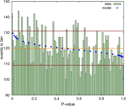
Figure S7: Histogram of P-values in the serial test smultin_MultinomialBits with block length of $4$ bits applied to the data from lab 1 in the measurement run on April 15, 2016. The orange line corresponds to the average value, the red lines to the $\pm\sigma$ interval of the bins. The blue dots result from the model based on bias and next-neighbor correlations of this data set.

III Testing LHV Theories

The main goal of Bell experiments is to rule out all local-hidden-variable (LHV) theories by measuring a violation of Bell’s inequality. Since real experiments can only generate a finite amount of data, even an experiment governed by LHVs may still exhibit a violation of Bell’s inequality by chance. To account for this, one estimates the probability that a specific violation or a more extreme one can be produced by an experiment governed by LHVs. If this probability is small for an experimental outcome it is fair to reject the hypothesis of LHVs with a certain confidence. This procedure is called a null hypothesis test and the respective probability is called a P-value. For a null hypothesis test of the validity of LHV theories we have to find the probability distribution for the $S$-values under the assumption of LHVs. With this probability distribution we can calculate the P-value for any measured value of $S$.

When performing such an analysis, one needs to be careful not to introduce additional assumptions into the model to be tested. The standard way of the evaluation of experimental data would be to assume Gaussian distribution of measurement results. Then the P-value can be easily calculated for the measured value of $S$ and its standard deviation. However, this requires the assumption that the experimental tries can be considered independent and identically distributed (iid) which is not necessarily valid. First, the experimental parameters may vary over the course of the experiment. Second, from the fundamental point of view, the knowledge of the history of previous settings and outcomes might allow for a LHV model violating Bell’s inequality (memory loophole). Depending on the formulation of the inequality this is indeed possible Barrett et al. (2002), although the violation approaches zero with increasing number of tries $N$. In any case an analysis procedure which does not require the assumption of iid is needed. Ways to achieve this include modeling of the underlying stochastic process as a martingale Gill (2003) or its formulation as a game Brunner et al. (2014); Elkouss and Wehner (2016), as well as prediction-based-ratio (PBR) approach Zhang et al. (2013).

III.1 Defining the null hypothesis

The first step is to formulate the null hypothesis in a way that we can use to calculate bounds on the P-value. For this we use the CHSH inequality as a mathematical formulation of the hypothesis and define it for our experiment.

Our Bell experiment employs two observers in lab 1 and lab 2. On receiving the heralding signal each side of the experiment gets an input for the setting selection and produces a measurement outcome (in the following we call such a process “event”). We name the inputs for the $i$-th of $N$ events $a_{i}\in\left\{\alpha,\alpha^{\prime}\right\}$ for lab 1 and $b_{i}\in\left\{\beta,\beta^{\prime}\right\}$ for lab 2. Similarly we name the measurement outcomes for this event $x_{i}$ for lab 1 and $y_{i}$ for lab 2 with $x_{i},y_{i}\in\left\{-1,1\right\}$ (outcome $\left|\uparrow\right\rangle$ corresponding to $1$, outcome $\left|\downarrow\right\rangle$ to $-1$). Since our experiment employs an event-ready scheme we name the event-ready signal for this event $h_{i}$, where $h_{i}=1$ heralds the $\Psi^{+}$-state and $h_{i}=-1$ heralds the $\Psi^{-}$-state.

We define the functions $g^{\pm}(a,b)$ for events with the event-ready signal $h_{i}$ for $\Psi^{+}$ or $\Psi^{-}$ that take the values $1$ or $-1$:

$$g^{+}(a,b) =-1\;\;\;\forall\>(a,b)\neq(\alpha^{\prime},\beta^{\prime})$$ (S1)

$$g^{+}(a,b) =\phantom{-}1\;\;\;\phantom{\forall}\>(a,b)=(\alpha^{\prime},\beta^{\prime})$$

$$g^{-}(a,b) =-1\;\;\;\forall\>(a,b)\neq(\alpha^{\prime},\beta)$$

$$g^{-}(a,b) =\phantom{-}1\;\;\;\phantom{\forall}\>(a,b)=(\alpha^{\prime},\beta)$$

With these functions we can write the CHSH inequality for each state in the form:

$$S^{\pm}=\sum_{\begin{subarray}{c}a\in\left\{\alpha,\alpha^{\prime}\right\}\\ b\in\left\{\beta,\beta^{\prime}\right\}\end{subarray}}g^{\pm}(a,b)\frac{{}^{C}N_{a,b}^{\pm}-{}^{A}N_{a,b}^{\pm}}{{}^{C}N_{a,b}^{\pm}+{}^{A}N_{a,b}^{\pm}}\leq 2.$$ (S2)

Here ${}^{C}N_{a,b}^{\pm}=N_{a,b}^{\uparrow\uparrow}+N_{a,b}^{\downarrow\downarrow}$ is the number of correlated measurement outcomes ($x_{i}=y_{i}$) and ${}^{A}N_{a,b}^{\pm}=N_{a,b}^{\uparrow\downarrow}+N_{a,b}^{\downarrow\uparrow}$ is the number of anticorrelated measurement outcomes ($x_{i}\neq y_{i}$), for state $\Psi^{\pm}$ respectively.

For large $N$ and low bias of the input random bits we can approximate ${}^{C}N_{a,b}^{\pm}+{}^{A}N_{a,b}^{\pm}$ with $N^{\pm}/4$ and obtain

$$S^{\pm}=\frac{1}{N^{\pm}}\sum_{i=1}^{N^{\pm}}4\cdot g^{\pm}(a_{i},b_{i})x_{i}y_{i}\leq 2.$$ (S3)

This form of Bell’s inequality is not susceptible to systematic violations exploiting finite statistics shown in Barrett et al. (2002).

III.2 Martingales and concentration inequalities

In order to estimate the P-value one can employ concentration inequalities which provide bounds on deviations of stochastic processes from their expectation values. Here we will use the Mc Diarmid inequality McDiarmid (1989) in the following way similar to Zhang et al. (2013). First we define the sequences

$$f_{i} =4\cdot g^{\pm}(a_{i},b_{i})x_{i}y_{i}$$ (S4)

$$\Rightarrow -4\leq f_{i}\leq 4$$

and

$$Z_{i} =\frac{f_{i}-2}{8}$$ (S5)

$$\Rightarrow -\frac{3}{4}\leq Z_{i}\leq\frac{1}{4}.$$

We can now write equation (S3) as

$$S^{\pm}=\frac{1}{N^{\pm}}\sum_{i=1}^{N^{\pm}}f_{i}$$ (S6)

and

$$\frac{1}{N^{\pm}}\sum_{i=1}^{N^{\pm}}Z_{i}=\frac{S^{\pm}-2}{8}$$ (S7)

is a measure for the violation of Bell’s inequality. For any experiment governed by LHVs saturating Bell’s inequality, $Z_{i}$ is a martingale difference sequence and we can use the equation (6.1) from McDiarmid (1989)

$$Pr(\sum_{i=1}^{N^{\pm}}Z_{i}\geq tN^{\pm})\leq\left[\left[\frac{A}{A+t}\right]^{A+t}\left[\frac{\bar{A}}{\bar{A}-t}\right]^{\bar{A}-t}\right]^{N^{\pm}}$$ (S8)

with $t=\frac{S^{\pm}-2}{8}$, $A=\frac{3}{4}$, and $\bar{A}=\frac{1}{4}$ to bound the probability of a certain violation $\delta$ or a more extreme one under assumption of LHVs, thereby obtaining the P-value $P_{m}$:

$$P_{m}=Pr(S-2\geq\delta)\leq\left[\frac{1}{\left(1+\frac{\delta}{6}\right)^{\frac{3}{4}+\frac{\delta}{8}}\cdot\left(1-\frac{\delta}{2}\right)^{\frac{1}{4}-\frac{\delta}{8}}}\right]^{N}.$$ (S9)

This bound is also valid for all LHV models which do not saturate Bell’s inequality, in which case the process is a supermartingale.

The limit of the $S$-value achievable with LHVs increases if the random bits are not ideal (partially predictable). The deviations from perfect unpredictability $\tau_{a},\tau_{b}\in\left[-\frac{1}{2},\frac{1}{2}\right]$ on the two sides are defined $\forall i$ by

$$\frac{1}{2}-\tau_{a}\text{$\leq$}Pr(a_{i}=\alpha|H_{i}) \leq\frac{1}{2}+\tau_{a}$$

$$\frac{1}{2}-\tau_{b}\text{$\leq$}Pr(b_{i}=\beta|H_{i}) \leq\frac{1}{2}+\tau_{b}$$ (S10)

where $H_{i}$ is the common history of the experiment at the $i$-th event, i.e. the complete information available to the two observers which can be used for predicting the setting choice on the other side.

For simplicity we set $\tau=\max(\left|\tau_{a}\right|,\left|\tau_{b}\right|)$. We note that the predictability may depend on the history of the experiment $H$

To calculate the effect of the predictability on the $S$-parameter we consider the following. For example let us assume that for a certain attempt $i$ where the atomic state $\left|\Psi^{+}\right\rangle$ was prepared, the probabilities of the setting inputs are $Pr(a_{i}=\alpha)=\frac{1}{2}+\tau$ and $Pr(b_{i}=\beta)=\frac{1}{2}+\tau$. This means that in this situation the probability of $(\alpha,\beta)$ input is the highest and of the $(\alpha^{\prime},\beta^{\prime})$ input is the lowest. An LHV strategy (of the $16$ possible) which would maximize the expectation value of $S$ for this attempt would be to produce anticorrelations for all input combinations. Then one obtains for this expectation value

$$\sum_{\begin{subarray}{c}a\in\left\{\alpha,\alpha^{\prime}\right\}\\ b\in\left\{\beta,\beta^{\prime}\right\}\end{subarray}}4\cdot g^{+}(a,b)\cdot x_{i}y_{i}\cdot Pr(a_{i}=a)Pr(b_{i}=b)=\\ =4\Big{(}(-1)(-1)(\frac{1}{2}+\tau)^{2}+(-1)(-1)(\frac{1}{2}+\tau)(\frac{1}{2}-\tau)\\ +(-1)(-1)(\frac{1}{2}-\tau)(\frac{1}{2}+\tau)+(+1)(-1)(\frac{1}{2}-\tau)^{2}\Big{)}=\\ =4\left(2\tau+2(\frac{1}{4}-\tau^{2})\right)=2+8(\tau-\tau^{2}).$$

As is easy to verify, for any combination of input setting probabilities and each atomic state there exists an LHV strategy achieving this value. Thus, by optimally switching strategies event for event, one obtains the expectation value

$$S\leq 2+8(\tau-\tau^{2}).$$

We consequentially use $t=\frac{S^{\pm}-2}{8}-(\tau-\tau^{2})$ , $A=\frac{3}{4}+(\tau-\tau^{2})$, and $\bar{A}=\frac{1}{4}-(\tau-\tau^{2})$ in (S8) for calculation of P-values.

To calculate the P-value for the combined data of $\Psi^{+}$- and $\Psi^{-}$- states we use

$$S=\frac{1}{N}\sum_{i=1}^{N}4\cdot\left[\frac{1+h_{i}}{2}g^{+}(a_{i},b_{i})x_{i}y_{i}+\frac{1-h_{i}}{2}g^{-}(a_{i},b_{i})x_{i}y_{i}\right]\leq 2.$$ (S11)

III.3 Game formalism

An alternative approach is to formulate a CHSH experiment as a game Elkouss and Wehner (2016). Here, LHV are represented by two parties which have to generate correlations or anticorrelations based on random inputs, where only the local input is known to each party during a game round. Otherwise they may employ any strategy which also may be adapted during the course of the game and are allowed to communicate between the rounds. To win the game they need to produce the right correlations (three anticorrelations, one correlation, depending on the input) maximal number of times.

To describe this formally, we define the functions $w_{i}^{+}$ for $\Psi^{+}$-events and $w_{i}^{-}$ for $\Psi^{-}$-events:

$$w_{i}^{\pm}=\frac{\left|g^{\pm}(a_{i},b_{i})+x_{i}y_{i}\right|}{2}.$$ (S12)

If $w_{i}^{\pm}=1$ the game is won for this round. Thus the total number of rounds won for each state is $W^{\pm}=\sum_{i=1}^{N}\frac{1\pm h_{i}}{2}w_{i}^{\pm}$. For LHV theories the probability of winning a single round of a CHSH-game is Elkouss and Wehner (2016)

$$Pr(w_{i}^{\pm}=1)\leq\xi=3/4+(\tau-\tau^{2}).$$ (S13)

Note that, if $\tau$ depends on the history of the experiment (Eq. (S10)), the winning probability will also depend on this history. Now we can calculate the probability $Pr(W,N)$ of winning at least $W$ times in $N$ rounds:

$$P_{g}\leq Pr(W,N)=\sum_{j=W}^{N}\binom{N}{j}\xi^{j}(1-\xi)^{N-j}.$$ (S14)

With the number of wins $W^{\pm}$ and number of events $N^{\pm}$ for each atomic state we can calculate a P-value $P_{g}$ for each state individually. To calculate a combined P-value for the complete experiment we define the function for a win for $\Psi^{+}$ and $\Psi^{-}$ events

$$w_{i}=\frac{1+h_{i}}{2}\frac{\left|g^{+}(a_{i},b_{i})+x_{i}y_{i}\right|}{2}+\frac{1-h_{i}}{2}\frac{\left|g^{-}(a_{i},b_{i})+x_{i}y_{i}\right|}{2}.$$ (S15)

The total number of wins for $\Psi^{+}$ and $\Psi^{-}$ is $W=W^{+}+W^{-}$ and can be put in Eq. (S14).

IV Avoiding Expectation Bias

An important property of any scientific experiment should be impartiality. This implies that the assessment of the results has to be based on objective criteria only, devoid of any expectation on the outcome. If no special care is taken about this, results can easily become biased towards the expectation (see, e.g., Jeng (2006)). This can happen, e.g., by conscious or unconscious discarding of data which apparently do not fit the expected value. Publishing predominantly positive results can lead to a distorted picture in the literature, known as the “publication bias”. Vice versa, distorted values in the literature may influence new experiments.

The number of parameters in a complex experiment can be large making it difficult to define a complete set of objective criteria for a decision whether a certain experimental run is valid or not. However, one must not decide on its validity by looking at the result. This also prohibits discarding parts of the data where the result deviates from the expectation or stopping the run prematurely when the result appears acceptable. Doing so will lead to apparently “better” results (“P-value hacking”).

To account for this problem we defined a list of rules before a run is started (we admit that completely avoiding bias is extremely difficult and our measures might not be complete):

• The number of events to be accumulated is fixed beforehand.

• The acquisition procedure is fixed beforehand. This includes all acceptance time-windows (two-photon coincidence, CEM detections).

• The analysis procedure is fixed beforehand. This includes the calculation of $S$ and P-values.

• Exclusion of events during the experimental run is based only on the two following criteria:

  • laser stability: on each side all stabilized lasers are fed into a scanning Fabry-Perot resonator whose output is measured with a photodiode. The resulting spectrum is represented with an oscilloscope and monitored by a camera. This allows us to (manually) determine the time when a malfunction appeared and to exclude all events between this time and until the problem is fixed. Malfunctions of most lasers will yield no events (as no atoms will be loaded), however problems with the readout laser reduce the fidelity and such events have to be excluded.

  • CEMs: a high-voltage breakthrough in the detector system can lead to a shutdown. In this case all events are automatically excluded until the problem is fixed.

• The maintenance procedure is performed every 24 hours and is limited to:

  • check of the laser system (frequency stabilization and optical power at all relevant positions),

  • compensation of magnetic fields (for all $3$ axes with a precision of $0.5\,\mathrm{mG}$),

  • minimization of polarization rotation in the fibers of the beam splitter in the BSM arrangement including the $5\,\mathrm{m}$ fiber connecting trap 1 to the BSM. Together with the automatic polarization compensation procedure of the $700\,\mathrm{m}$ fiber from trap 2 this ensures that there is no polarization rotation between different inputs and outputs of the BS in the two-photon interference process.

V Public Measurement Run

On top of obtaining a conclusive violation of Bell’s inequality, an additional goal of our project was to perform an open scientific experiment. This includes defining the rules in advance to avoid expectation bias, as well as making all data available to the public during the whole course of the experiment. For this purpose we have set up a web server http://bellexp.quantum.physik.uni-muenchen.de. All incoming data and other relevant information is presented there in real-time. Important information concerning the measurement is logged and distributed via the Twitter account @munichbellexp.

The public run was started on June 14, 2016 with the goal to collect $5000$ events for each of the two prepared atomic states. The run took $10$ days including daily maintenance stops. While the obtained violation (Tab. S10) is weaker than in other runs, it is still significant. Note that the situation where a certain measurement run yields results below average is to be expected, the same way results that appear above the average can be obtained due to purely statistical effects.

VI Data Tables

Experimental data is available online at

http://bellexp.quantum.physik.uni-muenchen.de.

VI.1 Run on Nov. 27, 2015

Nov. 27, 2015, $\Psi^{+}$
$\alpha,\beta$	$\uparrow\uparrow$	$\uparrow\downarrow$	$\downarrow\uparrow$	$\downarrow\downarrow$	total	$\left\langle\sigma_{\alpha}\sigma_{\beta}\right\rangle$
0,-45	4	16	21	4	45	$-0.644\pm 0.114$
0,-45	4	12	13	4	33	$-0.515\pm 0.149$
90,-45	3	24	11	2	40	$-0.750\pm 0.105$
90,-45	10	4	8	10	32	$\phantom{-}0.250\pm 0.171$
$S$					150	$\phantom{-}\mathbf{2.160\pm 0.279}$
$P_{m}$						$0.7009$
$P_{g}$	117 wins					$0.2328$

Nov. 27, 2015, $\Psi^{-}$
$\alpha,\beta$	$\uparrow\uparrow$	$\uparrow\downarrow$	$\downarrow\uparrow$	$\downarrow\downarrow$	total	$\left\langle\sigma_{\alpha}\sigma_{\beta}\right\rangle$
0,-45	4	11	17	2	34	$-0.647\pm 0.131$
0,-45	4	16	13	3	36	$-0.611\pm 0.132$
90,-45	22	4	2	10	38	$\phantom{-}0.684\pm 0.118$
90,-45	4	19	16	3	42	$-0.666\pm 0.115$
$S$					150	$\phantom{-}\mathbf{2.609\pm 0.252}$
$P_{m}$						$0.0814$
$P_{g}$	124 wins					$0.0170$

Table S4: Experimental data from the run on Nov. 27, 2015.

method	S-value
weighted arithmetic mean	$2.407\pm 0.184$
event based	$2.415\pm 0.185$

method	P-value
$P_{m}$ with combined S-value	$0.0958$
$P_{g}$ with $241$ wins of $300$	$0.0186$

Table S5: Evaluation of combined $S$- and P-values for the run of Nov. 27, 2015.

VI.2 Run on April 7, 2016

April 7, 2016, $\Psi^{+}$
$\alpha,\beta$	$\uparrow\uparrow$	$\uparrow\downarrow$	$\downarrow\uparrow$	$\downarrow\downarrow$	total	$\left\langle\sigma_{\alpha}\sigma_{\beta}\right\rangle$
0,-45	60	182	164	47	453	$-0.528\pm 0.040$
0,-45	50	182	196	47	475	$-0.592\pm 0.037$
90,-45	51	168	182	29	430	$-0.628\pm 0.038$
90,-45	195	60	62	159	476	$\phantom{-}0.487\pm 0.040$
$S$					1834	$\mathbf{\phantom{-}2.234\pm 0.077}$
$P_{m}$						$0.0194$
$P_{g}$	1428 wins					$2.755\cdot 10^{-03}$

April 7, 2016, $\Psi^{-}$
$\alpha,\beta$	$\uparrow\uparrow$	$\uparrow\downarrow$	$\downarrow\uparrow$	$\downarrow\downarrow$	total	$\left\langle\sigma_{\alpha}\sigma_{\beta}\right\rangle$
0,-45	62	192	175	73	502	$-0.462\pm 0.040$
0,-45	31	189	184	29	433	$-0.723\pm 0.033$
90,-45	213	38	44	187	482	$\phantom{-}0.660\pm 0.034$
90,-45	77	166	165	52	460	$-0.439\pm 0.042$
$S$					1877	$\mathbf{\phantom{-}2.284\pm 0.075}$
$P_{m}$						$3.490\cdot 10^{-03}$
$P_{g}$	1471 wins					$4.317\cdot 10^{-04}$

Table S6: Experimental data from the run on April 7, 2016.

method	S-value
weighted arithmetic mean	$2.260\pm 0.0537$
event based	$2.256\pm 0.0537$

method	P-value
$P_{m}$ with combined S-value	$7.261\cdot 10^{-5}$
$P_{g}$ with $2899$ wins of $3711$	$7.027\cdot 10^{-6}$

Table S7: Evaluation of combined $S$- and P-values for the run of April 7, 2016.

VI.3 Run on Apr. 15, 2016

Apr. 15, 2016, $\Psi^{+}$
$\alpha,\beta$	$\uparrow\uparrow$	$\uparrow\downarrow$	$\downarrow\uparrow$	$\downarrow\downarrow$	total	$\left\langle\sigma_{\alpha}\sigma_{\beta}\right\rangle$
0,-45	154	483	471	135	1243	$-0.535\pm 0.024$
0,-45	135	471	507	107	1220	$-0.603\pm 0.023$
90,-45	134	499	513	117	1263	$-0.603\pm 0.022$
90,-45	489	160	182	443	1274	$\phantom{-}0.463\pm 0.025$
$S$					5000	$\mathbf{\phantom{-}2.204\pm 0.047}$
$P_{m}$						$2.611\cdot 10^{-04}$
$P_{g}$	3876 wins					$2.643\cdot 10^{-05}$

Apr. 15, 2016, $\Psi^{-}$
$\alpha,\beta$	$\uparrow\uparrow$	$\uparrow\downarrow$	$\downarrow\uparrow$	$\downarrow\downarrow$	total	$\left\langle\sigma_{\alpha}\sigma_{\beta}\right\rangle$
0,-45	168	443	536	149	1296	$-0.511\pm 0.024$
0,-45	122	492	510	117	1241	$-0.615\pm 0.022$
90,-45	535	115	128	461	1239	$\phantom{-}0.608\pm 0.023$
90,-45	172	439	483	130	1224	$-0.507\pm 0.025$
$S$					5000	$\mathbf{\phantom{-}2.240\pm 0.047}$
$P_{m}$						$8.4437\cdot 10^{-06}$
$P_{g}$	3899 wins					$7.397\cdot 10^{-07}$

Table S8: Experimental data from the run on Apr. 15, 2016.

method	S-value
weighted arithmetic mean	$2.222\pm 0.0332$
event based	$2.221\pm 0.0332$

method	P-value
$P_{m}$ with combined S-value	$2.569\cdot 10^{-9}$
$P_{g}$ with $7775$ wins of $10000$	$1.739\cdot 10^{-10}$

Table S9: Evaluation of combined $S$- and P-values for the run of Apr. 15, 2016.

VI.4 Run on June 14, 2016

June 14, 2016, $\Psi^{+}$
$\alpha,\beta$	$\uparrow\uparrow$	$\uparrow\downarrow$	$\downarrow\uparrow$	$\downarrow\downarrow$	total	$\left\langle\sigma_{\alpha}\sigma_{\beta}\right\rangle$
0,-45	118	483	510	146	1257	$-0.580\pm 0.023$
0,-45	144	482	450	185	1261	$-0.478\pm 0.025$
90,-45	161	441	427	173	1202	$-0.444\pm 0.026$
90,-45	506	158	127	489	1280	$\phantom{-}0.555\pm 0.023$
$S$					5000	$\mathbf{\phantom{-}2.057\pm 0.048}$
$P_{m}$						$0.5205$
$P_{g}$	3788 wins					$0.1306$

June 14, 2016, $\Psi^{-}$
$\alpha,\beta$	$\uparrow\uparrow$	$\uparrow\downarrow$	$\downarrow\uparrow$	$\downarrow\downarrow$	total	$\left\langle\sigma_{\alpha}\sigma_{\beta}\right\rangle$
0,-45	133	533	537	105	1308	$-0.636\pm 0.021$
0,-45	162	466	410	207	1245	$-0.407\pm 0.026$
90,-45	431	159	160	454	1204	$\phantom{-}0.470\pm 0.025$
90,-45	104	523	484	132	1243	$-0.620\pm 0.022$
$S$					5000	$\mathbf{2.134\pm 0.048}$
$P_{m}$						$0.0201$
$P_{g}$	3838 wins					$2.752\cdot 10^{-3}$

Table S10: Experimental data from the public run on June 14, 2016.

method	S-value
weighted arithmetic mean	$2.096\pm 0.0340$
event based	$2.096\pm 0.0340$

method	P-value
$P_{m}$ with combined S-value	$0.0287$
$P_{g}$ with $7626$ wins of $10000$	$2.818\cdot 10^{-3}$

Table S11: Evaluation of combined $S$- and P-values for the run of June 14, 2016.

VI.5 Combined data of all runs

For completeness we also provide the data of all runs between Nov. 27, 2015 and June 24, 2016. These also include test and calibration runs, no data was sorted out.

Nov. 11, 2015 - June 24, 2016, $\Psi^{+}$
$\alpha,\beta$	$\uparrow\uparrow$	$\uparrow\downarrow$	$\downarrow\uparrow$	$\downarrow\downarrow$	total	$\left\langle\sigma_{\alpha}\sigma_{\beta}\right\rangle$
0,-45	778	2621	2770	804	6973	$-0.546\pm 0.010$
0,-45	809	2629	2708	816	6962	$-0.533\pm 0.010$
90,-45	873	2686	2644	730	6933	$-0.538\pm 0.010$
90,-45	2696	966	902	2453	7017	$\phantom{-}0.468\pm 0.011$
$S$					27885	$\phantom{-}\mathbf{2.085\pm 0.020}$
$P_{m}$						$6.448\cdot 10^{-4}$
$P_{g}$	21207 wins					$6.538\cdot 10^{-5}$

Nov. 11, 2015 - June 24, 2016,$\Psi^{-}$
$\alpha,\beta$	$\uparrow\uparrow$	$\uparrow\downarrow$	$\downarrow\uparrow$	$\downarrow\downarrow$	total	$\left\langle\sigma_{\alpha}\sigma_{\beta}\right\rangle$
0,-45	817	2596	2873	742	7028	$-0.556\pm 0.010$
0,-45	696	2570	2788	772	6826	$-0.570\pm 0.010$
90,-45	2783	787	840	2503	6913	$\phantom{-}0.529\pm 0.010$
90,-45	865	2620	2640	791	6916	$-0.521\pm 0.010$
$S$					27683	$\mathbf{2.177\pm 0.020}$
$P_{m}$						$8.932\cdot 10^{-16}$
$P_{g}$	21373 wins					$4.527\cdot 10^{-17}$

Table S12: Combined experimental data.

method	S-value
weighted arithmetic mean	$2.131\pm 0.0141$
event based	$2.130\pm 0.0144$

method	P-value
$P_{m}$ with combined S-value	$1.017\cdot 10^{-16}$
$P_{g}$ with $42580$ wins of $55568$	$4.891\cdot 10^{-18}$

Table S13: Evaluation of combined $S$- and P-values for the complete dataset.

VII Independence of Random Bits and No-Signaling

The space-like separation of the measurements in the experiment also implies independence of random bits generated in the two labs. Furthermore there should be no correlations between local outcomes and distant measurement settings, as this would require superluminal communication (signaling). As was pointed out in Bednorz (2015); Adenier and Khrennikov (2015), this should be tested as it would (at least) indicate experimental problems possibly disvalidating the Bell test. We thus check our experimental data for correlations between random bits from lab 1 and lab 2 and whether the random input at lab 1 is correlated with the measurement outcome of lab 2 or vice versa.

VII.1 Independence of random bits

Nov. 27, 2015	April 7, 2016
$b=0$ $b=1$ $a=0$ 79 69   148 $a=1$ 78 74   152   157   143	$b=0$ $b=1$ $a=0$ 955 908 1863 $a=1$ 912 936 1648 1867 1844
$P=0.72$	$P=0.24$
Apr. 15, 2016	June 14, 2016
$b=0$ $b=1$ $a=0$ 2539 2461 5000 $a=1$ 2502 2498 5000 5041 4959	$b=0$ $b=1$ $a=0$ 2565 2506 5071 $a=1$ 2406 2523 4929 4971 5029
$P=0.45$	$P=0.08$

Table S14: Random bits used for selection of measurement settings in presented measurement runs.

For independent random bits neither the probability for $b=1$ or $b=0$ should depend on the space-like separated selection of random variable $a$ nor the probability of $a$ on $b$. To test this hypothesis we perform a two-proportion z-test, since the distribution of the random bits is binomial and thus for large $N$ approaches Gaussian with a known standard deviation. The calculated P-values for our data give no reason to discard the null-hypothesis of independent random bits.

VII.2 No-signaling

Next, we check if the local measurements are correlated with the random inputs on the other side of the experiment. Since we have no sufficiently exact prediction of the outcome probabilities (due to the details of the measurement procedure and available statistics), we employ a two-sample t-test to check the null hypothesis that the measurement outcomes do not depend on the random input of the other side. The distribution of the calculated P-values (Table S15) provides no evidence to reject the no-signaling assumption.

Nov. 27, 2015
$y=+1$ $y=-1$ $a=0$ 80 68   148 $a=1$ 76 76   152   156   144	$x=+1$ $x=-1$ $b=0$ 88 69   157 $b=1$ 73 70   143   161   139
$P=0.483$	$P=0.387$
Apr. 07, 2016
$y=+1$ $y=-1$ $a=0$ 922 941 1863 $a=1$ 989 859 1848 1911 1800	$x=+1$ $x=-1$ $b=0$ 966 901 1867 $b=1$ 950 894 1844 1916 1795
$P=0.014$	$P=0.892$
Apr. 15, 2016
$y=+1$ $y=-1$ $a=0$ 2603 2397 5000 $a=1$ 2636 2364 5000 5239 4761	$x=+1$ $x=-1$ $b=0$ 2531 2510 5041 $b=1$ 2480 2479 4959 5011 4989
$P=0.509$	$P=0.890$
June 14, 2016
$y=+1$ $y=-1$ $a=0$ 2464 2607 5071 $a=1$ 2400 2529 4929 4864 5138	$x=+1$ $x=-1$ $b=0$ 2459 2512 4971 $b=1$ 2545 2484 5029 5004 4996
$P=0.919$	$P=0.255$

Table S15: Data for testing no-signaling.